A symplectic extension map and a new Shubin class of pseudo-differential operators
25
Journal of Functional Analysis 266 (2014) 3772–3796 Contents lists available at ScienceDirect Journal of Functional Analysis www.elsevier.com/locate/jfa A symplectic extension map and a new Shubin class of pseudo-differential operators Nuno Costa Dias a,b,∗ , Maurice A. de Gosson c , João Nuno Prata a,b a Departamento de Matemática, Universidade Lusófona de Humanidades e Tecnologias, Av. Campo Grande, 376, 1749-024 Lisboa, Portugal b Grupo de Física Matemática, Universidade de Lisboa, Av. Prof. Gama Pinto 2, 1649-003 Lisboa, Portugal c Universität Wien, Fakultät für Mathematik–NuHAG, Nordbergstrasse 15, 1090 Vienna, Austria article info abstract Article history: Received 14 August 2013 Accepted 10 December 2013 Available online 23 December 2013 Communicated by B. Schlein Keywords: Weyl pseudo-differential operators Shubin symbol classes Extensions of linear operators Spectral properties For an arbitrary pseudo-differential operator A : S(R n ) −→ S (R n ) with Weyl symbol a ∈ S (R 2n ), we consider the pseudo-differential operators A : S(R n+k ) −→ S (R n+k ) as- sociated with the Weyl symbols a =(a ⊗ 1 2k ) ◦ s, where 1 2k (x) = 1 for all x ∈ R 2k and s is a linear symplectomorphism of R 2(n+k) . We call the operators A symplectic dimensional ex- tensions of A. In this paper we study the relation between A and A in detail, in particular their regularity, invertibility and spectral properties. We obtain an explicit formula allowing to express the eigenfunctions of A in terms of those of A. We use this formalism to construct new classes of pseudo-differential operators, which are extensions of the Shubin classes HG m1,m0 ρ of globally hypoelliptic operators. We show that the opera- tors in the new classes share the invertibility and spectral properties of the operators in HG m1,m0 ρ but not the global hypoellipticity property. Finally, we study a few examples of operators that belong to the new classes and which are im- portant in mathematical physics. © 2013 Elsevier Inc. All rights reserved. * Corresponding author at: Departamento de Matemática, Universidade Lusófona de Humanidades e Tecnologias, Av. Campo Grande, 376, 1749-024 Lisboa, Portugal. E-mail addresses: [email protected] (N.C. Dias), [email protected] (M.A. de Gosson), [email protected] (J.N. Prata). 0022-1236/$ – see front matter © 2013 Elsevier Inc. All rights reserved. http://dx.doi.org/10.1016/j.jfa.2013.12.006
Transcript of A symplectic extension map and a new Shubin class of pseudo-differential operators
Journal of Functional Analysis 266 (2014) 3772–3796
Contents lists available at ScienceDirect
Journal of Functional Analysis
www.elsevier.com/locate/jfa
A symplectic extension map and a new Shubin class ofpseudo-differential operators
Nuno Costa Dias a,b,∗, Maurice A. de Gosson c, João Nuno Prata a,b
a Departamento de Matemática, Universidade Lusófona de Humanidades e Tecnologias, Av. CampoGrande, 376, 1749-024 Lisboa, Portugalb Grupo de Física Matemática, Universidade de Lisboa, Av. Prof. Gama Pinto 2, 1649-003 Lisboa,Portugalc Universität Wien, Fakultät für Mathematik–NuHAG, Nordbergstrasse 15, 1090 Vienna, Austria
a r t i c l e i n f o a b s t r a c t
Article history:Received 14 August 2013Accepted 10 December 2013Available online 23 December 2013Communicated by B. Schlein
Keywords:Weyl pseudo-differential operatorsShubin symbol classesExtensions of linear operatorsSpectral properties
For an arbitrary pseudo-differential operator A : S(Rn) −→S′(Rn) with Weyl symbol a ∈ S′(R2n), we consider thepseudo-differential operators A : S(Rn+k) −→ S′(Rn+k) as-sociated with the Weyl symbols a = (a ⊗ 12k) ◦ s, where12k(x) = 1 for all x ∈ R2k and s is a linear symplectomorphismof R2(n+k). We call the operators A symplectic dimensional ex-tensions of A. In this paper we study the relation between Aand A in detail, in particular their regularity, invertibility andspectral properties. We obtain an explicit formula allowing toexpress the eigenfunctions of A in terms of those of A. We usethis formalism to construct new classes of pseudo-differentialoperators, which are extensions of the Shubin classes HGm1,m0
ρ
of globally hypoelliptic operators. We show that the opera-tors in the new classes share the invertibility and spectralproperties of the operators in HGm1,m0
ρ but not the globalhypoellipticity property. Finally, we study a few examples ofoperators that belong to the new classes and which are im-portant in mathematical physics.
© 2013 Elsevier Inc. All rights reserved.
* Corresponding author at: Departamento de Matemática, Universidade Lusófona de Humanidadese Tecnologias, Av. Campo Grande, 376, 1749-024 Lisboa, Portugal.
E-mail addresses: [email protected] (N.C. Dias), [email protected] (M.A. de Gosson),[email protected] (J.N. Prata).
0022-1236/$ – see front matter © 2013 Elsevier Inc. All rights reserved.http://dx.doi.org/10.1016/j.jfa.2013.12.006
N.C. Dias et al. / Journal of Functional Analysis 266 (2014) 3772–3796 3773
1. Introduction
Every continuous linear operator A : S(Rn) −→ S ′(Rn) can be written as a pseudo-differential operator
Aψ(x) = 1(2π)n
∫Rn×Rn
ei(x−y)·ξaτ((1 − τ)x + τy, ξ
)ψ(y) dy dξ (1)
in terms of its τ -symbol aτ ∈ S ′(Rn×Rn) (Shubin [22]); the integral is convergent for aτ ∈
S(Rn × Rn) and ψ ∈ S(Rn), and should otherwise be interpreted in the distributional
sense. The usual left, right and Weyl pseudo-differential operators correspond to thecases τ = 0, 1 and 1/2, respectively.
Let L(S(Rn),S ′(Rn)) be the space of linear and continuous operators A : S(Rn) −→S ′(Rn). In this paper we will define and study a family of embedding maps Es : L(S(Rn),S ′(Rn)) −→ L(S(Rn+k),S ′(Rn+k)) indexed by the elements s of the symplectic groupof R
2(n+k), which we will call symplectic dimensional extension maps. In a nutshell,we are interested in these transformations because (i) they generate large classes ofimportant operators A ∈ L(S(Rn+k),S ′(Rn+k)) and (ii) many properties of the opera-tors Es[A], including the spectral properties, can be completely determined from thoseof A.
From now on we will write the Weyl symbols simply as a = a1/2 and denote the Weylcorrespondence by A
Weyl←→ a or a Weyl←→ A. The spaces R2n and R
2k are equipped with thestandard symplectic forms denoted by σn and σk, respectively. In R
2(n+k) we have thesymplectic form σn+k = σn ⊕ σk.
Since the operators A ∈ L(S(Rn),S ′(Rn)) are in one-to-one correspondence with theirWeyl symbols a ∈ S ′(R2n), an arbitrary map for operators can be defined in terms ofthe corresponding map for symbols. We then present our main definition
Definition 1. For arbitrary k ∈ N0 define the embedding map
Es : S ′(R
2n) −→ S ′(R
2(n+k)); a �−→ a = Es[a] = (a⊗ 12k) ◦ s (2)
where 12k : R2k −→ R is the trivial function 12k(y, η) = 1 and s is a linear symplec-tomorphism in R
2(n+k). A symplectic dimensional extension map Es is an embeddingmap
Es : L(S(R
n),S ′(
Rn))
−→ L(S(R
n+k),S ′(
Rn+k
)),
A �−→ A = Es[A] (3)
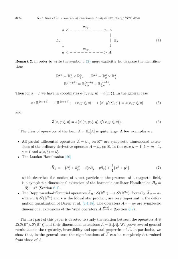
uniquely defined, for each Es, by the following commutative diagram
3774 N.C. Dias et al. / Journal of Functional Analysis 266 (2014) 3772–3796
aWeyl
< −−−−−−−−− > A
| |Es | | Es
↓ ↓a
Weyl< −−−−−−−−− > A.
(4)
Remark 2. In order to write the symbol a (2) more explicitly let us make the identifica-tions
R2n = R
nx × R
nξ , R
2k = Rky × R
kη,
R2(n+k) = R
(n+k)x,y × R
(n+k)ξ,η .
Then for s = I we have in coordinates a(x, y; ξ, η) = a(x, ξ). In the general case
s : R2(n+k) −→ R2(n+k); (x, y; ξ, η) −→
(x′, y′; ξ′, η′
)= s(x, y; ξ, η) (5)
and
a(x, y; ξ, η) = a(x′(x, y; ξ, η), ξ′(x, y; ξ, η)
). (6)
The class of operators of the form A = Es[A] is quite large. A few examples are:
• All partial differential operators A = ∂xion R
m are symplectic dimensional exten-sions of the ordinary derivative operator A = ∂x on R. In this case n = 1, k = m−1,s = I and a(x, ξ) = iξ.
• The Landau Hamiltonian [20]
HL = −(∂2x + ∂2
y
)+ i(x∂y − y∂x) + 1
4(x2 + y2) (7)
which describes the motion of a test particle in the presence of a magnetic field,is a symplectic dimensional extension of the harmonic oscillator Hamiltonian H0 =−∂2
x + x2 (Section 6.1).• The Bopp pseudo-differential operators AB : S(R2n) −→ S ′(R2n), formally AB = a
where a ∈ S ′(R2n) and is the Moyal star product, are very important in the defor-mation quantization of Bayen et al. [3,4,18]. The operators AB = a are symplecticdimensional extensions of the Weyl operators A
Weyl←→ a (Section 6.2).
The first part of this paper is devoted to study the relation between the operators A ∈L(S(Rn),S ′(Rn)) and their dimensional extensions A = Es[A]. We prove several generalresults about the regularity, invertibility and spectral properties of A. In particular, weshow that, in the general case, the eigenfunctions of A can be completely determinedfrom those of A.
N.C. Dias et al. / Journal of Functional Analysis 266 (2014) 3772–3796 3775
In the second part of the paper we define new classes of pseudo-differential operators,which are extensions of the Shubin classes of globally hypoelliptic operators. Using theresults of the first part, we prove a complete set of results about the spectral, invertibilityand hypoellipticity properties of the operators in the new classes. Finally, in Section 6 wepresent several examples of operators that belong to the new classes and have importantapplications in quantum mechanics and deformation quantization.
Notation. We will denote by S(Rm) the Schwartz space of rapidly decreasing functionson R
m; its dual S ′(Rm) is the space of tempered distributions. The space of linear andcontinuous operators of the form S(Rm) −→ S ′(Rm) is denoted by L(S(Rm),S ′(Rm)).The scalar product of two functions f, g ∈ L2(Rm) is denoted by (f |g) and the corre-sponding norm by ‖ · ‖. The distributional bracket is 〈 , 〉. The Euclidean product of twovectors x, y in R
m is written x·y and the norm of x ∈ Rm is |x|. The Weyl correspondence
is denoted by AWeyl←→ a or a
Weyl←→ A. The Weyl operators are also written A = Opw(a).The symplectic form on R
2n is defined by σn(z, z′) = Jz · z′ where J =(
0 I−I 0
). For
z = (x, ξ) and z′ = (x′, ξ′) we have explicitly σn(z, z′) = ξ · x′ − ξ′ · x. The extension tohigher dimensions is obviously σn+k = σn ⊕ σk, that is
σn+k
(z′, u′; z′′, u′′) = σn
(z′, z′′
)+ σk
(u′, u′′)
for (z′, u′), (z′′, u′′) ∈ R2n × R
2k.
2. Symplectic covariance of Weyl calculus: Review
For details and proofs we refer to Folland [13], de Gosson [15,17], or Wong [23].
2.1. Standard Weyl calculus
In view of Schwartz kernel theorem all operators A ∈ L(S(Rn),S ′(Rn)) admit therepresentation
Aψ(x) =⟨KA(x, ·), ψ(·)
⟩(8)
where KA ∈ S ′(Rn × Rn) and 〈 , 〉 is the distributional bracket. The Weyl symbol of A
is then
a(x, ξx) =∫Rn
e−iξx·yKA
(x + 1
2y, x− 12y
)dy (9)
with inverse
KA(x, y) =(
12π
)n ∫eiξ·(x−y)a
(x + y
2 , ξ
)dξ. (10)
Rn
3776 N.C. Dias et al. / Journal of Functional Analysis 266 (2014) 3772–3796
These integrals are well defined for a ∈ S(R2n) ⇐⇒ KA ∈ S(R2n), and should otherwisebe interpreted as generalized Fourier (or inverse Fourier) transforms (i.e. in the sense ofdistributions).
Substituting (10) in (8) and writing the distributional bracket as an integral we obtainthe standard formula for Weyl pseudo-differential operators
Aψ(x) = 1(2π)n
∫R2n
ei(x−y)·ξa
(12(x + y), ξ
)ψ(y) dy dξ. (11)
2.2. The metaplectic group
The symplectic group Sp(2n,R) of R2n ≡ R
n × Rn consists of all linear automor-
phisms s of R2n such that σn(s(z), s(z′)) = σn(z, z′) for all z, z′ ∈ R
2n. The groupSp(2n,R) is a connected classical Lie group; it has covering groups of all orders. Itsdouble cover admits a faithful (but not irreducible) representation by a group of unitaryoperators on L2(Rn), the metaplectic group Mp(2n,R). Thus, to every s ∈ Sp(2n,R)one can associate two unitary operators S and −S ∈ Mp(2n,R). One shows (Leray [21],de Gosson [14,15]) that every element of Mp(2n,R) is the product of exactly two Fourierintegral operators of the type
SW,mf(x) =(
12πi
)n/2
Δm(W )∫Rn
eiW (x,x′)f(x′) dx′ (12)
for f ∈ S(Rn) where
W(x, x′) = 1
2Px · x− Lx · x′ + 12Qx′ · x′
is a quadratic form with P = PT , Q = QT and detL �= 0, and
Δm(W ) = im√
|detL| (13)
where m is an integer (called the Maslov index) corresponding to a choice of arg detL.The operator SW,m belongs itself to Mp(2n,R) and corresponds to the element s ∈Sp(2n,R) characterized by the condition
(x, ξ) = s(x′, ξ′
)⇐⇒
{ξ = ∂xW
(x, x′),
ξ′ = −∂x′W(x, x′). (14)
It easily follows from the form of the generators (12) of Mp(2n,R) that metaplecticoperators are continuous mappings S(Rn) −→ S(Rn) which extend by duality to con-tinuous mappings S ′(Rn) −→ S ′(Rn). The inverse of the operator SW,m is given byS−1W,m = S∗
W,m = SW∗,m∗ where W ∗(x, x′) = −W (x′, x) and m∗ = n−m.
N.C. Dias et al. / Journal of Functional Analysis 266 (2014) 3772–3796 3777
2.3. Symplectic covariance
The following important property is characteristic of Weyl pseudo-differential calcu-lus:
Proposition 3. Let a ∈ S ′(R2n) and let A = Opw(a) be the corresponding Weyl pseudo-differential operator. Let s ∈ Sp(2n,R). We have
Opw(a ◦ s) = S−1 Opw(a)S (15)
where S is anyone of the elements of Mp(2n,R) corresponding to s.
This property has the following essential consequence for the symplectic dimensionalextensions. We will denote by S the elements of Mp(2(n+k),R) because these operatorsact on the “extended” space L2(Rn+k).
Proposition 4. Let s ∈ Sp(2(n+k),R) and a ∈ S ′(R2n). Let AI = EI [A] and As = Es[A]be the corresponding symplectic dimensional extensions of A = Opw(a). We have
As = S−1AI S (16)
where S ∈ Mp(2(n + k),R) is any of the two metaplectic operators that projects onto s.
Proof. In view of the definition of the dimensional extensions AI = EI [A] and As = Es[A]formula (16) is equivalent to
Opw[(a⊗ 12k) ◦ s
]= S−1 Opw
((a⊗ 12k)
)S (17)
and the latter is a straightforward consequence of Proposition 3. �From this property it is easy to deduce some continuity properties for the operators As
knowing those of AI . Suppose for instance that AI is bounded on L2(Rn+k) then so is As
since the metaplectic operators S ∈ Mp(2(n+k),R) are bounded on L2(Rn+k). It actuallysuffices in this case to assume that the operator A is bounded on L2(Rn) as will followfrom the intertwining results of the next section.
3. Properties of the dimensional extensions
3.1. A redefinition of A
We begin by making a few general observations. Assume that a ∈ S(R2n), A Weyl←→ a
and let A = EI [A]. Then, for Ψ ∈ S(Rn+k) we have from (11)
3778 N.C. Dias et al. / Journal of Functional Analysis 266 (2014) 3772–3796
AΨ(x, y) =(
12π
)n+k ∫R2(n+k)
ei[(x−x′)ξ+(y−y′)η]a
(12(x + x′), ξ)Ψ(x′, y′
)dx′ dy′ dξ dη
(18)
where the integral in η is viewed as the inverse Fourier transform of 1; we thus have
AΨ(x, y) =(
12π
)n ∫R2n
ei(x−x′)ξa
(12(x + x′), ξ)Ψ(x′, y
)dx′ dξ (19)
which we can write in compact form as
AΨ(·, y) = Aψy with ψy = Ψ(·, y). (20)
In particular, if ψ ∈ S(Rn) and φ ∈ S(Rk) then
A(ψ ⊗ φ) = (Aψ) ⊗ φ. (21)
These results can be extended to the more general case a ∈ S ′(R2n). In view offormula (8) we have
AΨ(z) =⟨KA(z, ·), Ψ(·)
⟩(22)
where z = (x, y) and KA ∈ S ′(Rn+k × Rn+k) is given by
KA
(x, y;x′, y′
)=
(12π
)n+k ∫Rn+k
eiξ·(x−x′)+iη(y−y′)a
(x + x′
2 , ξ
)dξ dη
= KA
(x;x′)δ(y − y′
)(23)
where the Fourier transform is interpreted in the sense of distributions and δ is the Diracmeasure. It follows from (23) that
AΨ(x, y) =⟨KA(x, ·), Ψ(·, y)
⟩=
⟨KA(x, ·), ψy(·)
⟩= Aψy(x) (24)
where, once again, ψy = Ψ(·, y). In particular, if Ψ = ψ ⊗ φ with ψ ∈ S(Rn) andφ ∈ S(Rk), we have again
A(ψ ⊗ φ) = (Aψ) ⊗ φ. (25)
This intertwining relation will be extended to the general case A = Es[A] in the nextsection.
N.C. Dias et al. / Journal of Functional Analysis 266 (2014) 3772–3796 3779
Another interesting formulation of A = EI [A], also valid in the case a ∈ S ′(R2n), isas follows. For Ψ,Φ ∈ S(Rn+k) the cross-Wigner transform is defined by [13,15,17]
W (Ψ,Φ)(x, y; ξ, η) =(
12π
)n+k ∫Rn×Rk
e−i(ξ·x′+η·y′)
× Ψ
((x, y) + 1
2(x′, y′
))Φ
((x, y) − 1
2(x′, y′
))dx′ dy′ (26)
and formula (18) is equivalent to
(AΨ |Φ)L2(Rn+k) =∫
R2(n+k)
a(x, ξ)W (Ψ,Φ)(x, y; ξ, η) dx dy dξ dη. (27)
Note that since W (Ψ,Φ) ∈ S(R2(n+k)) the integral above makes sense not only whena ∈ S(R2n), but also when a is measurable and does not increase too fast at infinity. Infact, viewing the integral as a distributional bracket, we can rewrite (27) as
〈AΨ, Φ〉 =⟨a,W (Ψ,Φ)
⟩(28)
which makes sense for every a = EI [a] ∈ S ′(R2(n+k)). More generally, we can redefinethe operator As = S−1AS = Es[A] by the formula
〈AsΨ, Φ〉 =⟨a ◦ s,W (Ψ,Φ)
⟩(29)
or, equivalently, by
〈AsΨ, Φ〉 =⟨a,W (SΨ, SΦ)
⟩. (30)
3.2. Composition, invertibility and adjoints
We will need the following result:
Lemma 5. If A is a continuous operator S(Rn) −→ S(Rn), then A = Es[A] is a contin-uous operator S(Rn+k) −→ S(Rn+k).
Proof. We first remark that it is sufficient to prove this result for s = I. This follows fromthe conjugation formula (16) in Proposition 4: if A : S(Rn+k) −→ S(Rn+k) then S−1AS :S(Rn+k) −→ S(Rn+k) since metaplectic operators preserve the Schwartz classes; thecontinuity statement follows likewise since metaplectic operators are unitary. Assumethat A is a continuous operator S(Rn) −→ S(Rn), and let A = EI [A] and Ψ ∈ S(Rn+k).Then, in view of formula (20), A is also continuous and AΨ ∈ S(Rn+k). �
3780 N.C. Dias et al. / Journal of Functional Analysis 266 (2014) 3772–3796
Recall that if AWeyl←→ a then the formal adjoint of A corresponds to the complex
conjugate of a, that is we have A∗ Weyl←→ a. In particular A is (formally) self-adjoint ifand only if its Weyl symbol is real. This property carries over to the case of symplecticdimensionally extended operators:
Proposition 6. We have
Es[A]∗ = Es
[A∗]. (31)
Hence, in particular, A = Es[A] is (formally) self-adjoint if and only if A is.
Proof. This property immediately follows from the definitions since we have Es[A] Weyl←→(a⊗ 12k) ◦ s and noting that the complex conjugate of (a⊗ 12k) ◦ s is (a⊗ 12k) ◦ s. �
The proof of the following composition property is slightly more technical; it showsthat the extension mapping Es preserves products of operators:
Proposition 7. Let A Weyl←→ a and BWeyl←→ b and assume that B : S(Rn) −→ S(Rn). In this
case A and B can be composed. Then A = Es[A] and B = Es[B] can also be composedand we have
Es[AB] = Es[A]Es[B]. (32)
Proof. That AB is well-defined follows from Lemma 5. Recall that the Weyl symbol ofthe product C = AB is given by the formula
c(z) =(
14π
)2n ∫R4n
ei2σn(z′,z′′)a
(z + 1
2z′)b
(z − 1
2z′′)dz′ dz′′ (33)
(see for instance [17, p. 148]). Let us first assume that s is the identity; then
a
(z + 1
2z′, u + 1
2u′)
= a
(z + 1
2z′),
b
(z − 1
2z′, u− 1
2u′)
= b
(z − 1
2z′)
and the Weyl symbol c of C = AB is thus given by
c(z, u) =(
14π
)2(n+k) ∫R4(n+k)
ei2σn+k(z′,u′;z′′,u′′)a
(z + 1
2z′)b
(z − 1
2z′′)dz′ dz′′ du′ du′′
=(
14π
)2(n+k) ∫e
i2σk(u′,u′′) du′ du′′
R4k
N.C. Dias et al. / Journal of Functional Analysis 266 (2014) 3772–3796 3781
×∫
R4n
ei2σn(z′,z′′)a
(z + 1
2z′)b
(z − 1
2z′′
)dz′ dz′′
=(
14π
)2n ∫R4n
ei2σn(z′,z′′)a
(z + 1
2z′)b
(z − 1
2z′′)dz′ dz′′
where we have used the relation σn+k = σn ⊕ σk and the Fourier inversion formula tocompute the integral in u′, u′′; thus c(z, u) = c(z) which proves our claim in the cases = I. The general case follows from formula (16) of Proposition 4. �
The next result is a corollary of the previous proposition.
Corollary 8. Let A−1 : S(Rn) −→ S(Rn) be the inverse of A : S(Rn) −→ S(Rn), i.e.AA−1 = A−1A = In where In is the identity operator in S(Rn). Then Es[A−1] is theinverse of Es[A], that is
Es
[A−1] =
(Es[A]
)−1. (34)
Proof. We first notice that Es[In] = In+k, which follows directly from (16) and (20).Then from (32)
Es[A]Es
[A−1] = Es
[AA−1] = Es[In] = In+k (35)
and likewise Es[A−1]Es[A] = In+k. Hence
Es
[A−1] =
(Es[A]
)−1. �
We notice for future reference that the composition and invertibility results extendby duality to S ′(Rn+k).
Remark 9. If A : S(Rn) −→ S(Rn) is linear and continuous then it extends by dualityto a continuous map that we shall denote by
A′ : S ′(R
n)−→ S ′(
Rn). (36)
We have, of course, A′|S(Rn) = A.In this case, A = Es[A] is also a linear and continuous map S(Rn+k) −→ S(Rn+k)
(Lemma 5) and so it also extends to a continuous map
A′ : S ′(R
n+k)−→ S ′(
Rn+k
).
Since both A′ and A′ are uniquely defined, we may extend the action of E to the operatorsA′ : S ′(Rn) −→ S ′(Rn) by setting
Es
[A′] := A′. (37)
3782 N.C. Dias et al. / Journal of Functional Analysis 266 (2014) 3772–3796
Let B be also a continuous map S(Rn) −→ S(Rn). It then follows trivially from thedefinition (37) that
Es
[A′B′] = Es
[A′]
Es
[B′] (38)
since A′B′ = (AB)′; and that
Es
[A′ −1] =
(Es
[A′])−1 (39)
since A′ −1 = (A−1)′.We conclude that the three maps ′, Es and −1 commute with each other in the space
of linear, continuous and invertible operators S(Rn) −→ S(Rn).
3.3. Intertwiners
For χ ∈ S(Rk) and S ∈ Mp(2(n + k),R) let us define the operator TS,χ : S(Rn) −→S(Rn+k) by the formula
TS,χψ = S−1(ψ ⊗ χ). (40)
These operators TS,χ have the following analytical properties:
Proposition 10. The operator TS,χ extends to a continuous map S ′(Rn) −→ S ′(Rn+k)and, if ‖χ‖ = 1, to a partial isometry L2(Rn) −→ L2(Rn+k).
The adjoint T ∗S,χ
: L2(Rn+k) −→ L2(Rn) is given by the formula
T ∗S,χ
Φ(x) =∫Rk
χ(y)SΦ(x, y) dy (41)
and also extends to the continuous operator S ′(Rn+k) −→ S ′(Rn) defined by⟨T ∗S,χ
Φ,ψ⟩
= 〈SΦ, χ⊗ ψ〉, ∀ψ ∈ S(R
n). (42)
Proof. Let ψ ∈ S ′(Rn); then ψ ⊗ χ ∈ S ′(Rn+k) and hence S−1(ψ ⊗ χ) ∈ S ′(Rn+k). Theformula TS,χψ = S−1(ψ ⊗ χ) defines the desired extension. Assume now ‖χ‖ = 1 andψ ∈ L2(Rn); dropping for notational simplicity the references to the spaces in scalarproducts and norms we have
‖TS,χψ‖2 =
∥∥S−1(ψ ⊗ χ)∥∥2 = ‖ψ ⊗ χ‖2
since S is unitary. Now ‖ψ⊗χ‖2 = ‖ψ‖2‖χ‖2 hence TS,χ is a partial isometry. Its adjointis defined by (T ∗˜ Φ|ψ) = (Φ|T ˜ ψ). Formula (41) follows since we have
S,χ S,χ
N.C. Dias et al. / Journal of Functional Analysis 266 (2014) 3772–3796 3783
(Φ|TS,χψ) =(Φ|S−1(ψ ⊗ χ)
)= (SΦ|ψ ⊗ χ)
=∫Rn
ψ(x)[ ∫Rk
χ(y)SΦ(x, y) dy]dx.
Finally, using distributional brackets and the definition of the adjoint, the previous equa-tion can be re-written as
⟨T ∗S,χ
Φ,ψ⟩
= 〈SΦ, χ⊗ ψ〉, ∀ψ ∈ S(R
n)
which defines the distribution T ∗S,χ
Φ ∈ S ′(Rn) for every Φ ∈ S ′(Rn+k). �The following intertwining relations are essential for studying the spectral properties
of the symplectic dimensional extensions:
Proposition 11. Let s ∈ Sp(2(n + k),R) and S be one of the two metaplectic operatorsthat projects onto s. Then
AsTS,χ = TS,χA, T ∗S,χ
As = AT ∗S,χ
(43)
for every A = Opw(a), a ∈ S ′(R2n) and As = Es[A].
Proof. Let us first prove that AsTS,χ = TS,χA for the case S = I. Let us set Tχ = TI,χ
and let ψ ∈ S(Rn). In view of formula (24) we have
AI(Tχψ)(x, y) = A(Tχψ)y(x)
= Aψ(x)χ(y)
= Tχ(Aψ)(x, y).
The general case follows using formula (16) since
AsTS,χ = S−1AI S(S−1Tχ
)= S−1AITχ
= S−1TχA
= TS,χA.
The second formula (43) is deduced from the first: since A∗sTS,χ = TS,χA
∗ (because ofthe equality (31)), we have (A∗
sTS,χ)∗ = (TS,χA∗)∗ that is T ∗
S,χAs = AT ∗
S,χ. �
3784 N.C. Dias et al. / Journal of Functional Analysis 266 (2014) 3772–3796
4. Spectral results
4.1. Orthonormal bases and the partial isometries TS,χ
In view of Proposition 10 the intertwining operators TS,χ are partial isometries ofL2(Rn) into L2(Rn+k). Hence the range HS,χ of TS,χ is a closed subspace of L2(Rn+k).The following result shows how the operators TS,χ generate orthonormal bases ofL2(Rn+k).
Proposition 12. Let (φj)j be an orthonormal basis of L2(Rn) and (χl)l an orthonormalbasis of L2(Rk). Then (TS,χl
φj)j,l is an orthonormal basis of L2(Rn+k) and L2(Rn+k) =⊕l HS,χl
.
Proof. Let us set Φj,l = TS,χlφj . We have
(Φj,l|Φj′,l′) =(S−1(φj ⊗ χl)|S−1(φj′ ⊗ χl′)
)= (φj ⊗ χl|φj′ ⊗ χl′)
= (φj |φj′)(χl|χl′)
hence the vectors Φj,l form an orthonormal system in L2(Rn+k). Let us prove that thissystem is complete in L2(Rn+k); it suffices for that to show that if Ψ ∈ L2(Rn+k) is suchthat (Ψ |Φj,l) = 0 for all indices j, l then Ψ = 0. Now,
(Ψ |Φj,l) =(Ψ |S−1(φj ⊗ χl)
)= (SΨ |φj ⊗ χl)
and (Ψ |Φj,l) = 0 for all j, l implies SΨ = 0 because the tensor product of the twoorthonormal bases is an orthonormal basis of L2(Rn+k); it follows that Ψ = 0 as claimed.Moreover, for each l the set (Φj,l)j is an orthonormal basis of HS,χl
. Since for l �= l′ wehave HS,χl
∩HS,χl′= {0} it follows that L2(Rn+k) =
⊕l HS,χl
. �The observant Reader will have noticed that in the first part of the proof we established
the equality (TS,χφ|TS,χ′φ
′)L2(Rn+k) =
(φ|φ′)
L2(Rn)
(χ|χ′)
L2(Rk) (44)
which is valid for all pairs of functions (φ, φ′) in L2(Rn) and (χ, χ′) in L2(Rk).
4.2. Spectral result
Let us prove the main result of this section:
Proposition 13. Let s ∈ Sp(2(n+k),R), let A : S(Rn) �−→ S ′(Rn) be a linear continuousoperator and let As = Es[A]. Let S be one of the metaplectic operators associated with s.Then:
N.C. Dias et al. / Journal of Functional Analysis 266 (2014) 3772–3796 3785
(i) The eigenvalues of A and As are the same.(ii) If ψ is an eigenfunction of A corresponding to the eigenvalue λ then Ψ = TS,χψ is
an eigenfunction of As corresponding to λ, for every χ ∈ S(Rk)\{0}, and we haveΨ ∈ S(Rn+k).
(iii) Conversely, if Ψ is an eigenfunction of As and ψ = T ∗S,χ
Ψ is different from zerothen ψ is an eigenfunction of A and corresponds to the same eigenvalue.
(iv) If (ψj)j is an orthonormal basis of eigenfunctions of A and (χl ∈ S(Rk))l is anorthonormal basis of L2(Rk) then (TS,χl
ψj)j,l is a complete set of eigenfunctionsof As and forms an orthonormal basis of L2(Rn+k).
Proof. That every eigenvalue of A also is an eigenvalue of As is clear: if Aψ = λψ forsome ψ �= 0 then
As(TS,χψ) = TS,χAψ = λ(TS,χψ)
and TS,χψ �= 0 because TS,χ is injective; this shows at the same time that Ψ = TS,χψ
is an eigenfunction of As. Since TS,χ : S(Rn) −→ S(Rn+k) it is clear that Ψ ∈ S(Rn+k)which concludes the proof of (ii).
Assume conversely that AsΨ = λΨ and Ψ �= 0. For every χ we have, using the secondintertwining relation (43),
AT ∗S,χ
Ψ = T ∗S,χ
AsΨ = λT ∗S,χ
Ψ
hence λ is an eigenvalue of A and T ∗S,χ
Ψ will be an eigenfunction of A if it is differentfrom zero. This proves (iii).
To conclude the proof of (i) we still have to show that if Ψ is an eigenfunction of As
then T ∗S,χ
Ψ �= 0 for some χ ∈ S(Rk). We note that TS,χT∗S,χ
= PS,χ is the orthogonalprojection onto the range HS,χ of TS,χ. Assume that T ∗
S,χΨ = 0 for all χ ∈ S(Rk); then
PS,χΨ = 0 for every χ ∈ S(Rk), and hence Ψ = 0 in view of Proposition 12; but this isnot possible since Ψ is an eigenfunction.
Finally, the statement (iv) follows from (ii) and Proposition 12. �4.3. Generalized spectral theorem
If A is a continuous linear operator S(Rn) −→ S(Rn) then it can be extended toa continuous operator S ′(Rn) −→ S ′(Rn). In view of Lemma 5, As = Es[A] is also acontinuous operator S(Rn+k) −→ S(Rn+k) and thus can also be extended to a continuousoperator S ′(Rn+k) −→ S ′(Rn+k). In this case Proposition 13 can be extended to ageneralized spectral result. Let (ψ, λ) ∈ S ′(Rn) × C. We will say that ψ is a generalizedeigenvector of A, corresponding to the generalized eigenvalue λ if ψ �= 0 and⟨
ψ,A∗φ⟩
= λ〈ψ, φ〉 for all φ ∈ S(R
n).
3786 N.C. Dias et al. / Journal of Functional Analysis 266 (2014) 3772–3796
We will write this equality formally as (ψ|A∗φ) = λ(ψ|φ) since both sides coincide withthe usual scalar products when ψ is a square integrable function.
Proposition 14. Assume that A is a continuous linear operator of the form A : S(Rn) −→S(Rn) and let As = Es[A]. Then:
(i) The generalized eigenvalues of the operators A and As are the same.(ii) Let ψ be a generalized eigenvector of A. Then, for every χ ∈ S(Rk)\{0} the vector
Ψ = TS,χψ is a generalized eigenvector of As and corresponds to the same general-ized eigenvalue.
(iii) Conversely, if Ψ is a generalized eigenvector of As and ψ = T ∗S,χ
Ψ �= 0 then ψ is ageneralized eigenvector of A corresponding to the same generalized eigenvalue.
Proof. It is similar, mutatis mutandis, to the proof of Theorem 445, Chapter 19, in [17](also see [16]). For instance, to prove (ii) one notes that if (ψ|A∗φ) = λ(ψ|φ) for everyφ ∈ S(Rn) then also (TS,χψ|A∗
sΦ) = λ(TS,χψ|Φ) for every Φ ∈ S(Rn+k). In fact, usingthe intertwining property (43),(
TS,χψ|A∗sΦ
)=
(ψ|T ∗
S,χA∗
sΦ)
=(ψ|(AsTS,χ)∗Φ
)=
(ψ|(TS,χA)∗Φ
)=
(ψ|A∗T ∗
S,χΦ)
= λ(ψ|T ∗
S,χΦ)
hence the claim. �5. A new class of pseudo-differential operators
In this section we define a new class of pseudo-differential operators which is an ex-tension of the well-known Shubin class HGm1,m0
ρ (R2n) of globally hypoelliptic operators.Moreover, we prove several general results about the spectral, invertibility and hypoel-lipticity properties of the operators in the new class.
5.1. The Shubin classes of global hypoelliptic operators
A linear operator A : S ′(Rn) −→ S ′(Rn) is “globally hypoelliptic” if it satisfies
ψ ∈ S ′(R
n)
and Aψ ∈ S(R
n)
=⇒ ψ ∈ S(R
n). (45)
This notion is different with respect to the ordinary C∞ hypoellipticity (which is alocal property) because it incorporates the decay at infinity of the involved functions ordistributions.
N.C. Dias et al. / Journal of Functional Analysis 266 (2014) 3772–3796 3787
The Shubin class of globally hypoelliptic operators HGm1,m0ρ (R2n) is a subclass of the
Shubin class Gm1ρ (R2n). It is defined (Shubin [22], de Gosson [17]) as follows:
Definition 15. Let m0, m1, and ρ be real numbers such that m0 � m1 and 0 < ρ � 1.The symbol class HΓm1,m0
ρ (R2n) consists of all functions a ∈ C∞(R2n) such that for |z|sufficiently large the following estimates hold:
C0|z|m0 �∣∣a(z)∣∣ � C1|z|m1 (46)
for some C0, C1 > 0 and, for every α ∈ N2n there exists Cα � 0 such that∣∣∂α
z a(z)∣∣ � Cα
∣∣a(z)∣∣|z|−ρ|α|. (47)
The Shubin class HGm1,m0ρ (R2n) consists of all operators A : S(Rn) −→ S ′(Rn) with
Weyl symbols a ∈ HΓm1,m0ρ (R2n).
The main appeal of the classes HGm1,m0ρ (R2n) is the set of general properties which is
satisfied by their operators. Moreover, they contain many operators which are importantin mathematical physics (a trivial example is the harmonic oscillator Hamiltonian). Letus then state the main properties of the operators in HGm1,m0
ρ (R2n) (for proofs see [22,Chapter IV]).
Since HΓm1,m0ρ (R2n) ⊂ Γm1
ρ (R2n), every operator A ∈ HGm1,m0ρ (R2n) is a continuous
operator S(Rn) −→ S(Rn) which extends by duality to a continuous operator S ′(Rn) −→S ′(Rn). Moreover,
Proposition 16 (Shubin). Let A ∈ HGm1,m0ρ (R2n) with m0 > 0. If A is formally self-
adjoint, that is if (Aψ|φ) = (ψ|Aφ) for all test functions ψ, φ ∈ S(Rn), then A isessentially self-adjoint and has discrete spectrum in L2(Rn). Moreover there exists anorthonormal basis of eigenfunctions φj ∈ S(Rn) (j = 1, 2, . . .) with eigenvalues λj ∈ R
such that limj−→∞ |λj | = ∞.
In addition, every A ∈ HGm1,m0ρ (R2n) is globally hypoelliptic and, if KerA =
KerA∗ = {0}, it is also invertible with inverse A−1 ∈ HG−m0,−m1ρ (R2n).
5.2. The extended Shubin classes HGm1,m0
ρ (R2n)
We now define a new class of pseudo-differential operators:
Definition 17. The symbol class HΓm1,m0
ρ (R2n) consists of all functions a ∈ C∞(R2n) forwhich there is a ∈ HΓm1,m0
ρ (R2(n−k)) (for some k ∈ {0, 1, . . . , n− 1}) and a symplecticextension map Es : S ′(R2(n−k)) −→ S ′(R2n) such that a = Es[a]. The set of pseudo-differential operators with Weyl symbols a ∈ HΓ
m1,m0
ρ (R2n) is called an “extendedShubin class” and denoted by HG
m1,m0
ρ (R2n).
3788 N.C. Dias et al. / Journal of Functional Analysis 266 (2014) 3772–3796
We notice that, by construction, the symbols in the classes HΓm1,m0
ρ (R2n) satisfy theproperty
a ∈ HΓm1,m0
ρ
(R
2n) ⇐⇒ a ◦ s ∈ HΓm1,m0
ρ
(R
2n), ∀s ∈ Sp(2n,R).
Apart from the trivial case k = 0 or the case where a(z) is a polynomial, the symbol Es[a]does not belong any more to the Shubin classes. Hence the Shubin results concerninghypoellipticity and spectral theory do not apply to the operators in the extended Shubinclasses of Definition 17.
In the next section we will present several examples of operators in the classesHG
m1,m0
ρ (R2n), which are important for applications in quantum mechanics and de-formation quantization. First, let us study the general properties of the operators inHG
m1,m0
ρ (R2n).
Lemma 18. Let A ∈ HGm1,m0
ρ (R2n) and let A ∈ HGm1,m0ρ (R2(n−k)) be the associated
operator such that A = Es[A]. Then Ker A = {0} iff KerA = {0}. (To be clear, bothoperators are considered as continuous maps of the form S(Rm) −→ S(Rm), wherem = n and m = n− k for A and A, respectively.)
Proof. Assume that KerA �= {0} and let ψ ∈ S(Rn−k)\{0} be such that Aψ = 0. LetΨ = TS,χψ = S−1ψ ⊗ χ, where S is (one of the two) metaplectic operators associatedwith s, and χ ∈ S(Rk)\{0}. Then Ψ �= 0 and in view of Proposition 11
AΨ = ATS,χψ = TS,χAψ = 0.
We conclude that Ker A �= {0}.Conversely, assume that Ker A �= {0} and let Ψ ∈ S(Rn)\{0} be such that AΨ = 0.
Once again, in view of Proposition 11 we have for ψ = T ∗S,χ
Ψ
Aψ = AT ∗S,χ
Ψ = T ∗S,χ
AΨ = 0.
It remains to prove that there is always some χ ∈ S(Rk) such that ψ = T ∗S,χ
Ψ �= 0. FromProposition 12 we know that (TS,χl
φj)jl is an orthogonal basis of L2(Rn) provided (φj)jand (χl)l are orthogonal bases of L2(Rn−k) and L2(Rk), respectively. In addition, wemay choose φj ∈ S(Rn−k) and χl ∈ S(Rk). It follows that there is always some l, j suchthat
(Ψ |TS,χlφj) =
(T ∗S,χl
Ψ |φj
)�= 0
and so ψ = T ∗S,χl
Ψ �= 0, which concludes the proof. �
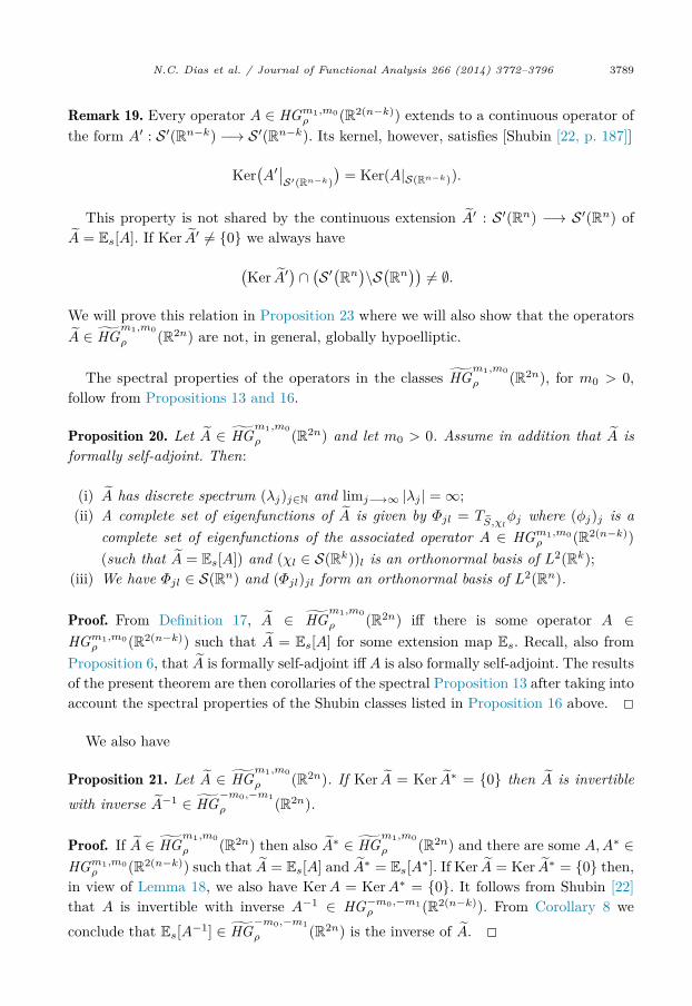
N.C. Dias et al. / Journal of Functional Analysis 266 (2014) 3772–3796 3789
Remark 19. Every operator A ∈ HGm1,m0ρ (R2(n−k)) extends to a continuous operator of
the form A′ : S ′(Rn−k) −→ S ′(Rn−k). Its kernel, however, satisfies [Shubin [22, p. 187]]
Ker(A′∣∣
S′(Rn−k)
)= Ker(A|S(Rn−k)).
This property is not shared by the continuous extension A′ : S ′(Rn) −→ S ′(Rn) ofA = Es[A]. If Ker A′ �= {0} we always have
(Ker A′) ∩ (
S ′(R
n)\S
(R
n))
�= ∅.
We will prove this relation in Proposition 23 where we will also show that the operatorsA ∈ HG
m1,m0
ρ (R2n) are not, in general, globally hypoelliptic.
The spectral properties of the operators in the classes HGm1,m0
ρ (R2n), for m0 > 0,follow from Propositions 13 and 16.
Proposition 20. Let A ∈ HGm1,m0
ρ (R2n) and let m0 > 0. Assume in addition that A isformally self-adjoint. Then:
(i) A has discrete spectrum (λj)j∈N and limj−→∞ |λj | = ∞;(ii) A complete set of eigenfunctions of A is given by Φjl = TS,χl
φj where (φj)j is acomplete set of eigenfunctions of the associated operator A ∈ HGm1,m0
ρ (R2(n−k))(such that A = Es[A]) and (χl ∈ S(Rk))l is an orthonormal basis of L2(Rk);
(iii) We have Φjl ∈ S(Rn) and (Φjl)jl form an orthonormal basis of L2(Rn).
Proof. From Definition 17, A ∈ HGm1,m0
ρ (R2n) iff there is some operator A ∈HGm1,m0
ρ (R2(n−k)) such that A = Es[A] for some extension map Es. Recall, also fromProposition 6, that A is formally self-adjoint iff A is also formally self-adjoint. The resultsof the present theorem are then corollaries of the spectral Proposition 13 after taking intoaccount the spectral properties of the Shubin classes listed in Proposition 16 above. �
We also have
Proposition 21. Let A ∈ HGm1,m0
ρ (R2n). If Ker A = Ker A∗ = {0} then A is invertiblewith inverse A−1 ∈ HG
−m0,−m1
ρ (R2n).
Proof. If A ∈ HGm1,m0
ρ (R2n) then also A∗ ∈ HGm1,m0
ρ (R2n) and there are some A,A∗ ∈HGm1,m0
ρ (R2(n−k)) such that A = Es[A] and A∗ = Es[A∗]. If Ker A = Ker A∗ = {0} then,in view of Lemma 18, we also have KerA = KerA∗ = {0}. It follows from Shubin [22]that A is invertible with inverse A−1 ∈ HG−m0,−m1
ρ (R2(n−k)). From Corollary 8 weconclude that Es[A−1] ∈ HG
−m0,−m1
ρ (R2n) is the inverse of A. �
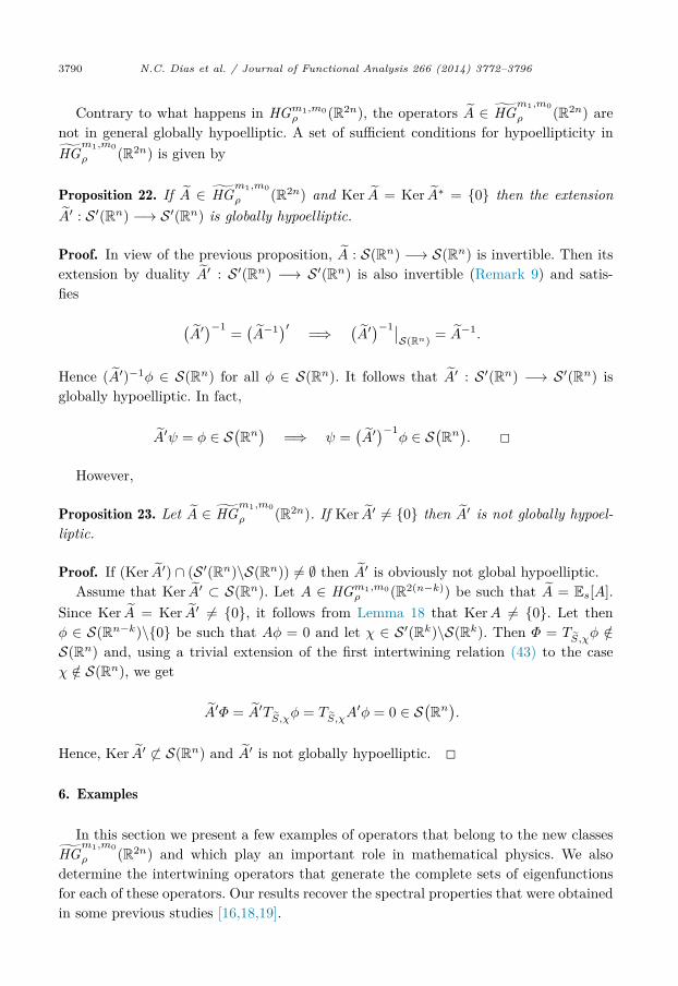
3790 N.C. Dias et al. / Journal of Functional Analysis 266 (2014) 3772–3796
Contrary to what happens in HGm1,m0ρ (R2n), the operators A ∈ HG
m1,m0
ρ (R2n) arenot in general globally hypoelliptic. A set of sufficient conditions for hypoellipticity inHG
m1,m0
ρ (R2n) is given by
Proposition 22. If A ∈ HGm1,m0
ρ (R2n) and Ker A = Ker A∗ = {0} then the extensionA′ : S ′(Rn) −→ S ′(Rn) is globally hypoelliptic.
Proof. In view of the previous proposition, A : S(Rn) −→ S(Rn) is invertible. Then itsextension by duality A′ : S ′(Rn) −→ S ′(Rn) is also invertible (Remark 9) and satis-fies
(A′)−1 =
(A−1)′ =⇒
(A′)−1∣∣
S(Rn) = A−1.
Hence (A′)−1φ ∈ S(Rn) for all φ ∈ S(Rn). It follows that A′ : S ′(Rn) −→ S ′(Rn) isglobally hypoelliptic. In fact,
A′ψ = φ ∈ S(R
n)
=⇒ ψ =(A′)−1
φ ∈ S(R
n). �
However,
Proposition 23. Let A ∈ HGm1,m0
ρ (R2n). If Ker A′ �= {0} then A′ is not globally hypoel-liptic.
Proof. If (Ker A′) ∩ (S ′(Rn)\S(Rn)) �= ∅ then A′ is obviously not global hypoelliptic.Assume that Ker A′ ⊂ S(Rn). Let A ∈ HGm1,m0
ρ (R2(n−k)) be such that A = Es[A].Since Ker A = Ker A′ �= {0}, it follows from Lemma 18 that KerA �= {0}. Let thenφ ∈ S(Rn−k)\{0} be such that Aφ = 0 and let χ ∈ S ′(Rk)\S(Rk). Then Φ = TS,χφ /∈S(Rn) and, using a trivial extension of the first intertwining relation (43) to the caseχ /∈ S(Rn), we get
A′Φ = A′TS,χφ = TS,χA′φ = 0 ∈ S
(R
n).
Hence, Ker A′ �⊂ S(Rn) and A′ is not globally hypoelliptic. �6. Examples
In this section we present a few examples of operators that belong to the new classesHG
m1,m0
ρ (R2n) and which play an important role in mathematical physics. We alsodetermine the intertwining operators that generate the complete sets of eigenfunctionsfor each of these operators. Our results recover the spectral properties that were obtainedin some previous studies [16,18,19].
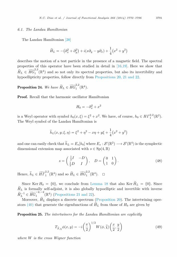
N.C. Dias et al. / Journal of Functional Analysis 266 (2014) 3772–3796 3791
6.1. The Landau Hamiltonian
The Landau Hamiltonian [20]
HL = −(∂2x + ∂2
y
)+ i(x∂y − y∂x) + 1
4(x2 + y2)
describes the motion of a test particle in the presence of a magnetic field. The spectralproperties of this operator have been studied in detail in [16,19]. Here we show thatHL ∈ HG
2,21 (R4) and so not only its spectral properties, but also its invertibility and
hypoellipticity properties, follow directly from Propositions 20, 21 and 22.
Proposition 24. We have HL ∈ HG2,21 (R4).
Proof. Recall that the harmonic oscillator Hamiltonian
H0 = −∂2x + x2
is a Weyl operator with symbol h0(x, ξ) = ξ2 + x2. We have, of course, h0 ∈ HΓ 2,21 (R2).
The Weyl symbol of the Landau Hamiltonian is
hL(x, y; ξ, η) = ξ2 + η2 − xη + yξ + 14(x2 + y2)
and one can easily check that hL = Es[h0] where Es : S ′(R2) −→ S ′(R4) is the symplecticdimensional extension map associated with s ∈ Sp(4,R)
s =( 1
2I −D12D I
), D =
(0 11 0
). (48)
Hence, hL ∈ HΓ2,21 (R4) and so HL ∈ HG
2,21 (R4). �
Since KerH0 = {0}, we conclude from Lemma 18 that also Ker HL = {0}. SinceHL is formally self-adjoint, it is also globally hypoelliptic and invertible with inverseH−1
L ∈ HG−2,−21 (R4) (Propositions 21 and 22).
Moreover, HL displays a discrete spectrum (Proposition 20). The intertwining oper-ators (40) that generate the eigenfunctions of HL from those of H0 are given by
Proposition 25. The intertwiners for the Landau Hamiltonian are explicitly
TS,χφ(x, y) = −i
(π
2
)1/2
W (φ, χ)(x
2 ,y
2
)(49)
where W is the cross Wigner function
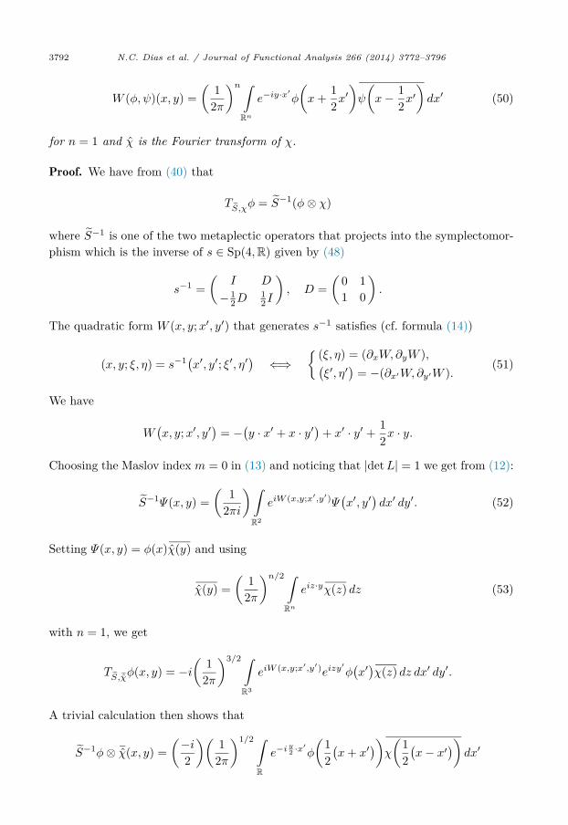
3792 N.C. Dias et al. / Journal of Functional Analysis 266 (2014) 3772–3796
W (φ, ψ)(x, y) =(
12π
)n ∫Rn
e−iy·x′φ
(x + 1
2x′)ψ
(x− 1
2x′)dx′ (50)
for n = 1 and χ is the Fourier transform of χ.
Proof. We have from (40) that
TS,χφ = S−1(φ⊗ χ)
where S−1 is one of the two metaplectic operators that projects into the symplectomor-phism which is the inverse of s ∈ Sp(4,R) given by (48)
s−1 =(
I D
−12D
12I
), D =
(0 11 0
).
The quadratic form W (x, y;x′, y′) that generates s−1 satisfies (cf. formula (14))
(x, y; ξ, η) = s−1(x′, y′; ξ′, η′)
⇐⇒{ (ξ, η) = (∂xW,∂yW ),(
ξ′, η′)
= −(∂x′W,∂y′W ).(51)
We have
W(x, y;x′, y′
)= −
(y · x′ + x · y′
)+ x′ · y′ + 1
2x · y.
Choosing the Maslov index m = 0 in (13) and noticing that |detL| = 1 we get from (12):
S−1Ψ(x, y) =(
12πi
)∫R2
eiW (x,y;x′,y′)Ψ(x′, y′
)dx′ dy′. (52)
Setting Ψ(x, y) = φ(x)χ(y) and using
χ(y) =(
12π
)n/2 ∫Rn
eiz·yχ(z) dz (53)
with n = 1, we get
TS,χφ(x, y) = −i
(12π
)3/2 ∫R3
eiW (x,y;x′,y′)eizy′φ(x′)χ(z) dz dx′ dy′.
A trivial calculation then shows that
S−1φ⊗ χ(x, y) =(−i
2
)(12π
)1/2 ∫e−i y
2 ·x′φ
(12(x + x′))χ(1
2(x− x′
))dx′
R
N.C. Dias et al. / Journal of Functional Analysis 266 (2014) 3772–3796 3793
and so
TS,χφ(x, y) = −i
(π
2
)1/2
W (φ, χ)(x
2 ,y
2
).
Taking into account that ϕ = χ =⇒ χ = ϕ we easily obtain (49). �This result coincides exactly with the formula for the intertwiners that was obtained
in [16,19].
6.2. Bopp pseudo-differential operators
Let a ∈ S ′(R2n) and consider the operator defined by
AB : S(R
2n) −→ S ′(R
2n); Ψ −→ ABΨ = a Ψ (54)
where is the Moyal star-product
a b(z) =(
14π
)2n ∫R2n×R2n
e−i2σn(v,u)a
(z + 1
2u)b
(z − 1
2v)du dv (55)
familiar from deformation quantization [3,4,11,12]. The operators AB = a are usuallycalled “Bopp pseudo-differential operators” [7] (or “Moyal–Weyl pseudo-differential op-erators” [10]) and are very important in deformation quantization where they were used,for instance, to obtain a precise formulation of the spectral problem [18].
Moreover, the map a −→ AB = a yields a phase space representation of quantummechanics [10], called the “Moyal representation”, that finds interesting applications insemiclassical dynamics [6], hybrid dynamics [5] and non-commutative quantum mechan-ics [1,2,8,9].
In this section we show that for every a ∈ HΓm1,m0ρ (R2n), the operator AB = a
belongs to HGm1,m0
ρ (R4n). Hence its spectral, invertibility and hypoellipticity propertiesare given by our Propositions 20, 21, 22 and 23.
We start by recalling that:
Lemma 26. Let a ∈ S ′(R2n). Then the operator formally AB = a is a Weyl operatorS(R2n) −→ S ′(R2n) with symbol
aB(x, y; ξ, η) = a
(x− 1
2η, y + 12ξ
). (56)
For a proof see [18]. We then have
Proposition 27. Let a ∈ HΓm1,m0ρ (R2n). Then AB ∈ HG
m1,m0
ρ (R4n).
3794 N.C. Dias et al. / Journal of Functional Analysis 266 (2014) 3772–3796
Proof. The Weyl symbol aB (56) is given by aB = Es[a] where Es : S ′(R2n) −→ S ′(R4n)is the symplectic dimensional extension map associated with the symplectomorphisms ∈ Sp(4n,R)
s =(
I −12D
D 12I
), D =
(0 I
I 0
). (57)
Hence, for a ∈ HΓm1,m0ρ (R2n) we have
aB ∈ HΓm1,m0
ρ (R4n) and so AB ∈ HGm1,m0
ρ (R4n). �Let us then determine the explicit form of the intertwining operators that generate
the eigenfunctions of AB = a from those of A = Opw(a).
Proposition 28. The intertwiners for the Bopp operators are given by
TS,χφ = (2π)n/2i−nW (φ, χ) (58)
where W is the cross-Wigner function (50).
Proof. The intertwining operators are given by TS,χφ = S−1φ ⊗ χ where S−1 is (oneof the two) metaplectic operators that project into the symplectomorphism s−1 ∈Sp(4n,R), inverse of (57).
s−1 =( 1
2I12D
−D I
), D =
(0 I
I 0
).
From (51) we find the quadratic form that generates s−1
W(x, y;x′, y′
)= −2
(y · x′ + x · y′
)+ x′ · y′ + 2x · y.
Choosing the Maslov index m = 0 in (13) and taking into account that |detL| = 22n weget from (12)
S−1Ψ(x, y) =(
1πi
)n ∫R2n
eiW (x,y;x′,y′)Ψ(x′, y′
)dx′ dy′. (59)
Setting Ψ = φ⊗ χ and using (53) we get
TS,χφ(x, y) =(
12π
)n/2( 1iπ
)n ∫R3n
eiW (x,y;x′,y′)eiz·y′φ(x′)χ(z) dz dx′ dy′
=(
2π
)n/2
i−n
∫e−iy·(2x′−2x)φ
(x′)χ(2x− x′
)dx′.
Rn
N.C. Dias et al. / Journal of Functional Analysis 266 (2014) 3772–3796 3795
Making the change of variables x′′ = 2x′ − 2x and taking into account that ϕ = χ =⇒χ = ϕ we easily obtain (58). �Acknowledgments
The authors would like to thank the anonymous referee for making an importantcorrection in Section 5.
Nuno Costa Dias and João Nuno Prata have been supported by the research grantPTDC/MAT/099880/2008 of the Portuguese Science Foundation (FCT). Maurice deGosson has been supported by a research grant from the Austrian Research AgencyFWF (Projektnummer P23902-N13).
References
[1] C. Bastos, O. Bertolami, N.C. Dias, J.N. Prata, Weyl–Wigner formulation of noncommutativequantum mechanics, J. Math. Phys. 49 (2008) 072101, 24 pp.
[2] C. Bastos, N.C. Dias, J.N. Prata, Wigner measures in noncommutative quantum mechanics, Comm.Math. Phys. 299 (3) (2010) 709–740.
[3] F. Bayen, M. Flato, C. Fronsdal, A. Lichnerowicz, D. Sternheimer, Deformation theory and quan-tization. I. Deformation of symplectic structures, Ann. Physics 110 (1978) 111–151.
[4] F. Bayen, M. Flato, C. Fronsdal, A. Lichnerowicz, D. Sternheimer, Deformation theory and quan-tization. II. Physical applications, Ann. Physics 111 (1978) 6–110.
[5] D.I. Bondar, R. Cabrera, R.R. Lompay, M.Y. Ivanov, H.A. Rabitz, Operational dynamical modelingtranscending quantum and classical mechanics, Phys. Rev. Lett. 109 (2012) 190403.
[6] D.I. Bondar, R. Cabrera, H.A. Rabitz, Wigner function’s negativity demystified, arXiv:1202.3628,2012.
[7] F. Bopp, La mécanique quantique est-elle une mécanique statistique particulière?, Ann. Inst. H.Poincaré 15 (1956) 81–112.
[8] N.C. Dias, M. de Gosson, F. Luef, J.N. Prata, A deformation quantization theory for non-commutative quantum mechanics, J. Math. Phys. 51 (2010) 072101, 12 pp.
[9] N.C. Dias, M. de Gosson, F. Luef, J.N. Prata, A pseudo-differential calculus on non-standard sym-plectic space; spectral and regularity results in modulation spaces, J. Math. Pures Appl. 96 (2011)423–445.
[10] N.C. Dias, M. de Gosson, F. Luef, J.N. Prata, Quantum mechanics in phase space: the Schrödingerand the Moyal representations, J. Pseudo-Differ. Oper. Appl. 3 (4) (2012) 367–398.
[11] N.C. Dias, J.N. Prata, Formal solutions of stargenvalue equations, Ann. Phys. (N. Y.) 311 (2004)120–151.
[12] N.C. Dias, J.N. Prata, Admissible states in quantum phase space, Ann. Phys. (N. Y.) 313 (2004)110–146.
[13] G.B. Folland, Harmonic Analysis in Phase Space, Ann. of Math. Stud., Princeton University Press,Princeton, NJ, 1989.
[14] M. de Gosson, Maslov Classes, Metaplectic Representation and Lagrangian Quantization, Res. NotesMath., vol. 95, Wiley–VCH, Berlin, 1997.
[15] M. de Gosson, Symplectic Geometry and Quantum Mechanics, Oper. Theory Adv. Appl. (Adv.Partial Differ. Equ.), vol. 166, Birkhäuser, Basel, 2006.
[16] M. de Gosson, Spectral properties of a class of generalized Landau operators, Comm. Partial Dif-ferential Equations 33 (11) (2008) 2096–2104.
[17] M. de Gosson, Symplectic Methods in Harmonic Analysis and in Mathematical Physics, Birkhäuser,Springer, Basel, 2011.
[18] M. de Gosson, F. Luef, A new approach to the �-genvalue equation, Lett. Math. Phys. 85 (2008)173–183.
[19] M. de Gosson, F. Luef, Spectral and regularity properties of a pseudo-differential calculus relatedto Landau quantization, J. Pseudo-Differ. Oper. Appl. 1 (1) (2010) 3–34.

3796 N.C. Dias et al. / Journal of Functional Analysis 266 (2014) 3772–3796
[20] L.D. Landau, E.M. Lifshitz, Quantum Mechanics: Nonrelativistic Theory, Pergamon Press, 1997.[21] J. Leray, Lagrangian Analysis and Quantum Mechanics: A Mathematical Structure Related to
Asymptotic Expansions and the Maslov Index, MIT Press, Cambridge, MA, 1981.[22] M.A. Shubin, Pseudodifferential Operators and Spectral Theory, Springer-Verlag, 1987, original
Russian edition in Nauka, Moskva, 1978.[23] M.W. Wong, Weyl Transforms, Springer, 1998.