NASA/CR–2003–212153

A Stochastic Collocation Algorithm

for Uncertainty Analysis

Lionel Mathelin and M. Yousuff Hussaini

Florida State University, Tallahassee, Florida

February 2003

The NASA STI Program Office . . . in Profile

Since its founding, NASA has been dedicatedto the advancement of aeronautics and spacescience. The NASA Scientific and TechnicalInformation (STI) Program Office plays akey part in helping NASA maintain thisimportant role.

The NASA STI Program Office is operatedby Langley Research Center, the lead centerfor NASA’s scientific and technicalinformation. The NASA STI Program Officeprovides access to the NASA STI Database,the largest collection of aeronautical andspace science STI in the world. The ProgramOffice is also NASA’s institutionalmechanism for disseminating the results ofits research and development activities.These results are published by NASA in theNASA STI Report Series, which includes thefollowing report types:

• TECHNICAL PUBLICATION. Reports ofcompleted research or a major significantphase of research that present the resultsof NASA programs and include extensivedata or theoretical analysis. Includescompilations of significant scientific andtechnical data and information deemed tobe of continuing reference value. NASAcounterpart of peer-reviewed formalprofessional papers, but having lessstringent limitations on manuscript lengthand extent of graphic presentations.

• TECHNICAL MEMORANDUM.Scientific and technical findings that arepreliminary or of specialized interest, e.g.,quick release reports, working papers, andbibliographies that contain minimalannotation. Does not contain extensiveanalysis.

• CONTRACTOR REPORT. Scientific andtechnical findings by NASA-sponsoredcontractors and grantees.

• CONFERENCE PUBLICATION.Collected papers from scientific andtechnical conferences, symposia, seminars,or other meetings sponsored orco-sponsored by NASA.

• SPECIAL PUBLICATION. Scientific,technical, or historical information fromNASA programs, projects, and missions,often concerned with subjects havingsubstantial public interest.

• TECHNICAL TRANSLATION. English-language translations of foreign scientificand technical material pertinent toNASA’s mission.

Specialized services that complement theSTI Program Office’s diverse offeringsinclude creating custom thesauri, buildingcustomized databases, organizing andpublishing research results . . . evenproviding videos.

For more information about the NASA STIProgram Office, see the following:

• Access the NASA STI Program HomePage at http://www.sti.nasa.gov

• E-mail your question via the Internet tohelp@sti.nasa.gov

• Fax your question to the NASA STI HelpDesk at (301) 621–0134

• Phone the NASA STI Help Desk at (301)621–0390

• Write to:NASA STI Help DeskNASA Center for AeroSpace Information7121 Standard DriveHanover, MD 21076–1320

NASA/CR–2003–212153

A Stochastic Collocation Algorithm

for Uncertainty Analysis

Lionel Mathelin and M. Yousuff Hussaini

Florida State University, Tallahassee, Florida

National Aeronautics andSpace Administration

Langley Research Center Prepared for Langley Research CenterHampton, Virginia 23681–2199 under Cooperative Agreement NCC1-02025

February 2003

Available from:

NASA Center for AeroSpace Information (CASI) National Technical Information Service (NTIS)7121 Standard Drive 5285 Port Royal RoadHanover, MD 21076–1320 Springfield, VA 22161–2171(301) 621–0390 (703) 605–6000

Abstract

This report describes a stochastic collocation method to adequately handle a physically intrinsic uncertaintyin the variables of a numerical simulation. For instance, while the standard Galerkin approach to PolynomialChaos requires multi-dimensional summations over the stochastic basis functions, the stochastic collocationmethod enables to collapse those summations to a one-dimensional summation only. This report furnishes theessential algorithmic details of the new stochastic collocation method and provides as a numerical examplethe solution of the Riemann problem with the stochastic collocation method used for the discretization ofthe stochastic parameters.

1 Background

With the continuous development and improvement of both CFD simulations reliability and accuracy, furtherdevelopments toward physically relevant results raise the need to account for more realistic operating condi-tions. Past simulations used deterministic parameters such as for the boundary conditions, initial conditions,geometry of the problem, physical properties, etc. Meanwhile, the actual conditions are not known preciselyand one must account for a certain level in uncertainty in the simulations. In a more general framework, itis indeed of critical importance to quantify uncertainty (e.g. [9, 1, 17]) and establish a confidence intervalfor the simulation-based predictions or design ([3]). Unlike reliability analysis which deals with rare butcatastrophic events, uncertainty analysis is concerned with the probabilistic aspects of the simulations dueto the stochastic nature of physical parameters, initial and boundary conditions. Some sources of uncertaintyidentified in numerical simulations include:

• inaccuracy / indeterminacy of initial conditions (experimental data, variability of operating environ-ment),

• bias in physical models (turbulence model),

• approximations in mathematical model (due to linearization or assumptions that neglect some physicaleffects such as temperature and/or pressure dependence of relevant physical parameters),

• uncertainty in describing the physical reality (errors in geometry, roughness, boundary conditions),

• discretization errors (numerical diffusion, round-off, algorithmic errors due to incomplete iterationprocess, etc.).

See [1] or [4] for a more complete review.

One crucial issue is to accurately propagate uncertainty from, say, the boundary conditions to the bulkfield and finally to the output of the simulation. Several techniques have been proposed in the past. Amongthese, the currently most commonly used if the so-called perturbation technique that basically involves ex-panding the variables of the problem in terms of Taylor series around their mean value (e.g. [11]). Thougheffective, this technique is limited to Gaussian or weakly non-Gaussian processes due to the difficulty inincorporating terms of order higher than two. Still, this technique allows for a quick estimation of the loworder statistics.

When one wants to get access to the full statistics, one can make use of the Monte Carlo technique. Itis considered as an “exact” method for accounting for uncertainty in the sense that it does not require anyapproximations nor assumptions. The main advantages are that its convergence rate does not depend on thenumber of independent random variables and that its application is straightforward. However, it becomesintractable for large problems as it requires to carry thousands of simulations which results in prohibitiveCPU time. Indeed, the resulting approximated variance of a σ2-variance random process is σ2

MC = σ2/nwhere n is the number of independent samples. Despite some techniques which improve the convergence

1

rate (Latin Hypercube, importance sampling, etc.), this last point prevents its use for most of the practicalproblems currently studied by CFD.

Another possibly viable approach consists in deriving the inverse of the stochastic operator (that rep-resents the governing equations) by expanding it in a Neumann series. Meanwhile, the derivation of theNeumann series may however becomes difficult, if not impossible, for complex problems.

An alternative, and more effective, approach is the Polynomial Chaos. Originating in the work of Wiener(1938) and mainly applied in the field of structural mechanics, this technique is now making its way in thefluid mechanics community ([15, 16, 12, 14]). The basic idea is to project the variables of the problem ontoa stochastic space spanned by a set of complete orthogonal polynomials Ψ that are functions of a randomvariable ξ(θ), where θ is a random event. The terms of the polynomials are functions of ξ(θ) and are thusfunctionals. Many random variables can be used: for example, ξ(θ) can be a Gaussian variable associatedwith Hermite polynomials. This is the original form of the Wiener work and is called homogeneous chaos.Other expansions are possible: Laguerre polynomials with a Gamma distributed variable, Jacobi polynomialswith Beta distribution, etc. Obviously, the convergence rate, and thus the number of terms required for agiven accuracy, depends both on the random process to be approximated and on the random variable used.This aspect was illustrated by [15].

Using this approach, each variable of the problem to simulate is expanded as, say for the velocity u:

u(x, t, θ) =

∞∑

i=0

ui(x, t) Ψi(ξ(θ)) . (1)

For practical simulations, the series has to be truncated to a finite number of terms, hereafter denotedNPC . This framework remains valid also for partially, or non-, correlated variables. In that case, the variablesof the problem are functions of several independent random variables and ξ is now a vector. The generalexpression for the Hermite polynomial H is

Hp(ξi1 , . . . , ξin) = (−1)p e

1

2ξT ξ ∂p

∂ξi1 . . . ∂ξin

e−1

2ξT ξ . (2)

As discussed in [2], there is a one-to-one correspondence between functions Hp(ξi1 , . . . , ξin) and Ψj(ξ(θ)).

The general expression for the Hermite Chaos is finally given by

u(x, t, θ) =

NP C∑

i=0

ui(x, t) Ψi(ξ(θ)) , (3)

with the number of terms NPC determined from

NPC + 1 =(npc + ppc)!

npc! ppc!, (4)

where ppc is the order of the expansion and npc the dimensionality. It follows that NPC grows very quicklywith the dimension and the order of the decomposition. As an example, for a second order, 2-D Hermitepolynomial expansion, we get

u(x, t, θ) = u0(x, t)+u1(x, t)ξ1(θ)+u2(x, t)ξ2(θ)+u3(x, t)(

ξ2

1(θ)− 1

)

+u4(x, t)ξ1(θ)ξ2(θ)+u5(x, t)(

ξ2

2(θ)− 1

)

(5)where ξ1(θ) and ξ2(θ) are two independent random variables.

In the case of the Hermite polynomials, the zeroth order represents the mean value and the first orderthe Gaussian part while higher orders account for non-Gaussian contributions. The Hermite polynomialsspan a complete orthogonal set of basis functions in the stochastic space. The inner product is expressed as

2

〈f1(ξ) f2(ξ)〉 =

∫

∞

−∞

f1(ξ) f2(ξ) w(ξ) dξ , (6)

where the weight function w(ξ) is the npc-D normal distribution:

w(ξ) =1

√

(2 π)npc

e−1

2ξT ξ . (7)

In the L2 norm space, we thus get

〈Ψi Ψj〉 = 〈Ψ2

i 〉 δij , (8)

where δ is the Kronecker operator.

2 Full Spectral Approach for Quasi 1-D Nozzle Flow

To illustrate the Polynomial Chaos approach and highlight the computational burden of the multidimensionalstochastic summations, the Polynomial Chaos technique is derived here for a quasi 1-D nozzle flow. Mathelinand Hussaini ([7]) have presented results for inviscid quasi 1-D nozzle flow solutions using Polynomial Chaos.

The system of compressible Euler equations in conservative form is

Qt + F x = S , (9)

where

Q =

ρ Aρ u Aρ E A

F =

ρ u Aρ u2 A + P Aρ u E A + P u A

S =

0P ∂A/∂x0

, (10)

with ρ the density, u the velocity, A the cross-section area, P the static pressure and E the total energy.

The pressure can be removed from the above equations making use of the following equation:

E =P

(γ − 1) ρ+

1

2u2 . (11)

Equation (9) thus becomes

Q =

ρ Aρ u Aρ E A

F =

ρ u A3−γ

2ρ u2 A + (γ − 1) ρ E A

γ ρ u E A− γ−1

2ρ u3 A

S =

0

(γ − 1)[

ρ E − ρ u2

2

]

∂A/∂x

0

.

(12)The Euler equations are discretized in space using the spectral element method. This spatial discretization

is consistent with the spectral expansion involved in the Polynomial Chaos technique. Equation (9) isprojected onto a spectral and stochastic basis and the Galerkin technique is applied. The spectral space isspanned by Chebyshev polynomials on points (in local coordinates x ∈ [−1, 1]):

xn = cos(π n

N

)

∀n ∈ [0; N ] ⊂ N , (13)

where N is the number of points within each element. The interpolants of variables, say u, in spectral spaceread as

u(x, t) =

N∑

n=0

un(t) hn(x) . (14)

3

where

hn(x) =2

N

N∑

m=0

1

cn cm

Tm(xn) Tm(x) , (15)

with Tm the Chebyshev polynomials and ci such as

ci = 2 i ∈ {0; N} (16)

ci = 1 i ∈]0; N [⊂ N . (17)

Similarly, in the stochastic space,

u(θ, x, t) =

NP C∑

i=0

ui(x, t) Ψi(ξ(θ)) . (18)

After rearrangement, it finally follows:

Q =

NP C∑

i=0

NP C∑

j=0

N∑

n=0

ρi,n Aj 〈Ψi Ψj Ψl〉 (hn, hp)

NP C∑

i=0

NP C∑

j=0

NP C∑

k=0

N∑

n=0

N∑

m=0

ρi,n uj,m Ak 〈Ψi Ψj Ψk Ψl〉 (hn, hm, hp)

NP C∑

i=0

NP C∑

j=0

NP C∑

k=0

N∑

n=0

N∑

m=0

ρi,n Ej,m Ak 〈Ψi Ψj Ψk Ψl〉 (hn, hm, hp)

∀ {l ∈ [0; NPC ], p ∈ [0; N ]} ⊂ N

(19)

S =

0

(γ − 1)

NP C∑

i=0

NP C∑

j=0

NP C∑

k=0

N∑

n=0

N∑

m=0

ρi,n Ej,m

∂Ak

∂x〈Ψi Ψj Ψk Ψl〉 (hn, hm, hp)

−γ − 1

2

NP C∑

i=0

NP C∑

j=0

NP C∑

k=0

NP C∑

r=0

N∑

n=0

N∑

m=0

N∑

o=0

ρi,n uj,m uk,o

∂Ar

∂x〈Ψi Ψj Ψk Ψr Ψl〉 (hn, hm, ho, hp)

0

(20)

4

∂F

∂x=

0

B

B

B

B

B

B

B

B

B

B

B

B

B

B

B

B

B

B

B

B

B

B

B

B

B

B

B

B

B

B

B

B

B

B

B

B

B

B

B

B

B

B

B

B

B

B

B

B

B

B

B

B

B

@

NP CX

i=0

NP CX

j=0

NP CX

k=0

NX

n=0

NX

m=0

ρi,n uj,m 〈Ψi Ψj Ψk Ψl〉

»

(hn, hm, hp)∂Ak

∂x+ Ak

„„

∂hn

∂x, hm, hp

«

+

„

hn,∂hm

∂x, hp

««–

NP CX

i=0

NP CX

j=0

NP CX

k=0

NP CX

r=0

NX

n=0

NX

m=0

NX

o=0

3 − γ

2ρi,n uj,m uk,o 〈Ψi Ψj Ψk Ψr Ψl

»

(hn, hm, ho, hp)∂Ak

∂x+

Ak

„„

∂hn

∂x, hm, ho, hp

«

+

„

hn,∂hm

∂x, ho, hp

«

+

„

hn, hm,∂ho

∂x, hp

««–

+

(γ − 1)

NP CX

i=0

NP CX

j=0

NP CX

k=0

NX

n=0

NX

m=0

ρi,n Ej,m 〈Ψi Ψj Ψk Ψl〉

»

(hn, hm, hp)∂Ak

∂x+

Ak

„„

∂hn

∂x, hm, hp

«

+

„

hn,∂hm

∂x, hp

««–

NP CX

i=0

NP CX

j=0

NP CX

k=0

NP CX

r=0

NX

n=0

NX

m=0

NX

o=0

γ ρi,n uj,m Ek,o 〈Ψi Ψj Ψk Ψr Ψl〉

»

(hn, hm, ho, hp)∂Ak

∂x+

Ak

„„

∂hn

∂x, hm, ho, hp

«

+

„

hn,∂hm

∂x, ho, hp

«

+

„

hn, hm,∂ho

∂x, hp

««–

−

γ − 1

2

NP CX

i=0

NP CX

j=0

NP CX

k=0

NP CX

r=0

NP CX

s=0

NX

n=0

NX

m=0

NX

o=0

NX

q=0

ρi,n uj,m uk,o ur,q 〈Ψi Ψj Ψk Ψr Ψs Ψl〉

»

(hn, hm, ho, hq, hp)∂Ak

∂x+ Ak

„„

∂hn

∂x, hm, ho, hq , hp

«

+

„

hn,∂hm

∂x, ho, hq , hp

«

+„

hn, hm,∂ho

∂x, hq , hp

«

+

„

hn, hm, ho,∂hq

∂x, hp

««–

1

C

C

C

C

C

C

C

C

C

C

C

C

C

C

C

C

C

C

C

C

C

C

C

C

C

C

C

C

C

C

C

C

C

C

C

C

C

C

C

C

C

C

C

C

C

C

C

C

C

C

C

C

C

A

(21)

where γ is the specific heat ratio (γ = 1.4 for diatomic gas).The scalar products in the spectral space are defined by, say for (hn, hm, ho)

(hn, hm, ho) =

∫

1

−1

hn(x) hm(x) ho(x) dx

=8

N3

N∑

a=0

N∑

b=0

N∑

c=0

Ta(xn) Tb(xm) Tc(xo)

ca cb cc cn cm co

∫ 1

−1

Ta(x) Tb(x) Tc(x) dx .

(22)

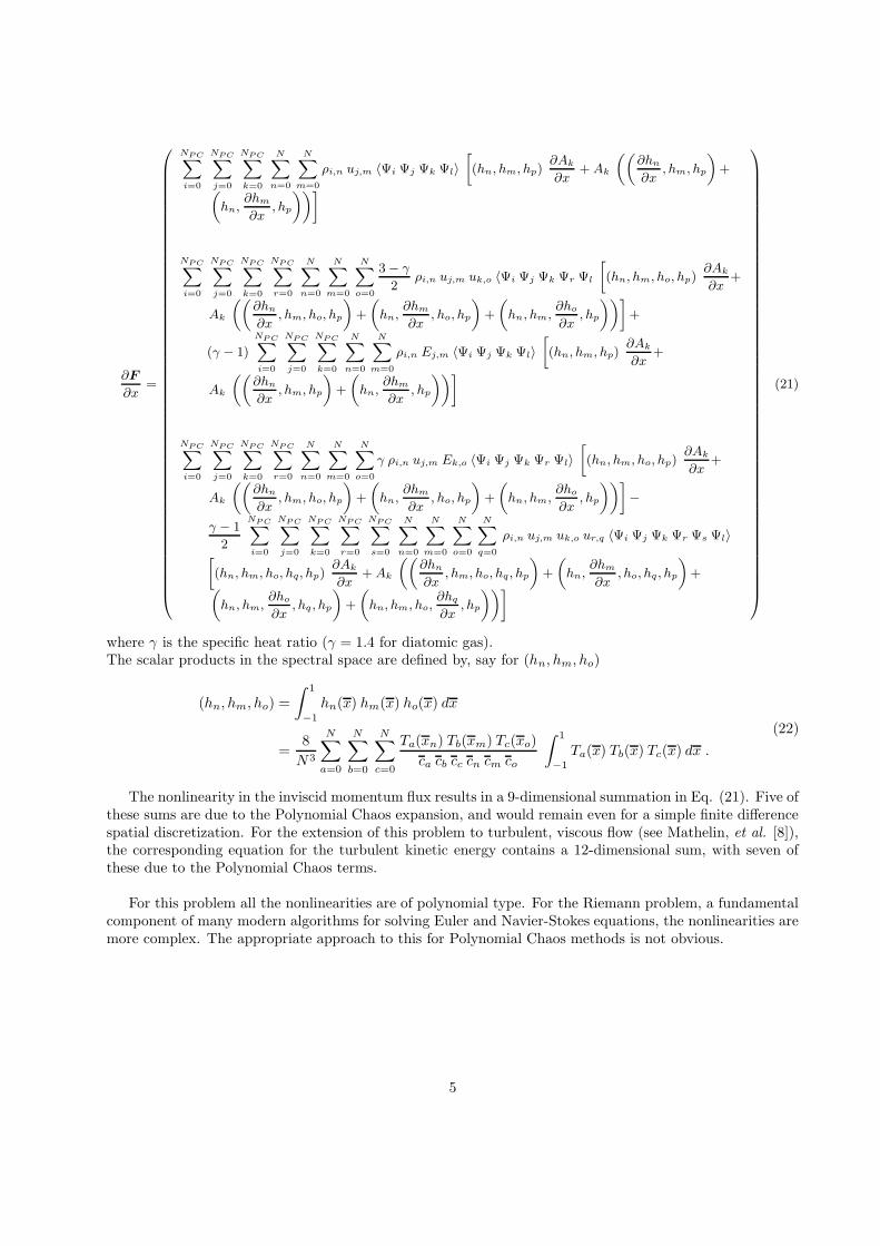
The nonlinearity in the inviscid momentum flux results in a 9-dimensional summation in Eq. (21). Five ofthese sums are due to the Polynomial Chaos expansion, and would remain even for a simple finite differencespatial discretization. For the extension of this problem to turbulent, viscous flow (see Mathelin, et al. [8]),the corresponding equation for the turbulent kinetic energy contains a 12-dimensional sum, with seven ofthese due to the Polynomial Chaos terms.

For this problem all the nonlinearities are of polynomial type. For the Riemann problem, a fundamentalcomponent of many modern algorithms for solving Euler and Navier-Stokes equations, the nonlinearities aremore complex. The appropriate approach to this for Polynomial Chaos methods is not obvious.

5

3 Stochastic Collocation Method

The stochastic collocation method was developed to enable application to Spectral Discontinuous GalerkinMethods (for which solution of the Riemann problem is a necessity) as well as to reduce the cost of PolynomialChaos methods for more classical discretizations, such as described above for quasi 1-D nozzle flow.

Let a and b be two independent random variables. In the Polynomial Chaos method, the infinite seriesfor each variable would be expressed as, say, for a,

a =

∞∑

i=0

aiΨi(ξ) , (23)

and the product ab would be

ab =∞∑

i=0

∞∑

j=0

aibjΨi(ξ)Ψj(ξ) . (24)

(Here we drop any dependence upon x and t and concentrate on just the random variable ξ without referenceto the random event parameter θ.)

The finite series for a is then

a =

NP C∑

i=0

aiΨi(ξ) . (25)

The usual Galerkin truncation yields for the expansion coefficients of the product c = ab

(ab)k =

NP C∑

i=0

NP C∑

j=0

ai bj 〈Ψi Ψj Ψk〉 ∀k ∈ [0; NPC ] ⊂ N . (26)

Therefore, computing the NPC + 1 coefficients of the product ab takes of order N 3

PC operations. Thecomplexity is even greater for cubic products. Moreover, for non-polynomial nonlinearities, such as thosethat arise in the Riemann problem, the Galerkin truncation is not obvious.

For traditional deterministic problems, these difficulties are often treated by resorting to a collocationmethod instead of the Galerkin method. The usual spatial collocation approach consists of projecting theequations into the physical space (x). But a “physical space” corresponding to the random variable ξ haslimited physical meaning, and the spatial scheme cannot be directly transformed. To deal with this problem,we define a new stochastic space whose properties are known.

In the stochastic collocation method (SCM) one lets the Probability Density Function (PDF) of therandom variable ξ serve as the basis for the transformation between the physical random variable ξ andits artificial stochastic space. We use α to denote a point in this artificial stochastic space. The range ofthe corresponding Cumulative Distribution Function (CDF) is [0,1], and provided that the underlying PDFis non-zero in the interior of its domain, the CDF is strictly monotonic and therefore this transformationis bijective. Denote the CDF of ξ by Fξ(ξ). We prefer to map the CDF to the standard domain [-1,1] oforthogonal polynomials, and so we define

Fξ(ξ) = 2Fξ(ξ) − 1 . (27)

Finally, denote the inverse of Fξ by Gξ. Let α be a point in the domain [-1,1] of G. This is the new, knownstochastic space that is the foundation of the SCM. We have then

α = Fξ(ξ) = 2Fξ(ξ)− 1 (28)

andξ = Gξ(α) . (29)

The SCM utilizes collocation points αi, i = 0, . . . , Nq, in [-1,1] . These have associated quadrature weightswi, chosen to give the best approximation to inner products on [-1,1]. In the present work we make the

6

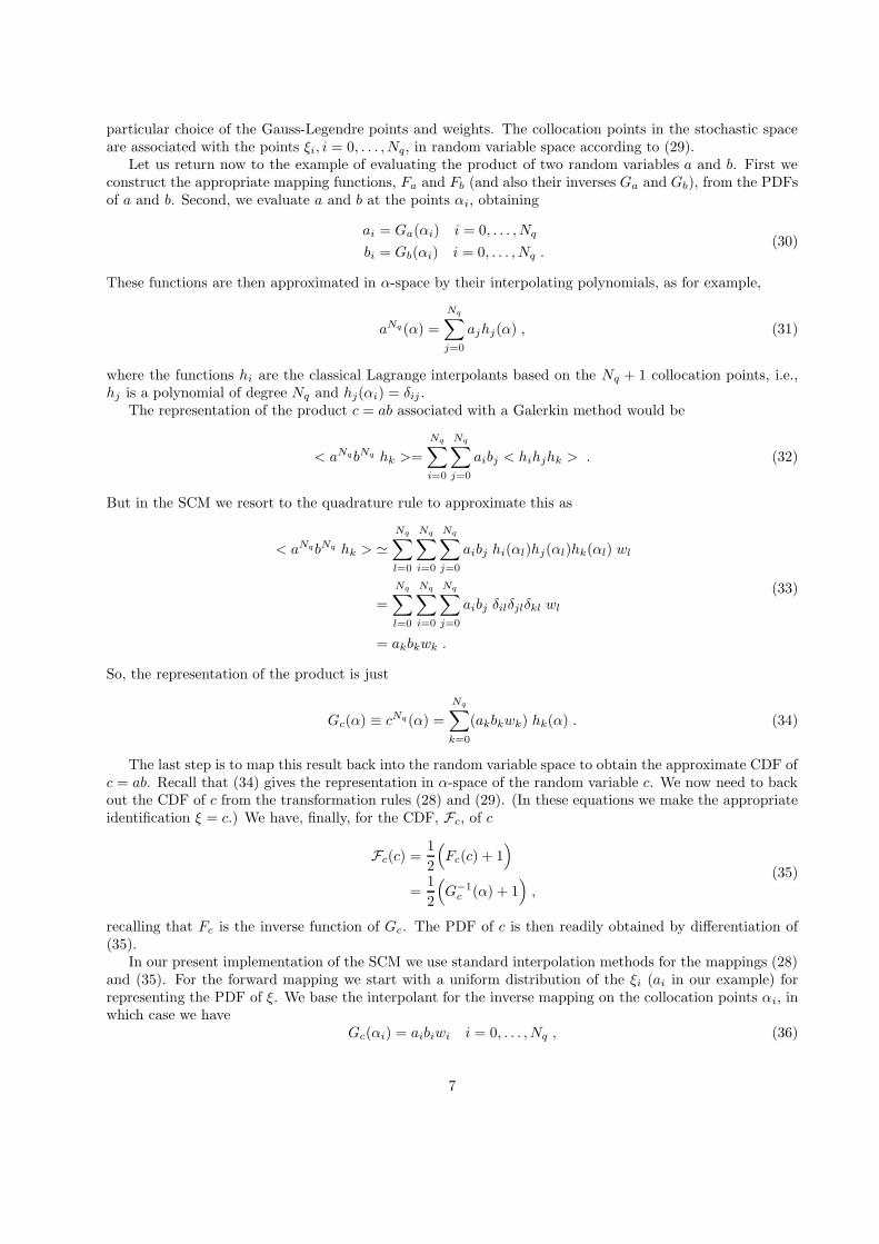
particular choice of the Gauss-Legendre points and weights. The collocation points in the stochastic spaceare associated with the points ξi, i = 0, . . . , Nq, in random variable space according to (29).

Let us return now to the example of evaluating the product of two random variables a and b. First weconstruct the appropriate mapping functions, Fa and Fb (and also their inverses Ga and Gb), from the PDFsof a and b. Second, we evaluate a and b at the points αi, obtaining

ai = Ga(αi) i = 0, . . . , Nq

bi = Gb(αi) i = 0, . . . , Nq .(30)

These functions are then approximated in α-space by their interpolating polynomials, as for example,

aNq (α) =

Nq∑

j=0

ajhj(α) , (31)

where the functions hi are the classical Lagrange interpolants based on the Nq + 1 collocation points, i.e.,hj is a polynomial of degree Nq and hj(αi) = δij .

The representation of the product c = ab associated with a Galerkin method would be

< aNqbNq hk >=

Nq∑

i=0

Nq∑

j=0

aibj < hihjhk > . (32)

But in the SCM we resort to the quadrature rule to approximate this as

< aNqbNq hk > 'Nq∑

l=0

Nq∑

i=0

Nq∑

j=0

aibj hi(αl)hj(αl)hk(αl) wl

=

Nq∑

l=0

Nq∑

i=0

Nq∑

j=0

aibj δilδjlδkl wl

= akbkwk .

(33)

So, the representation of the product is just

Gc(α) ≡ cNq (α) =

Nq∑

k=0

(akbkwk) hk(α) . (34)

The last step is to map this result back into the random variable space to obtain the approximate CDF ofc = ab. Recall that (34) gives the representation in α-space of the random variable c. We now need to backout the CDF of c from the transformation rules (28) and (29). (In these equations we make the appropriateidentification ξ = c.) We have, finally, for the CDF, Fc, of c

Fc(c) =1

2

(

Fc(c) + 1)

=1

2

(

G−1

c (α) + 1)

,

(35)

recalling that Fc is the inverse function of Gc. The PDF of c is then readily obtained by differentiation of(35).

In our present implementation of the SCM we use standard interpolation methods for the mappings (28)and (35). For the forward mapping we start with a uniform distribution of the ξi (ai in our example) forrepresenting the PDF of ξ. We base the interpolant for the inverse mapping on the collocation points αi, inwhich case we have

Gc(αi) = aibiwi i = 0, . . . , Nq , (36)

7

since hk(αi) = δik.The complexity of this implementation of the SCM in one dimension is Nq, regardless of the form of the

nonlinearity. In contrast the Galerkin method already scales as N 3

PC for a simple quadratic nonlinearity.The quadrature in the stochastic collocation method does introduce additional errors compared with thoseof the Galerkin method, but these are reduced as Nq increases. This is usually not a major issue since thecollocation scheme allows for dramatic speed-up compared to full Galerkin approach and a relatively highvalue for Nq is affordable.

As an example of this process, consider the cubic equation

f(u) = u3 , (37)

where u is a Gaussian random variable, with mean 1.0 and standard deviation of 1/(2√

π. Figure 1 showsthe PDF of u, the α-representation of u, the α-representation of f(u) = u3, and the corresponding PDF off(u).

(a) PDF of input function u. (b) Projection of the input function into the α-space.

(c) Output function f(u) in the α-space (d) PDF of output function f(u).

Figure 1: Illustration of stochastic collocation for f(u) = u3.

8

4 Application to Stochastic Riemann Solver

To illustrate the applicability of the above method, the stochastic Riemann problem is considered here. Thefield variables are assumed to be discontinuous at a time t and this leads to the generation of shock wave,rarefaction and expansion fan. See Landau & Lifshitz ([5]) or Liepmann & Roshko ([6]) for a review ofthe physical phenomena involved. To compute the resulting state for later times, one can make use of thealgorithm proposed by Sod ([10]). It produces strongly non-linear equations including rational powers andconditional expressions. While straightforward in a deterministic space, the application of such an algorithmbecomes very tricky with a stochastic approach. For example, two expressions are to be applied dependingon the pressure ratio: if P ∗/P > 1 , then use equation (a) and if P ∗/P < 1, then use equation (b). Butwhen both pressures are non-deterministic, what does P ∗/P > 1 or P ∗/P < 1 mean ?

Using the collocation scheme, the pressure ratio now has a deterministic expression in the α-space andit is possible to determine the resulting state. Figures 2 through 4 show the propagation of the stochasticdescription of the state across the discontinuity, i.e., the stochastic collocation solution of the stochasticRiemann problem. In these computations Nq = 200.

(a) Left state. (b) Interface state. (c) Right state.

Figure 2: Density PDF evolution throughout a discontinuity.

(a) Left state. (b) Interface state. (c) Right state.

Figure 3: Velocity PDF evolution throughout a discontinuity.

Preliminary results from Mathelin, et al. ([8]) indicate that substantial CPU savings have been achievedby the stochastic collocation method in Polynomial Chaos solutions of quasi 1-D nozzle flow. In their simplestcase, Euler flow, the computational time was reduced by a factor of 4. The computational savings is stronglydependent upon the discretization parameters. More details are available in [8].

9

(a) Left state. (b) Interface state. (c) Right state.

Figure 4: Pressure PDF evolution throughout a discontinuity.

5 Acknowlegments

The authors thank Thomas A. Zang for suggesting this problem and for his support.

References

[1] H. W. Coleman and F. Stern, Uncertainties and CFD code validation, J. Fluids Eng., 119 (1997),pp. 795–803.

[2] R. G. Ghanem and P. D. Spanos, Stochastic finite elements: a spectral approach, Springer-Verlag,New-York, 1991.

[3] L. Huyse, Free-form airfoil shape optimization under uncertainty using maximum expected value and

second-order second-moment strategies, ICASE Report No. 2001–18, 2001.

[4] U. B. Mehta, Some aspects of uncertainty in computational fluid dynamics results, J. Fluids Eng.,113 (1991), pp. 538–543.

[5] L. D. Landau and E. M. Lifshitz, Course of theoretical physics. Vol.6. Fluid mechanics, Pergamonpress, Oxford, 1982.

[6] H. W. Liepmann and A. Roshko, Elements of gas dynamics, Wiley, New-York, 1957.

[7] L. Mathelin and M. Y. Hussaini, Uncertainty quantification in CFD simulations: a stochastic

spectral approach, 2nd International Conference on Computational Fluid Dynamics, Sydney, Australia,July 15-19, 2002.

[8] L. Mathelin, M. Y. Hussaini, T. A. Zang and F. Bataille, Uncertainty propagation for turbulent,

compressible flow in a quasi-1D nozzle using polynomial chaos, AIAA-2003-4240, 16th AIAA CFDConference, Orlando, FL, June 23-26, 2003.

[9] P.J. Roache, Perspective: a method for uniform reporting of grid refinements studies, J. Fluids Eng.,116 (1994), pp. 405–413.

[10] G. A. Sod, A survey of several finite difference methods for systems of nonlinear hyperbolic conservation

laws, J. Comput. Phys., 27 (1978), pp. 1–31.

[11] A. C. Taylor, L. L. Green, P. A. Newman and M. M. Putko, Some advanced concepts in

discrete aerodynamic sensitivity analysis, AIAA-2001-2529, 2001.

10

[12] R. W. Walters and L. Huyse, Uncertainty analysis for fluid mechanics with applications, ICASEReport No. 2002-1, 2002.

[13] N. Wiener, The homogeneous chaos, Amer. J. Math., 60 (1938), pp. 897–936.

[14] D. Xiu, D. Lucor, C.-H. Su and G. Em. Karniadakis, Stochastic modeling of flow-structure

interactions using generalized polynomial chaos, J. Fluids Eng., 124(1) (2002), pp. 51–59.

[15] D. Xiu and G. Em. Karniadakis, The Wiener-Askey polynomial chaos for stochastic differential

equations, SIAM J. Sci. Comput. 24(2), (2002), pp. 619–644.

[16] D. Xiu D. and G. Em. Karniadakis, Modeling uncertainty in flow simulations via generalized

polynomial chaos, J. Comput. Phys. (2002), to appear.

[17] H. C. Yee and P. K. Sweby, Aspects of numerical uncertainties in time marching to steady-state

numerical solutions, AIAA J., 36(5) (1998), pp. 712–724.

11

REPORT DOCUMENTATION PAGE Form ApprovedOMB No. 0704–0188

The public reporting burden for this collection of information is estimated to average 1 hour per response, including the time for reviewing instructions, searching existing data sources,gathering and maintaining the data needed, and completing and reviewing the collection of information. Send comments regarding this burden estimate or any other aspect of this collectionof information, including suggestions for reducing this burden, to Department of Defense, Washington Headquarters Services, Directorate for Information Operations and Reports(0704-0188), 1215 Jefferson Davis Highway, Suite 1204, Arlington, VA 22202-4302. Respondents should be aware that notwithstanding any other provision of law, no person shall besubject to any penalty for failing to comply with a collection of information if it does not display a currently valid OMB control number.PLEASE DO NOT RETURN YOUR FORM TO THE ABOVE ADDRESS.

Standard Form 298 (Rev. 8/98)Prescribed by ANSI Std. Z39.18

1. REPORT DATE (DD-MM-YYYY)02-2003

2. REPORT TYPEContractor Report

3. DATES COVERED (From - To)

4/2002–12/2002

4. TITLE AND SUBTITLE

A Stochastic Collocation Algorithm for Uncertainty Analysis

5a. CONTRACT NUMBER

5b. GRANT NUMBER

5c. PROGRAM ELEMENT NUMBER

5d. PROJECT NUMBERNCC1-02025

5e. TASK NUMBER

5f. WORK UNIT NUMBER706-20-61-01

6. AUTHOR(S)

Lionel Mathelin and M. Yousuff Hussaini

7. PERFORMING ORGANIZATION NAME(S) AND ADDRESS(ES)Florida State University

Tallahassee, Florida 32306-4120

8. PERFORMING ORGANIZATIONREPORT NUMBER

9. SPONSORING/MONITORING AGENCY NAME(S) AND ADDRESS(ES)National Aeronautics and Space Administration

Washington, DC 20546-0001

10. SPONSOR/MONITOR’S ACRONYM(S)NASA

11. SPONSOR/MONITOR’S REPORTNUMBER(S)

NASA/CR–2003–212153

12. DISTRIBUTION/AVAILABILITY STATEMENT

Unclassified-UnlimitedSubject Category 64Availability: NASA CASI (301) 621-0390 Distribution: Standard

13. SUPPLEMENTARY NOTES

An electronic version can be found at http://techreports.larc.nasa.gov/ltrs/ or http://techreports.larc.nasa.gov/cgi-bin/NTRS.Langley Technical Monitor: Thomas A. Zang

14. ABSTRACT

This report describes a stochastic collocation method to adequately handle a physically intrinsic uncertainty in the variables of anumerical simulation. For instance, while the standard Galerkin approach to Polynomial Chaos requires multi-dimensional summationsover the stochastic basis functions, the stochastic collocation method enables to collapse those summations to a one-dimensionalsummation only. This report furnishes the essential algorithmic details of the new stochastic collocation method and provides as anumerical example the solution of the Riemann problem with the stochastic collocation method used for the discretization of thestochastic parameters.

15. SUBJECT TERMS

uncertainty, stochastic, probabilistic

16. SECURITY CLASSIFICATION OF:

a. REPORT

U

b. ABSTRACT

U

c. THIS PAGE

U

17. LIMITATION OFABSTRACT

UU

18. NUMBEROFPAGES

16

19a. NAME OF RESPONSIBLE PERSON

STI Help Desk (email: help@sti.nasa.gov)

19b. TELEPHONE NUMBER (Include area code)

(301) 621-0390