A State-Space Approach to Control ofInterconnected Systems

Part I: Spatially Invariant Systems

Cédric Langbort 1 Raffaello D’Andrea 2

1Center for the Mathematics of InformationCALIFORNIA INSTITUTE OF TECHNOLOGY

2Department of Mechanical & Aerospace EngineeringCORNELL UNIVERSITY

with contributions from: Ramu Chandra, Jeff Fowler, Ben Recht

Workshop on “Control, estimation, and optimization ofinterconnected systems: from theory to industrial applications”

CDC-ECC ’05, Sevilla, Spain

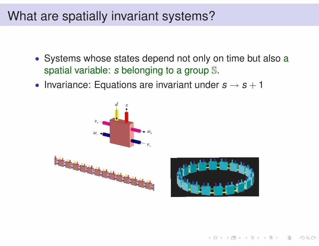
What are spatially invariant systems?

• Systems whose states depend not only on time but also aspatial variable: s belonging to a group S.

• Invariance: Equations are invariant under s → s + 1

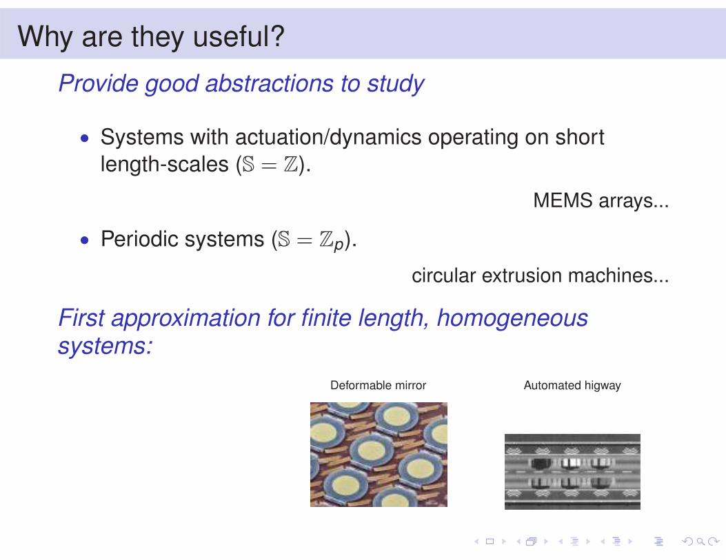
Why are they useful?

Provide good abstractions to study

• Systems with actuation/dynamics operating on shortlength-scales (S = Z).

MEMS arrays...

• Periodic systems (S = Zp).

circular extrusion machines...

First approximation for finite length, homogeneoussystems:

Deformable mirror Automated higway

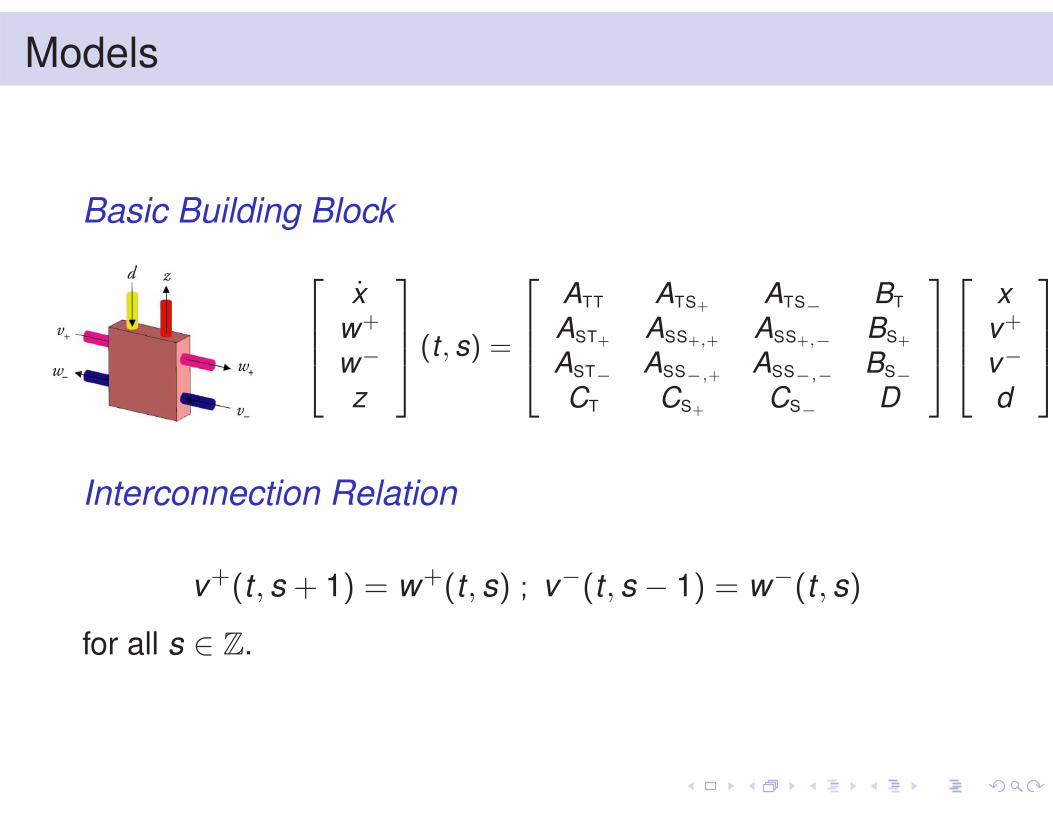
Models

Basic Building Block

⎡⎢⎢⎣

xw+

w−

z

⎤⎥⎥⎦ (t , s) =

⎡⎢⎢⎣

ATT ATS+ ATS− BT

AST+ ASS+,+ ASS+,− BS+

AST− ASS−,+ ASS−,− BS−CT CS+ CS− D

⎤⎥⎥⎦

⎡⎢⎢⎣

xv+

v−

d

⎤⎥⎥⎦

Interconnection Relation

v+(t , s + 1) = w+(t , s) ; v−(t , s − 1) = w−(t , s)

for all s ∈ Z.

Models

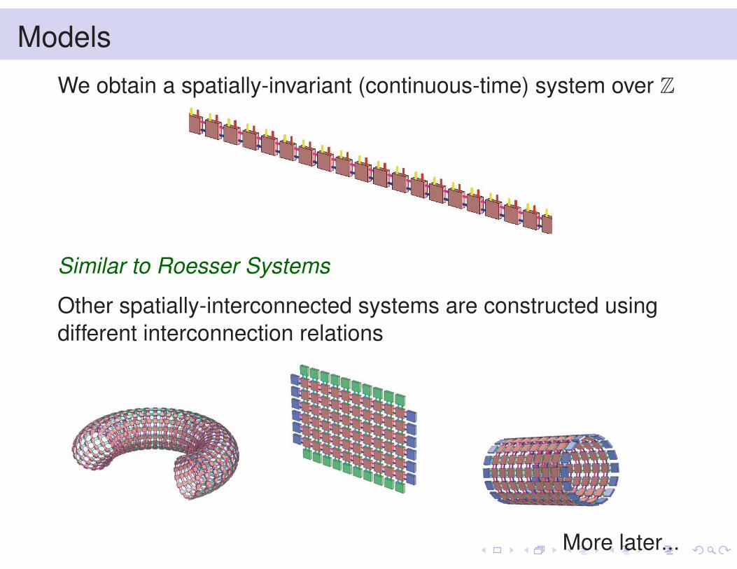
We obtain a spatially-invariant (continuous-time) system over Z

Similar to Roesser Systems

Other spatially-interconnected systems are constructed usingdifferent interconnection relations

More later...

Control goals

We want to ensure• Well-posedness: interconnection signals v±, w± have

finite norms.• Stability: |x(t)| ≤ e−αt |x(0)| for α > 0.• Performance: ‖z‖ < ‖d‖.

where

|x(t)| =∞∑

s=−∞x(t , s)∗x(t , s) ; ‖z‖ =

∫ ∞

0|z(t)|dt

InspirationMain Idea

Treat spatially-invariant systems as interconnection in theRobust Control/ LFT framework.

InspirationProving discrete-time KYP via µ-analysis methods

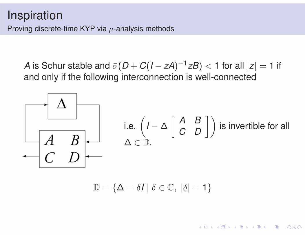
A is Schur stable and σ(D + C(I − zA)−1zB) < 1 for all |z| = 1 ifand only if the following interconnection is well-connected

i.e.(

I − ∆

[A BC D

])is invertible for all

∆ ∈ D.

D = {∆ = δI | δ ∈ C, |δ| = 1}

InspirationProving discrete-time KYP via µ-analysis methods

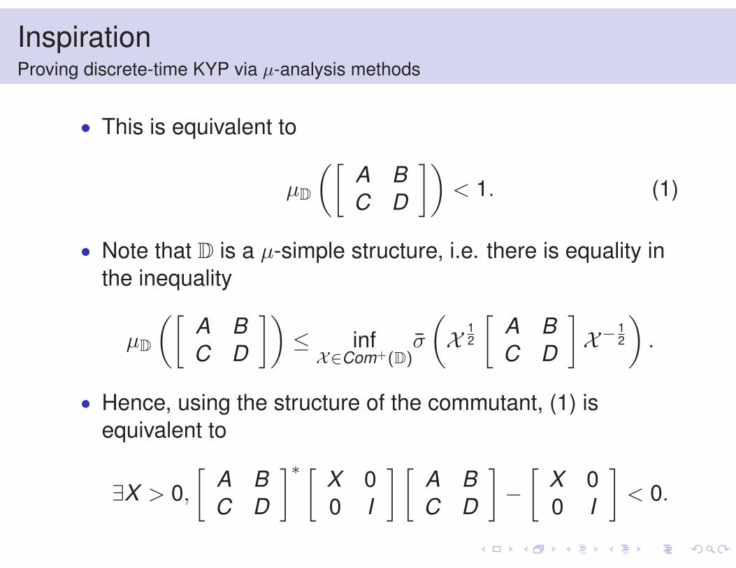
• This is equivalent to

µD

([A BC D

])< 1. (1)

• Note that D is a µ-simple structure, i.e. there is equality inthe inequality

µD

([A BC D

])≤ inf

X∈Com+(D)σ

(X 1

2

[A BC D

]X− 1

2

).

• Hence, using the structure of the commutant, (1) isequivalent to

∃X > 0,

[A BC D

]∗ [X 00 I

] [A BC D

]−

[X 00 I

]< 0.

Extension to spatially invariant systems

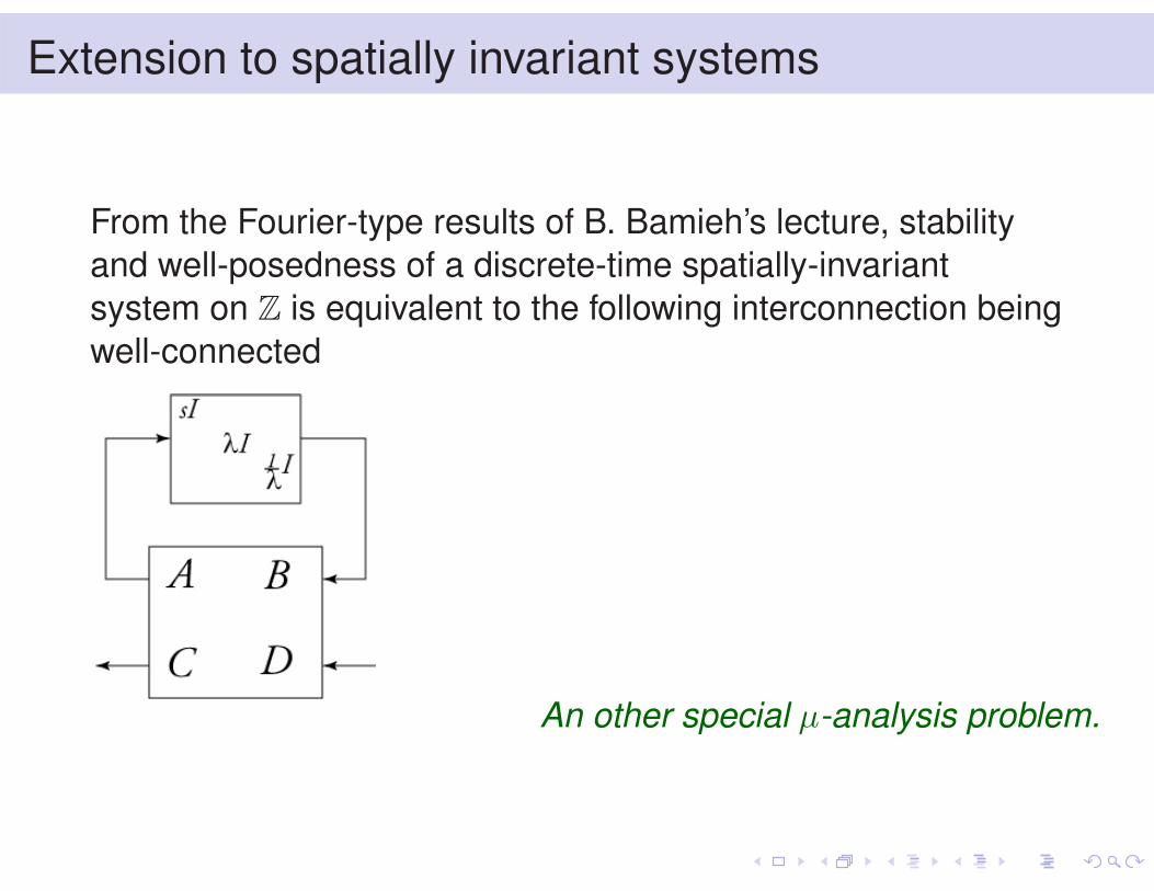
From the Fourier-type results of B. Bamieh’s lecture, stabilityand well-posedness of a discrete-time spatially-invariantsystem on Z is equivalent to the following interconnection beingwell-connected

An other special µ-analysis problem.

Stability of spatially invariant systems

• Question reduces to:“When is

⎛⎝I −

⎡⎣ sI 0 0

0 λI 00 0 λ−1I

⎤⎦

⎡⎣ ATT ATS+ ATS−

AST+ ASS+,+ ASS+,−AST− ASS−,+ ASS−,−

⎤⎦

⎞⎠

invertible for all |s| < 1, |λ| = 1 ? ”

• Ultimately:

“When is(

I −[

λI 00 1

λ I

] [ASS+,+ ASS+,−ASS−,+ ASS−,−

])invertible

for all |λ| = 1?”

Stability of spatially invariant systemsA lemma

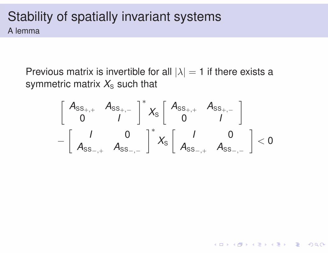
Previous matrix is invertible for all |λ| = 1 if there exists asymmetric matrix XS such that

[ASS+,+ ASS+,−

0 I

]∗XS

[ASS+,+ ASS+,−

0 I

]

−[

I 0ASS−,+ ASS−,−

]∗XS

[I 0

ASS−,+ ASS−,−

]< 0

Stability of spatially invariant systemsA lemma

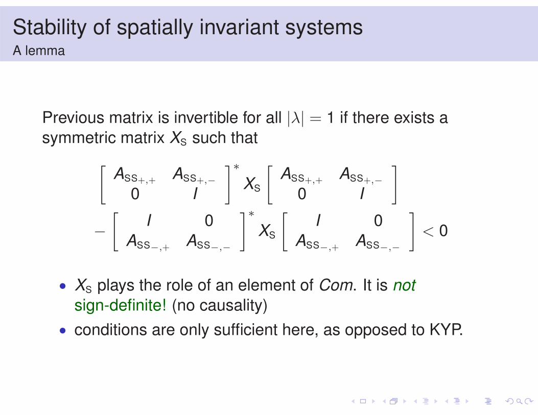
Previous matrix is invertible for all |λ| = 1 if there exists asymmetric matrix XS such that

[ASS+,+ ASS+,−

0 I

]∗XS

[ASS+,+ ASS+,−

0 I

]

−[

I 0ASS−,+ ASS−,−

]∗XS

[I 0

ASS−,+ ASS−,−

]< 0

• XS plays the role of an element of Com. It is notsign-definite! (no causality)

• conditions are only sufficient here, as opposed to KYP.

Stability of spatially invariant systemsAn example

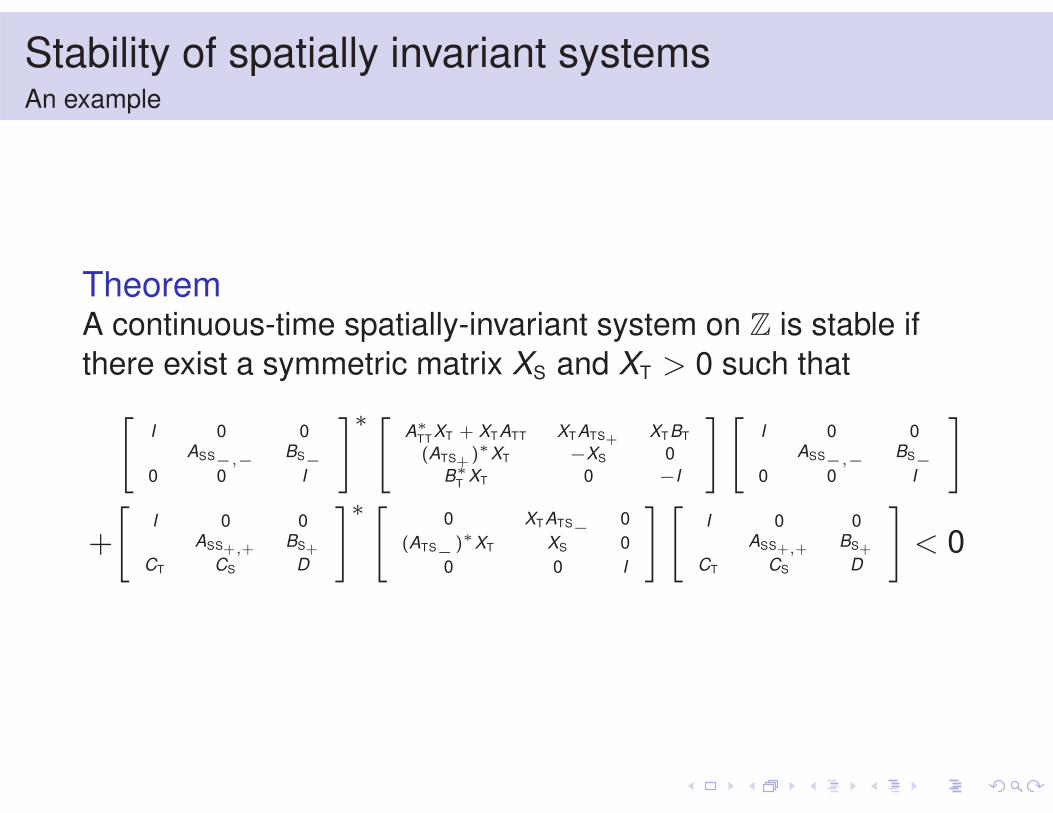
TheoremA continuous-time spatially-invariant system on Z is stable ifthere exist a symmetric matrix XS and XT > 0 such that

[I 0 0

ASS−,− BS−0 0 I

]∗ [A∗

TTXT + XTATT XTATS+ XTBT

(ATS+ )∗XT −XS 0B∗

T XT 0 −I

] [I 0 0

ASS−,− BS−0 0 I

]

+

[I 0 0

ASS+,+ BS+CT CS D

]∗ [0 XTATS− 0

(ATS− )∗XT XS 00 0 I

] [I 0 0

ASS+,+ BS+CT CS D

]< 0

Control Synthesis

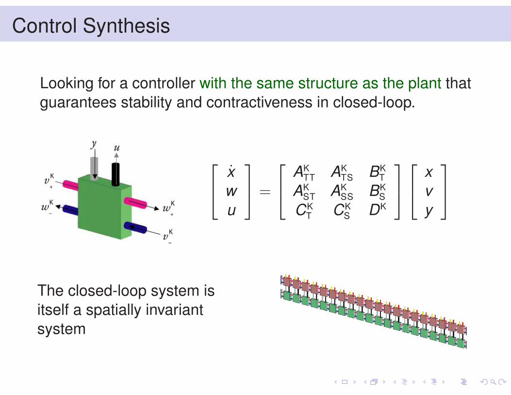
Looking for a controller with the same structure as the plant thatguarantees stability and contractiveness in closed-loop.

⎡⎣ x

wu

⎤⎦ =

⎡⎣ AK

TT AKTS BK

T

AKST AK

SS BKS

CKT CK

S DK

⎤⎦

⎡⎣ x

vy

⎤⎦

The closed-loop system isitself a spatially invariantsystem

Control SynthesisSeveral steps

For the continuous-time spatially-invariant system on Z

1. Apply analysis LMIs to the closed-loop system: obtainBMIs

Control SynthesisSeveral steps

For the continuous-time spatially-invariant system on Z

1. Apply analysis LMIs to the closed-loop system: obtainBMIs

2. Apply a Bilinear Algebraic Transformation (β = 1−λ1+λ ) to the

closed-loop system: BMIs have the same form as in theusual continuous-time synthesis problem.

Control SynthesisSeveral steps

For the continuous-time spatially-invariant system on Z

1. Apply analysis LMIs to the closed-loop system: obtainBMIs

2. Apply a Bilinear Algebraic Transformation (β = 1−λ1+λ ) to the

closed-loop system: BMIs have the same form as in theusual continuous-time synthesis problem.

3. Convexify using classical projection lemmas (modulo theabsence of sign-definiteness in the scales) [Gahinet &Apkarian, Packard]: BMIs are equivalent to LMIs. Atransformed controller K is obtained

Control SynthesisSeveral steps

For the continuous-time spatially-invariant system on Z

1. Apply analysis LMIs to the closed-loop system: obtainBMIs

2. Apply a Bilinear Algebraic Transformation (β = 1−λ1+λ ) to the

closed-loop system: BMIs have the same form as in theusual continuous-time synthesis problem.

3. Convexify using classical projection lemmas (modulo theabsence of sign-definiteness in the scales) [Gahinet &Apkarian, Packard]: BMIs are equivalent to LMIs. Atransformed controller K is obtained

4. To reconstruct controller, apply the “inverse” of the BAT toK , making sure to obtain an implementable controller

Summary

We have obtained convex controller synthesis conditions forspatially-invariant systems (over Z)

• A single LMI to solve, involving only the basic buildingblock, even though problem is infinite-dimensional(compare the necessary and sufficient Riccati equations inB. Bamieh’s talk)

• Controller has the same structure as the plant• No conservatism added at the controller synthesis level

Generalizations

• Straightforward extension to system over ZN , N > 1.

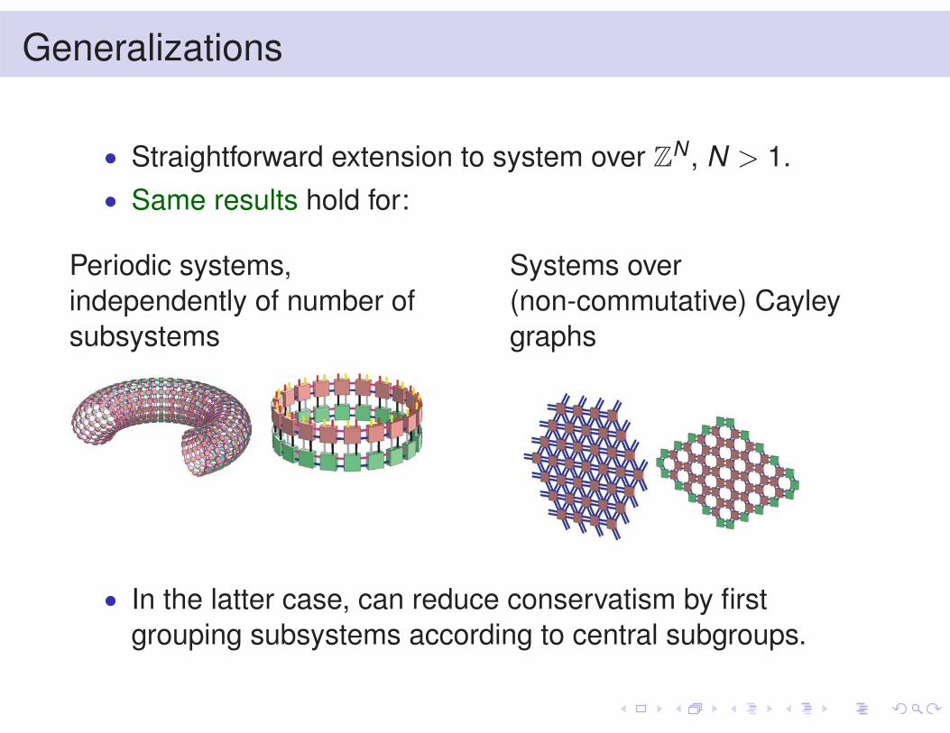
• Same results hold for:

Periodic systems,independently of number ofsubsystems

Systems over(non-commutative) Cayleygraphs

• In the latter case, can reduce conservatism by firstgrouping subsystems according to central subgroups.

Generalizations-IISome boundary conditions

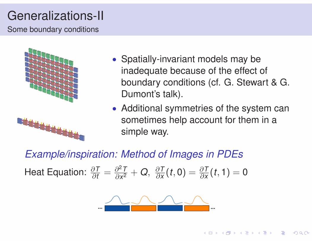
• Spatially-invariant models may beinadequate because of the effect ofboundary conditions (cf. G. Stewart & G.Dumont’s talk).

• Additional symmetries of the system cansometimes help account for them in asimple way.

Example/inspiration: Method of Images in PDEs

Heat Equation: ∂T∂t = ∂2T

∂x2 + Q, ∂T∂x (t , 0) = ∂T

∂x (t , 1) = 0

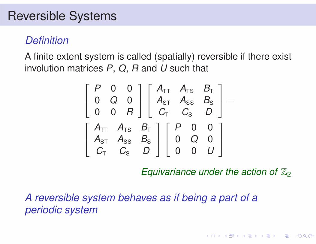
Reversible Systems

DefinitionA finite extent system is called (spatially) reversible if there existinvolution matrices P, Q, R and U such that

⎡⎣ P 0 0

0 Q 00 0 R

⎤⎦

⎡⎣ ATT ATS BT

AST ASS BS

CT CS D

⎤⎦ =

⎡⎣ ATT ATS BT

AST ASS BS

CT CS D

⎤⎦

⎡⎣ P 0 0

0 Q 00 0 U

⎤⎦

Equivariance under the action of Z2

A reversible system behaves as if being a part of aperiodic system

Reversible systemsResults

Analysis

If the periodic extension is stable and contractive, then so is thecorresponding reversible finite extent system.

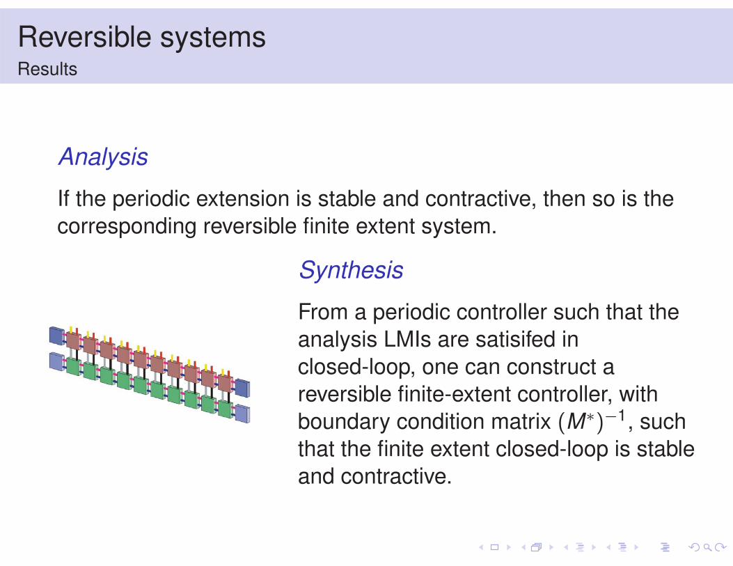
Synthesis

From a periodic controller such that theanalysis LMIs are satisifed inclosed-loop, one can construct areversible finite-extent controller, withboundary condition matrix (M∗)−1, suchthat the finite extent closed-loop is stableand contractive.

Application exampleClose formation flight

• Each aircraft’s wake influences itsimmediate follower, (hopefully)diminishing its drag.

• System can be modeled as achained spatially-interconnectedsystem, to which preceding resultsare applicable (approximatingpropagation delays)

Application exampleClose formation flight

• Each aircraft’s wake influences itsimmediate follower, (hopefully)diminishing its drag.

• System can be modeled as achained spatially-interconnectedsystem, to which preceding resultsare applicable (approximatingpropagation delays)

Experimental results for a formation of 10 identical wings,applying a disturbance at each wing. z(t , s) is yaw at s.

Controller RMS Gain Gain at rear pairdistributed 0.37 0.35

decentralized 3.15 3.13

Synthesizing the best (centralized) controller is toocomputationally intensive

Afternoon talk

• Heterogenous subsystems on arbitrary graphs• Conservatism/ non-ideal interconnection relations• Numerical Methods...

Some references I

R. D’Andrea & G. DullerudDistributed Control Design for Spatially InterconnectedSystemsIEEE Transactions on Automatic Control, vol. 48, no. 9,September 2003.

C.L. & R. D’AndreaDistributed Control of Spatially Reversible InterconnectedSystems with Boundary ConditionsSIAM Journal on Control and Optimization, vol. 44, no. 1,pp. 1-28, 2005.