ARTICLE IN PRESS

0925-2312/$ - se

doi:10.1016/j.ne

�Tel.: +353 1

E-mail addr

Neurocomputing 70 (2006) 513–524

www.elsevier.com/locate/neucom

A set of nonlinear equations and inequalities arising in roboticsand its online solution via a primal neural network

Yunong Zhang�

Hamilton Institute, National University of Ireland at Maynooth, Maynooth, Co. Kildare, Ireland

Received 10 January 2005; received in revised form 25 November 2005; accepted 30 November 2005

Communicated by F.A. Mussa-Ivaldi

Available online 12 May 2006

Abstract

In this paper, for handling general minimum-effort inverse-kinematic problems, the nonuniqueness condition is investigated. A set of

nonlinear equations and inequality is presented for online nonuniqueness-checking. The concept and utility of primal neural networks

(NNs) are introduced in this context of dynamical inequalities and constraints. The proposed primal NN can handle well such a

nonlinear online-checking problem in the form of a set of nonlinear equations and inequality. Numerical examples demonstrate the

effectiveness and advantages of the primal NN approach.

r 2006 Elsevier B.V. All rights reserved.

Keywords: Minimum effort inverse kinematics; Nonuniqueness; Discontinuity; Nonlinear equations and inequalities; Primal neural network

1. Introduction

Redundant manipulators are robots having more de-grees-of-freedom (DOF) than required to perform a givenend-effector task [15]. Our human arm is also such aredundant system [8]. One fundamental issue in operatingsuch systems is the redundancy-resolution problem[25,29,30]. By resolving the redundancy, the robots canavoid obstacles, joint physical limits, as well as to optimizevarious performance criteria. In addition to minimum-energy redundancy resolution [15,25,30], another interest-ing approach is the minimum-effort redundancy resolution[3,5,9,16,31]. The minimum-effort resolution may encoun-ter discontinuities due to the nonuniqueness of the solutionat some time instants [6]. The nonuniqueness of theminimum-effort solution was previously checked by ageometrical method [6]. As shown in this paper, thenonuniqueness can be checked more generally andefficiently by solving online a set of nonlinear equationsand inequalities.

e front matter r 2006 Elsevier B.V. All rights reserved.

ucom.2005.11.006

7084534; fax: +353 17086269.

ess: ynzhang@ieee.org.

It is worth mentioning that in view of its fundamentalrole arising in numerous fields of science and engineering,the problem of solving groups of linear equations andinequalities has been investigated extensively for the pastdecades. For example, about the recent research based onrecurrent neural networks (NNs) (specifically, the Hop-field-type NNs), see [2,10,11,18,19,21,26,27] and thereferences therein. The NN approach is now thought tobe a powerful tool for online solutions, in light of itsparallel distributed computing nature and hardwareimplementability [1,4,13,19].In the aforementioned literature, most researches are

devoted to solving linear equations and inequalities only(with the matrix-inverse problem as a special case). Amongthem, the mathematical description can be unified asEypf , Cy ¼ g where y is the unknown vector to bedetermined, given coefficient matrices E, C and coefficientvectors f, g. In the group of linear equations andinequalities, Cy ¼ g defines the problem to be solved whileEypf defines its constraints. To our best knowledge, therehave been few research results about solving nonlinear orhybrid equations/inequalities based on NN approaches. Onthe other hand, the nonlinear situations are encounteredin the minimum-effort redundancy resolution of robot

ARTICLE IN PRESSY. Zhang / Neurocomputing 70 (2006) 513–524514

manipulators. The set of such nonlinear equations andinequalities is in the form of Eypf , Cy ¼ g and yTy ¼ h

with given scalar h40. The real-time computation require-ment becomes stringent, especially for sensor-based roboticsystems of high DOF.

The design methods and techniques for recurrent NNsare briefly reviewed as follows. In terms of the types ofdecision variables involved, the NN models can be dividedinto two classes: the pure primal NNs and the nonprimalNNs. In detail, we have the following concepts.

Concept 1: A recurrent NN is called primal NN, if thenetwork dynamic equation and implementation only usethe original (or to say, primal) decision variables, y. Forexample, the neural models in [2,19,27] are primal NNs.

Concept 2: A recurrent NN is called nonprimal NN, if thenetwork dynamic equation and implementation use anyauxiliary decision variables, in addition to the originalones. For example, the primal–dual NNs in [29,30], thedual NNs in [20,25], and the Lagrange NN in [22].

The earlier primal NN models such as [19] use finitepenalty parameters and generate approximate solutionsonly. By using auxiliary variables like dual decisionvariables, the nonprimal NNs usually have better conver-gence to exact/theoretical solutions as compared to primalNNs [20]. As the recent research shows [20,29], however,the primal NN is preferable in the context of dynamicconstraints/inequalities, provided that the solution accu-racy is acceptably good. In that case, the number ofconstraints/inequalities is dynamically changed, and thusthe hardware implementation of nonprimal NNs couldbecome less favorable, not to mention the networkcomplexity due to using auxiliary neurons.

In this paper, motivated by the above observations, wegeneralize the NN design experience to handling the non-linear/hybrid situations in minimum-effort robotics. Theconcept of primal NNs is thus formally proposed in solvingonline a set of nonlinear equations and inequalities. Theremainder of this paper is organized in four sections. Theproblem formulation is given in Section 2. The primal NN,together with convergence results, is presented in Section 3.Illustrative numerical examples are discussed in Section 4.Lastly, Section 5 concludes this paper with final remarks. Themain contributions of the paper are as follows:

(1)

Based on linear programming and equation-solving, amore efficient criterion is proposed for checkingnonuniqueness-points (as compared to geometricmethods).

(2)

The concept, utility and advantages of primal NNs areillustrated by developing a primal NN for such anonline-checking criterion of nonuniqueness (as com-pared to nonprimal NNs).

(3)

Previous robotic research results are confirmed by theconducted computer simulations and analysis. That is,nonuniqueness is nearly sufficient for the appearance ofdiscontinuities in the manipulators with low DOF/redundancy.

(4)

New robotic research results are summarized for themanipulators with high DOF/redundancy. That is,nonuniqueness is generally a necessary condition to theappearance of discontinuities in minimum-effortinverse-kinematic solutions.

2. Problem formulation

The minimum-effort redundancy resolution of robotmanipulators is the following infinity-norm minimizationproblem [3,9,16]:

minimize k_yk1 ð1Þ

subject to J _y ¼ _r, ð2Þ

y�pypyþ, ð3Þ

_y�p_yp_y

þ, ð4Þ

where y 2 Rn is the joint vector with physical limits ½y�; yþ�,_y 2 Rn is the joint-velocity vector with physical limits½_y�; _yþ�, and _r 2 Rm is the commanded Cartesian velocity

vector at the manipulator’s end-effector that can beplanned off-line or given in real time. The manipulatorJacobian matrix is an m� n rectangular matrix with mpn,and the infinity-norm of a vector is defined ask_yk1 ¼ max1pipnj

_yij.

Remark 1. It is worth mentioning here the significance ofthe minimum-effort redundancy resolution. As we know[3,31], the infinity-norm solution as in (1) minimizes thelargest component of joint velocity vector, and is thus moreconsistent with joint physical limits. In addition to such apursuit of low individual magnitude, the minimum-effortsolution could be used for even distribution of workload (ifjoint torque is minimized). As we also know [25,28], theminimum-energy redundancy resolution could be per-formed by minimizing the two norm of joint velocity/acceleration/torque. Being another scenario, the minimum-effort solution could complement such a research onmanipulators’ redundancy resolution. This may furtherprovide insights into human and animal motion controland diversity analysis. For example, why could we—human being—walk, run, and dance in different ways[7,8,23]? Like, sometimes with minimum-energy strategiesand sometimes with minimum-effort strategies?

2.1. Geometrical nonuniqueness-checking

Bound constraints (3) and (4) are incorporated here forthe avoidance of joint limits and joint velocity limits,respectively. In the geometrical method proposed in [6] forchecking the nonuniqueness, bound constraints (3) and (4)were not considered. It was shown there that a disconti-nuity point of minimum-effort solution appears because ofthe nonuniqueness of the solution at some time instants. Inother words, if the manipulator trajectory orients thesolution space so that it is parallel to a hypercube face

ARTICLE IN PRESSY. Zhang / Neurocomputing 70 (2006) 513–524 515

(which means the existence of multiple solutions), thesolution may jump from one edge/point to another insteadof continuing smoothly on its way [6].

This might be shown more clearly in Fig. 1, wherethe solution space is defined as S ¼ f_yjJ _y ¼ _rg. When Sis parallel to a cube face (here _y 2 R3 just for theconvenience of graphic interpretation), there exist mul-tiple solutions as shown in Fig. 1(a) via a bold line. WhenS is not parallel to the cube faces, there exists onlyone solution being the intersection of solution space Sand a cube face/edge, as shown in Fig. 1(b). As coeffi-cients J and _r change, the solution space S changesaccordingly (based on a member of multiple solutions).A jump might thus be generated from the previous solu-tion point to the current one. The magnitude of thejump depends on the distance between the two solutionpoints. The jump (which becomes a discontinuity point ifthe jump magnitude is large) happens because of thenonuniqueness of the solution point; specifically, from theexistence of multiple solutions to the existence of a uniquesolution or the existence of another set of multiplesolutions.

A measure of such a nonuniqueness point of theminimum-effort solution is computed by the followingzero subspace-angle method [6]. Define the nullspace of J

by N represented with a matrix N 2 Rn�ðn�mÞ such that theorthogonal columns of N span the nullspace. The subspaceangle n is defined as the angle between two hyperplanesembedded in a high-dimension space: nðS1;S2Þ ¼

cos�1ðminðdiagðSÞÞÞ with USVT ¼ ST1 S2 where subspaces

S1 and S2 are represented with matrices S1 and S2,respectively. If the solution is nonunique then there existssome S2 spanned by elementary basis vectors such thatn ¼ 0. Assign S1 ¼ N since S and N are parallel linearspaces. There are n!=ðm!ðn�mÞ!Þ possible arrangementsthat m basis vectors span S2. For simplicity, a number,d1 ¼ minS2

ðj detðN1ÞjÞ, was used to represent the subspaceangle n rather than to find its real value, where N1 is amatrix generated by the following rows swap of the

Previous solution point

Solution space S

Cube faces

Solution point

(a)

Fig. 1. A simple three-dimensional interpretation of minimum-effort solutio

multiple solutions and (b) unique solution.

concatenation matrix ½NjS2�:

½NjS2� !N1 0

N2 I

" #8S2.

Evidently, to check this zero subspace-angle condition forpossible nonuniqueness points, several serial-processingtechniques have to be used. Singular value decomposition,rows swap, and determinants minimization are entailed. Inthe ensuing subsection, in contrast to the geometricalformulation, a more straightforward optimization-basedcriterion is proposed for checking nonuniqueness points.

2.2. Optimization-based nonuniqueness-checking

We have the following lemma by transforming theminimum-effort redundancy resolution, (1)–(4), into alinear-programming (LP) problem to solve.

Lemma 1 (Ge et al. [5], Zhang et al. [25,31]). The n-

dimensional minimum-effort redundancy-resolution problem

can be reformulated as an ðnþ 1Þ-dimensional linear

program:

minimize pTx ð5Þ

subject to Axp0, ð6Þ

Cx ¼ d, ð7Þ

x�pxpxþ, ð8Þ

where the augmented decision vector x:¼½_yT; s�T 2 Rnþ1 with

s representing k_yk1, and coefficients p:¼½0; . . . ; 0; 1�T 2Rðnþ1Þ, C:¼½J 0� 2 Rm�ðnþ1Þ, d:¼_r, x� are the bounds of x,and

A:¼I �1v

�I �1v

" #,

with 1v ¼ ½1; . . . ; 1�T 2 Rn denoting a vector composed of

ones.

Solution space S

Solution point

Previous solution point

Cube faces

(b)

n, where J 2 R2�3 and the solution space S is one-dimensional [6]: (a)

ARTICLE IN PRESSY. Zhang / Neurocomputing 70 (2006) 513–524516

Remark 2. The above lemma has reformulated thephysically-constrained minimum-effort inverse-kinematicsproblem (1)–(4) into a time-varying linear-programmingproblem subject to hybrid constraints i.e., in (5)–(8). Thisreformulation separates major mathematic problems fromoriginally very complex robotic contexts, making theinverse-kinematics task much clearer and easier to imple-ment. In addition, we have used bound constraint (8) toaccommodate joint physical limits (3) and (4) in thefollowing form [5,31]:

x� ¼maxðkpðy

�� yÞ; _y

�Þ

0

" #,

xþ ¼minðkpðy

þ� yÞ; _y

þÞ

þ1

" #,

where kp is a design parameter determining the decelera-tion magnitude when robot joints approaching theirphysical limits. þ1 here represents a very large positivenumber for numerical/simulative purposes [5,25,28,30,31].For vectors u and v of the same dimension, the vector-valued operators maxðu; vÞ and minðu; vÞ are defined asmaxðu; vÞ:¼½maxðu1; v1Þ;maxðu2; v2Þ; . . . �

T and minðu; vÞ:¼½minðu1; v1Þ;minðu2; v2Þ; . . . �

T, respectively.

Remark 3. Conventionally, the joint physical limits couldbe imposed via a diagonal matrix (or a symmetric positive-definite matrix); e.g., as in the weighted pseudoinverse case[15]. The optimization-based redundancy resolution[5,25,31] could also incorporate this kind of weightingmatrices. Like, minimizing a performance index weightedby a diagonal matrix (or a positive-definite matrix) to avoidjoint physical limits. Some work has been done along thisline [25,28]. However, by the author’s numerical experi-ence, the minimization of a performance index is justdesirable but not compulsory. This means the joint limitsimposed via a diagonal weighting matrix could still beviolated. In contrast, the inequality/bound constraintsimposing the joint physical limits [such as, in (8)] couldbe maintained more compulsorily. To an LP/QP solver, thepriority of constraints is usually higher than that of aperformance index [14].

After the transformation via Lemma 1 to an LPproblem, we could introduce the following lemma toachieve the online checking of nonuniqueness, especiallyfor high-DOF manipulators.

Proposition 1. A solution x� to linear program (5)–(8) at

time instant t is nonunique if there exists a solution y 2 Rnþ1

to the following simultaneously:

Eyp0; Cy ¼ 0; yTy ¼ 1, (9)

where the coefficient matrix E:¼½p;ATK; I

TKþ;�ITK��

T with

the active-constraint index sets defined as K ¼ fijAix� ¼ 0g,

Kþ ¼ fijx�i ¼ xþi g and K� ¼ fijx

�i ¼ x�i g, and Ai denotes

the ith row of matrix A.

Proof. By Theorem 2 in [12], the nonuniqueness ofsolution x� to (5)–(8) is the existence of y satisfyingsimultaneously

Cy ¼ 0; pTyp0; AKyp0,

IKþyp0; �IK�yp0; ya0.

After defining E as in the proposition, the condition for x�

nonuniqueness is the existence of nonzero solution ya0 2Rnþ1 to the following simultaneously:

Cy ¼ 0; Eyp0. (10)

It follows from solution characteristics [14] that if thereexists a nonzero solution y to (10), the solution is evidentlynot unique but in an open convex set containing y ¼ 0.This means that in that case, a solution y with kyk2 ¼ 1exists. Thus, the existence of a nonzero y to (10) is thesolution existence of the following simultaneous equationsand inequality: Cy ¼ 0, Eyp0, yTy ¼ 1; i.e., (9). In otherwords, if a solution to (9) exists, then the solution x� to(5)–(8) is nonunique. &

Proposition 1 converts a pure robotic issue into amathematical problem of solving online a set of equationsand inequalities during the task duration ½t0; tf �; i.e., inEq. (9). Such a new problem formulation is straightfor-ward. The efficient parallel solution is worth exploring,especially in view of high DOF (e.g., in highly-redundantrobots of serpentine or elephant-trunk type) and smallsampling interval for high precision control.

3. Primal neural network

Locating the nonuniqueness points of minimum-effortinverse kinematics has now become the solution to a set ofnonlinear/hybrid equations and inequality. The problem ofinterest can be generalized to the following form:

Eypf ; Cy ¼ g; yTy ¼ h, (11)

where, in our situation, f ¼ 0, g ¼ 0, h ¼ 1. The afore-mentioned linear situation is a special case of (11). Here, weconcentrate on the recurrent NN approach.As shown in Concepts 1 and 2, there could exist two

kinds of recurrent NNs: primal NNs and nonprimal NNs.Review Proposition 1 for the definition of coefficientmatrix E in (11). E is of a dynamic size in the sense that thenumber of its rows varies. If we apply nonprimal NNs [byintroducing dual decision variables or slack/surplus vari-ables for (11)], the number of auxiliary neurons variesaccordingly, making hardware implementation less favor-able. Thus, in the context of dynamic constraints/inequal-ities, we propose the following primal NN to solveproblem (11):

_y ¼ �gfaCTðCy� gÞ þ ET maxðEy� f ; 0Þ þ ðyTy� hÞyg,

(12)

where design parameter g40 determines the convergencerate of the network, and a is a large penalty parameter.

ARTICLE IN PRESSY. Zhang / Neurocomputing 70 (2006) 513–524 517

Related to developing the above neural dynamics, we havethe following lemmas.

Lemma 2. The derivative of kffiffiffiapðCy� gÞk22 with respect to y

is 2aCTðCy� gÞ; in mathematics,

dkffiffiffiapðCy� gÞk22dy

¼ 2aCTðCy� gÞ.

Proof. It follows from kffiffiffiapðCy� gÞk22 ¼ aðCy� gÞTðCy�

gÞ and simple matrix calculus [20,27]. &

Lemma 3. The derivative of kmaxðEy� f ; 0Þk22 with respect

to y is 2ET maxðEy� f ; 0Þ; in mathematics,

dkmaxðEy� f ; 0Þk22dy

¼ 2ET maxðEy� f ; 0Þ.

Proof. See Appendix A. &

Lemma 4. The derivative of ðyTy� hÞ2=2 with respect to y is

2ðyTy� hÞy; in mathematics,

dðyTy� hÞ2=2

dy¼ 2ðyTy� hÞy.

Proof. See Appendix B. &

In our specific robotic context, in view of f ¼ 0, g ¼ 0,h ¼ 1, the dynamics of the primal NN (12) thus reduces to

_y ¼ �gfaCTCyþ ET maxðEy; 0Þ þ ðyTy� 1Þyg, (13)

and we have the following network-convergence results.

Proposition 2. Starting from any nonzero initial condition,the state of primal NN (13) converges to an equilibrium y�;and if

Uðy�Þ:¼kffiffiffiap

Cy�k22 þ kmaxðEy�; 0Þk22 þ ðy�Ty� � 1Þ2=2 ¼ 0,

then a nonuniqueness point exists in the original inverse-

kinematic solution.

Proof. Network (13) is designed based on the gradient-descent method, and its convergence are thus easy to prove.Construct the energy function

UðyÞ ¼ kffiffiffiap

Cyk22 þ kmaxðEy; 0Þk22 þ ðyTy� 1Þ2=2, (14)

where UðyÞ ¼ 0 is equivalent to the solution existence of(9). In view of Lemmas 2–4 with f ¼ 0, g ¼ 0 and h ¼ 1,the time derivative of UðyÞ along network trajec-tories (13) is

dU

dt¼

qUðyÞ

qy

T dy

dt

¼ � 2gkaCTCyþ ET maxðEy; 0Þ þ ðyTy� 1Þyk22

p0.

According to Lyapunov theory [17,31], network (13)is stable and globally converges to an equilibrium y�

in the set, Y ¼ fy� 2 Rnþ1jaCTCy� þ ET maxðEy�; 0Þþðy�Ty� � 1Þy� ¼ 0g, in view of _Uðy�Þ ¼ 0 being _y� ¼ 0.There are two possibilities about y�: case (i) if there is nosolution to (9), then the network may converge to any

equilibrium y� 2 Y , like the trivial one y� ¼ 0, of whichUðy�Þa0; case (ii) if a solution to (9) exists, say y�, then thesolution y� must be in Y and Uðy�Þ ¼ 0 due to Cy� ¼ 0,Ey�p0 and y�Ty� � 1 ¼ 0; i.e., if Uðy�Þ ¼ 0, then byLemma 1 and Proposition 1 a nonuniqueness pointexists. &

Proposition 3. Define the solution set Y s ¼ fy�jCy� ¼

0;Ey�p0; y�Ty� � 1 ¼ 0g and the equilibrium set Y ¼

fy�jaCTCy� þ ET maxðEy�; 0Þ þ ðy�Ty� � 1Þy� ¼ 0g for pri-

mal NN (13). If Y sa; and penalty parameter a satisfies

ab1

min1pipnþ1;lia0liðCTCÞ

, (15)

with lið�Þ denoting the ith eigenvalue, then Y s ’ Y .

Proof. With Ei denoting the ith row of matrix E anddefining the ith row of matrix Eðy�Þ as

Eiðy�Þ ¼

0 if Eiy�p0;

Ei if Eiy�40:

(

The equilibrium equation of set Y becomes

faCTC þ ETEðy�Þ þ ðy�Ty� � 1ÞIgy� ¼ 0. (16)

It follows from their definitions that ETEðy�Þ ¼ ETðy�Þ

Eðy�ÞX0 and

CTC ¼JTJ 0

0 0

" #X0.

In light of Jacobian matrix J being nonzero, we have

max1pipnþ1

liðCTCÞ ¼ max

1pipnliðJ

TJÞ40,

min1pipnþ1

liðCTCÞ ¼ 0.

Thus, if selecting a as in (15), we know that aCTC þ

ETEðy�Þ þ ðy�Ty� � 1ÞI of (16) cannot be zero, since someof its eigenvalues are much greater than 0 in terms ofETEðy�ÞX0, y�Ty� � 1X� 1, and

li1ðaCTCÞbli1ðC

TCÞ

min1pipnþ1;lia0liðCTCÞ

X1,

8i1 2 fi1jli1 ðCTCÞa0g,

li2ðaCTCÞ ¼li2 ðC

TCÞ

min1pipnþ1;lia0liðCTCÞ¼ 0,

8i2 2 fi2jli2 ðCTCÞ ¼ 0g.

Moreover, assuming Y s nonempty, we know that y� ¼ 0 isa saddle point. This is because there exist eigenvalues offaCTC þ ETEðy�Þ þ ðy�Ty� � 1ÞIgjy�¼0 equal to �1 corre-sponding to li2ðC

TCÞ ¼ 0, and subsequently _yi ¼ 2gyi.That is, if any element of yð0Þ is nonzero, then the networkstate trajectory yðtÞ will not converge to y� ¼ 0. Thus, wecould conclude that with a selected in (15), the set Y

contains the subset Y s mainly, and that there is almost noattractive equilibrium y� outside Y s; i.e., Y s ’ Y . &

ARTICLE IN PRESSY. Zhang / Neurocomputing 70 (2006) 513–524518

Propositions 2 and 3 solve a set of nonlinear inequalitiesin (9) by using a primal NN approach. No auxiliaryneurons are entailed. The robotic task of online non-uniqueness-checking is thus performed by monitoring theNN output, UðyÞ, in real time. If UðyÞ ¼ 0 at time instant t,then a nonuniqueness point exists in such a minimum-effort resolution.

Remark 4. The nonuniqueness-checking criterion (i.e.,Proposition 1) and online solution (i.e., Propositions 2and 3) are designed for minimum-infinity-norm/minimum-effort redundancy resolution. This approach might beextendable to other research topics on the relationshipbetween nonuniqueness and discontinuities. For example,as in the minimum-energy/minimum-two-norm redun-dancy resolution, there could also exist the problem ofnonuniqueness and discontinuities. Such a problem mightarise due to different reasons, such as, the Euler-anglebased parameterization as mentioned by a reviewer, thesituation of no feasible solutions at some points asexperienced in special numerical experiments. For differentsituation, we may have to design different criterion andsolution to check and compensate the condition ofnonuniqueness and discontinuities. The above could be afuture research direction by generalizing the LP-basedonline-checking approach from minimum-effort solutionsto minimum-energy solutions.

4. Computer simulations

Theoretical results about nonuniqueness-checking (9)and primal NN (13) depicted in the previous section aresubstantiated by the following computer simulations. Thefirst two examples are the static ones of solving (11) withconstant coefficients E and C. The remaining threeexamples are the robotic application of primal NN (13)to a four-link planar robot [6], a 6DOF PUMA560 robotarm [25,28], and a 7DOF PA10 industrial manipulator [31].

0 0.002 0.004 0.006 0.008 0.010

0.05

0.1

0.15

0.2

0.25

0.3

0.35

0.4

U (

y)

time (sec)

Fig. 2. Transients of network (13) under no solution existence of (11)

Example 1. Consider the simplified model of LP (5)–(8)with n ¼ 2, m ¼ 1, xþ ¼ �x� ¼ ½1; 1; 1�T, J:¼½j11 j12� and d.Different values of j11, j12 and d correspond to differentcases of the LP solutions. For example, case (i) ifj11 ¼ j12 ¼ d ¼ 1, the solution, x� ¼ ½0:5; 0:5; 0:5�T, is un-ique, and the resultant matrix E is

E ¼

0 0 1

1 0 �1

0 1 �1

264

375.

Starting from any randomly generated initial condition forhundreds of times, the primal NN always converges to theequilibrium y� with Uðy�Þ40 [e.g., Uðy�Þ ¼ 0:1777]. Case(ii) if j11 ¼ 0 and j12 ¼ d ¼ 1, there are multiple solutionsto this LP problem, and one of the multiple solutions is½0; 1; 1�T with the resultant matrix E being

E ¼

0 0 1

0 1 �1

0 1 0

0 0 1

26664

37775.

Starting from randomly-generated initial conditions forhundreds of times, corresponding to case (ii), the primalNN always converges to the equilibrium y� with Uðy�Þ ¼ 0.

Example 2. Here, we consider solving more general non-linear equations and inequality via the proposed primalNN (13). That is, coefficients E and C in (11) are randomlygenerated and no longer use the specific form as in Lemma1 and Proposition 1. In the circumstances of no solutionexisting for (11), the left plot of Fig. 2 shows that startingfrom different initial conditions, UðyÞ always converges to0:068a0, while the right plot of Fig. 2 shows a typicaltransient of y convergence of network (13). Under thesolution existence of (11), the left plot of Fig. 3 shows thatstarting from different initial conditions, UðyÞ alwaysconverges to zero, and the right plot of Fig. 3 shows a

time (sec)0 0.002 0.004 0.006 0.008 0.01

-0.4

-0.2

0

0.2

0.4

0.6

0.8

1

y4

y2

y3

y1

with n ¼ 3 and m ¼ 2, starting from arbitrary initial conditions.

ARTICLE IN PRESSY. Zhang / Neurocomputing 70 (2006) 513–524 519

typical transient of y convergence of network (13). It isworth mentioning that all the tests are based on randominitial conditions, and that for the same value of m, thesolution existence of (11) is more frequently encountered asdimension n increases.

After showing the solution procedure of the above staticequation-solving problems, we proceed to the applicationof criterion (9) and network (13) to the robotic research.

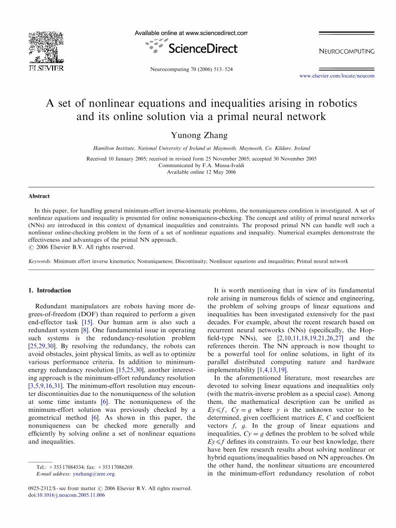
Example 3. Computer simulations are first performedbased on the four-link planar robot [6]. As shown inFig. 4, the manipulator end-point is desired to move alonga circular path initiated from the joint state, yð0Þ ¼ ½3p=4;�p=2;p=4; 0�T rad. The task duration T ¼ 10 s. By solvingthe minimum-effort inverse-kinematic problem, we haveFig. 5 showing the relationship between the discontinuityand nonuniqueness of the minimum-effort solution. They

U (

y)

time (sec)

0 0.002 0.004 0.006 0.008 0.010

0.05

0.1

0.15

0.2

0.25

0.3

0.35

0.4

Fig. 3. Transients of network (13) under the solution existence of (11

-4 -3 -2 -1 0 1 2 3 4-4

-3

-2

-1

0

1

2

3

4

X

Y

0-2

-1

0

1

2

3

4

5

6

7

Fig. 4. Motion trajectories of a four-link planar robot sy

coincide quite well in this example (m ¼ 2 and n ¼ 4). Asshown in Fig. 5(a), the second–fourth joint velocities havediscontinuities during the time periods [3.0, 6.1] and [6.6,9.75] in seconds. As shown in Fig. 5(b), there are extranonuniqueness time-periods near the aforementioned oneslike [2.7, 3.0], [6.1, 6.25] and [9.75, 9.97] in seconds whereUðyÞ ¼ 0. This confirms the results in [6] very well that thenonuniqueness of solution x� to (5)–(8) is a necessarycondition to the discontinuity phenomenon of minimum-effort solutions.

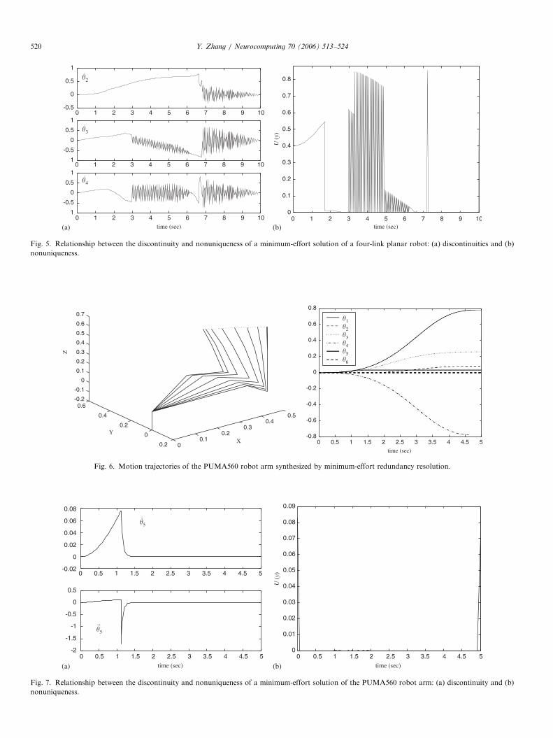
Example 4. Computer simulations of using primal NN (13)are then performed based on the 6DOF UnimationPUMA560 robot arm [25,28] where n ¼ 6 and m ¼ 3. Asshown in Fig. 6, the initial joint state is yð0Þ ¼½0; 0; 0; 0; 0; 0�T rad, and the desired end-effector Cartesianpath is a straight-line trajectory of length 0:2

ffiffiffi2p

m withtask duration T ¼ 5 s. Fig. 7(a) shows that there is only one

time (sec)

0 0.004 0.008 0.012 0.016 0.02-0.8

-0.6

-0.4

-0.2

0

0.2

0.4

0.6

0.8

y5

y4

y2

y3

y1

) with n ¼ 4 and m ¼ 2, starting from arbitrary initial conditions.

1 2 3 4 5 6 7 8 9 10

time (sec)

�1

�2

�3

�4

nthesized by minimum-effort redundancy resolution.

ARTICLE IN PRESS

0 1 2 3 4 5 6 7 8 9 10-0.5

0

0.5

1

0 1 2 3 4 5 6 7 8 9 101

-0.5

0

0.5

1

0 1 2 3 4 5 6 7 8 9 101

-0.5

0

0.5

1

time (sec) time (sec)0 1 2 3 4 5 6 7 8 9 10

0

0.1

0.2

0.3

0.4

0.5

0.6

0.7

0.8

U (

y)

�4

�3

�2

.

.

.

(a) (b)

Fig. 5. Relationship between the discontinuity and nonuniqueness of a minimum-effort solution of a four-link planar robot: (a) discontinuities and (b)

nonuniqueness.

00.1

0.20.3

0.40.5

0.2

0

0.2

0.4

0.6-0.2

-0.1

0

0.1

0.2

0.3

0.4

0.5

0.6

0.7

X

Y

Z

0 0.5 1 1.5 2 2.5 3 3.5 4 4.5 5-0.8

-0.6

-0.4

-0.2

0

0.2

0.4

0.6

0.8

time (sec)

�1�2�3�4�5�6

Fig. 6. Motion trajectories of the PUMA560 robot arm synthesized by minimum-effort redundancy resolution.

0 0.5 1 1.5 2 2.5 3 3.5 4 4.5 5-0.02

0

0.02

0.04

0.06

0.08

0 0.5 1 1.5 2 2.5 3 3.5 4 4.5 5-2

-1.5

-1

-0.5

0

0.5

time (sec) time (sec)

0 0.5 1 1.5 2 2.5 3 3.5 4 4.5 50

0.01

0.02

0.03

0.04

0.05

0.06

0.07

0.08

0.09

�5

�5

.

..

U (

y)

(a) (b)

Fig. 7. Relationship between the discontinuity and nonuniqueness of a minimum-effort solution of the PUMA560 robot arm: (a) discontinuity and (b)

nonuniqueness.

Y. Zhang / Neurocomputing 70 (2006) 513–524520

ARTICLE IN PRESSY. Zhang / Neurocomputing 70 (2006) 513–524 521

discontinuity point that exists in the fifth joint at timeinstant t ¼ 1:1187 s. In contrast, as shown in Fig. 7(b),during almost all the task duration, the minimum-effortsolution is not unique in view of UðyÞ being 0. This impliesthat the nonuniqueness is only a necessary condition to thediscontinuity phenomenon of minimum-effort redundancyresolution.

Example 5. The 7DOF Mitsubishi PA10 robot arm isfinally simulated [31]. The initial state of the robot arm isyð0Þ ¼ ½0;�p=4; 0;p=2; 0;�p=4; 0�T rad and the desired end-effector Cartesian path is a circular trajectory. Thesimulation is shown in Fig. 8. The comparison betweentime periods of nonuniqeness and discontinuity is given inFig. 9. In this PA10 manipulator (n ¼ 7 and m ¼ 3),corresponding to the discontinuity time periods, theadditional nonuniqueness time periods are [3.5, 4.7], [4.8,6.75] and [6.95, 9.5] s, covering almost 90% of the taskduration. This example, together with Example 4, sub-

-0.4-0.3

-0.2-0.1

0

-0.4-0.3

-0.2-0.1

00.1

0.20.3

-0.4

-0.2

0

0.2

0.4

0.6

0.8

1

X

Y

Z

Fig. 8. Motion trajectories of the PA10 robot arm synt

0 1 2 3 4 5 6 7 8 9 10-0.2

-0.1

0

0.1

0.2

0 1 2 3 4 5 6 7 8 9 10-0.2

0

0.2

0.4

0.6

0 1 2 3 4 5 6 7 8 9 10-0.4

-0.2

0

0.2

0.4

time (sec)

U (

y)

�3

.

�5

.

�6

.

(a) (b

Fig. 9. Relationship between the discontinuity and nonuniqueness of a minim

and (b) nonuniqueness.

stantiates that the nonuniqueness points of mini-mum-effort solutions usually exist in high-DOF manip-ulators, which may or may not cause the solutiondiscontinuities. The following analysis might explain whynonuniqueness time periods appear more frequently overthe increase of n. Since C is usually of rank m and y is ofdimension nþ 1, the only zero solution of Eyp0 and Cy ¼

0 lies in

E!

F

�F

~E

264

375; F 2 Rðnþ1�mÞ�ðnþ1Þ; rank

C

F

� �� �¼ nþ 1.

That is, to find matrix F of rank nþ 1�m from E via rowsswap, of which the row vectors together with C rows spanthe Rnþ1 space. As E contains 4nþ 3 rows at most, simplysaying, it is empirically more probable to find nþ 1�m

basis rows from 4nþ 3 rows as the manipulator DOF, n,increases (also refer to Example 2).

0.1

0 1 2 3 4 5 6 7 8 9 10-1.5

-1

-0.5

0

0.5

1

1.5

2

time (sec)

�1

�2

�3

�4

�5

�6

�7

hesized by minimum-effort redundancy resolution.

time (sec)0 1 2 3 4 5 6 7 8 9 10

0

0.1

0.2

0.3

0.4

0.5

0.6

0.7

0.8

)

um-effort solution of the PA10 industrial manipulator: (a) discontinuities

ARTICLE IN PRESS

0 2 4 6 8 102

3

4

5

6

7

8

9

10

11

time (sec)

0 0.5 1 1.5 2 2.5 3 3.5 4 4.5 5

4

6

8

10

12

14

16N

o. o

f E

row

s

No.

of

E r

ows

No.

of

E r

ows

time (sec) time (sec)

0 2 4 6 8 10

2

4

6

8

10

12

14

16

(a) (b) (c)

Fig. 10. The numbers of E rows are time-varying in the robotic context: (a) planar robot, (b) PUMA560 and (c) PA10.

Y. Zhang / Neurocomputing 70 (2006) 513–524522

Remark 5. The above observations generalize the roboticresearch results [6] to the high-DOF situation. It followsfrom our numerical experiments and analysis that,nonuniqueness is a necessary (not sufficient) condition tothe discontinuities of minimum-effort inverse-kinematicsolutions, and that when the minimum-effort redundancyresolution jumps from one solution set to another, thediscontinuity may happen. This could also refer to Fig. 1and the explaining paragraph in Section 2.1. As shown inExample 3, the nonuniqueness is nearly sufficient formanipulators with low degree-of-redundancy, thus able toremedy discontinuities effectively in [6,31]. For manipula-tors with high degree-of-redundancy, other weightingschemes like [5] might be used.

Remark 6. Moreover, as shown in Fig. 10, the numbers ofrows of matrix E are time-varying: sometimes 426 andsometimes more than 10. If nonprimal NNs are used in thiscontext, 4nþ 3 auxiliary neurons are required for handlingE. In comparison, only nþ 1 neurons are used in theproposed primal NN approach. In addition to thecomputational efficiency, this shows another advantageof using primal NNs, especially in the situation of dynamicconstraints and inequalities.

5. Concluding remarks

Minimum-effort solutions could complement the re-search on redundancy resolution in terms of low individualmagnitude, even distribution of workload, and analyzingmotion diversity. In this paper, for investigating theproblem of discontinuities/nonuniqueness appearing inminimum-effort solutions, a set of nonlinear equationsand inequalities has been formulated as a nonuniquenesscriterion. Due to the real-time computation requirement, aprimal NN has been developed to solve online thisminimum-effort nonuniqueness problem. Numerical ex-amples have substantiated the effectiveness and advantagesof the proposed primal-NN computing scheme.

The observations drawn from Examples 3–5 haveprovided new insights and answers to the related

solution-discontinuity problems [3,6,9,16,31]. For example,in minimum-effort redundancy resolution, the relationshipbetween nonuniqueness and discontinuities could besummarized as follows. In the manipulators with lowDOF/redundancy, the nonuniqueness could be a necessaryand nearly sufficient condition to the appearance ofdiscontinuities. In the manipulators with high DOF/redundancy, nonuniqueness could only be a necessarycondition to the discontinuities.

Acknowledgements

The author would like to thank the editors and theanonymous reviewers for their time and effort in providingmany constructive comments. Here, the gratitude isexpressed to them, especially considering that I was makingrevisions around Thanksgiving day.

Appendix A

Proof of Lemma 3. With Ei denoting the ith row of matrixE, we have

kmaxðEy� f ; 0Þk22

¼ maxðEy� f ; 0ÞT maxðEy� f ; 0Þ

¼

maxðE1y� f 1; 0Þ

maxðE2y� f 2; 0Þ

� � �

maxðEiy� f i; 0Þ

� � �

2666666664

3777777775

TmaxðE1y� f 1; 0Þ

maxðE2y� f 2; 0Þ

� � �

maxðEiy� f i; 0Þ

� � �

2666666664

3777777775

¼ maxðE1y� f 1; 0Þ2þmaxðE2y� f 2; 0Þ

2

þ � � � þmaxðEiy� f i; 0Þ2þ � � �

¼XdimðEÞi¼1

maxðEiy� f i; 0Þ2. ð17Þ

ARTICLE IN PRESSY. Zhang / Neurocomputing 70 (2006) 513–524 523

For yj (i.e., the jth element of y), if Eiy� f i40, we have

qmaxðEiy� f i; 0Þ2

qyj

¼qðEiy� f iÞ

2

qyj

¼ 2ðEiy� f iÞqðEiy� f iÞ

qyj

¼ 2ðEiy� f iÞEij

¼ 2maxðEiy� f i; 0ÞEij. ð18Þ

The above result is also achievable in the case of Eiy� f ip0:

qmaxðEiy� f i; 0Þ2

qyj

¼q0qyj

¼ 0 ¼ 2maxðEiy� f i; 0ÞEij , (19)

which is in view of maxðEiy� f i; 0Þ ¼ 0 as Eiy� f ip0.Thus, no matter whether Eiy� f i40 or not, it follows from(17), (18) and (19) that

qkmaxðEy� f ; 0Þk22qyj

¼qP

maxðEiy� f i; 0Þ2

qyj

¼ 2XdimðEÞi¼1

maxðEiy� f i; 0ÞEij.

Now, we have the derivative of kmaxðEy� f ; 0Þk22 withrespect to y as

dkmaxðEy� f ; 0Þk22dy

¼

qkmaxðEy� f ; 0Þk22=qy1

qkmaxðEy� f ; 0Þk22=qy2

� � �

qkmaxðEy� f ; 0Þk22=qyj

� � �

2666666664

3777777775

¼

2PdimðEÞi¼1

maxðEiy� f i; 0ÞEi1

2PdimðEÞi¼1

maxðEiy� f i; 0ÞEi2

� � �

2PdimðEÞi¼1

maxðEiy� f i; 0ÞEij

� � �

266666666666664

377777777777775,

which equals the following matrix form

2ET maxðEy� f ; 0Þ

¼ 2

E11 E21 � � � Ei1 � � �

E12 E22 � � � Ei2 � � �

� � � � � � � � � � � � � � �

E1j E2j � � � Eij � � �

� � � � � � � � � � � � � � �

2666666664

3777777775

maxðE1y� f 1; 0Þ

maxðE2y� f 2; 0Þ

� � �

maxðEiy� f i; 0Þ

� � �

2666666664

3777777775.

The proof is thus completed. &

Appendix B

Proof of Lemma 4. For yj (the jth element of y), we couldderive that

qðyTy� hÞ2=2

qyj

¼ ðyTy� hÞqðyTy� hÞ

qyj

¼ ðyTy� hÞ2yj .

According to the definition of the derivative of a scalarfunction with respect to a vector, we thus have

dðyTy� hÞ2=2

dy¼

qðyTy� hÞ2=2

qy1

qðyTy� hÞ2=2

qy2

� � �

qðyTy� hÞ2=2

qyj

� � �

266666666666664

377777777777775¼

ðyTy� hÞ2y1

ðyTy� hÞ2y2

� � �

ðyTy� hÞ2yj

� � �

2666666664

3777777775

¼ 2ðyTy� hÞy,

which completes the proof. &

References

[1] N.M. Botros, M. Abdul-Aziz, Hardware implementation of an

artificial neural network using field programmable gate arrays

(FPGAs), IEEE Trans. Ind. Electron. 41 (6) (1994) 665–667.

[2] A. Cichocki, R. Unbehauen, Neural networks for solving systems of

linear equation and related problems, IEEE Trans. Circuits Syst. I 39

(2) (1992) 124–138.

[3] A.S. Deo, I.D. Walker, Minimum effort inverse kinematics for

redundant manipulators, IEEE Trans. Robotics Autom. 13 (5) (1997)

767–775.

[4] C. Diorio, R.P.N. Rao, Neural circuits in silicon, Nature 405 (6789)

(2000) 891–892.

[5] S.S. Ge, Y. Zhang, T.H. Lee, An acceleration-based weighting

scheme for minimum-effort inverse kinematics of redundant manip-

ulators, Proceedings of the IEEE International Symposium on

Intelligent Control, 2004, pp. 275–280.

[6] I.A. Gravagne, I.D. Walker, On the structure of minimum effort

solutions with application to kinematic redundancy resolution, IEEE

Trans. Robotics Autom. 16 (6) (2000) 855–863.

[7] K. Iqbal, Y.C. Pai, Predicted region of stability for balance recovery:

motion at the knee joint can improve termination of forward

movement, J. Biomechanics 33 (12) (2000) 1619–1627.

[8] M.L. Latash, Control of Human Movement, Human Kinetics

Publisher, Chicago, 1993.

[9] J. Lee, A structured algorithm for minimum l1-norm solutions and

its application to a robot velocity workspace analysis, Robotica 19 (3)

(2001) 343–352.

[10] X. Liang, S.K. Tso, An improved upper bound on step-size

parameters of discrete-time recurrent neural networks for linear

inequality and equation system, IEEE Trans. Circuits Syst. 49 (5)

(2002) 695–698.

[11] F.L. Luo, B. Zheng, Neural network approach to computing matrix

inversion, Appl. Math. Comput. 47 (2–3) (1992) 109–120.

[12] O.L. Mangasarian, Uniqueness of solution in linear programming,

Linear Algebra Appl. 25 (1979) 151–162.

[13] C. Mead, Analog VLSI and Neural Systems, Addison-Wesley,

Reading, MA, 1989.

[14] R. Saigal, Linear Programming: a Modern Integrated Analysis,

Kluwer Academic Publishers, Norwell, MA, 1995.

ARTICLE IN PRESSY. Zhang / Neurocomputing 70 (2006) 513–524524

[15] L. Sciavicco, B. Siciliano, Modelling and Control of Robot

Manipulators, Springer-Verlag, London, 2000.

[16] I.-C. Shim, Y.-S. Yoon, Stabilized minimum infinity-norm torque for

redundant manipulators, Robotica 16 (1998) 193–205.

[17] J.-J.E. Slotine, W. Li, Applied Nonlinear Control, Prentice-Hall,

Englewood Cliffs, NJ, 1991.

[18] J. Song, Y. Yam, Complex recurrent neural network for computing

the inverse and pseudo-inverse of the complex matrix, Appl. Math.

Comput. 93 (2–3) (1998) 195–205.

[19] D.W. Tank, J.J. Hopfield, Simple neural optimization networks: an

A/D converter, signal decision circuit, and a linear programming

circuit, IEEE Trans. Circuits Syst. 33 (1986) 533–541.

[20] J. Wang, Y. Zhang, Recurrent neural networks for real-time

computation of inverse kinematics of redundant manipulators, in:

Machine Intelligence: Quo Vadis?, World Scientific, Singapore, 2004.

[21] L.-X. Wang, J.M. Mendel, Three-dimensional structured network for

matrix equation solving, IEEE Trans. Comput. 40 (12) (1991)

1337–1345.

[22] S. Zhang, A.G. Constantinides, Lagrange programming neural

networks, IEEE Trans. Circuits Syst. 39 (7) (1992) 441–452.

[23] X. Zhang, D.B. Chaffin, An inter-segment allocation strategy for

postural control in human reach motions revealed by differential

inverse kinematics and optimization, Proceedings of IEEE Interna-

tional Conference on Systems, Man, and Cybernetics, 1997,

pp. 469–474.

[25] Y. Zhang, S.S. Ge, T.H. Lee, A unified quadratic programming based

dynamical system approach to joint torque optimization of physically

constrained redundant manipulators, IEEE Trans. Syst. Man

Cybern. Part B 34 (5) (2004) 2126–2132.

[26] Y. Zhang, D. Jiang, J. Wang, A recurrent neural network for solving

Sylvester equation with time-varying coefficients, IEEE Trans.

Neural Networks 13 (5) (2002) 1053–1063.

[27] Y. Zhang, J. Wang, Global exponential stability of recurrent

neural networks for synthesizing linear feedback control systems

via pole assignment, IEEE Trans. Neural Networks 13 (3) (2002)

633–644.

[28] Y. Zhang, J. Wang, A dual neural network for constrained joint

torque optimization of kinematically redundant manipulators, IEEE

Trans. Syst. Man Cybern. 32 (5) (2002) 654–662.

[29] Y. Zhang, J. Wang, Obstacle avoidance for kinematically redundant

manipulators using a dual neural network, IEEE Trans. Syst. Man

Cybern. Part B 34 (1) (2004) 752–759.

[30] Y. Zhang, J. Wang, Y. Xia, A dual neural network for redundancy

resolution of kinematically redundant manipulators subject to joint

limits and joint velocity limits, IEEE Trans. Neural Networks 14 (3)

(2003) 658–667.

[31] Y. Zhang, J. Wang, Y. Xu, A dual neural network for bi-criteria

kinematic control of redundant manipulators, IEEE Trans. Robotics

Autom. 18 (6) (2002) 923–931.

Yunong Zhang was born in Xinyang, Henan, PR

China in October 1973. He received the B.E.

degree from the Huazhong University of Science

and Technology (HUST) in 1996, the M.E.

degree from the South China University of

Technology (SCUT) in 1999. He completed his

Ph.D. study in the Chinese University of Hong

Kong (CUHK) in November 2002 with the

degree received in 2003. Then, as a research

fellow he had been with the National University

of Singapore (NUS), and the University of Strathclyde, United Kingdom,

respectively, in 2003 and 2004. After that, he has been with the National

University of Ireland, Maynooth (NUIM) as a research scientist. His

current research interests are redundant robot manipulators and the

related biomechanics research, recurrent neural networks and their

hardware/circuits implementation, and scientific computing and optimiza-

tion such as Gaussian process regression.