A Regression-based Adjusted Plus-MinusStatistic for NHL Players

Brian Macdonald

May 29, 2018

Abstract

The goal of this paper is to develop an adjusted plus-minus statistic forNHL players that is independent of both teammates and opponents. We usedata from the shift reports on NHL.com in a weighted least squares regres-sion to estimate an NHL player’s effect on his team’s success in scoring andpreventing goals at even strength. Both offensive and defensive componentsof adjusted plus-minus are given, estimates in terms of goals per 60 minutesand goals per season are given, and estimates for forwards, defensemen, andgoalies are given.

Keywords: plus-minus, hockey, nhl, sports

1

arX

iv:1

006.

4310

v3 [

stat

.AP]

1 N

ov 2

010

Contents1 Introduction 4

1.1 Example of the Results . . . . . . . . . . . . . . . . . . . . . . . 51.2 Complete Results . . . . . . . . . . . . . . . . . . . . . . . . . . 6

2 Two weighted least-squares models 72.1 Ilardi-Barzilai-type model . . . . . . . . . . . . . . . . . . . . . 72.2 Calculating OPM, DPM, and APM . . . . . . . . . . . . . . . . . 92.3 Rosenbaum-type model . . . . . . . . . . . . . . . . . . . . . . . 102.4 Averaging results from the two models . . . . . . . . . . . . . . . 12

3 Summary of Results 123.1 OPM/60 . . . . . . . . . . . . . . . . . . . . . . . . . . . . . . 133.2 OPM . . . . . . . . . . . . . . . . . . . . . . . . . . . . . . . . 153.3 DPM/60 . . . . . . . . . . . . . . . . . . . . . . . . . . . . . . 163.4 DPM . . . . . . . . . . . . . . . . . . . . . . . . . . . . . . . . 213.5 APM/60 . . . . . . . . . . . . . . . . . . . . . . . . . . . . . . . 243.6 APM . . . . . . . . . . . . . . . . . . . . . . . . . . . . . . . . . 27

4 Discussion of the Model 294.1 Advantages of APM . . . . . . . . . . . . . . . . . . . . . . . . . 304.2 Disadvantages of APM . . . . . . . . . . . . . . . . . . . . . . . 314.3 Selection of the variables . . . . . . . . . . . . . . . . . . . . . . 314.4 Selection of the observations . . . . . . . . . . . . . . . . . . . . 324.5 Discussion of assumptions . . . . . . . . . . . . . . . . . . . . . 32

4.5.1 Goalie contribution on offense . . . . . . . . . . . . . . . 334.5.2 Interactions between players . . . . . . . . . . . . . . . . 34

4.6 Discussion of Errors . . . . . . . . . . . . . . . . . . . . . . . . 344.7 Future work and conclusions . . . . . . . . . . . . . . . . . . . . 37

2

List of Tables1.1.1 Top 10 Players in OPM . . . . . . . . . . . . . . . . . . . . . . . 51.2.1 Example of Linemate Details . . . . . . . . . . . . . . . . . . . . 61.2.2 Example of GF, GA, and NG statistics . . . . . . . . . . . . . . . 73.1.1 Top 10 Players in OPM60 . . . . . . . . . . . . . . . . . . . . . 133.1.2 Top 10 Defensemen in OPM60 (minimum 700 minutes) . . . . . 143.2.1 Top 10 Defensemen in OPM . . . . . . . . . . . . . . . . . . . . 153.3.1 Top 10 Players in DPM60 . . . . . . . . . . . . . . . . . . . . . 163.3.2 Top 10 Players in DPM60 (minimum 700 minutes) . . . . . . . . 173.3.3 Top 10 Skaters in DPM60 (minimum 700 minutes) . . . . . . . . 183.3.4 Top 10 Forwards in DPM60 (minimum 700 minutes) . . . . . . . 193.3.5 Top 10 Defensemen in DPM60 (minimum 700 minutes) . . . . . 193.3.6 Top 10 Goalies in DPM60 (minimum 700 minutes) . . . . . . . . 203.4.1 Top 10 Players in DPM . . . . . . . . . . . . . . . . . . . . . . . 223.4.2 Top 10 Skaters in DPM . . . . . . . . . . . . . . . . . . . . . . . 223.4.3 Top 10 Forwards in DPM . . . . . . . . . . . . . . . . . . . . . 233.4.4 Top 10 Defensemen in DPM . . . . . . . . . . . . . . . . . . . . 243.5.1 Top 10 Players in APM60 (minimum 700 minutes) . . . . . . . . 253.5.2 Top 10 Forwards in APM60 (minimum 700 minutes) . . . . . . . 263.5.3 Top 10 Defensemen in APM60 (minimum 700 minutes) . . . . . 263.6.1 Top 10 Players in APM . . . . . . . . . . . . . . . . . . . . . . . 283.6.2 Top 10 Skaters in APM . . . . . . . . . . . . . . . . . . . . . . . 283.6.3 Top 10 Defensemen in APM . . . . . . . . . . . . . . . . . . . . 294.6.1 Top 10 Players in Highest Err in APM60 (minimum 700 minutes) 354.6.2 Top 10 Players in Lowest Err in APM60 (minimum 700 minutes) 364.6.3 Top 10 Skaters in Lowest Err in APM60 (minimum 700 minutes) 36

List of Figures3.1.1 Kernel Density Estimation for OPM/60 and OPM . . . . . . . . . 143.3.1 Kernel Density Estimation for DPM/60 and DPM . . . . . . . . . 173.5.1 Kernel Density Estimation for APM/60 and APM . . . . . . . . . 254.6.1 Kernel Density Estimation for APM/60 Errors and APM Errors. . 37

3

1 IntroductionHockey analysts have developed several metrics that attempt to quantify an NHLplayer’s contribution to his team. Tom Awad’s Goals Versus Threshold in Awad(2009), Jim Corsi’s Corsi rating as described in Boersma (2007), Gabriel Des-jardins’ Behindthenet Rating, along with his on-ice/off-ice, strength of opponents,and strength of linemates statistics in Desjardins (2010), Iian Fyffe’s Point Al-location in Fyffe (2002), Ken Krzywicki’s shot quality, as presented in Krzy-wicki (2005) and updated in Krzywicki (2009), Alan Ryder’s Player Contribu-tion in Ryder (2004), and Timo Seppa’s Even-Strength Total Rating in Seppa(2009) are a few examples. In this paper, we propose a new metric, adjustedplus-minus (APM), that attempts to estimate a player’s contribution to his team ineven-strength (5-on-5, 4-on-4, and 3-on-3) situations, independent of that player’steammates and opponents, and in the units of goals per season. APM can also beexpressed in terms of goals per 60 minutes (APM/60). We find both an adjustedoffensive plus-minus component (OPM) and an adjusted defensive plus-minuscomponent (DPM), which estimate the offensive and defensive production of aplayer at even-strength, independent of teammates and opponents, and in the unitsof goals per season.

Inspired by the work in basketball by Rosenbaum (2004), Ilardi and Barzilai(2008), and Witus (2008), we use weighted multiple linear regression models toestimate OPM per 60 minutes (OPM/60) and DPM per 60 minutes (DPM/60).The estimates are a measure of the offensive and defensive production of a playerin the units of goals per 60 minutes. These statistics, along with average minutesplayed per season, give us OPM and DPM. Adding OPM/60 and DPM/60 givesAPM/60, and adding OPM and DPM gives APM. We emphasize that we consideronly even-strength situations.

The main benefit of the weighted linear regression model is that the resultingadjusted plus-minus statistics for each player should in theory be independentof that player’s teammates and opponents. The traditional plus-minus statistic inhockey is highly dependent on a player’s teammates and opponents, and the use ofthe regression removes this dependence. One drawback of our model is statisticalnoise. In order to improve the estimates and reduce the standard errors in theestimates, we use data from three NHL seasons, and we combine the results oftwo different models, one inspired by Ilardi and Barzilai (2008), and the other byRosenbaum (2004).

4

1.1 Example of the ResultsBefore we describe the models in detail, we give the reader an example of theresults. The typical NHL fan has some idea of who the best offensive players inthe league are, so we give the top 10 players in average OPM during the 2007-08, 2008-09, and 2009-10 seasons, sorted by OPM, in Table 1.1.1. Note that Rk

Table 1.1.1: Top 10 Players in OPM

Rk Player Pos OPM OErr DPM APM Mins GF60 OPM60 GF

1 Pavel Datsyuk C 15.4 3.4 6.2 21.6 1186 3.39 0.777 672 Alex Ovechkin LW 15.2 3.8 0.2 15.4 1262 3.69 0.723 783 Sidney Crosby C 14.4 2.6 −0.9 13.5 1059 3.59 0.818 634 Henrik Sedin C 14.0 4.5 −5.7 8.3 1169 3.35 0.718 655 Evgeni Malkin C 13.2 2.7 −3.0 10.2 1164 3.37 0.681 656 Zach Parise LW 12.6 3.2 3.0 15.6 1164 2.94 0.652 577 Joe Thornton C 12.0 3.2 3.6 15.6 1222 3.13 0.590 648 Eric Staal C 11.5 3.1 −0.5 11.0 1159 3.00 0.594 589 Ilya Kovalchuk LW 10.9 2.8 −4.2 6.7 1189 2.93 0.551 5810 Marian Gaborik RW 10.2 2.2 4.3 14.5 853 3.28 0.715 47

is the rank of that player in terms of OPM, Pos is the player’s position, OErris the standard error in the OPM estimates, Mins is the number of minutes thatthe player played on average during the 2007-08, 2008-09, and 2009-10 seasons,GF60 are the goals per 60 minutes that a player’s team scored while he was theice at even-strength, and GF are the goals per season that a player’s team scoredwhile he was the ice at even-strength. The 10 players in this list are arguablythe best offensive players in the game. Ovechkin, Crosby, Datsyuk, and Malkin,perhaps the league’s most recognizable superstars, make the top 5 along withHenrik Sedin, who led the NHL in even-strength points during the 2009-2010season with 83 points, which was 10 more points than the next leading scorer.

We highlight two interesting numbers in this list. First, note that Pavel Dat-syuk, who is regarded by many as the best two-way player in the game, has thehighest defensive rating among these top offensive players. Datsyuk’s excellenttwo-way play gives him the highest APM estimate among forwards and defense-men. We give the list of top 10 forwards and defensemen in APM, and discussseveral other top 10 lists for OPM/60,OPM,DPM/60,DPM,APM/60, and APM,in Section 3. Second, note that Henrik Sedin has a much higher OErr than the

5

other players in the list. This increased error is likely due to the fact that Henrikplays most of his minutes with his brother Daniel, and the model has a difficulttime separating the contributions of the twin brothers. The Sedin twins provide uswith a great example to use when analyzing the errors, and we discuss the Sedinsand the errors in more detail in Section 4.6.

1.2 Complete ResultsA .csv file containing the complete results can be obtained by contacting theauthor. An interested reader may prefer to open these results in a spreadsheetprogram and filter by position or sort by a particular statistic. Also, the .csv filecontains more columns than the list given in Table 1.1.1. For example, the file in-cludes the three most frequent linemates of each player along with the percentageof minutes played with each of those linemates during the 2007-08, 2008-09, and2009-10 NHL regular seasons. An example of these additional columns is givenin Table 1.2.1. Notice that, as suggested in the table, Henrik Sedin played 83%

Table 1.2.1: Example of Linemate Details

Player Pos Mins Teammate.1 min1 Teammate.2 min2 Teammate.3 min3

Henrik Sedin C 1169 D.Sedin 83% R.Luongo 76% A.Edler 35%Daniel Sedin LW 1057 H.Sedin 92% R.Luongo 77% A.Edler 35%

of his minutes with brother Daniel, and Daniel played 92% of his minutes withHenrik.

Finally, the file includes columns for the goals a player’s team scored (GF),the goals a player’s team allowed (GA), and the net goals a player’s team scored(NG), while he was on the ice at even-strength. These statistics are in terms ofaverage goals per season during the 2007-08, 2008-09, and 2009-10 NHL regularseasons. We also give GF/60,GA/60, and NG/60, which are GF,GA, and NG interms of goals per 60 minutes. An example of this information is given in Table1.2.2. These raw statistics, along with the linemate information, will be helpful inthe analysis of the results of our model.

The rest of this paper is organized as follows. In Section 2, we describe thetwo models we use to compute OPM, DPM, and APM. In Section 3, we summa-rize and discuss the results of these models by giving various top 10 lists, indi-cating the best forwards, defensemen, and goalies according to OPM, DPM, and

6

Table 1.2.2: Example of GF, GA, and NG statistics

Player Pos GF60 GA60 NG60 GF GA NG

Sidney Crosby C 3.59 2.55 1.04 63 45 18Pavel Datsyuk C 3.39 1.84 1.55 67 36 31

APM, as well as their corresponding per 60 minute statistics. Section 4 containsa discussion of the model. We summarize and discuss the advantages (4.1) anddisadvantages (4.2) of these statistics. Next, we give more details about the for-mation of the model, including the selection of the variables (4.3), and selectionof the observations (4.4). Also, we discuss our assumptions (4.5) as well as thestandard errors (4.6) in the estimates. We finish with ideas for future work andsome conclusions (4.7).

2 Two weighted least-squares modelsWe now define our variables and state our models. In each model, we use playerswho have played a minimum of 4000 shifts over the course of the 2007-08, 2008-09, and 2009-10 seasons (see Section 4 for a discussion). We define a shift to be aperiod of time during the game when no substitutions are made. The observationsin each model are weighted by the duration of that observation in seconds.

2.1 Ilardi-Barzilai-type modelInspired by Ilardi and Barzilai (2008), we use the following linear model:

y = β0 +β1X1 + · · ·+βJXJ +δ1D1 + · · ·+δJDJ + γ1G1 + · · ·+ γKGK + ε, (1)

7

where J is the number of skaters in the league, and K is the number of goalies inthe league. The variables in the model are defined as follows:

y = goals per 60 minutes during an observation

X j =

{1, skater j is on offense during the observation;0, skater j is not playing or is on defense during the observation;

D j =

{1, skater j is on defense during the observation;0, skater j is not playing or is on offense during the observation;

Gk =

{1, goalie k is on defense during the observation;0, goalie k is not playing or is on offense during the observation;

where 1 ≤ j ≤ J, and 1 ≤ k ≤ K. Note that by “skater” we mean a forward or adefensemen, but not a goalie. The coefficients in the model have the followinginterpretation:

β j = goals per 60 minutes contributed by skater j on offense,−δ j = goals per 60 minutes contributed by skater j on defense,−γk = goals per 60 minutes contributed by goalie k on defense, (2)

β0 = intercept,ε = error.

The coefficient β1, for example, gives an estimate, in goals per 60 minutes, ofhow y changes when Skater 1 is on the ice on offense (X1 = 1) versus when Skater1 is not on the ice on offense (X1 = 0), independent of all other players on theice. The coefficients β j,−δ j, and −γk are estimates of OPM/60 for Skater j,DPM/60 for Skater j, and DPM/60 for Goalie k, respectively. They are playing-time-independent rate statistics, measuring the offensive and defensive value of aplayer in goals per 60 minutes.

Notice the negative sign in front of δ j and γk in (2). Note that a negative valuefor one of these coefficients corresponds to a positive contribution. For example,if Skater 1 has a defensive coefficient of δ1 = −0.8, he prevents 0.8 goals per60 minutes when he is on defense. We could have chosen to define a skater’sDPM/60 to be +δ j, in which case negative values for DPM/60 would be good.Instead, we prefer that positive contributions be represented by a positive number,so we define DPM/60 = −δ j for skaters. Likewise, we define DPM/60 = −γkfor goalies. For Skater 1’s DPM/60 in our example, we have

DPM/60 =−δ1 =−(−0.8) = +0.8,

8

which means that Player 1 has a positive contribution of +0.8 goals per 60 minuteson defense.

Note that for the observations in this model, each shift is split into two lines ofdata: one line corresponding to the home team being on offense, and one line cor-responding to the away team being on offense. It is assumed that in hockey, unlikein other sports, a team plays offense and defense concurrently, and the two obser-vations for each shift are given equal weight. Also, note that we include separatedefensive variables for goalies, but no offensive variables. Here we are assumingthat goalies do not contribute on offense. See Section 4.5 for a discussion of theseassumptions. Finally, we note that the data used for the model were obtained fromthe shift charts published in NHL.com (2010) for games played in the 2007-08,2008-09, and 2009-10 regular seasons. See Section 4.4 for more about the dataused and to see how it was selected.

2.2 Calculating OPM, DPM, and APM

A player’s contribution in terms of goals over an entire season is useful as well,and may be preferred by some NHL fans and analysts. We use the regressioncoefficients and minutes played to give playing-time-dependent counting statisticversions of the rate statistics from the regression model. These counting statisticsare OPM, DPM, and APM, and they measure the offensive, defensive, and totalvalue of a player, in goals per season. To get a skater’s OPM, for example, wemultiply a skater’s offensive contribution per minute by the average number ofminutes that the skater played per season from 2007-2010. The value for DPMis found likewise, and APM for a player is the sum of his OPM and his DPM.Goalies have no OPM, so a goalie’s APM is simply his DPM. Let

MinO j = minutes per season on offense for skater j,MinD j = minutes per season on defense for skater j, andMinGk = minutes per season on defense for goalie k.

Then, we can calculate OPM,DPM, and APM for skaters and goalies as follows:

OPM j = β j MinO j/60,DPM j =−δ j MinD j/60 (for skaters),DPMk =−γk MinGk/60 (for goalies), (3)APM j = OPM j +DPM j (for skaters),APMk = DPMk (for goalies).

9

In order to estimate Err, the standard errors for the APM estimates, we assumethat OPM and DPM are uncorrelated, and we have

Err =√

Var(APM) =√

(OErr)2 +(DErr)2.

where OErr and DErr are the standard errors in the OPM and DPM estimates,respectively, and Var is variance. The assumption that offensive and defensivecontributions of a player are uncorrelated is debatable. See, for example, Pronman(2010).

2.3 Rosenbaum-type modelIn an effort to improve the estimates and their errors, we use a second linear model,this one inspired by Rosenbaum (2004):

ynet = η0 +η1N1 + · · ·+ηJ+KNJ+K + ε. (4)

The variables in the model are defined as follows:

ynet = net goals per 60 minutes for the home team during an observation

N j =

1, player j is on the home team during the observation;

−1, player j is on the away team during the observation;0, player j is not playing during the observation.

The coefficients in the model have the following interpretation:

η j = net goals per 60 minutes contributed by player j,η0 = intercept,ε = error.

The coefficients η1, . . . ,ηJ of this model are estimates of each player’s APM/60.By “net goals” we mean the home team’s Goals For (GF) minus the home team’sGoals Against (GA). Also, note that by “player” we mean forward, defensemen, orgoalie. The data used for these variables were also obtained from the shift chartspublished on NHL.com for games played in the 2007-08, 2008-09, and 2009-10regular seasons. In this model, unlike the Ilardi-Barzilai model, each observationin this model is simply one shift. We do not split each shift into two lines of data.

In order to separate offense and defense, we follow Rosenbaum and form asecond model:

ytot = τ0 + τ1T1 + · · ·+ τJ+KTJ+K + ε. (5)

10

The variables in the model are defined as follows:

ytot = total goals per 60 minutes scored by both teams during an observation

Tj =

{1, player j is on the ice (home or away) during the observation;0, player j is not on the ice during the observation.

The coefficients in the model have the following interpretation:

τ j = total goals per 60 minutes contributed by skater j,τ0 = intercept,ε = error.

By total goals, we mean GF +GA. Recall that the coefficients in (4) were esti-mates of each player’s APM/60, or net goals contributed per 60 minutes. Like-wise, the coefficients in (5) are estimates of each player’s T PM/60, or total goalscontributed per 60 minutes. In (3), we used playing time to convert APM/60 toAPM, and likewise, we can convert T PM/60 to T PM.

We know from before that

APM/60 = OPM/60+DPM/60, (6)

and we also have that

T PM/60 = OPM/60−DPM/60. (7)

Using equations (6) and (7), if we add a player’s T PM/60 and APM/60, anddivide by 2, the result is that player’s OPM/60:

12(APM/60+T PM/60) = OPM/60.

Likewise,

12(APM/60−T PM/60) = DPM/60.

Using playing time, we can convert OPM/60, DPM/60, and APM/60 to OPM,DPM, and APM as we did with our first model in Section 2.1. Note that in thismodel, unlike the model in Section 2.1, all players are treated the same, whichmeans that the model gives offensive estimates for goalies and skaters alike. Whilea goalie can impact a team’s offensive production, we typically do not use theseoffensive estimates for goalies. Goalies and offense are discussed more in Section4.5.1.

11

2.4 Averaging results from the two modelsThe estimates obtained from the models in Section 2.1 and 2.3 can be averaged,and the resulting estimates will have smaller standard errors than the individualestimates from either of the two models. Let OPMib

j , DPMibj , and APMib

j be theOPM, DPM, and APM results for player j from the Ilardi-Barzilai-type model(Section 2.1), and likewise let OPMr

j , DPMrj , and APMr

j be the correspondingresults from the Rosenbaum-type model (Section 2.3). We average the resultsfrom our two models to arrive at our final metrics OPM, DPM, and APM:

OPM j =12(OPMib

j +OPMrj),

DPM j =12(DPMib

j +DPMrj),

APM j =12(APMib

j +APMrj).

Each model has its advantages and disadvantages, so we have chosen to weightthe results from the two models equally. See Section 4.5.1 for a discussion of thebenefits and drawbacks of each model. Assuming the errors are uncorrelated wecan estimate them as follows:

OErr j =12

√(OErrib

j )2 +(OErrr

j)2,

DErr j =12

√(DErrib

j )2 +(DErrr

j)2,

Err j =12

√(Errib

j )2 +(Errr

j)2.

Note that the errors OErr j are smaller than the errors OErrrj and OErrib

j . Like-wise, DErr j and Err j are smaller than each of the components used to computethem.

3 Summary of ResultsIn this section we will summarize the results of the model by giving various top10 lists, indicating the best offensive, defensive, and overall players in the leagueaccording to the estimates found in the model.

12

3.1 OPM/60

Recall that OPM/60 is a measure of the offensive contribution of a player at even-strength in terms of goals per 60 minutes of playing time. Recall also that weassume that goalies do not contributed on offense, so we list only forwards anddefensemen in this section. The list of top players in OPM/60 is given in Table

Table 3.1.1: Top 10 Players in OPM60

Rk Player Pos OPM60 OErr DPM60 APM60 Mins GF60 OPM GF

1 Sidney Crosby C 0.818 0.148 −0.052 0.766 1059 3.59 14.4 632 Pavel Datsyuk C 0.777 0.174 0.314 1.091 1186 3.39 15.4 673 Alex Radulov RW 0.758 0.222 −0.248 0.510 343 3.67 4.3 214 Alex Ovechkin LW 0.723 0.178 0.010 0.733 1262 3.69 15.2 785 Henrik Sedin C 0.718 0.231 −0.294 0.424 1169 3.35 14.0 656 Marian Gaborik RW 0.715 0.155 0.303 1.018 853 3.28 10.2 477 Evgeni Malkin C 0.681 0.141 −0.156 0.525 1164 3.37 13.2 658 Zach Parise LW 0.652 0.166 0.155 0.807 1164 2.94 12.6 579 Jakub Voracek RW 0.642 0.186 −0.045 0.597 621 3.03 6.6 3110 C. Gunnarsson D 0.608 0.245 0.233 0.841 240 2.91 2.4 12

3.1.1. The players in this list are are regarded by many as being among the bestoffensive players in the game, with the exception of a few players with low min-utes played and higher errors: Alexander Radulov, Jakub Voracek, and Carl Gun-narsson. Those players have far fewer minutes than the other players, and theirestimates are less reliable. Interestingly, Henrik Sedin actually has the secondhighest standard error in the list, even higher than Radulov and Voracek, despitethe fact that he has much higher minutes played totals. This is likely due to thefact that he spends most of his time playing with his brother Daniel (see Section4.6).

Forwards dominated the list in Table 3.1.1. That forwards are more prevalentthan defensemen on this list is not unexpected, as one would probably assumethat forwards contribute to offense more than defensemen do. We can see thistrend more clearly by plotting the kernel density estimation for OPM/60 for bothforwards and defensemen. This plot gives us an approximation of the histogramof our OPM/60 estimates for forwards and defensemen. See Figure 3.1.1. Thecurve for forwards lies to the right of the curve for defensemen, suggesting that the

13

Figure 3.1.1: Kernel Density Estimation for OPM/60 Estimates and OPM Esti-mates.

−0.5 0.0 0.5 1.0

0.0

0.5

1.0

1.5

2.0

2.5

N = 447 Bandwidth = 0.0546

Den

sity

OPM/60 Estimates

Forwards

Defensemen

−5 0 5 10 15

0.00

0.05

0.10

0.15

0.20

N = 447 Bandwidth = 0.654

Den

sity

OPM Estimates

Forwards

Defensemen

OPM/60 estimates for forwards are generally higher than the OPM/60 estimatesfor defensemen.

Since forwards dominated the list of top players in OPM/60, we give the topdefensemen in OPM/60 in Table 3.1.2. There are some top offensive defensemen

Table 3.1.2: Top 10 Defensemen in OPM60 (minimum 700 minutes)

Rk Player Pos OPM60 OErr DPM60 APM60 Mins GF60 OPM GF

10 C. Gunnarsson D 0.608 0.245 0.233 0.841 240 2.91 2.4 1246 Ville Koistinen D 0.424 0.210 0.082 0.506 380 2.89 2.7 1871 Andrei Markov D 0.370 0.162 0.036 0.405 1114 2.69 6.9 5079 Mike Green D 0.357 0.146 0.195 0.552 1334 3.30 7.9 7382 Mark Streit D 0.353 0.136 −0.060 0.293 1199 2.60 7.1 5295 Johnny Oduya D 0.342 0.143 0.116 0.458 1209 2.78 6.9 56112 S. Robidas D 0.313 0.147 0.115 0.428 1316 2.60 6.9 57113 Ian White D 0.311 0.127 0.028 0.338 1343 2.73 6.9 61119 S. Brookbank D 0.302 0.164 0.163 0.465 640 2.44 3.2 26122 Bret Hedican D 0.297 0.166 −0.162 0.135 594 2.96 2.9 29

14

in this list, along with some players with low minutes, high errors, and skepticalratings. One example is Carl Gunnarsson, who tops this list and is one of theplayers with low minutes. Gunnarsson did have a decent season offensively in2009-10, scoring 12 even-strength points in 43 games, while playing just the 6thmost minutes per game among defensemen on his team. Projecting his statisticsover 82 games, Gunnarsson would have had 23 even-strength points, tying himwith Tomas Kaberle for the team lead among defensemen, despite playing lessminutes. So we do get an idea of why the model gave him this high estimate. Wenote that the lower end of the 95% confidence interval for Gunnarsson’s OPM/60is 0.118, suggesting that, at worst, he was still an above average offensive defense-man at even-strength during the limited minutes that he played.

3.2 OPM

Recall that OPM is a measure of the offensive contribution of a player at even-strength in terms of goals over an entire season. Once again, we list only forwardsand defensemen in this section. The top 10 players in OPM were already givenand discussed in the introduction, Table 1.1.1. That list was dominated by for-wards, a trend that can also be seen in Figure 3.1.1, so we now discuss the top 10defensemen in OPM given in Table 3.2.1. Most of the players in Table 3.2.1 are

Table 3.2.1: Top 10 Defensemen in OPM

Rk Player Pos OPM OErr DPM APM Mins GF60 OPM60 GF

22 Mike Green D 7.9 3.2 4.3 12.3 1334 3.30 0.357 7331 Mark Streit D 7.1 2.7 −1.2 5.9 1199 2.60 0.353 5235 Andrei Markov D 6.9 3.0 0.7 7.5 1114 2.69 0.370 5037 Ian White D 6.9 2.8 0.6 7.6 1343 2.73 0.311 6139 S. Robidas D 6.9 3.2 2.5 9.4 1316 2.60 0.313 5740 Johnny Oduya D 6.9 2.9 2.3 9.2 1209 2.78 0.342 5644 Zdeno Chara D 6.6 3.9 2.2 8.8 1441 2.64 0.276 6348 Dion Phaneuf D 6.4 3.2 −0.7 5.6 1443 2.76 0.265 6653 Duncan Keith D 6.2 4.2 7.3 13.5 1532 2.94 0.245 7567 Dan Boyle D 5.6 2.7 −1.6 4.0 1169 2.69 0.286 52

among the top offensive defensemen in the league at even-strength. Nicklas Lid-strom is one notable omission. Lidstrom is 11th among defensemen with an OPM

15

of 5.5. Interestingly, the Ilardi-Barzilai model estimates a 3.8 OPM for Lidstrom,while the Rosenbaum-type model, with goalies included on offensive, estimates a7.3 OPM. It seems that including, or not including, goalies on offense has a bigeffect on Lidstrom’s estimate. It turns out that other Detroit Red Wings skaters areaffected also. We discuss goalies and offense, and the effect it had on the DetroitRed Wings, as well as the New York Rangers, in Section 4.5.1.

3.3 DPM/60

Recall that DPM/60 is a measure of the defensive contribution of a player interms of goals per 60 minutes of playing time at even-strength. Without speci-

Table 3.3.1: Top 10 Players in DPM60

Rk Player Pos OPM60 DPM60 DErr APM60 Mins GA60 DPM GA

763 Pekka Rinne G NA 0.845 0.232 0.845 1680 2.12 23.7 59717 Dan Ellis G NA 0.757 0.218 0.757 1509 2.32 19.0 58433 George Parros RW 0.035 0.576 0.220 0.611 387 0.98 3.7 6424 Derek Dorsett RW 0.040 0.571 0.225 0.611 317 1.45 3.0 8166 Peter Regin C 0.242 0.531 0.229 0.773 324 1.73 2.9 9688 Adam Hall RW −0.336 0.528 0.211 0.192 329 1.58 2.9 9505 Paul Martin D −0.026 0.526 0.170 0.500 916 1.55 8.0 24336 Mark Fistric D 0.107 0.510 0.173 0.617 594 1.48 5.1 15456 Drew Miller LW 0.021 0.490 0.205 0.510 370 1.62 3.0 10156 Josef Vasicek C 0.251 0.484 0.253 0.735 343 1.69 2.8 10

fying a minimum minutes played limit, we get two goalies, then several playerswith low minutes, in the list of top players in DPM/60 given in Table 3.3.1. Inorder to remove the players with low minutes from this list, we restrict the list tothose players with more than 700 minutes played. The new list is given in Table3.3.2. In that list we get a mix of goalies, forwards and defensemen. To see ifthis trend continues outside the top 10, we can again plot a kernel density esti-mation of DPM/60 estimates for forwards, defensemen, and goalies. See Figure3.3.1. Forwards, defensemen, and goalies seem to have a fairly similar distribu-tion of DPM/60 estimates, though defensemen may be slightly behind forwardsand goalies. It may seem counterintuitive that defensemen have lower ratings thanforwards. The estimates seem to indicate that forwards contribute more to defense

16

Table 3.3.2: Top 10 Players in DPM60 (minimum 700 minutes)

Rk Player Pos OPM60 DPM60 DErr APM60 Mins GA60 DPM GA

1 Pekka Rinne G NA 0.845 0.232 0.845 1680 2.12 23.7 592 Dan Ellis G NA 0.757 0.218 0.757 1509 2.32 19.0 587 Paul Martin D −0.026 0.526 0.170 0.500 916 1.55 8.0 2412 Mikko Koivu C 0.383 0.469 0.176 0.852 1032 2.02 8.1 3514 Chris Mason G NA 0.460 0.169 0.460 2384 2.31 18.3 9215 Ryan Callahan RW 0.022 0.453 0.153 0.475 878 1.78 6.6 2618 Marco Sturm LW 0.169 0.439 0.179 0.608 702 1.57 5.1 1822 Jason Pominville RW 0.309 0.424 0.176 0.733 1052 2.30 7.4 4024 Marty Turco G NA 0.424 0.154 0.424 2787 2.27 19.7 10527 Tomas Plekanec C 0.004 0.411 0.168 0.414 1053 2.13 7.2 37

Figure 3.3.1: Kernel Density Estimation for DPM/60 Estimates and DPM Esti-mates.

−0.5 0.0 0.5 1.0

0.0

0.5

1.0

1.5

2.0

N = 447 Bandwidth = 0.047

Den

sity

DPM/60 Estimates

Forwards

Defensemen

Goalies

−10 −5 0 5 10 15 20 25

0.00

0.05

0.10

0.15

0.20

N = 447 Bandwidth = 0.5351

Den

sity

DPM Estimates

Forwards

Defensemen

Goalies

(per 60 minutes of ice time) than defensemen do, but the difference in estimatesis so small that it could be simply due to noise. The trends are slightly differ-ent with DPM, which is playing-time dependent. The top goalies in DPM/60typically play more minutes than forwards and defensemen, and their DPM’s aremuch higher. Top defensemen typically play more minutes than top forwards, so

17

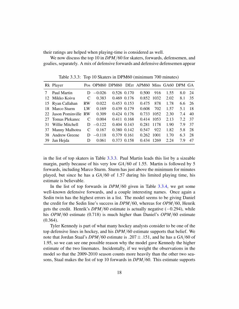
their ratings are helped when playing-time is considered as well.We now discuss the top 10 in DPM/60 for skaters, forwards, defensemen, and

goalies, separately. A mix of defensive forwards and defensive defensemen appear

Table 3.3.3: Top 10 Skaters in DPM60 (minimum 700 minutes)

Rk Player Pos OPM60 DPM60 DErr APM60 Mins GA60 DPM GA

7 Paul Martin D −0.026 0.526 0.170 0.500 916 1.55 8.0 2412 Mikko Koivu C 0.383 0.469 0.176 0.852 1032 2.02 8.1 3515 Ryan Callahan RW 0.022 0.453 0.153 0.475 878 1.78 6.6 2618 Marco Sturm LW 0.169 0.439 0.179 0.608 702 1.57 5.1 1822 Jason Pominville RW 0.309 0.424 0.176 0.733 1052 2.30 7.4 4027 Tomas Plekanec C 0.004 0.411 0.168 0.414 1053 2.13 7.2 3731 Willie Mitchell D −0.122 0.404 0.143 0.281 1178 1.90 7.9 3737 Manny Malhotra C 0.167 0.380 0.142 0.547 922 1.82 5.8 2838 Andrew Greene D −0.118 0.379 0.161 0.262 1001 1.70 6.3 2839 Jan Hejda D 0.061 0.373 0.158 0.434 1269 2.24 7.9 47

in the list of top skaters in Table 3.3.3. Paul Martin leads this list by a sizeablemargin, partly because of his very low GA/60 of 1.55. Martin is followed by 5forwards, including Marco Sturm. Sturm has just above the minimum for minutesplayed, but since he has a GA/60 of 1.57 during his limited playing time, hisestimate is believable.

In the list of top forwards in DPM/60 given in Table 3.3.4, we get somewell-known defensive forwards, and a couple interesting names. Once again aSedin twin has the highest errors in a list. The model seems to be giving Danielthe credit for the Sedin line’s success in DPM/60, whereas for OPM/60, Henrikgets the credit. Henrik’s DPM/60 estimate is actually negative (−0.294), whilehis OPM/60 estimate (0.718) is much higher than Daniel’s OPM/60 estimate(0.364).

Tyler Kennedy is part of what many hockey analysts consider to be one of thetop defensive lines in hockey, and his DPM/60 estimate supports that belief. Wenote that Jordan Staal’s DPM/60 estimate is .207± .151, and he has a GA/60 of1.95, so we can see one possible reason why the model gave Kennedy the higherestimate of the two linemates. Incidentally, if we weight the observations in themodel so that the 2009-2010 season counts more heavily than the other two sea-sons, Staal makes the list of top 10 forwards in DPM/60. This estimate supports

18

Table 3.3.4: Top 10 Forwards in DPM60 (minimum 700 minutes)

Rk Player Pos OPM60 DPM60 DErr APM60 Mins GA60 DPM GA

12 Mikko Koivu C 0.383 0.469 0.176 0.852 1032 2.02 8.1 3515 Ryan Callahan RW 0.022 0.453 0.153 0.475 878 1.78 6.6 2618 Marco Sturm LW 0.169 0.439 0.179 0.608 702 1.57 5.1 1822 Jason Pominville RW 0.309 0.424 0.176 0.733 1052 2.30 7.4 4027 Tomas Plekanec C 0.004 0.411 0.168 0.414 1053 2.13 7.2 3737 Manny Malhotra C 0.167 0.380 0.142 0.547 922 1.82 5.8 2841 Tyler Kennedy C 0.343 0.365 0.163 0.708 730 1.75 4.4 2142 David Krejci C 0.281 0.361 0.189 0.642 912 1.89 5.5 2944 Travis Moen LW −0.323 0.350 0.152 0.028 969 1.84 5.7 3045 Daniel Sedin LW 0.364 0.346 0.231 0.710 1057 2.03 6.1 36

his nomination for the 2009-2010 Selke trophy, which is given each season to thetop defensive forward in the game.

Mike Weaver and Mike Lundin are members of the list of top defensemen inDPM/60, which is shown in Table 3.3.5. Weaver has the second lowest GA/60 inthis list at 1.73, and his most common teammates, Chris Mason (2.31) and CarloColaiacovo (2.41) have a higher GA/60, so we see one reason why the modelgave him a high DPM/60 rating. Similarly, Lundin’s GA/60, while not as low

Table 3.3.5: Top 10 Defensemen in DPM60 (minimum 700 minutes)

Rk Player Pos OPM60 DPM60 DErr APM60 Mins GA60 DPM GA

7 Paul Martin D −0.026 0.526 0.170 0.500 916 1.55 8.0 2431 Willie Mitchell D −0.122 0.404 0.143 0.281 1178 1.90 7.9 3738 Andrew Greene D −0.118 0.379 0.161 0.262 1001 1.70 6.3 2839 Jan Hejda D 0.061 0.373 0.158 0.434 1269 2.24 7.9 4746 Mike Weaver D −0.419 0.341 0.153 −0.078 819 1.73 4.7 2462 Nicklas Lidstrom D 0.242 0.307 0.191 0.549 1374 1.82 7.0 4267 Tobias Enstrom D −0.005 0.301 0.166 0.296 1319 2.70 6.6 5968 Sean O’donnell D 0.027 0.298 0.133 0.325 1180 1.75 5.9 3469 Mike Lundin D −0.035 0.297 0.157 0.263 738 2.14 3.7 2670 Marc-E Vlasic D 0.030 0.296 0.150 0.326 1311 1.89 6.5 41

19

as Weaver’s, is still fairly low, despite the fact that his most common teammateshave a very high GA/60 (Mike Smith, 2.44; Vincent Lecavalier, 3.03; MartinSt. Louis, 2.97). Also, according to Gabriel Desjardins’ Quality of Competition(QualComp) statistic from Desjardins (2010), Lundin had the highest QualCompin 2009-2010 among players with at least 10 games played, indicating that heperformed well against strong competition.

Table 3.3.6: Top 10 Goalies in DPM60 (minimum 700 minutes)

Rk Player Pos OPM60 DPM60 DErr APM60 Mins GA60 DPM GA

1 Pekka Rinne G NA 0.845 0.232 0.845 1680 2.12 23.7 592 Dan Ellis G NA 0.757 0.218 0.757 1509 2.32 19.0 5814 Chris Mason G NA 0.460 0.169 0.460 2384 2.31 18.3 9224 Marty Turco G NA 0.424 0.154 0.424 2787 2.27 19.7 10529 Erik Ersberg G NA 0.410 0.199 0.410 728 2.14 5.0 2630 H. Lundqvist G NA 0.410 0.220 0.410 3223 2.10 22.0 11334 Jonathan Quick G NA 0.394 0.187 0.394 1781 2.15 11.7 6454 Cam Ward G NA 0.317 0.151 0.317 2655 2.23 14.0 9975 Tuukka Rask G NA 0.293 0.259 0.293 763 1.70 3.7 2276 Ty Conklin G NA 0.293 0.178 0.293 1392 2.13 6.8 49

Interestingly, the top 3 goalies in DPM/60, as shown in Table 3.3.6, haveplayed for the Nashville Predators at some point during the past three seasons.There are a couple possible reasons for this trend. One reason is that the estimatesare noisy, so it could simply be a coincidence that those three goalies ended up atthe top of this list. The estimates for Rinne and Ellis are significantly higher thanthose of the other goalies, but several other goalies are within one standard errorof the top 3 in DPM/60, and a few are within two standard errors of the top spot.Note that the low end of the 95% confidence intervals of the DPM/60 estimatesfor Rinne and Ellis are still in the top 7 in DPM/60, suggesting that, at worst, theywere still very good.

Even if the goalies’ DPM/60 estimates were not noisy, DPM/60 would stillnot be the best way to isolate and measure goalie’s individual ability. Recall thatthe interpretation of a goalie’s DPM/60 is goals per 60 minutes contributed bythe goalie on defense, or goals per 60 minutes prevented by the goalie. We couldthink of DPM/60 as measuring the difference between a goalie’s goals againstaverage at even strength and the league’s goals against average at even strength,

20

while adjusting for the strength of the teammates and opponents of the goalie. Agoalie who has a relatively low goals against average at even strength should ingeneral have a relatively high (good) DPM/60 estimate. In general, this relation-ship is true for our results. In Table 3.3.6, the 10 goalies with the highest DPM/60estimates also have low GA/60 statistics.

Unfortunately, goals against average is not the best measure of a goalie’s abil-ity. The number of goals per 60 minutes allowed by a team depends on not onlythe goalie’s ability at stopping shots on goal, but also the frequency and quality ofthe shots on goal that his team allows. So goals against average is a measure notjust of a goalie’s ability, but also of his team’s ability at preventing shots on goal.Ideally, the model would be able to correctly determine if the goalie or the teamin front of him deserves credit for a low goals against average, but that does notseem to be happening. One reason could be the relatively low number of goalieson each team. Another reason could be that there is some team-level effect not ac-counted for. If we include team variables in the model, the results are even worse.The team estimates are very noisy (with errors around 0.50), the goalie estimatesare even noisier with the team variables than without the team variables, and themodel still does not isolate a goalie’s ability.

Different techniques for measuring a goalie’s ability and contribution to histeam would be preferred over DPM/60. Most methods would likely use differentinformation, including the quality and frequency of the shots on goal that histeam allows. See, for example, Ken Krzywicki’s shot quality model in Krzywicki(2005) and Krzywicki (2009).

3.4 DPM

Recall that DPM is a measure of the defensive contribution of a player at even-strength in terms of goals over an entire season. We now discuss the top 10 play-ers, skaters, forwards, and defensemen in DPM. The list of top players in DPMgiven in Table 3.4.1 is entirely made up of goalies, which is not unexpected. Manypeople consider goalie the most important position in hockey, and this list seems tosupport that claim, at least for the defensive component of the game. While manygoalies have a lower DPM/60 than many skaters, the comparatively high minutesplayed for goalies bump many of them to the top of the list in DPM. Another con-sequence of the high minutes played is that the standard errors for goalies are nowvery high for DPM. This fact makes the DPM estimates for goalies less reliablethan the DPM estimates for skaters. We reiterate what we discussed at the endof Section 3.3: other methods of rating goalies are preferred over DPM/60 and

21

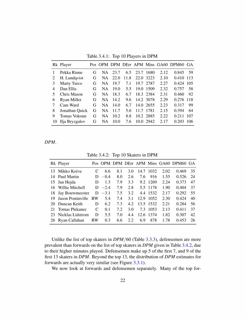
Table 3.4.1: Top 10 Players in DPM

Rk Player Pos OPM DPM DErr APM Mins GA60 DPM60 GA

1 Pekka Rinne G NA 23.7 6.5 23.7 1680 2.12 0.845 592 H. Lundqvist G NA 22.0 11.8 22.0 3223 2.10 0.410 1133 Marty Turco G NA 19.7 7.1 19.7 2787 2.27 0.424 1054 Dan Ellis G NA 19.0 5.5 19.0 1509 2.32 0.757 585 Chris Mason G NA 18.3 6.7 18.3 2384 2.31 0.460 926 Ryan Miller G NA 14.2 9.6 14.2 3078 2.29 0.276 1187 Cam Ward G NA 14.0 6.7 14.0 2655 2.23 0.317 998 Jonathan Quick G NA 11.7 5.6 11.7 1781 2.15 0.394 649 Tomas Vokoun G NA 10.2 8.8 10.2 2885 2.22 0.211 10710 Ilja Bryzgalov G NA 10.0 7.6 10.0 2942 2.17 0.203 106

DPM.

Table 3.4.2: Top 10 Skaters in DPM

Rk Player Pos OPM DPM DErr APM Mins GA60 DPM60 GA

13 Mikko Koivu C 6.6 8.1 3.0 14.7 1032 2.02 0.469 3514 Paul Martin D −0.4 8.0 2.6 7.6 916 1.55 0.526 2415 Jan Hejda D 1.3 7.9 3.3 9.2 1269 2.24 0.373 4716 Willie Mitchell D −2.4 7.9 2.8 5.5 1178 1.90 0.404 3718 Jay Bouwmeester D −3.1 7.5 3.2 4.4 1532 2.17 0.292 5519 Jason Pominville RW 5.4 7.4 3.1 12.9 1052 2.30 0.424 4020 Duncan Keith D 6.2 7.3 4.2 13.5 1532 2.21 0.284 5621 Tomas Plekanec C 0.1 7.2 3.0 7.3 1053 2.13 0.411 3723 Nicklas Lidstrom D 5.5 7.0 4.4 12.6 1374 1.82 0.307 4226 Ryan Callahan RW 0.3 6.6 2.2 6.9 878 1.78 0.453 26

Unlike the list of top skaters in DPM/60 (Table 3.3.3), defensemen are moreprevalent than forwards on the list of top skaters in DPM given in Table 3.4.2, dueto their higher minutes played. Defensemen make up 5 of the first 7, and 9 of thefirst 13 skaters in DPM. Beyond the top 13, the distribution of DPM estimates forforwards are actually very similar (see Figure 3.3.1).

We now look at forwards and defensemen separately. Many of the top for-

22

Table 3.4.3: Top 10 Forwards in DPM

Rk Player Pos OPM DPM DErr APM Mins GA60 DPM60 GA

13 Mikko Koivu C 6.6 8.1 3.0 14.7 1032 2.02 0.469 3519 Jason Pominville RW 5.4 7.4 3.1 12.9 1052 2.30 0.424 4021 Tomas Plekanec C 0.1 7.2 3.0 7.3 1053 2.13 0.411 3726 Ryan Callahan RW 0.3 6.6 2.2 6.9 878 1.78 0.453 2633 Pavel Datsyuk C 15.4 6.2 3.5 21.6 1186 1.84 0.314 3635 Daniel Sedin LW 6.4 6.1 4.1 12.5 1057 2.03 0.346 3639 Manny Malhotra C 2.6 5.8 2.2 8.4 922 1.82 0.380 2841 D. Langkow C −0.4 5.7 2.8 5.2 1010 2.02 0.336 3443 Travis Moen LW −5.2 5.7 2.5 0.4 969 1.84 0.350 3045 David Krejci C 4.3 5.5 2.9 9.8 912 1.89 0.361 29

wards in Table 3.4.3 are known to be very solid defensive forwards. Mikko Koivuis often praised for his work defensively, and Pavel Datsyuk is a two-time SelkeTrophy winner for the best defensive forward in the league. Jason Pominville’sranking is surprising given that his GA/60 is the worst among players on this list.Checking his most common linemates, we find Ryan Miller (2.29 GA/60), JochenHecht (2.64), and Toni Lydman (2.36), whose GA/60 are not significantly differ-ent than Pominville’s. Pominville did lead his team in traditional plus-minus in2007-2008 (+16), and was tied for second in 2009-2010 (+13), which may havecaused the high rating, but he was also a −4 in 2008-2009.

Paul Martin, the leader among skaters in DPM/60, tops the list of best de-fensemen in DPM given in Table 3.4.4, despite much lower minutes played thanthe others. Martin has a nice list of most common teammates (Martin Brodeur,1.92 GA/60; Johnny Oduya, 2.00; Zach Parise, 1.74) but his GA/60 is extremelylow, which is probably the cause of his low DPM/60 and DPM estimates. TobiasEnstrom’s DPM/60 and DPM estimates are high given that his 2.70 GA/60 and59 GA statistics are the worst in the list. Enstrom’s GA/60 is not significantlydifferent than the GA/60 of his most common linemates, Niclas Havelid (2.87GA/60), Johan Hedberg (2.67), and Kari Lehtonen (2.63). Further down En-strom’s list of common linemates is Ilya Kovalchuk, whose 3.09 GA/60 and −4.2DPM are among the worst in the league. All teammates (and opponents) affect themodel’s estimates, not just the three most common teammates, so Kovalchuk andsome other teammates with low defensive abilities could be increasing Enstrom’s

23

Table 3.4.4: Top 10 Defensemen in DPM

Rk Player Pos OPM DPM DErr APM Mins GA60 DPM60 GA

14 Paul Martin D −0.4 8.0 2.6 7.6 916 1.55 0.526 2415 Jan Hejda D 1.3 7.9 3.3 9.2 1269 2.24 0.373 4716 Willie Mitchell D −2.4 7.9 2.8 5.5 1178 1.90 0.404 3718 Jay Bouwmeester D −3.1 7.5 3.2 4.4 1532 2.17 0.292 5520 Duncan Keith D 6.2 7.3 4.2 13.5 1532 2.21 0.284 5623 Nicklas Lidstrom D 5.5 7.0 4.4 12.6 1374 1.82 0.307 4227 Tobias Enstrom D −0.1 6.6 3.7 6.5 1319 2.70 0.301 5928 Marc-E Vlasic D 0.7 6.5 3.3 7.1 1311 1.89 0.296 4130 Andrew Greene D −2.0 6.3 2.7 4.4 1001 1.70 0.379 2836 Ron Hainsey D −2.9 6.1 2.9 3.2 1264 2.50 0.289 53

defensive estimates. Another Atlanta defensemen, Ron Hainsey, also has a highDPM given his raw statistics. Looking deeper, his 2.50 GA/60 is actually secondbest on his team among players with more than 700 minutes. Our model seemsto be saying that Hainsey, like Enstrom, is better than his raw statistics suggest,mostly because of the quality of teammates that he plays with.

3.5 APM/60

We now begin to look at the top players in the league in terms of APM/60 andAPM. Recall that APM/60 is a measure of the total (offensive and defensive)contribution of a player at even-strength in terms of net goals (goals for minusgoals against) per 60 minutes of playing time.

Datysuk, considered by many to be the best two-way player in the game, topsthe list of best players in APM/60 given in Table 3.5.1. Only two goalies makethe top 10. We plot the kernel density estimate for APM/60 and APM in Figure3.5.1 to get an idea of whether this trend continues outside the top 10. Forwardsseem to have higher estimates than goalies and defensemen. Note that the picturechanges slightly for APM, but defensemen still seem to have the lowest estimatesin general. Goalies seem to have the widest spread in APM, which is expectedbecause of their high minutes played.

We now discuss the estimates for forwards and defensemen separately, start-ing with the top forwards in APM/60 given in Table 3.5.2. Burrows’ case is an

24

Table 3.5.1: Top 10 Players in APM60 (minimum 700 minutes)

Rk Player Pos OPM60 DPM60 APM60 Err Mins NG60 APM NG

1 Pavel Datsyuk C 0.777 0.314 1.091 0.247 1186 1.55 21.6 312 Marian Gaborik RW 0.715 0.303 1.018 0.222 853 1.01 14.5 153 Mikko Koivu C 0.383 0.469 0.852 0.246 1032 0.52 14.7 94 Pekka Rinne G NA 0.845 0.845 0.232 1680 NA 23.7 NA7 Zach Parise LW 0.652 0.155 0.807 0.236 1164 1.20 15.6 239 Joe Thornton C 0.590 0.177 0.767 0.227 1222 1.08 15.6 2210 Sidney Crosby C 0.818 −0.052 0.766 0.212 1059 1.04 13.5 1811 Dan Ellis G NA 0.757 0.757 0.218 1509 NA 19.0 NA12 Tim Connolly C 0.501 0.244 0.745 0.247 710 0.90 8.8 1115 Alex Ovechkin LW 0.723 0.010 0.733 0.254 1262 1.42 15.4 30

Figure 3.5.1: Kernel Density Estimation for APM/60 Estimates and APM Esti-mates.

−0.5 0.0 0.5 1.0

0.0

0.5

1.0

1.5

2.0

N = 447 Bandwidth = 0.0659

Den

sity

APM/60 Estimates

Forwards

Defensemen

Goalies

−10 0 10 20 30

0.00

0.05

0.10

0.15

N = 447 Bandwidth = 0.872

Den

sity

APM Estimates

Forwards

Defensemen

Goalies

interesting one. He did not appear in the top 10 lists for OPM/60 or DPM/60,but makes the top APM/60 list for forwards in Table 3.5.2 with balanced offen-sive and defensive estimates. He has been playing frequently with the Sedin twinsthis year, so one might think his rating would be difficult to separate from thetwins’ estimates. However, on average over the last three years, the Sedins are not

25

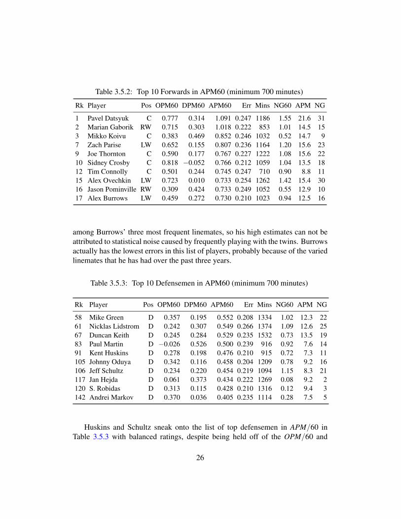
Table 3.5.2: Top 10 Forwards in APM60 (minimum 700 minutes)

Rk Player Pos OPM60 DPM60 APM60 Err Mins NG60 APM NG

1 Pavel Datsyuk C 0.777 0.314 1.091 0.247 1186 1.55 21.6 312 Marian Gaborik RW 0.715 0.303 1.018 0.222 853 1.01 14.5 153 Mikko Koivu C 0.383 0.469 0.852 0.246 1032 0.52 14.7 97 Zach Parise LW 0.652 0.155 0.807 0.236 1164 1.20 15.6 239 Joe Thornton C 0.590 0.177 0.767 0.227 1222 1.08 15.6 2210 Sidney Crosby C 0.818 −0.052 0.766 0.212 1059 1.04 13.5 1812 Tim Connolly C 0.501 0.244 0.745 0.247 710 0.90 8.8 1115 Alex Ovechkin LW 0.723 0.010 0.733 0.254 1262 1.42 15.4 3016 Jason Pominville RW 0.309 0.424 0.733 0.249 1052 0.55 12.9 1017 Alex Burrows LW 0.459 0.272 0.730 0.210 1023 0.94 12.5 16

among Burrows’ three most frequent linemates, so his high estimates can not beattributed to statistical noise caused by frequently playing with the twins. Burrowsactually has the lowest errors in this list of players, probably because of the variedlinemates that he has had over the past three years.

Table 3.5.3: Top 10 Defensemen in APM60 (minimum 700 minutes)

Rk Player Pos OPM60 DPM60 APM60 Err Mins NG60 APM NG

58 Mike Green D 0.357 0.195 0.552 0.208 1334 1.02 12.3 2261 Nicklas Lidstrom D 0.242 0.307 0.549 0.266 1374 1.09 12.6 2567 Duncan Keith D 0.245 0.284 0.529 0.235 1532 0.73 13.5 1983 Paul Martin D −0.026 0.526 0.500 0.239 916 0.92 7.6 1491 Kent Huskins D 0.278 0.198 0.476 0.210 915 0.72 7.3 11105 Johnny Oduya D 0.342 0.116 0.458 0.204 1209 0.78 9.2 16106 Jeff Schultz D 0.234 0.220 0.454 0.219 1094 1.15 8.3 21117 Jan Hejda D 0.061 0.373 0.434 0.222 1269 0.08 9.2 2120 S. Robidas D 0.313 0.115 0.428 0.210 1316 0.12 9.4 3142 Andrei Markov D 0.370 0.036 0.405 0.235 1114 0.28 7.5 5

Huskins and Schultz sneak onto the list of top defensemen in APM/60 inTable 3.5.3 with balanced ratings, despite being held off of the OPM/60 and

26

DPM/60 top 10 lists. We note that excluding goalies, Schultz’s most commonlinemates are Mike Green, Alexander Ovechkin, Nicklas Backstrom, and Alexan-der Semin. Schultz has accumulated fairly low goal and assist totals over the pastthree seasons while playing with some of league’s best offensive players, and yethis OPM/60 estimates are still high. In his case, the model may not be properlyseparating his offensive contribution from those of his teammates. It is also pos-sible that Schultz does a lot of little things on the ice that do not appear in boxscore statistics, but that contribute to his team’s offensive success nonetheless. Inhockey, it is difficult to separate offense and defense. A good defensive team,which can clear the puck from the defensive zone quickly, can help its offense byincreasing its time of possession. Likewise, a team with a good puck possessionoffense can help its defense by simply keeping the puck away from the opposi-tion. Time of possession data could help in separating offense and defense, butsuch data is not readily available. The model may or may not be doing a very goodjob of separating the two in some cases. See Pronman (2010) for a discussion byCorey Pronman about the connection between offense and defense.

3.6 APM

Recall that APM is a measure of the total (offensive and defensive) contributionof a player at even-strength in terms of net goals over an entire season. A hockeyfan familiar with the traditional plus-minus statistic can think of APM in the sameway, remembering that APM has been adjusted for both the strength of a player’steammates and the strength of his opponents. Goalies dominate the top of the listof best players in APM in Table 3.6.1, as is common with many of the advancedmetrics used by hockey analysts. This trend can also be seen in Figure 3.5.1.We reiterate again that other statistics are preferred over APM/60 and APM forestimating the contribution of goalies.

Pavel Datysuk has won the Selke Trophy in the 2007-08 and 2008-09 seasons,and is widely regarded as one of the top two-way players in the game, at leastamong forwards. He is third among players in APM, and he leads the list oftop skaters in Table 3.6.2 by a wide margin. It should also be pointed out thatall of the other players on this list are still within two standard errors of the topspot. Interestingly, Crosby and Ovechkin are the players with the lowest defensiveestimates on this list, which hurts their overall ratings.

Since forwards dominated the list in Table 3.6.2, we list the top 10 defensemenseparately in Table 3.6.3. The top 3 in DPM/60 (Table 3.3.5) are once again inthe top 3 here, though in a different order. One player we have not discussed is

27

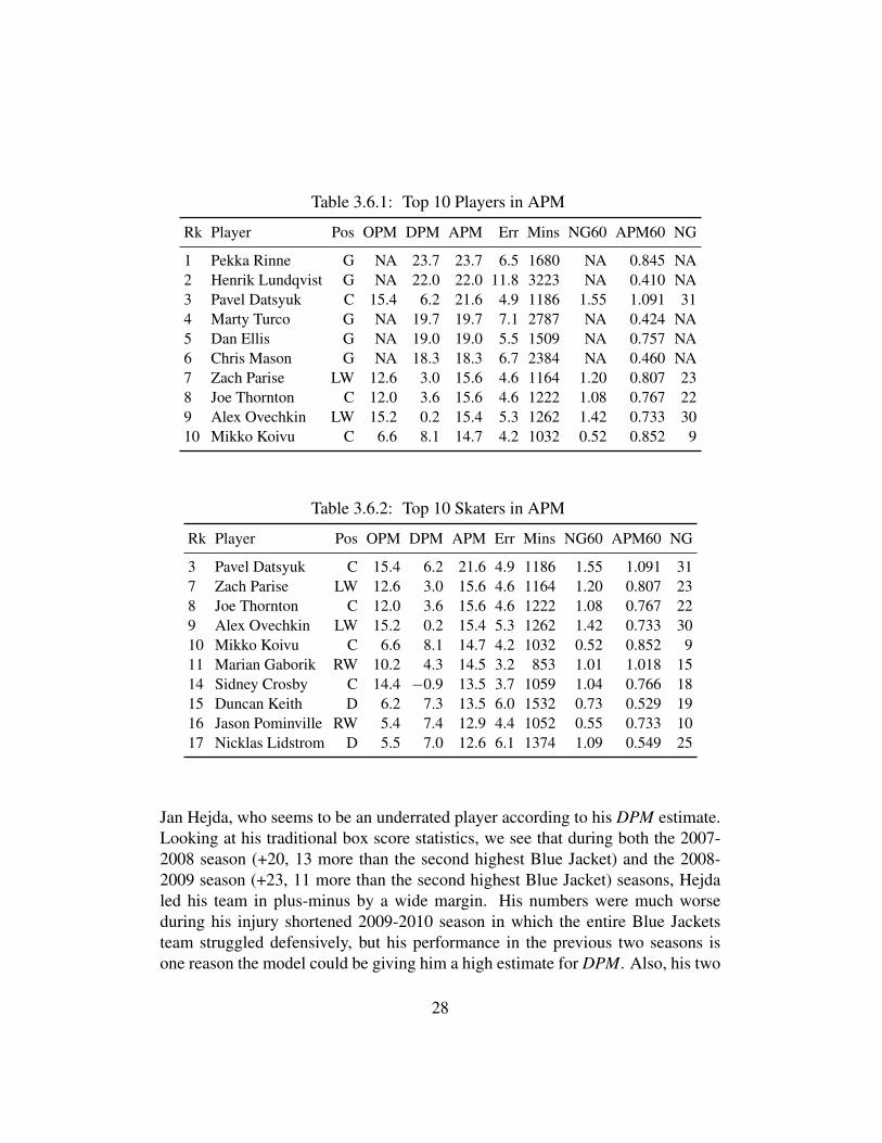
Table 3.6.1: Top 10 Players in APM

Rk Player Pos OPM DPM APM Err Mins NG60 APM60 NG

1 Pekka Rinne G NA 23.7 23.7 6.5 1680 NA 0.845 NA2 Henrik Lundqvist G NA 22.0 22.0 11.8 3223 NA 0.410 NA3 Pavel Datsyuk C 15.4 6.2 21.6 4.9 1186 1.55 1.091 314 Marty Turco G NA 19.7 19.7 7.1 2787 NA 0.424 NA5 Dan Ellis G NA 19.0 19.0 5.5 1509 NA 0.757 NA6 Chris Mason G NA 18.3 18.3 6.7 2384 NA 0.460 NA7 Zach Parise LW 12.6 3.0 15.6 4.6 1164 1.20 0.807 238 Joe Thornton C 12.0 3.6 15.6 4.6 1222 1.08 0.767 229 Alex Ovechkin LW 15.2 0.2 15.4 5.3 1262 1.42 0.733 3010 Mikko Koivu C 6.6 8.1 14.7 4.2 1032 0.52 0.852 9

Table 3.6.2: Top 10 Skaters in APM

Rk Player Pos OPM DPM APM Err Mins NG60 APM60 NG

3 Pavel Datsyuk C 15.4 6.2 21.6 4.9 1186 1.55 1.091 317 Zach Parise LW 12.6 3.0 15.6 4.6 1164 1.20 0.807 238 Joe Thornton C 12.0 3.6 15.6 4.6 1222 1.08 0.767 229 Alex Ovechkin LW 15.2 0.2 15.4 5.3 1262 1.42 0.733 3010 Mikko Koivu C 6.6 8.1 14.7 4.2 1032 0.52 0.852 911 Marian Gaborik RW 10.2 4.3 14.5 3.2 853 1.01 1.018 1514 Sidney Crosby C 14.4 −0.9 13.5 3.7 1059 1.04 0.766 1815 Duncan Keith D 6.2 7.3 13.5 6.0 1532 0.73 0.529 1916 Jason Pominville RW 5.4 7.4 12.9 4.4 1052 0.55 0.733 1017 Nicklas Lidstrom D 5.5 7.0 12.6 6.1 1374 1.09 0.549 25

Jan Hejda, who seems to be an underrated player according to his DPM estimate.Looking at his traditional box score statistics, we see that during both the 2007-2008 season (+20, 13 more than the second highest Blue Jacket) and the 2008-2009 season (+23, 11 more than the second highest Blue Jacket) seasons, Hejdaled his team in plus-minus by a wide margin. His numbers were much worseduring his injury shortened 2009-2010 season in which the entire Blue Jacketsteam struggled defensively, but his performance in the previous two seasons isone reason the model could be giving him a high estimate for DPM. Also, his two

28

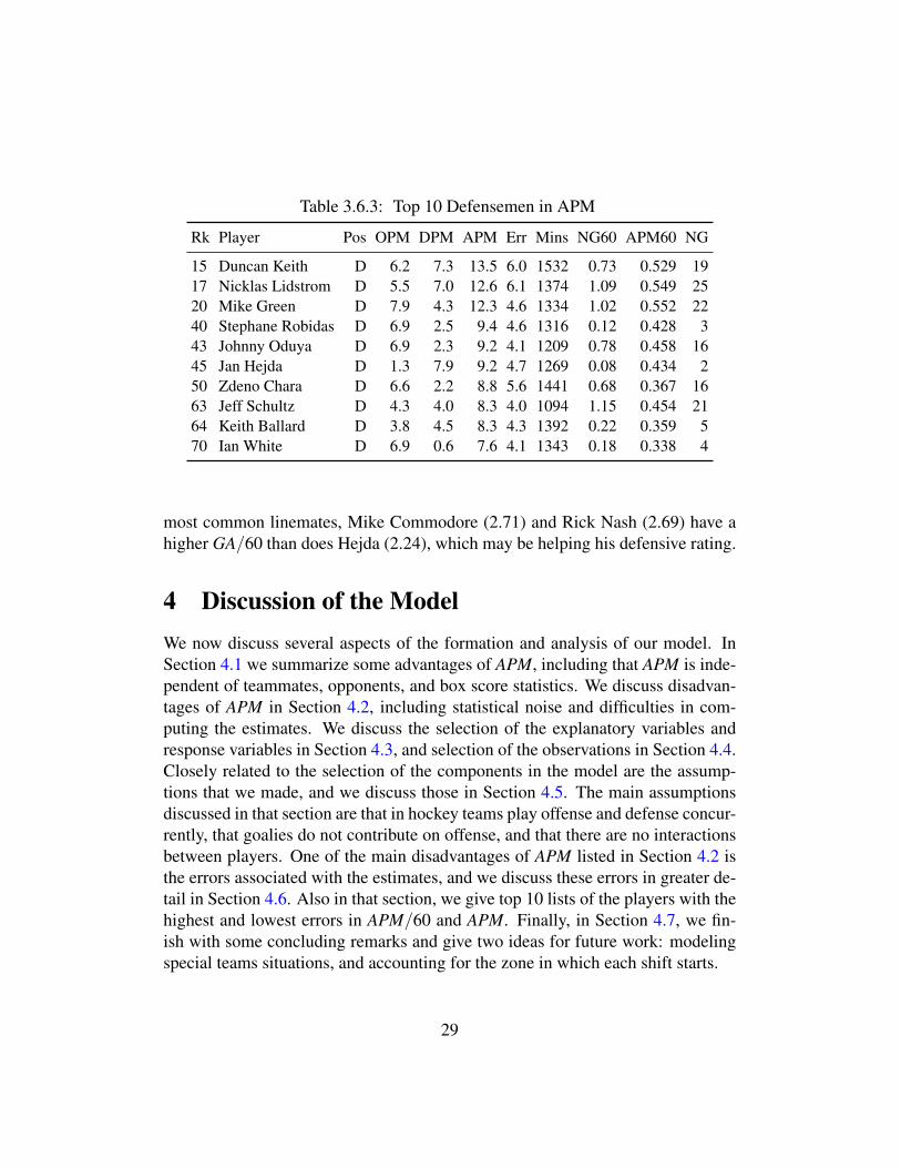
Table 3.6.3: Top 10 Defensemen in APM

Rk Player Pos OPM DPM APM Err Mins NG60 APM60 NG

15 Duncan Keith D 6.2 7.3 13.5 6.0 1532 0.73 0.529 1917 Nicklas Lidstrom D 5.5 7.0 12.6 6.1 1374 1.09 0.549 2520 Mike Green D 7.9 4.3 12.3 4.6 1334 1.02 0.552 2240 Stephane Robidas D 6.9 2.5 9.4 4.6 1316 0.12 0.428 343 Johnny Oduya D 6.9 2.3 9.2 4.1 1209 0.78 0.458 1645 Jan Hejda D 1.3 7.9 9.2 4.7 1269 0.08 0.434 250 Zdeno Chara D 6.6 2.2 8.8 5.6 1441 0.68 0.367 1663 Jeff Schultz D 4.3 4.0 8.3 4.0 1094 1.15 0.454 2164 Keith Ballard D 3.8 4.5 8.3 4.3 1392 0.22 0.359 570 Ian White D 6.9 0.6 7.6 4.1 1343 0.18 0.338 4

most common linemates, Mike Commodore (2.71) and Rick Nash (2.69) have ahigher GA/60 than does Hejda (2.24), which may be helping his defensive rating.

4 Discussion of the ModelWe now discuss several aspects of the formation and analysis of our model. InSection 4.1 we summarize some advantages of APM, including that APM is inde-pendent of teammates, opponents, and box score statistics. We discuss disadvan-tages of APM in Section 4.2, including statistical noise and difficulties in com-puting the estimates. We discuss the selection of the explanatory variables andresponse variables in Section 4.3, and selection of the observations in Section 4.4.Closely related to the selection of the components in the model are the assump-tions that we made, and we discuss those in Section 4.5. The main assumptionsdiscussed in that section are that in hockey teams play offense and defense concur-rently, that goalies do not contribute on offense, and that there are no interactionsbetween players. One of the main disadvantages of APM listed in Section 4.2 isthe errors associated with the estimates, and we discuss these errors in greater de-tail in Section 4.6. Also in that section, we give top 10 lists of the players with thehighest and lowest errors in APM/60 and APM. Finally, in Section 4.7, we fin-ish with some concluding remarks and give two ideas for future work: modelingspecial teams situations, and accounting for the zone in which each shift starts.

29

4.1 Advantages of APM

As with any metric of its kind, APM has its advantages and disadvantages. As wehave mentioned previously, the most important benefit of APM is that a player’sAPM does not depend on the strength of that player’s teammates or opponents.A major downside of the traditional plus-minus statistic is that it does depend onboth teammates and opponents, so it is not always a good measure of a player’sindividual contribution. For example, a player on a below-average team couldhave a traditional plus-minus that is lower than average simply because of thelinemates he plays with on a regular basis. An average player on a hypotheticalline with Wayne Gretzky and Mario Lemieux would probably have a traditionalplus-minus that is very high, but that statistic would not necessarily be a goodmeasure of his contribution to his team. On the other hand, the coefficients in ourmodel, which we use to estimate a player’s APM, are a measure of the contributionof a player when he is on the ice versus when he is off the ice, independent of allother players on the ice.

Another benefit of APM is that the estimate, in theory, incorporates all as-pects of the game, not just those areas that happen to be measured by box scorestatistics. Box score statistics do not describe everything that happens on the ice.For example, screening the goalie on offense and maintaining good positioningon defense are two valuable skills, but they are not directly measured using boxscore statistics. APM is like traditional plus-minus in that it attempts to measurehow a player effects the outcome on the ice in terms of goals scored by his teamon offense and goals allowed by his team on defense. A player’s personal totalsin goals, assists, points, hits, and blocked shots, for example, are never used incomputing APM. Nothing is assumed about the value of these box score statisticsand how they impact a player’s and a team’s performance.

Another benefit of our model is that we make minimal ad hoc assumptionsabout about which positions deserve the most credit for goal scoring or goal pre-vention. We do not assume, for example, that goalies or defensemen deservemore credit than forwards in goal prevention, or that forwards deserve more of thecredit when a goal is scored. From Figure 3.1.1, it seems that forwards contributemore than defensemen to goal scoring, but no such assumption was made duringthe formation of the model. The one assumption about position we did make inour first model in Section 2.1 was that goalies do not contribute on offense (seeSection 4.5.1).

30

4.2 Disadvantages of APM

One main drawback of the APM estimates is statistical noise. In particular, thestandard errors in the APM estimates for goalies are currently high. A priorityin future research is to take measures to reduce the errors. We discuss the errorsin detail in Section 4.6. Another drawback of APM is that the estimates do notinclude shootouts, and do not include the value of either penalties drawn by aplayer or penalties taken by a player. A team’s performance in shootouts has a bigimpact on their place in the standings. Shootout specialists can be very valuableto a team during the regular season, and ideally shootout performance would beaccounted for in APM. Penalties drawn and taken also impact the outcome ofa game. Penalties drawn by a player lead to more power plays for that player’steam, which in turn leads to more goals for his team. Likewise, penalties takenby a player lead to more power plays for, and more goals for, the opposing team.If the value of shootout performance, penalties drawn, and penalties taken wereestimated using another method that gives results the units of goals per game orgoals per season, those values could easily be combined with APM.

Another difficulty with APM is that the data required to calculate it is large,difficult to obtain in a usable form, and difficult to work with. Collecting and man-aging the data was easily the most time-consuming aspect of this research. Also,the data required for this model is only available (at least publicly) for very recentseasons. This model could not be used to estimate the value of Wayne Gretzky,Mario Lemieux, and Bobby Orr, for example, independent of their teammates andopponents.

The final downside to APM is that the model requires knowledge of linearregression or linear algebra, and is not easily computed from traditional statis-tics. The mathematics required makes the calculation of APM accessible to fewerhockey fans. It was a priority to ensure that at least the estimates themselves couldbe easily understood, even if the methods of calculating them are not.

4.3 Selection of the variablesWe now make a few remarks on how we chose the explanatory variables and theresponse variable in the model. For the model, we included players who playedmore than 4000 shifts during the 2007-2008, 2008-2009, and 2009-2010 seasons.In terms of minutes played, this cutoff is roughly 200 minutes per season on av-erage. Players with less than 4000 shifts during those seasons would have verynoisy estimates which would not be very reliable. Increasing the 4000 shift cutoff

31

would have reduced the errors slightly, but we would have also obtained estimatesfor fewer players.

In our model, the units of the coefficients are the same as the units of y. Wewanted to estimate a player’s contribution to his team in terms of goals per 60minutes, so we chose our response variable with those same units. The choice ofgoals per 60 minutes for the units of our estimates was important because we couldrate players based on this statistic, and we could also convert this rate statistic toa counting statistic, total goals over an entire season, using the minutes played byeach player. The resulting estimates have the units of goals, and they can be easilycompared with traditional plus-minus as well as advanced metrics already in ex-istence. Also, a priority was to ensure our estimates could be easily interpreted bythe average hockey fan. Since the units of APM are goals over an entire season,any hockey fan familiar with traditional plus-minus can understand the meaningof APM.

4.4 Selection of the observationsRecall that we define a shift to be a period of time during the game when thereare no substitutions made. During the 2007-2008, 2008-2009, and 2009-2010seasons, there were 990,861 shifts. We consider only shifts that take place ateven-strength (5-on-5, 4-on-4, 3-on-3), and we also require that two goalies be onthe ice. All power play and empty net situations were removed.

We noticed some errors in the data. There is a minimum of four players (count-ing goalies) and a maximum of 6 players (counting goalies) that can be on the icefor a team at the same time. However, for some shifts, there are less than fourplayers or more than six players on the ice for a team. These shifts may haveoccurred in the middle of a line change, during which it is difficult to record inreal-time which players are on or off the ice. Such shifts were removed. Wealso note that five games had missing data, and a few more games had incom-plete data, such as data for just one or two periods. The equivalent of about 10games of data is missing out of a total of 3,690 games during the three seasons inquestion. After removing shifts corresponding to empty net situations and specialteams situations, and shifts where errors were identified, 798,214 shifts remained.

4.5 Discussion of assumptionsSome of the assumptions used in the model require discussion. First, in our Ilardi-Barzilai-type model (Section 2.1), we split each shift into two observations, one

32

corresponding to the home team being on offense, and one corresponding to theaway team being on offense. We assume that in hockey a team plays offense anddefense concurrently during the entire shift, and we give the two observationsequal weight. This assumption of concurrency was suggested by Alan Ryder andwas used in Ryder (2004). In other sports, offense and defense are more distinctand more easily defined. However, because of the chaotic nature of play in hockey,defining what it means for a team to be on offense is tricky. Even if one coulddefine what it means to be “on offense”, the data needed to determine if a team ison offense might not be available.

Alteratively, we could say that the split into to two observations with equalweights was made by assuming that for each shift, a team was playing offensefor half the shift and playing defense for half the shift. One problem with thisassumption is that there may be some teams that spend more time with the puckthan without it.

4.5.1 Goalie contribution on offense

In our first model (Section 2.1), we ultimately decided to treat goalies differentlythan skaters by including only a defensive variable for each goalie. This decisionwas based on the the assumption that a goalie’s contribution on offense is negli-gible. This assumption is debatable. There are some great puck-handling goalies,and some poor ones, and that could affect both the offensive and defensive per-formance of their team. Some analysts have attempted to quantify the effects ofpuck handling for goalies and have come up with some interesting results. See,for example, Myrland (2010).

While we ultimately decided against including offensive variables for goalies,we did try the model both ways, and compared the results. We compared theoffensive results for skaters, and defensive results for both skaters and goalies.First, the defensive coefficients, the DPM results, and the errors associated withthem, stayed very similar for all skaters and goalies. The offensive coefficients,and the OPM estimates, stayed similar for most skaters when goalies were in-cluded, but in some extreme cases, the results varied greatly. For example, HenrikLundqvist’s offensive rating was extremely high, with very high errors. As a re-sult, the offensive results for several New York Rangers were significantly lowerwhen goalies were included. It was as if the model was giving Lundqvist muchof the credit for offensive production, while giving less credit to the skaters. Thestandard errors in OPM for these Rangers also increased. Similarly, three DetroitRed Wings goalies, Dominic Hasek, Chris Osgood, and Jimmy Howard, had very

33

low offensive ratings. Several Detroit players saw a significant boost in offensiveproduction when goalies were included. Once again, the errors for these playerssaw a significant increase.

One problem with these changes in offensive estimates is that the goalie rat-ings are extremely noisy and are not very reliable, so the effect that the goalieratings had on the skater ratings cannot be considered reliable either. On the otherhand, there could be some positives gained from including goalies. Recall thatwe do not consider empty net situations in our model, so anytime each skater ison the ice, he is on the ice with a goalie. For teams who rely very heavily onone goalie, that goalie could get 90% of the playing time for his team during theseason. That goalie’s variable could be acting similar to an indicator variable forthat team. So the goalie’s offensive estimates could be a measure of some sort ofteam-level effect, or coaching effect, on offensive production. For example, a lowestimate for a goalie’s OPM could be considered partially as an adjustment for anorganizational philosophy, or a coaching system, that favors a more conservative,defensive-minded approach.

In the end, we decided against including offensive variables for goalies in ourfirst model because of the noisiness of the goalies’ results, the effect that it hadon the skaters’ offensive ratings, the increase in interactions with other players,and the increase in errors that came with those changes. Note that in our secondmodel we do not have separate offensive and defensive variables for any of theplayers, including goalies, and goalies are considered on offense. So we have onemodel that does not include goalies for offensive purposes, and one model thatdoes. When we average the results of the two models, we balance the effects ofincluding goalies in one model, and excluding them in the other model.

4.5.2 Interactions between players

By not including interaction terms in the model, we do not account for interac-tions between players. Chemistry between two particular teammates, for exam-ple, is ignored in the model. The inclusion of interaction terms could reduce theerrors. The disadvantages of this type of regression would be that it is much morecomputationally intensive, and the results would be harder to interpret.

4.6 Discussion of ErrorsIn the introduction, and elsewhere in this paper, we noted that Henrik and DanielSedin have a much higher error than other players with a similar number of shifts.

34

One reason for this high error could be that the twin brothers spend most of theirtime on the ice together. Daniel spent 92% of his playing time with Henrik,the highest percentage of any other player combination where both players haveplayed over 700 minutes. Because of this high colinearity between the twins, itis difficult to separate the individual effect that each player has on the net goalsscored on the ice. It seems as though the model is giving Henrik the bulk of thecredit for the offensive contributions, and Daniel most of the credit for defense.Henrik’s defensive rating is strangely low given his low goals against while on theice. Likewise, Daniel’s offensive rating is unusually low.

Table 4.6.1: Top 10 Players in Highest Err in APM60 (minimum 700 minutes)

Rk Player Pos APM60 Err Mins Teammate.1 min1 Teammate.2 min2

69 Henrik Sedin C 0.424 0.328 1169 D.Sedin 83% R.Luongo 76%73 Daniel Sedin LW 0.710 0.326 1057 H.Sedin 92% R.Luongo 77%143 Ryan Getzlaf C 0.501 0.288 1116 C.Perry 83% J.Hiller 49%157 B. Morrow LW 0.141 0.283 805 M.Ribeiro 73% M.Turco 71%161 Corey Perry RW 0.370 0.282 1130 R.Getzlaf 82% J.Hiller 48%199 T. Holmstrom LW 0.175 0.269 724 P.Datsyuk 87% N.Lidstrom 51%205 N. Lidstrom D 0.549 0.266 1374 B.Rafalski 70% P.Datsyuk 49%210 David Krejci C 0.642 0.265 912 T.Thomas 60% B.Wheeler 49%218 N. Kronwall D 0.405 0.264 1055 B.Stuart 46% C.Osgood 46%221 Jason Spezza C 0.390 0.263 1075 D.Alfredss 60% D.Heatley 59%

The ten players with the highest error in APM/60 are shown in Table 4.6.1.Note that if we do not impose a minutes played minimum, the list is entirely madeup of players who played less than 200 minutes, so we have restricted this listto players that have played more than 700 minutes on average over the last threeseasons. The Sedins have significantly larger errors than the next players in thelist, and all of the players in this list are ones who spent a large percent of theirtime on the ice with a particular teammate or two.

In Table 4.6.2, we list the players with the lowest errors in APM/60. Goaliesdominate this list, partially because of playing time, and partially because goaliesshare the ice with a wider variety of players than skaters do. Also, with the ex-ception of Turco and Ward, all of the goalies in the list have the benefit of playingwith more than one team, further diversifying the number of players that theyhave played with. While goalies have lower errors in APM/60 than skaters do,

35

Table 4.6.2: Top 10 Players in Lowest Err in APM60 (minimum 700 minutes)

Rk Player Pos APM60 Err Mins Teammate.1 min1 Teammate.2 min2

1 Mike Smith G 0.222 0.144 1704 M.St. Loui 27% V.Lecavali 26%2 D. Roloson G 0.141 0.145 2259 T.Gilbert 24% S.Staios 24%3 Martin Biron G 0.012 0.149 2077 B.Coburn 28% K.Timonen 25%4 J. Labarbera G 0.165 0.150 1205 A.Kopitar 22% P.O’Sulliv 20%5 Cam Ward G 0.317 0.151 2655 E.Staal 32% T.Gleason 31%6 Alex Auld G 0.245 0.152 1409 C.Phillips 17% D.Heatley 15%7 A. Niittymaki G 0.177 0.154 1448 B.Coburn 19% K.Timonen 17%8 Ilja Bryzgalov G 0.203 0.154 2942 Z.Michalek 35% E.Jovanovs 32%9 Marty Turco G 0.424 0.154 2787 S.Robidas 35% T.Daley 35%10 Manny Legace G 0.253 0.155 1680 B.Jackman 28% E.Brewer 24%

that changes with playing-time dependent APM statistic (see Figure 4.6.1).If we remove goalies from consideration, we get the top 10 skaters in lowest

standard errors as shown in Table 4.6.3. Most of these players are defensemen

Table 4.6.3: Top 10 Skaters in Lowest Err in APM60 (minimum 700 minutes)

Rk Player Pos APM60 Err Mins Teammate.1 min1 Teammate.2 min2

20 J. Bouwmeester D 0.170 0.177 1532 T.Vokoun 50% M.Kiprusof 29%24 Olli Jokinen C 0.172 0.178 1165 T.Vokoun 30% M.Kiprusof 27%28 D. Seidenberg D 0.090 0.179 1067 C.Ward 45% T.Vokoun 28%29 C. Ehrhoff D 0.296 0.180 1285 E.Nabokov 54% R.Luongo 28%30 Ian White D 0.338 0.181 1343 V.Toskala 53% M.Stajan 30%31 Bryan Mccabe D 0.193 0.181 1172 T.Vokoun 53% V.Toskala 22%35 P. O’Sullivan C 0.074 0.183 1042 A.Kopitar 30% J.Labarber 23%36 Greg Zanon D 0.003 0.183 1307 D.Hamhuis 30% N.Backstro 27%39 Keith Ballard D 0.359 0.184 1392 T.Vokoun 48% D.Morris 23%40 Lee Stempniak RW 0.463 0.184 982 M.Legace 27% V.Toskala 25%

and have been on the ice for a high number of minutes. Every player in Table4.6.3 has played for two or more teams during the past three seasons. Stempniak,who has the lowest minutes played on the list, probably made the list because he

36

has played for three different teams. Also, Stempniak shared the ice with his mostcommon linemate, Manny Legace, for just 27% of his time on the ice.

We can look at the overall trend in APM/60 errors and APM errors in Figure4.6.1. The trends we noticed in the top 10 lists continue outside of the top 10. In

0.10 0.15 0.20 0.25 0.30 0.35 0.40 0.45

02

46

810

N = 447 Bandwidth = 0.01227

Den

sity

Errors in APM/60 Estimates

Forwards

Defensemen

Goalies

0 5 10

0.0

0.1

0.2

0.3

0.4

N = 447 Bandwidth = 0.218

Den

sity

Errors in APM Estimates

Forwards

Defensemen

Goalies

Figure 4.6.1: Kernel Density Estimation for APM/60 Errors and APM Errors.

particular, it appears that goalies tend to have the lowest errors in APM/60. Thedownside is that since many goalies get much more playing time than skaters,those goalies have much noisier APM estimates.

4.7 Future work and conclusionsWe highlight two improvements that could be made to our model. The most im-portant addition to this work would probably be to include a player’s offensive anddefensive contributions in special teams situations. While performance at even-strength is a good indicator of a player’s offensive and defensive value, someplayers seem to have much more value when they are on special teams. TeemuSelanne is an example of one player who has the reputation of being a power playgoal-scoring specialist, and we could quantify his ability using an estimate thatincludes special teams contributions.

37

Another improvement we could make is accounting for whether a shift startsin the offensive zone, defensive zone, or neutral zone, and accounting for whichteam has possession of the puck when the shift begins. The likelihood that a goalis scored during a shift is dependent on the zone in which a shift begins and isdependent on which team has possession of the puck when the shift begins. See,for example, Thomas (2006). This fact could be affecting the estimates of someplayers. Players who are relied upon for their defensive abilities, for example,may start many of their shifts in their own zone. This trend could result in moregoals against for those players than if they had started most of their shifts in theiroffensive zone. In the current model, there is no adjustment for this bias.

We believe that APM is a useful addition to the pool of hockey metrics alreadyin existence. The fact that APM is independent of teammates and opponents isthe main benefit of the metric. APM can be improved by addressing special teamsand initial zones, and reducing the statistical noise is a priority in future research.We hope that GM’s, coaches, hockey analysts, and fans will find APM a usefultool in their analysis of NHL players.

ReferencesAwad, T. (2009): “Understanding GVT, Part I,” URL http://www.

puckprospectus.com/article.php?articleid=233.

Boersma, C. (2007): “Corsi numbers,” URL http://hockeynumbers.

blogspot.com/2007/11/corsi-numbers.html.

Desjardins, G. (2010): “Behind The Net,” URL http://www.behindthenet.

com.

Fyffe, I. (2002): “Point Allocation,” URL http://hockeythink.com/

research/ptalloc.html.

Ilardi, S. and A. Barzilai (2008): “Adjusted Plus-Minus Ratings: New and Im-proved for 2007-2008,” URL http://www.82games.com/ilardi2.htm.

Krzywicki, K. (2005): “Shot quality model: A logistic regression approachto assessing nhl shots on goal,” URL http://www.hockeyanalytics.com/

Research_files/Shot_Quality_Krzywicki.pdf.

38

Krzywicki, K. (2009): “Removing observer bias from shot dis-tance - shot quality model - NHL regular season 2008-09,”URL http://www.hockeyanalytics.com/Research_files/

SQ-DistAdj-RS0809-Krzywicki.pdf.

Myrland, P. (2010): “In The Crease: Goalie Assists,” URL http://www.

puckprospectus.com/article.php?articleid=499.

NHL.com (2010): “The official website of the National Hockey League,” URLhttp://www.nhl.com/.

Pronman, C. (2010): “From Daigle to Datsyuk: The Tilted-Ice Effect,” URLhttp://www.puckprospectus.com/article.php?articleid=468.

Rosenbaum, D. (2004): “Measuring How NBA Players Help Their Teams Win,”URL http://www.82games.com/comm30.htm.

Ryder, A. (2004): “Player contribution,” URL http://www.hockeyanalytics.

com/Research_files/Player_Contribution_System.pdf.

Seppa, T. (2009): “Even strength total rating,” URL http://www.

puckprospectus.com/article.php?articleid=254.

Thomas, A. C. (2006): “The Impact of Puck Possession and Location on IceHockey Strategy,” Journal of Quantitative Analysis in Sports: Vol. 2 : Iss. 1,Article 6.

Witus, E. (2008): “Count the basket,” URL http://www.countthebasket.

com/blog/.

39