A Random-Key Genetic Algorithm for the Generalized Traveling

Salesman Problem

Lawrence V. Snyder ∗

Department of Industrial and Systems EngineeringLehigh University

200 West Packer Avenue, Mohler LabBethlehem, PA, 18015 USAlarry.snyder@lehigh.edu

Mark S. DaskinDepartment of Industrial Engineering and Management Sciences

Northwestern University2145 Sheridan Road, MEAS C210

Evanston, IL, 60208 USAm-daskin@northwestern.edu

February 25, 2005

Abstract

The Generalized Traveling Salesman Problem is a variation of the well known TravelingSalesman Problem in which the set of nodes is divided into clusters; the objective is to find aminimum-cost tour passing through one node from each cluster. We present an effective heuristicfor this problem. The method combines a genetic algorithm (GA) with a local tour improvementheuristic. Solutions are encoded using random keys, which circumvent the feasibility problemsencountered when using traditional GA encodings. On a set of 41 standard test problems withsymmetric distances and up to 442 nodes, the heuristic found solutions that were optimal inmost cases and were within 1% of optimality in all but the largest problems, with computationtimes generally within 10 seconds. The heuristic is competitive with other heuristics publishedto date in both solution quality and computation time.

Keywords: Traveling salesman, GTSP, Genetic algorithms, Random keys, Metaheuristics

∗Corresponding author.

1

1 INTRODUCTION 2

1 Introduction

1.1 The GTSP

The generalized traveling salesman problem (GTSP) is a variation of the well known

traveling salesman problem in which not all nodes need to be visited by the tour. In

particular, the set V of nodes is partitioned into m sets, or clusters, V1, . . . , Vm with

V1 ∪ . . . ∪ Vm = V and Vi ∩ Vj = ∅ if i 6= j. The objective is to find a minimum-length

tour containing exactly one node from each set Vi.

Applications of the GTSP include postal routing [19], computer file sequencing [16],

order picking in warehouses [27], process planning for rotational parts [5], and the

routing of clients through welfare agencies [35]. In addition, many other combinatorial

optimization problems can be reduced to, or have as a subproblem, the GTSP (see [19]).

The GTSP is NP-hard, since the TSP is a special case obtained by partitioning V into

|V | subsets, each containing one node. In this paper we present a heuristic approach to

solving the GTSP.

A given instance of the GTSP may use “symmetric” distances, in which the distance

from node i to node j is the same as the distance from j to i, or “asymmetric” distances;

there are theoretical and computational consequences of using one type of distance

metric or the other. For example, the GTSP is often transformed into an equivalent TSP,

but many such transformations depend on whether or not the problem is symmetric.

Similarly, a given algorithm’s computational performance may be quite different when

applied to different types of instances. We test our heuristic on a standard test-bed of

symmetric instances.

1 INTRODUCTION 3

1.2 Genetic Algorithms

A genetic algorithm (GA) is a metaheuristic inspired by the efficiency of natural selec-

tion in biological evolution. Genetic algorithms have been applied successfully to a wide

variety of combinatorial optimization problems and are the subject of numerous recent

books [26, 30, 39, 40, 41] and conference proceedings [1, 2, 4, 17]. Unlike traditional

heuristics (and some metaheuristics like tabu search) that generate a single solution

and work hard to improve it, GAs maintain a large number of solutions and perform

comparatively little work on each one. The collection of solutions currently under con-

sideration is called the population. Each member of the population (called an individual

or a chromosome) is an encoded version of a solution. The encoding strategy is differ-

ent for different optimization problems, and a given problem may have more than one

workable encoding strategy. The goal of any encoding is to translate a solution into a

string of genes that make up the chromosome, just as in biological genetics.

Each iteration of a GA consists of several operators that construct a new generation

of solutions from the old one in a manner designed to preserve the genetic material of the

better solutions (survival of the fittest). Many GA operators have been proposed; the

three most common are reproduction, crossover, and mutation. Reproduction consists

of simply copying the best solutions from the previous generation into the next, with

the intention of preserving very high-quality solutions in the population as-is. Crossover

takes two “parents,” randomly chosen, and produces one or more “offspring” that con-

tain some combination of genes from the parents. Crossover can be performed in a

deterministic manner (e.g., “one-point” crossover), with genes appearing before a cer-

tain cutoff coming from parent 1 and genes after the cutoff coming from parent 2, or in

a random manner, with each gene taken from a given parent with a certain probability.

1 INTRODUCTION 4

The mutation operator changes a few genes randomly, borrowing from the evolutionary

concept that random genetic mutations may produce superior offspring (or, of course,

inferior offspring, but such individuals are less likely to survive from one generation

to the next). Our algorithm does not use mutation, but rather immigration, in which

new individuals are generated randomly from scratch, rather than performing random

mutations on existing individuals.

Each iteration of a standard GA consists of generating a new population using the GA

operators. Our GA also uses judiciously applied local improvement heuristics to improve

the quality of the individuals in the population without adding excessive computation

time.

1.3 Random Keys

The GA presented in this paper uses random keys to encode solutions. The use of

random keys is described in [3] and is useful for problems that require permutations

of the integers and for which traditional one- or two-point crossover presents feasibility

problems. The technique is best illustrated with an example.

Consider a 5-node instance of the classical TSP. Traditional GA encodings of TSP

solutions consist of a stream of integers representing the order in which nodes are to be

visited by the tour. (That is, the solution 4 2 1 5 3 represents the tour 3 → 2 → 5 →

1 → 4, not the tour 4 → 2 → 1 → 5 → 3.) But one-point crossover, for example, may

result in children with some nodes visited more than once and others not visited at all.

For example, the parents1 4 3 2 52 4 5 3 1

might produce the children1 4 3 3 12 4 5 2 5

1 INTRODUCTION 5

In the random key method, we assign each gene a random number drawn uniformly

from [0, 1). To decode the chromosome, we visit the nodes in ascending order of their

genes. For example:

Random key 0.42 0.06 0.38 0.48 0.81Decodes as 3 1 2 4 5

(Ties are broken arbitrarily.) Nodes that should be early in the tour tend to “evolve”

genes closer to 0 and those that should come later tend to evolve genes closer to 1.

Standard crossover techniques will generate children that are guaranteed to be feasible.

1.4 Contributions

This paper contributes to the literature by presenting a heuristic for the GTSP that

uses a novel combination of features (GAs, random keys, and improvement heuristics).

Our heuristic finds optimal solutions for a large percentage of instances from a set

of standard test problems, with computation times that are competitive with, if not

superior to, previously published heuristics. We also present extensive computational

results lending insight into the behavior of the heuristic, such as the relative importance

of the GA and the improvement heuristics. Finally, like any GA, our heuristic is simple

to implement and can be easily modified to incorporate alternate objective functions or

additional constraints.

The remainder of this paper is organized as follows: Section 2 presents a brief lit-

erature review; section 3 describes the algorithm in greater detail; section 4 provides

computational results; and section 5 summarizes our findings and discusses avenues for

future research.

2 LITERATURE REVIEW 6

2 Literature Review

The earliest papers on the GTSP discuss the problem in the context of particular

applications [16, 35, 38]. Laporte, Mercure, and Nobert [20, 21] and Laporte and Nobert

[22] began to study exact algorithms and some theoretical aspects of the problem in

the 1980s. Since then, a few dozen papers related to the GTSP have appeared in the

literature. Fischetti, Salazar-Gonzalez, and Toth [13] discuss facet-defining inequalities

for the GTSP polytope, and in a later paper [14] use the polyhedral results to develop a

branch-and-cut algorithm. Other exact algorithms are presented in [28] (a Lagrangian-

based branch-and-bound algorithm) and [7] (a dynamic programming algorithm).

A variety of descriptions of the GTSP are present in the literature. Some papers

assume symmetry or the triangle inequality; others do not. Some require the subsets to

form a strict partition of the node set; others allow them to overlap. Most papers allow

the tour to visit more than one node per cluster, but some require that exactly one

node per cluster be visited. (The two formulations are equivalent if the distance matrix

satisfies the triangle inequality.) Only a few papers (see [22, 35]) handle fixed costs for

including a node on the tour, possibly because such fixed costs can be incorporated into

the distance costs via a simple transformation (see [22]; note that this transformation

does not preserve the triangle inequality).

Applications of the GTSP are discussed in [5, 19, 27]. [12] transforms the clustered

rural postman problem into the GTSP. [6, 9, 23, 25, 29] present transformations of the

GTSP into standard TSP instances that can then be solved using TSP algorithms and

heuristics. Some of the resulting TSP instances have nearly the same number of nodes

as the original GTSP instances and have nice properties like symmetry and the triangle

inequality; others have many more nodes and are more irregular. Some transformations

2 LITERATURE REVIEW 7

of the GTSP into the TSP (e.g., that in [29]) have the property that an optimal solution

to the related TSP can be converted to an optimal solution to the GTSP, but a (sub-

optimal) feasible solution for the TSP may not be feasible for the GTSP, reinforcing the

necessity for good heuristics for the GTSP itself. Furthermore, well known heuristics

for the TSP may not perform well for the GTSP; for example, “generalized” versions of

Christofides’s heuristic have worst-case bounds that are strictly greater than its worst-

case bound of 32 for the TSP [11, 36].

Two approximation algorithms have been published for the GTSP. Slavık [36] de-

velops a 3ρ/2-approximation algorithm for the GTSP, where ρ is the number of nodes

in the largest cluster, that is, ρ = maxi=1,...,m{|Vi|}. As ρ may be quite large, the

worst-case bound may be relatively weak. Garg, Konjevod, and Ravi [15] present an

approximation algorithm for the group Steiner tree problem, which provides as a byprod-

uct an O(log2 |V | log log |V | log m)-approximation algorithm for the GTSP. Both papers

assume that the distance matrix satisfies the triangle inequality.

Noon [27] proposed several heuristics for the GTSP, the most promising of which

is an adaptation of the well known nearest-neighbor heuristic for the TSP. Fischetti,

Salazar-Gonzalez, and Toth [14] propose similar adaptations of the farthest-insertion,

nearest-insertion, and cheapest-insertion heuristics.

Renaud and Boctor [32] develop the most sophisticated heuristic published to date,

which they call GI3 (Generalized Initialization, Insertion, and Improvement). GI3 is a

generalization of the I3 heuristic proposed in [33]. It consists of three phases. The first,

Initialization, constructs an initial tour by choosing one node from each cluster that is

“close” to the other clusters, then greedily building a tour that passes through some, but

not necessarily all, of the chosen nodes. The second phase, Insertion, completes the tour

3 THE HEURISTIC 8

by successively inserting nodes from unvisited clusters in the cheapest possible manner

between two consecutive clusters on the tour, allowing the visited node to change for

the adjacent clusters; after each insertion, the heuristic performs a modification of the

3-opt improvement method. The third phase, Improvement, uses modifications of 2-opt

and 3-opt to improve the tour. The modifications, called G2-opt, G3-opt, and G-opt,

allow the visited nodes from each cluster to change as the tour is being re-ordered by

the 2-opt or 3-opt procedures.

Several researchers (see [18] and the references contained within) have implemented

GAs for the standard TSP, with mixed results. The GA in [18] found new best solutions

for some well studied benchmark problems.

3 The Heuristic

Our heuristic couples a GA much like that described in [3] with a local improvement

heuristic. We will describe the heuristic in the context of the symmetric GTSP; the

heuristic can be modified easily to handle problems with asymmetric distance matrices,

though our computational results do not necessarily generalize to the asymmetric case.

Throughout the rest of this paper, we will use the terms “solution,” “individual,” and

“chromosome” interchangeably to refer to either a GTSP tour or its representation in

the GA.

3.1 Encoding and Decoding

Bean [3] suggests encoding the GTSP as follows: each set Vi has a gene consisting of an

integer part (drawn from {1, . . . , |Vi|}) and a fractional part (drawn from [0, 1)). The

integer part indicates which node from the cluster is included on the tour, and the nodes

3 THE HEURISTIC 9

are sorted by their fractional part as described in section 1.3 to indicate the order.

For example, consider a GTSP instance with V = {1, . . . , 20} and V1 = {1, . . . , 5}, . . . ,

V4 = {16, . . . , 20}. The random key encoding

4.23 3.07 1.80 3.76

decodes as the tour 8 → 4 → 18 → 11: the integer parts of the genes decode as,

respectively, node 4, node 8 (the third node in V2), node 11 (the first node in V3), and

node 18 (the third node in V4), and the fractional parts, when sorted, indicate that the

clusters should be visited in the order 2 → 1 → 4 → 3.

The GA operators act directly on the random key encoding. When tour improve-

ments are made, the encoding must be adjusted to account for the new solution (see

section 3.4 below).

The population is always stored in order of objective value, from best to worst.

3.2 Initial Population

The initial population is created by generating a population consisting of N chromo-

somes (we use N = 100), drawing the gene for set Vi uniformly from [1, |Vi| + 1) (or,

equivalently, adding an integer drawn randomly from {1, . . . , |Vi|} to a real number

drawn randomly from [0, 1)). “Level-I” improvement heuristics (see section 3.4) are

applied to each individual in the population.

3.3 GA Operators

At each generation, 20% of the population comes directly from the previous population

via reproduction; 70% is spawned via crossover; and the remaining 10% is generated

via immigration. We describe each of these operators next.

3 THE HEURISTIC 10

3.3.1 Reproduction

Our algorithm uses an elitist strategy of copying the best solutions in the population to

the next generation. This guarantees monotonic non-degradation of the best solution

from one generation to the next and ensures a constant supply of good individuals for

mating.

3.3.2 Crossover

We use parametrized uniform crossover [37] to generate offspring. First, two parents

are chosen at random from the old population. One child is generated from the two

parents, and it inherits each gene from parent 1 with probability 0.7 and from parent 2

with probability 0.3.

3.3.3 Immigration

A small number of new individuals are created in each generation using the technique

described in section 3.2. Like the more typical mutation operator, this immigration

operator helps ensure a diverse population.

3.4 Improvement Heuristics

Local improvement heuristics have been shown by various researchers to add a great

deal of power to GAs (see, for example, [24]). In our algorithm, every time a new

individual is created, either during crossover or immigration or during the construction

of the initial population, we attempt to improve the solution using 2-opt and “swap”

operations.

The well known 2-opt heuristic attempts to find two edges of the tour that can be

3 THE HEURISTIC 11

removed and two edges that can be inserted to obtain a single tour with lower cost. For

problems with Euclidean distances, a 2-opt exchange “straightens” a tour that crosses

itself.

The “swap” operation involves removing the node from cluster Vi and inserting a

different node from Vi into the tour. The insertion is done using a modified nearest-

neighbor criterion, so that the new node may be inserted on the tour in a spot different

from the original node. In pseudocode, the swap operation is as follows:

procedure SWAP(tour T ; set Vi; node j ∈ Vi, j ∈ T ; distances Duv betweeneach u, v ∈ V )

remove j from Tfor each k ∈ Vi

ck ← min{Duk + Dkv −Duv|(u, v) is an edge in T}k∗ ← argmink∈Vi

{ck}insert k∗ into T between the nodes u and v that attained the cost ck∗

Note that k∗ may be the same node as j, which allows the heuristic to move a node to

a different spot on the tour.

The 2-opt and swap operations are considered separately by our heuristic; they are

not integrated, as in the G2-opt, G3-opt, and G-opt methods used by [32].

When an improvement is made to the solution, the encoding must be altered to

reflect the new tour. We do this by rearranging the fractional parts of the genes to give

rise to the new tour. When a swap is performed, we must also adjust the integer part

of the gene for the affected set.

To take a simple example, suppose we have the chromosome

1.1 1.3 1.4 1.7

for the sets Vi given in section 3.1; this represents the tour 1 → 6 → 11 → 16. Now

suppose we perform a swap by replacing node 16 with node 17 and repositioning it after

3 THE HEURISTIC 12

node 1 so that the new tour is 1 → 17 → 6 → 11. The new encoding is

1.1 1.4 1.7 2.3.

For each individual in the population, we store both the original (pre-improvement)

cost and the final cost after improvements have been made. When a new individual

is created, we compare its pre-improvement cost to the pre-improvement cost of the

individual at position p × N in the previous (sorted) population, where p ∈ [0, 1] is a

parameter of the algorithm (we use p = 0.05 in our implementation). If the new solution

is worse than the pre-improvement cost of this individual we use level-I improvement:

apply one 2-opt exchange and one swap (assuming a profitable one can be found) and

store the resulting individual. If, on the other hand, the new solution is better, we use

level-II improvement: apply 2-opts until no profitable 2-opts can be found, then apply

swaps until no profitable swaps can be found, and repeat until no improvements have

been made in a given pass. This technique is designed to spend more time improving

solutions that seem promising in comparison to previous solutions and to spend less

time on the others. In both level-I and level-II improvement, we use a “first-improving”

strategy in which the first move of a given type that improves the objective value is

implemented, rather than searching for the best such move before choosing one.

No improvement is done during the reproduction phase, since these solutions have

already been improved.

3.5 Population Management

Two issues are worth mentioning regarding how we maintain GA populations. First,

no duplicates are allowed in the population. Each time a new individual is created, it

is compared to the individuals already in the population; if it matches one of them,

3 THE HEURISTIC 13

it is discarded and a new individual is created. Duplicate-checking is performed after

improvement, and individuals are considered identical if the decoded solutions are iden-

tical, not the genes. That is, chromosomes 2.14 4.25 3.50 2.68 and 2.07 4.73 3.81 2.99

are considered identical since they represent the same tour.

Second, it is undesirable to allow multiple “reflections” and “rotations” of a tour

to co-exist in the population. That is, if 1 → 6 → 11 → 16 is in the population, we

would not want 6 → 11 → 16 → 1 or 16 → 11 → 6 → 1 in the population. There

are two reasons for this. One is that such quasi-duplicates appear to add diversity to

the population but in fact do not, and so should be avoided just as duplicates are.

The second reason is that crossover between two such individuals will result in offspring

whose genetic information is “watered down” and may lead to slower convergence of the

GA. In the course of the GA, nodes that should appear consecutively in the tour tend

to evolve fractional parts of the gene that are close to one another. For this process

to work, the beginning of the tour needs to be well defined—that is, we can’t allow

reflections and rotations.

For example, suppose V = {1, . . . , 5} and Vi = {i} for all i, and suppose it is optimal

for nodes 3 and 4 to be consecutive on the tour. The chromosomes

1.1 1.9 1.3 1.4 1.81.4 1.8 1.5 1.7 1.2

represent the tours 1 → 3 → 4 → 5 → 2 and 5 → 1 → 3 → 4 → 2, respectively. Their

offspring might be1.4 1.9 1.3 1.7 1.8

representing the tour 3 → 1 → 4 → 5 → 2; nodes 3 and 4 are split. If, however, the

second solution had been rotated so that it began at node 1, its encoding would be

1.2 1.7 1.4 1.5 1.8

If this individual were to mate with the first one, it would produce offspring in which

4 COMPUTATIONAL RESULTS 14

the genes for nodes 3 and 4 were no more than 0.2 apart from one another, making it

more likely that these nodes would be consecutive.

To avoid rotations, we artificially set the fractional part of the gene for V1 to 0,

ensuring that set 1 will be at the beginning of the tour. To avoid reflections, we must

choose between the two orderings of a given tour that begin with cluster 1. The node

from V1 has two neighbors; we require the lower-indexed neighbor to appear in slot 2

on the tour (and the higher-indexed neighbor to appear in slot m). These rules ensure

that each tour is stored in a unique manner and that quasi-duplicates are eliminated.

3.6 Termination Criteria

The algorithm terminates when 100 iterations have been executed, or when 10 con-

secutive iterations have failed to improve the best-known solution. These numbers are

parameters that may easily be changed. (In our computational tests, the first criterion

never held—the GA always terminated because 10 consecutive iterations had failed

to improve the solution. We tested termination criteria greater than 10 on our test

problems and found substantially longer run times with little improvement in solution

quality.)

4 Computational Results

4.1 Experimental Design

Fischetti, Salazar-Gonzalez, and Toth [14] describe a branch-and-cut algorithm to solve

the symmetric GTSP. In their paper, they derive test problems by applying a partition-

ing method to 46 standard TSP instances from the TSPLIB library [31]. They provide

optimal objective values for each of the problems, and since the partitioning method

4 COMPUTATIONAL RESULTS 15

is deterministic and is described in enough detail to reproduce their test problems, we

were able to apply our heuristic to the same problems and compare the results.

We tested our algorithm on all of the problems discussed in [14] except the five

problems that use great-circle (geographical) distances. The problems we tested have

between 48 and 442 nodes; m is set to dn/5e in each case, where n is the number of

nodes and m is the number of clusters. Most of the problems use Euclidean distances,

but a few have explicit distance matrices given,1 and one uses a “modified Euclidean”

distance measure (see [31] for details); all distance matrices are symmetric. For each

problem, we ran the GA five times to examine the algorithm’s performance and its

variation from trial to trial. The algorithm was implemented in C++ and tested on a

Gateway Profile 4MX desktop computer with a Pentium IV 3.2 GHz processor and 1.0

GB RAM, running under Windows XP.

4.2 Solution Quality

Table 1 summarizes the results for each of the problems. The columns are as follows:

Problem: The name of the test problem. The digits at the beginning of the name givethe number of clusters (m); those at the end give the number of nodes (n).

Opt Obj Val: The optimal objective value for the problem, as reported in Table II of[14].

# Opt: The number of trials, out of five, in which the GA found the optimal solution

# Best: The number of trials, out of five, in which the GA found its best solution.(For problems in which an optimal solution was found, this is equal to the “#Opt” column.)

Mean, Minimum, Maximum: The mean, minimum, and maximum objective valuesreturned in the five trials (in the Value column), and the respective percentagesabove the optimal value (in the Pct column).

1The explicit distance matrices do not satisfy the triangle inequality. Nevertheless, the optimal solutions to the

GTSP for these problems contain exactly one node per set, allowing us to use the results from [14].

4 COMPUTATIONAL RESULTS 16

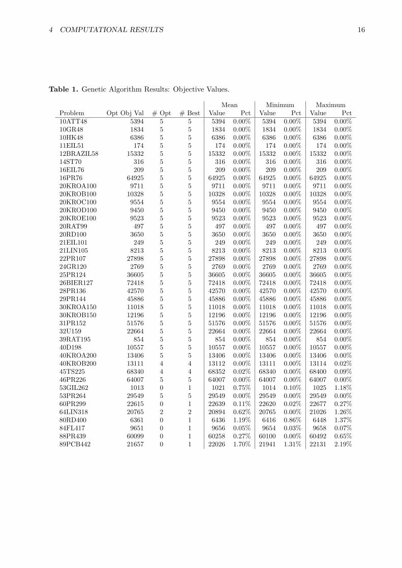
Table 1. Genetic Algorithm Results: Objective Values.

Mean Minimum MaximumProblem Opt Obj Val # Opt # Best Value Pct Value Pct Value Pct10ATT48 5394 5 5 5394 0.00% 5394 0.00% 5394 0.00%10GR48 1834 5 5 1834 0.00% 1834 0.00% 1834 0.00%10HK48 6386 5 5 6386 0.00% 6386 0.00% 6386 0.00%11EIL51 174 5 5 174 0.00% 174 0.00% 174 0.00%12BRAZIL58 15332 5 5 15332 0.00% 15332 0.00% 15332 0.00%14ST70 316 5 5 316 0.00% 316 0.00% 316 0.00%16EIL76 209 5 5 209 0.00% 209 0.00% 209 0.00%16PR76 64925 5 5 64925 0.00% 64925 0.00% 64925 0.00%20KROA100 9711 5 5 9711 0.00% 9711 0.00% 9711 0.00%20KROB100 10328 5 5 10328 0.00% 10328 0.00% 10328 0.00%20KROC100 9554 5 5 9554 0.00% 9554 0.00% 9554 0.00%20KROD100 9450 5 5 9450 0.00% 9450 0.00% 9450 0.00%20KROE100 9523 5 5 9523 0.00% 9523 0.00% 9523 0.00%20RAT99 497 5 5 497 0.00% 497 0.00% 497 0.00%20RD100 3650 5 5 3650 0.00% 3650 0.00% 3650 0.00%21EIL101 249 5 5 249 0.00% 249 0.00% 249 0.00%21LIN105 8213 5 5 8213 0.00% 8213 0.00% 8213 0.00%22PR107 27898 5 5 27898 0.00% 27898 0.00% 27898 0.00%24GR120 2769 5 5 2769 0.00% 2769 0.00% 2769 0.00%25PR124 36605 5 5 36605 0.00% 36605 0.00% 36605 0.00%26BIER127 72418 5 5 72418 0.00% 72418 0.00% 72418 0.00%28PR136 42570 5 5 42570 0.00% 42570 0.00% 42570 0.00%29PR144 45886 5 5 45886 0.00% 45886 0.00% 45886 0.00%30KROA150 11018 5 5 11018 0.00% 11018 0.00% 11018 0.00%30KROB150 12196 5 5 12196 0.00% 12196 0.00% 12196 0.00%31PR152 51576 5 5 51576 0.00% 51576 0.00% 51576 0.00%32U159 22664 5 5 22664 0.00% 22664 0.00% 22664 0.00%39RAT195 854 5 5 854 0.00% 854 0.00% 854 0.00%40D198 10557 5 5 10557 0.00% 10557 0.00% 10557 0.00%40KROA200 13406 5 5 13406 0.00% 13406 0.00% 13406 0.00%40KROB200 13111 4 4 13112 0.00% 13111 0.00% 13114 0.02%45TS225 68340 4 4 68352 0.02% 68340 0.00% 68400 0.09%46PR226 64007 5 5 64007 0.00% 64007 0.00% 64007 0.00%53GIL262 1013 0 1 1021 0.75% 1014 0.10% 1025 1.18%53PR264 29549 5 5 29549 0.00% 29549 0.00% 29549 0.00%60PR299 22615 0 1 22639 0.11% 22620 0.02% 22677 0.27%64LIN318 20765 2 2 20894 0.62% 20765 0.00% 21026 1.26%80RD400 6361 0 1 6436 1.19% 6416 0.86% 6448 1.37%84FL417 9651 0 1 9656 0.05% 9654 0.03% 9658 0.07%88PR439 60099 0 1 60258 0.27% 60100 0.00% 60492 0.65%89PCB442 21657 0 1 22026 1.70% 21941 1.31% 22131 2.19%

4 COMPUTATIONAL RESULTS 17

The GA found optimal solutions in at least one of the five trials for 35 of the 41

problems tested (85%). For 32 (78%) of the problems, the GA found the optimal solution

in every trial. The GA solved 39 (95%) of the problems to within 1% of optimality on

average, and in no case did it return a solution more than 2.2% above optimal. The

heuristic tended to return consistent solutions (i.e., the same from trial to trial) for the

smaller problems; for larger problems, it returned more varying solutions (but close to

each other in objective value).

4.3 Computation Times

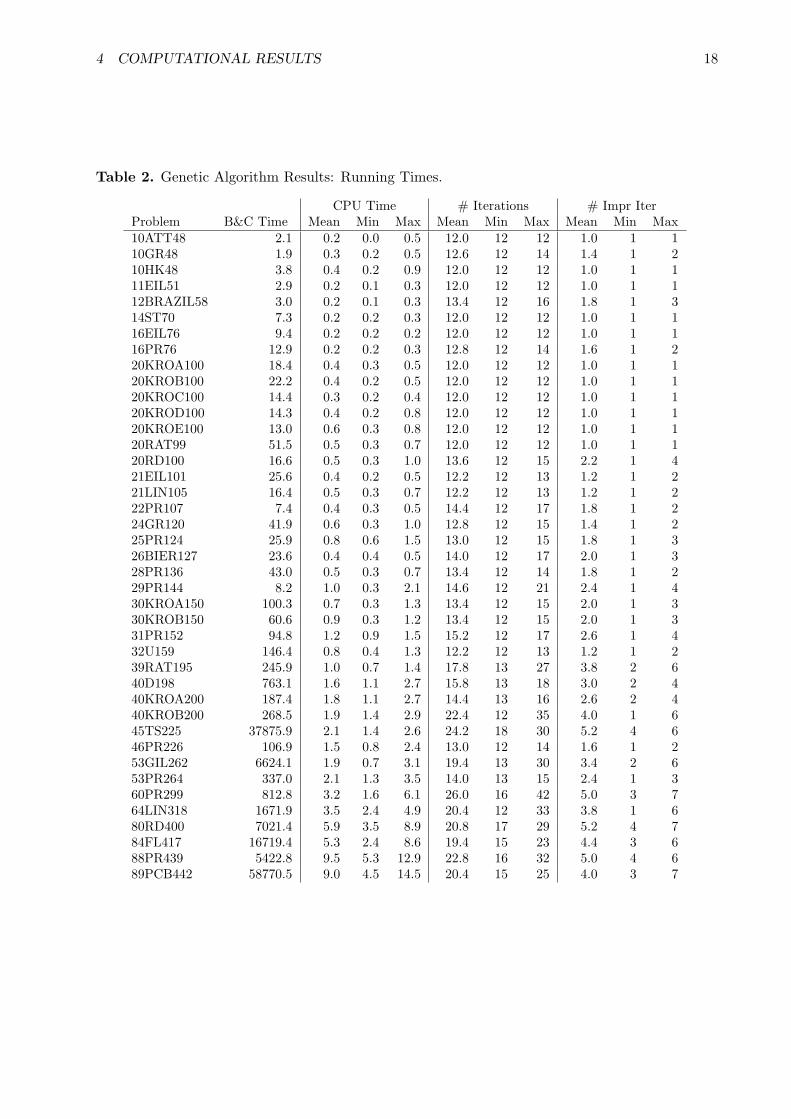
Table 2 gives information about running times for each of the trials. The columns are

as follows:

Problem: As in Table 1.CPU Time: The mean, minimum, and maximum CPU time, in seconds, for each of

the five trials of the GA.# Iterations: The mean, minimum, and maximum number of iterations before the

GA terminated.# Impr Iter: The mean, minimum, and maximum number of iterations during which

the GA found a new solution better than the current best solution (excluding thefirst iteration).

The heuristic executes extremely quickly, with a mean CPU time of less than 10

seconds for all problems and a maximum of less than 15 seconds. The GA generally

found its best solution in the first 2 or 3 iterations or so and spent most of the iterations

waiting to terminate. In general, the bulk of the running time (ranging from 65% for the

smaller problems to 95% for the larger problems) is spent in the improvement heuristic,

suggesting that a more efficient improvement method (such as Renaud and Boctor’s

G2-opt or G3-opt) may improve the speed of the GA even more.

Note that the GA seems to perform equally well for problems with modified Eu-

clidean distances (10ATT48), and explicit distances (10GR48, 10HK48, 12BRAZIL5,

4 COMPUTATIONAL RESULTS 18

Table 2. Genetic Algorithm Results: Running Times.

CPU Time # Iterations # Impr IterProblem B&C Time Mean Min Max Mean Min Max Mean Min Max10ATT48 2.1 0.2 0.0 0.5 12.0 12 12 1.0 1 110GR48 1.9 0.3 0.2 0.5 12.6 12 14 1.4 1 210HK48 3.8 0.4 0.2 0.9 12.0 12 12 1.0 1 111EIL51 2.9 0.2 0.1 0.3 12.0 12 12 1.0 1 112BRAZIL58 3.0 0.2 0.1 0.3 13.4 12 16 1.8 1 314ST70 7.3 0.2 0.2 0.3 12.0 12 12 1.0 1 116EIL76 9.4 0.2 0.2 0.2 12.0 12 12 1.0 1 116PR76 12.9 0.2 0.2 0.3 12.8 12 14 1.6 1 220KROA100 18.4 0.4 0.3 0.5 12.0 12 12 1.0 1 120KROB100 22.2 0.4 0.2 0.5 12.0 12 12 1.0 1 120KROC100 14.4 0.3 0.2 0.4 12.0 12 12 1.0 1 120KROD100 14.3 0.4 0.2 0.8 12.0 12 12 1.0 1 120KROE100 13.0 0.6 0.3 0.8 12.0 12 12 1.0 1 120RAT99 51.5 0.5 0.3 0.7 12.0 12 12 1.0 1 120RD100 16.6 0.5 0.3 1.0 13.6 12 15 2.2 1 421EIL101 25.6 0.4 0.2 0.5 12.2 12 13 1.2 1 221LIN105 16.4 0.5 0.3 0.7 12.2 12 13 1.2 1 222PR107 7.4 0.4 0.3 0.5 14.4 12 17 1.8 1 224GR120 41.9 0.6 0.3 1.0 12.8 12 15 1.4 1 225PR124 25.9 0.8 0.6 1.5 13.0 12 15 1.8 1 326BIER127 23.6 0.4 0.4 0.5 14.0 12 17 2.0 1 328PR136 43.0 0.5 0.3 0.7 13.4 12 14 1.8 1 229PR144 8.2 1.0 0.3 2.1 14.6 12 21 2.4 1 430KROA150 100.3 0.7 0.3 1.3 13.4 12 15 2.0 1 330KROB150 60.6 0.9 0.3 1.2 13.4 12 15 2.0 1 331PR152 94.8 1.2 0.9 1.5 15.2 12 17 2.6 1 432U159 146.4 0.8 0.4 1.3 12.2 12 13 1.2 1 239RAT195 245.9 1.0 0.7 1.4 17.8 13 27 3.8 2 640D198 763.1 1.6 1.1 2.7 15.8 13 18 3.0 2 440KROA200 187.4 1.8 1.1 2.7 14.4 13 16 2.6 2 440KROB200 268.5 1.9 1.4 2.9 22.4 12 35 4.0 1 645TS225 37875.9 2.1 1.4 2.6 24.2 18 30 5.2 4 646PR226 106.9 1.5 0.8 2.4 13.0 12 14 1.6 1 253GIL262 6624.1 1.9 0.7 3.1 19.4 13 30 3.4 2 653PR264 337.0 2.1 1.3 3.5 14.0 13 15 2.4 1 360PR299 812.8 3.2 1.6 6.1 26.0 16 42 5.0 3 764LIN318 1671.9 3.5 2.4 4.9 20.4 12 33 3.8 1 680RD400 7021.4 5.9 3.5 8.9 20.8 17 29 5.2 4 784FL417 16719.4 5.3 2.4 8.6 19.4 15 23 4.4 3 688PR439 5422.8 9.5 5.3 12.9 22.8 16 32 5.0 4 689PCB442 58770.5 9.0 4.5 14.5 20.4 15 25 4.0 3 7

4 COMPUTATIONAL RESULTS 19

and 24GR120) as it does for those with Euclidean distances. We were unable to test

problems with non-geographic clusters (for example, in which nodes are grouped ran-

domly) since no optimal objective values have been published for such problems.

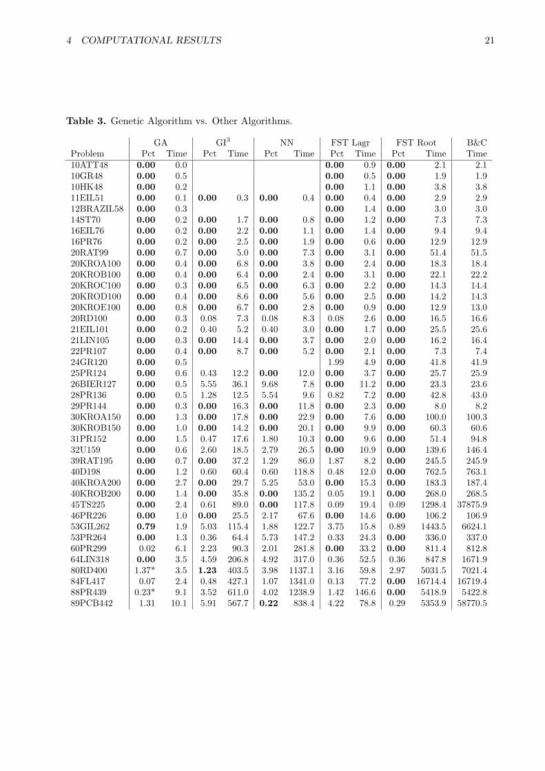
4.4 Comparison to Other Algorithms

Table 3 compares the performance of the GA with that of several other algorithms (four

heuristics and one exact algorithm) on the same TSPLIB problems. The first is the GI3

heuristic proposed by Renaud and Boctor [32]; the second is Noon’s generalized nearest

neighbor heuristic [27] combined with the improvement phase from the GI3 heuristic

(results cited in [32]). Renaud and Boctor omit the great-circle problems, as well as

several others. The heuristics labeled “FST-Lagr” and “FST-Root” in Table 3 are the

Lagrangian procedure and the root-node procedure described in [14]; these procedures

produce initial bounds at the root node of the branch-and-cut tree. Table 3 lists both

the solution quality (percent above optimal) and CPU time for all five heuristics, as

well as the solution time for the branch-and-cut procedure (an exact algorithm, not a

heuristic) in [14]. The solution value and times reported for our GA heuristic are for

the first trial (of the five trials reported in Tables 1 and 2) for each problem, so that

we are comparing a single run of our procedure with a single run of each of the others.

Minimum values for the “Pct” field in each row are marked in bold. Problems for which

the GA did not find the best solution (among all heuristics) in the first trial but did

find it in one of the other trials are indicated with an asterisk (*).

The columns are as follows:

Problem: As in Table 1.

GA: The percentage error of the solution returned in the first of five GA trials and thecorresponding CPU time (in seconds) on a Gateway Profile 4MX with Pentium IV3.2 GHz processor and 1 GB RAM.

4 COMPUTATIONAL RESULTS 20

GI3: The percentage error of the solution returned by the GI3 heuristic and the corre-sponding CPU time (in seconds) on a Sun Sparc Station LX, as reported in Table3 of [32].

NN: The percentage error of the solution returned by the NN heuristic (followed bythe improvement phase of GI3) and the corresponding CPU time (in seconds) ona Sun Sparc Station LX, as reported in Table 3 of [32].

FST-Lagr: The percentage error of the solution returned by Fischetti, Salazar-Gonzalez,and Toth’s Lagrangian heuristic and the corresponding CPU time (in seconds) onan HP 9000/720, as reported in Table I of [14].

FST-Root: The percentage error of the solution returned by Fischetti, Salazar-Gonzalez,and Toth’s root-node heuristic and the corresponding CPU time (in seconds) onan HP 9000/720, as reported in Table I of [14].

B&C: The CPU time (in seconds) of the branch-and-cut algorithm on an HP 9000/720,as reported in Table II of [14].

The first trial of the GA found the best solution among all five heuristics (allowing

for ties) in 36 out of the 41 problems tested (88%). The best solution was found in a

trial other than the first for two other problems. Two-sided paired t-tests confirm that

the objective values of the solution returned by the GA are statistically smaller than

those returned by GI3 (P = 0.002), NN (P = 0.001), and FST-Lagr (P = 0.005). The

GA also outperforms FST-Root on average, but a two-sided t-test could not prove a

significant difference (P = 0.685). (FST-Root seems to be a much slower procedure

than the GA, even allowing for differences in CPU speeds.)

A direct comparison of solution times is difficult since the procedures were coded and

tested on different machines. If we make the assumption (conservatively, we feel—see

[10]) that the machine used to test the GA is 50 times faster than the Sun Sparc Station

LX used to test GI3 and NN and 100 times faster than the HP 9000/720 used to test

FST-Lagr, FST-Root, and the branch-and-cut algorithm, our times are competitive with

those of GI3, NN, FST-Root, and branch-and-cut, and in some cases greatly outperform

them. The run times for the GA are longer than those for FST-Lagr, but the solutions

produced by the GA are at least as good as those produced by FST-Lagr for all but one

4 COMPUTATIONAL RESULTS 21

Table 3. Genetic Algorithm vs. Other Algorithms.

GA GI3 NN FST Lagr FST Root B&CProblem Pct Time Pct Time Pct Time Pct Time Pct Time Time10ATT48 0.00 0.0 0.00 0.9 0.00 2.1 2.110GR48 0.00 0.5 0.00 0.5 0.00 1.9 1.910HK48 0.00 0.2 0.00 1.1 0.00 3.8 3.811EIL51 0.00 0.1 0.00 0.3 0.00 0.4 0.00 0.4 0.00 2.9 2.912BRAZIL58 0.00 0.3 0.00 1.4 0.00 3.0 3.014ST70 0.00 0.2 0.00 1.7 0.00 0.8 0.00 1.2 0.00 7.3 7.316EIL76 0.00 0.2 0.00 2.2 0.00 1.1 0.00 1.4 0.00 9.4 9.416PR76 0.00 0.2 0.00 2.5 0.00 1.9 0.00 0.6 0.00 12.9 12.920RAT99 0.00 0.7 0.00 5.0 0.00 7.3 0.00 3.1 0.00 51.4 51.520KROA100 0.00 0.4 0.00 6.8 0.00 3.8 0.00 2.4 0.00 18.3 18.420KROB100 0.00 0.4 0.00 6.4 0.00 2.4 0.00 3.1 0.00 22.1 22.220KROC100 0.00 0.3 0.00 6.5 0.00 6.3 0.00 2.2 0.00 14.3 14.420KROD100 0.00 0.4 0.00 8.6 0.00 5.6 0.00 2.5 0.00 14.2 14.320KROE100 0.00 0.8 0.00 6.7 0.00 2.8 0.00 0.9 0.00 12.9 13.020RD100 0.00 0.3 0.08 7.3 0.08 8.3 0.08 2.6 0.00 16.5 16.621EIL101 0.00 0.2 0.40 5.2 0.40 3.0 0.00 1.7 0.00 25.5 25.621LIN105 0.00 0.3 0.00 14.4 0.00 3.7 0.00 2.0 0.00 16.2 16.422PR107 0.00 0.4 0.00 8.7 0.00 5.2 0.00 2.1 0.00 7.3 7.424GR120 0.00 0.5 1.99 4.9 0.00 41.8 41.925PR124 0.00 0.6 0.43 12.2 0.00 12.0 0.00 3.7 0.00 25.7 25.926BIER127 0.00 0.5 5.55 36.1 9.68 7.8 0.00 11.2 0.00 23.3 23.628PR136 0.00 0.5 1.28 12.5 5.54 9.6 0.82 7.2 0.00 42.8 43.029PR144 0.00 0.3 0.00 16.3 0.00 11.8 0.00 2.3 0.00 8.0 8.230KROA150 0.00 1.3 0.00 17.8 0.00 22.9 0.00 7.6 0.00 100.0 100.330KROB150 0.00 1.0 0.00 14.2 0.00 20.1 0.00 9.9 0.00 60.3 60.631PR152 0.00 1.5 0.47 17.6 1.80 10.3 0.00 9.6 0.00 51.4 94.832U159 0.00 0.6 2.60 18.5 2.79 26.5 0.00 10.9 0.00 139.6 146.439RAT195 0.00 0.7 0.00 37.2 1.29 86.0 1.87 8.2 0.00 245.5 245.940D198 0.00 1.2 0.60 60.4 0.60 118.8 0.48 12.0 0.00 762.5 763.140KROA200 0.00 2.7 0.00 29.7 5.25 53.0 0.00 15.3 0.00 183.3 187.440KROB200 0.00 1.4 0.00 35.8 0.00 135.2 0.05 19.1 0.00 268.0 268.545TS225 0.00 2.4 0.61 89.0 0.00 117.8 0.09 19.4 0.09 1298.4 37875.946PR226 0.00 1.0 0.00 25.5 2.17 67.6 0.00 14.6 0.00 106.2 106.953GIL262 0.79 1.9 5.03 115.4 1.88 122.7 3.75 15.8 0.89 1443.5 6624.153PR264 0.00 1.3 0.36 64.4 5.73 147.2 0.33 24.3 0.00 336.0 337.060PR299 0.02 6.1 2.23 90.3 2.01 281.8 0.00 33.2 0.00 811.4 812.864LIN318 0.00 3.5 4.59 206.8 4.92 317.0 0.36 52.5 0.36 847.8 1671.980RD400 1.37* 3.5 1.23 403.5 3.98 1137.1 3.16 59.8 2.97 5031.5 7021.484FL417 0.07 2.4 0.48 427.1 1.07 1341.0 0.13 77.2 0.00 16714.4 16719.488PR439 0.23* 9.1 3.52 611.0 4.02 1238.9 1.42 146.6 0.00 5418.9 5422.889PCB442 1.31 10.1 5.91 567.7 0.22 838.4 4.22 78.8 0.29 5353.9 58770.5

4 COMPUTATIONAL RESULTS 22

problem. Aside from solution quality and run time, FST-Lagr and the GA each have

their advantages: FST-Lagr provides a lower bound on the optimal objective value,

while the GA is simpler to code and can easily be modified to incorporate alternate

objective functions and constraints.

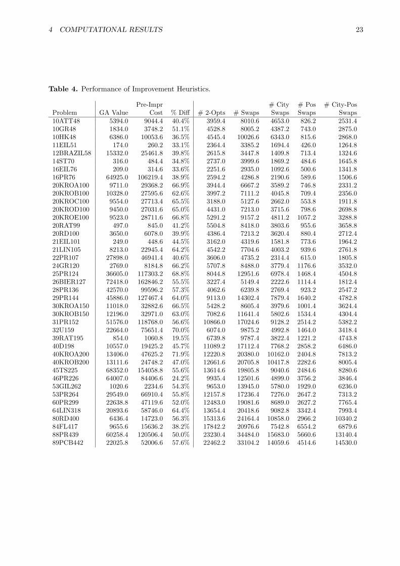
4.5 Contribution of Algorithm Features

In this section we examine the relative contribution of each of the features of the GA to

the heuristic’s overall performance. Table 4 reports the mean cost of the best solution

found (out of 5 trials) both before and after the improvement heuristic was performed.

It also reports the number of 2-opts and swaps, as well as the breakdown of swaps by

type: changing which city from a cluster is included on the tour but not the position

of the city, changing the position of a city but not which city is included, and changing

both. The columns are as follows:

Problem: As in Table 1.GA Value: The mean objective value (out of 5 trials) returned by the GA, replicated

from Table 1.Pre-Impr Cost: The mean pre-improvement cost (out of 5 trials) of the best solu-

tion found by the GA. (That is, the mean pre-improvement cost of the 5 post-improvement solutions considered in the “GA Value” column.)

% Diff: The percentage difference between “GA Value” and “Pre-Impr Cost.”# 2-Opts: The mean number of 2-opts (out of 5 trials) performed during the GA’s

execution.# Swaps: The mean number of swaps (out of 5 trials) performed during the GA’s

execution.# City Swaps: The mean number of swaps (out of 5 trials) that involved changing a

cluster’s included city (but not the position of the cluster on the tour).# Pos Swaps: The mean number of swaps (out of 5 trials) that involved changing the

position of a cluster on the tour (but not the cluster’s included city).# City-Pos Swaps: The mean number of swaps (out of 5 trials) that involved chang-

ing both a cluster’s included city and its position on the tour.

Clearly, the improvement heuristics play a large role in the overall performance of

the GA. The quality of the solution returned by the GA is due in large part to the

4 COMPUTATIONAL RESULTS 23

Table 4. Performance of Improvement Heuristics.

Pre-Impr # City # Pos # City-PosProblem GA Value Cost % Diff # 2-Opts # Swaps Swaps Swaps Swaps10ATT48 5394.0 9044.4 40.4% 3959.4 8010.6 4653.0 826.2 2531.410GR48 1834.0 3748.2 51.1% 4528.8 8005.2 4387.2 743.0 2875.010HK48 6386.0 10053.6 36.5% 4545.4 10026.6 6343.0 815.6 2868.011EIL51 174.0 260.2 33.1% 2364.4 3385.2 1694.4 426.0 1264.812BRAZIL58 15332.0 25461.8 39.8% 2615.8 3447.8 1409.8 713.4 1324.614ST70 316.0 484.4 34.8% 2737.0 3999.6 1869.2 484.6 1645.816EIL76 209.0 314.6 33.6% 2251.6 2935.0 1092.6 500.6 1341.816PR76 64925.0 106219.4 38.9% 2594.2 4286.8 2190.6 589.6 1506.620KROA100 9711.0 29368.2 66.9% 3944.4 6667.2 3589.2 746.8 2331.220KROB100 10328.0 27595.6 62.6% 3997.2 7111.2 4045.8 709.4 2356.020KROC100 9554.0 27713.4 65.5% 3188.0 5127.6 2662.0 553.8 1911.820KROD100 9450.0 27031.6 65.0% 4431.0 7213.0 3715.6 798.6 2698.820KROE100 9523.0 28711.6 66.8% 5291.2 9157.2 4811.2 1057.2 3288.820RAT99 497.0 845.0 41.2% 5504.8 8418.0 3803.6 955.6 3658.820RD100 3650.0 6078.0 39.9% 4386.4 7213.2 3620.4 880.4 2712.421EIL101 249.0 448.6 44.5% 3162.0 4319.6 1581.8 773.6 1964.221LIN105 8213.0 22945.4 64.2% 4542.2 7704.6 4003.2 939.6 2761.822PR107 27898.0 46941.4 40.6% 3606.0 4735.2 2314.4 615.0 1805.824GR120 2769.0 8184.8 66.2% 5707.8 8488.0 3779.4 1176.6 3532.025PR124 36605.0 117303.2 68.8% 8044.8 12951.6 6978.4 1468.4 4504.826BIER127 72418.0 162846.2 55.5% 3227.4 5149.4 2222.6 1114.4 1812.428PR136 42570.0 99596.2 57.3% 4062.6 6239.8 2769.4 923.2 2547.229PR144 45886.0 127467.4 64.0% 9113.0 14302.4 7879.4 1640.2 4782.830KROA150 11018.0 32882.6 66.5% 5428.2 8605.4 3979.6 1001.4 3624.430KROB150 12196.0 32971.0 63.0% 7082.6 11641.4 5802.6 1534.4 4304.431PR152 51576.0 118768.0 56.6% 10866.0 17024.6 9128.2 2514.2 5382.232U159 22664.0 75651.4 70.0% 6074.0 9875.2 4992.8 1464.0 3418.439RAT195 854.0 1060.8 19.5% 6739.8 9787.4 3822.4 1221.2 4743.840D198 10557.0 19425.2 45.7% 11089.2 17112.4 7768.2 2858.2 6486.040KROA200 13406.0 47625.2 71.9% 12220.8 20380.0 10162.0 2404.8 7813.240KROB200 13111.6 24748.2 47.0% 12661.6 20705.8 10417.8 2282.6 8005.445TS225 68352.0 154058.8 55.6% 13614.6 19805.8 9040.6 2484.6 8280.646PR226 64007.0 84406.6 24.2% 9935.4 12501.6 4899.0 3756.2 3846.453GIL262 1020.6 2234.6 54.3% 9653.0 13945.0 5780.0 1929.0 6236.053PR264 29549.0 66910.4 55.8% 12157.8 17236.4 7276.0 2647.2 7313.260PR299 22638.8 47119.6 52.0% 12483.0 19081.6 8689.0 2627.2 7765.464LIN318 20893.6 58746.0 64.4% 13654.4 20418.6 9082.8 3342.4 7993.480RD400 6436.4 14723.0 56.3% 15313.6 24164.4 10858.0 2966.2 10340.284FL417 9655.6 15636.2 38.2% 17842.2 20976.6 7542.8 6554.2 6879.688PR439 60258.4 120506.4 50.0% 23230.4 34484.0 15683.0 5660.6 13140.489PCB442 22025.8 52006.6 57.6% 22462.2 33104.2 14059.6 4514.6 14530.0

4 COMPUTATIONAL RESULTS 24

improvement heuristics, and each heuristic is performed many times during the GA’s

execution. Moreover, each type of heuristic (2-opt and all three types of swaps) is used

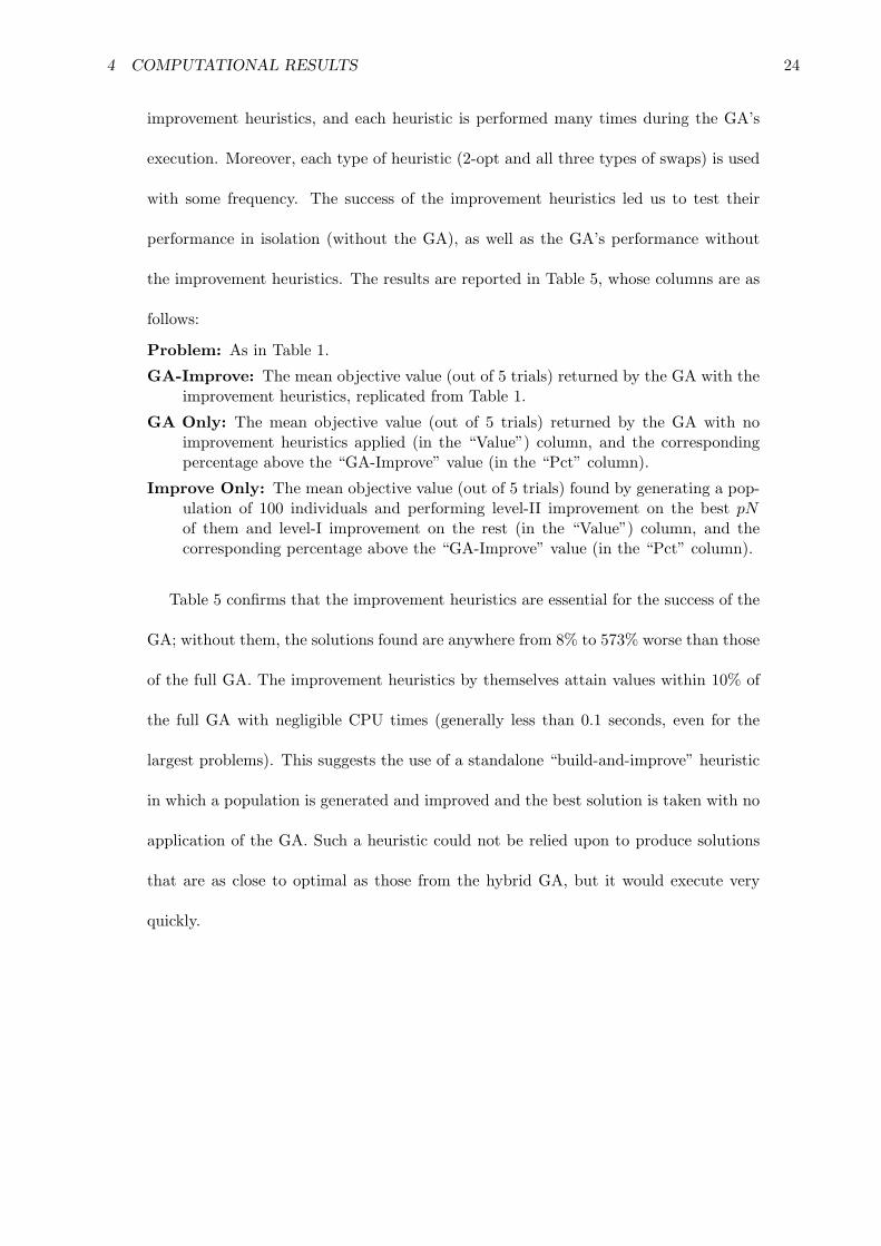
with some frequency. The success of the improvement heuristics led us to test their

performance in isolation (without the GA), as well as the GA’s performance without

the improvement heuristics. The results are reported in Table 5, whose columns are as

follows:

Problem: As in Table 1.

GA-Improve: The mean objective value (out of 5 trials) returned by the GA with theimprovement heuristics, replicated from Table 1.

GA Only: The mean objective value (out of 5 trials) returned by the GA with noimprovement heuristics applied (in the “Value”) column, and the correspondingpercentage above the “GA-Improve” value (in the “Pct” column).

Improve Only: The mean objective value (out of 5 trials) found by generating a pop-ulation of 100 individuals and performing level-II improvement on the best pNof them and level-I improvement on the rest (in the “Value”) column, and thecorresponding percentage above the “GA-Improve” value (in the “Pct” column).

Table 5 confirms that the improvement heuristics are essential for the success of the

GA; without them, the solutions found are anywhere from 8% to 573% worse than those

of the full GA. The improvement heuristics by themselves attain values within 10% of

the full GA with negligible CPU times (generally less than 0.1 seconds, even for the

largest problems). This suggests the use of a standalone “build-and-improve” heuristic

in which a population is generated and improved and the best solution is taken with no

application of the GA. Such a heuristic could not be relied upon to produce solutions

that are as close to optimal as those from the hybrid GA, but it would execute very

quickly.

4 COMPUTATIONAL RESULTS 25

Table 5. GA-Only and Improve-Only Results.

GA Only Improve OnlyProblem GA-Improve Value Pct Value Pct10ATT48 5394.0 6313.4 17.04 5396.0 0.0410GR48 1834.0 2079.4 13.38 1861.4 1.4910HK48 6386.0 6921.6 8.39 6386.0 0.0011EIL51 174.0 227.4 30.69 175.0 0.5712BRAZIL58 15332.0 19124.0 24.73 15458.6 0.8314ST70 316.0 450.8 42.66 318.4 0.7616EIL76 209.0 352.0 68.42 213.4 2.1116PR76 64925.0 85385.2 31.51 65315.6 0.6020KROA100 9711.0 20191.0 107.92 9711.8 0.0120KROB100 10328.0 18537.4 79.49 10362.0 0.3320KROC100 9554.0 17871.6 87.06 9554.0 0.0020KROD100 9450.0 18477.0 95.52 9484.2 0.3620KROE100 9523.0 19787.6 107.79 9644.8 1.2820RAT99 497.0 1090.0 119.32 506.0 1.8120RD100 3650.0 7353.4 101.46 3718.4 1.8721EIL101 249.0 526.4 111.41 249.6 0.2421LIN105 8213.0 14559.4 77.27 8241.8 0.3522PR107 27898.0 57724.6 106.91 27930.2 0.1224GR120 2769.0 5628.4 103.26 2866.6 3.5225PR124 36605.0 82713.0 125.96 36835.4 0.6326BIER127 72418.0 154703.2 113.63 76666.2 5.8728PR136 42570.0 112674.6 164.68 45421.4 6.7029PR144 45886.0 94969.2 106.97 46543.0 1.4330KROA150 11018.0 31199.2 183.17 11029.0 0.1030KROB150 12196.0 34685.2 184.40 12549.0 2.8931PR152 51576.0 118813.4 130.37 52772.8 2.3232U159 22664.0 59099.2 160.76 22889.2 0.9939RAT195 854.0 2844.2 233.04 901.0 5.5040D198 10557.0 26453.0 150.57 10704.0 1.3940KROA200 13406.0 46866.4 249.59 14209.4 5.9940KROB200 13111.6 47303.2 260.77 13543.0 3.2945TS225 68352.0 229495.2 235.75 70775.4 3.5546PR226 64007.0 263699.0 311.98 66250.6 3.5153GIL262 1020.6 4233.6 314.81 1091.4 6.9453PR264 29549.0 145789.4 393.38 30603.6 3.5760PR299 22638.8 110977.8 390.21 24520.0 8.3164LIN318 20893.6 94469.2 352.14 22272.8 6.6080RD400 6436.4 34502.2 436.05 6789.4 5.4884FL417 9655.6 65025.6 573.45 10168.4 5.3188PR439 60258.4 364282.4 504.53 66364.0 10.1389PCB442 22025.8 131711.8 497.99 23586.0 7.08

5 CONCLUSIONS AND FUTURE RESEARCH DIRECTIONS 26

5 Conclusions and Future Research Directions

This paper presents a heuristic to solve the generalized traveling salesman problem. The

procedure incorporates a local tour improvement heuristic into a random-key genetic

algorithm. The algorithm performed quite well when tested on a set of 41 standard

problems with known optimal objective values, finding the optimal solution in the ma-

jority of cases. Computation times were small (under 15 seconds), and the GA returned

fairly consistent results among trials.

Our GA performs competitively with other heuristics that have been published, both

in solution quality and computation time. Moreover, our heuristic has two main advan-

tages over others. First, it is quite simple to implement. Second, it can be extended

easily to incorporate alternate objective functions and constraints. For example, one

could allow ri ≥ 1 nodes to be required for set Vi. Thus, we might require the tour to

visit two nodes from V1, five nodes from V2, and so on. This would require ri genes

for set Vi. Crossover would operate on all ri genes as a group, rather than individu-

ally, to maintain feasibility. Or, by including demand-weighted “medial” distances in

the objective function, one could solve the Median Tour Problem [8, 34]. Similarly,

by including secondary tours that connect the customers in each cluster to the main

tour one can solve the Traveling Circus Problem [34]; this problem would require fur-

ther modifications to the encoding scheme, but it is particularly appealing because it

has as a special case the vehicle routing problem (VRP) and the multi-depot VRP. Of

course, the success of our algorithm for the classical GTSP does not imply its success

for these variations; further computational tests would need to be performed to judge

its applicability to these problems.

REFERENCES 27

References

[1] J. T. Alander, editor. Proceedings of the First Nordic Workshop on Genetic Al-

gorithms and their Applications (1NWGA). January 9-12, 1995, Vaasa Yliopiston

Julkaisuja, Vaasa, 1995.

[2] W. Banzhaf, J. Daida, A. E. Eiben, M. H. Garzon, V. Honavar, M. Jakiela, and

R. E. Smith, editors. Proceedings of the Genetic and Evolutionary Computation

Conference. Orlando, FL, July 13-17, 1999, Morgan Kaufmann, San Mateo, CA,

1999.

[3] J. C. Bean. Genetic algorithms and random keys for sequencing and optimization.

ORSA Journal on Computing, 6:154–160, 1994.

[4] R. K. Belew and L. B. Booker, editors. Proceedings of the Fourth International

Conference on Genetic Algorithms. University of California, San Diego, July 13-

16, 1991, Morgan Kaufmann, San Mateo, CA, 1991.

[5] D. Ben-Arieh, G. Gutin, M. Penn, A. Yeo, and A. Zverovitch. Process planning for

rotational parts using the generalized traveling salesman problem. International

Journal of Production Research, 41(11):2581–2596, 2003.

[6] D. Ben-Arieh, G. Gutin, M. Penn, A. Yeo, and A. Zverovitch. Transformations of

generalized atsp into atsp. Operations Research Letters, 31:357–365, 2003.

[7] A. G. Chentsov and L. N. Korotayeva. The dynamic programming method in the

generalized traveling salesman problem. Mathematical and Computer Modelling,

25(1):93–105, 1997.

[8] J. R. Current and D. A. Schilling. The median tour and maximal covering tour

problems: Formulations and heuristics. European Journal of Operational Research,

REFERENCES 28

73:114–126, 1994.

[9] V. Dimitrijevic and Z. Saric. An efficient transformation of the generalized traveling

salesman problem into the traveling salesman problem on digraphs. Information

Sciences, 102(1-4):105–110, 1997.

[10] J. J. Dongarra. Performance of various computers using standard linear equations

software. Technical Report CS-89-85, Computer Science Department, University

of Tennessee, 2004.

[11] M. Dror and M. Haouari. Generalized steiner problems and other variants. Journal

of Combinatorial Optimization, 4(4):415–436, 2000.

[12] M. Dror and A. Langevin. A generalized traveling salesman problem approach to

the directed clustered rural postman problem. Transportation Science, 31(2):187–

192, 1997.

[13] M. Fischetti, J. J. Salazar-Gonzalez, and P. Toth. The symmetrical generalized

traveling salesman polytope. Networks, 26(2):113–123, 1995.

[14] M. Fischetti, J. J. Salazar-Gonzalez, and P. Toth. A branch-and-cut algorithm

for the symmetric generalized traveling salesman problem. Operations Research,

45(3):378–394, 1997.

[15] N. Garg, G. Konjevod, and R. Ravi. A polylogarithmic approximation algorithm

for the group steiner tree problem. Journal of Algorithms, 37(1):66–84, 2000.

[16] A. Henry-Labordere. The record balancing problem - a dynamic programming solu-

tion of a generalized traveling salesman problem. Revue Francaise D Informatique

De Recherche Operationnelle, 3(NB2):43–49, 1969.

REFERENCES 29

[17] J. R. Koza, D. E. Goldberg, D. B. Fogel, and R. L. Riolo, editors. Genetic Pro-

gramming: Proceedings of the First Annual Conference. Stanford University, July

28-31, 1996, MIT Press, Cambridge, 1996.

[18] V. M. Kureichick, V. V. Miagkikh, and A. P. Topchy. Genetic algorithm for solu-

tion of the traveling salesman problem with new features against premature conver-

gence. Working paper, Taganrog State University of Radio-Engineering, Taganrog,

Russia, 1996.

[19] G. Laporte, A. Asef-Vaziri, and C. Sriskandarajah. Some applications of the gen-

eralized travelling salesman problem. Journal of the Operational Research Society,

47(12):1461–1467, 1996.

[20] G. Laporte, H. Mercure, and Y. Nobert. Finding the shortest Hamiltonian circuit

through n clusters: A Lagrangian approach. Congressus Numerantium, 48:277–290,

1985.

[21] G. Laporte, H. Mercure, and Y. Nobert. Generalized traveling salesman problem

through n-sets of nodes - the asymmetrical case. Discrete Applied Mathematics,

18(2):185–197, 1987.

[22] G. Laporte and Y. Nobert. Generalized traveling salesman problem through n-sets

of nodes - an integer programming approach. INFOR, 21(1):61–75, 1983.

[23] G. Laporte and F. Semet. Computational evaluation of a transformation procedure

for the symmetric generalized traveling salesman problem. INFOR, 37(2):114–120,

1999.

[24] D. Levine. Application of a hybrid genetic algorithm to airline crew scheduling.

Computers & Operations Research, 23(6):547–558, 1996.

REFERENCES 30

[25] Y. N. Lien, E. Ma, and B. W. S. Wah. Transformation of the generalized traveling-

salesman problem into the standard traveling-salesman problem. Information Sci-

ences, 74(1-2):177–189, 1993.

[26] K. F. Man, K. S. Tang, and S. Kwong. Genetic Algorithms: Concepts and Designs.

Springer, New York, 1999.

[27] C. E. Noon. The Generalized Traveling Salesman Problem. PhD thesis, University

of Michigan, 1988.

[28] C. E. Noon and J. C. Bean. A lagrangian based approach for the asymmetric

generalized traveling salesman problem. Operations Research, 39(4):623–632, 1991.

[29] C. E. Noon and J. C. Bean. An efficient transformation of the generalized traveling

salesman problem. INFOR, 31(1):39–44, 1993.

[30] J. E. Rawlins, Gregory, editor. Foundations of Genetic Algorithms. Morgan Kauf-

mann, San Mateo, CA, 1991.

[31] G. Reinelt. TSPLIB—a traveling salesman problem library. ORSA Journal on

Computing, 4:134–143, 1996.

[32] J. Renaud and F. F. Boctor. An efficient composite heuristic for the symmetric

generalized traveling salesman problem. European Journal of Operational Research,

108(3):571–584, 1998.

[33] J. Renaud, F. F. Boctor, and G. Laporte. A fast composite heuristic for the

symmetric traveling salesman problem. INFORMS Journal on Computing, 4:134–

143, 1996.

[34] C. S. Revelle and G. Laporte. The plant location problem: New models and

research prospects. Operations Research, 44(6):864–874, 1996.

REFERENCES 31

[35] J. P. Saskena. Mathematical model of scheduling clients through welfare agencies.

Journal of the Canadian Operational Research Society, 8:185–200, 1970.

[36] P. Slavık. On the approximation of the generalized traveling salesman problem.

Working paper, Department of Computer Science, SUNY-Buffalo, 1997.

[37] W. M. Spears and K. A. DeJong. On the virtues of parameterized uniform

crossover. In Proceedings of the Fourth International Conference on Genetic Algo-

rithms, pages 230–236, 1991.

[38] S. S. Srivastava, S. Kumar, R. C. Garg, and P. Sen. Generalized traveling salesman

problem through n sets of nodes. Journal of the Canadian Operational Research

Society, 7:97–101, 1970.

[39] L. D. Whitley, editor. Foundations of Genetic Algorithms 2. Morgan Kaufmann,

San Mateo, CA, 1993.

[40] G. Winter, J. Periaux, M. Galan, and P. Cuesta, editors. Genetic Algorithms in

Engineering and Computer Science. Wiley, New York, 1995.

[41] A. M. S. Zalzala and P. J. Fleming, editors. Genetic Algorithms in Engineering

Systems. The Institution of Electrical Engineers, London, 1997.