Copula based generalized additive models with

non-random sample selection

Ma lgorzata WojtysCentre for Mathematical Sciences

Plymouth University

Drake Circus, Plymouth PL4 8AA, U.K.

Giampiero MarraDepartment of Statistical Science

University College London

Gower Street, London WC1E 6BT, U.K.

Abstract

Non-random sample selection is a commonplace amongst many empirical studies

and it appears when an output variable of interest is available only for a restricted

non-random sub-sample of data. We introduce an extension of the generalized additive

model which accounts for non-random sample selection by using a selection equation.

The proposed approach allows for different distributions of the outcome variable, vari-

ous dependence structures between the (outcome and selection) equations through the

use of copulae, and nonparametric effects on the responses. Parameter estimation is

carried out within a penalized likelihood and simultaneous equation framework. We es-

tablish asymptotic theory for the proposed penalized spline estimators, which extends

the recent theoretical results for penalized splines in generalized additive models, such

as those by Kauermann et al. (2009) and Yoshida & Naito (2014). The empirical

effectiveness of the approach is demonstrated through a simulation study.

Key Words: copula, generalized additive model, non-random sample selection,

penalized regression spline, selection bias, simultaneous equation estimation.

1 Introduction

Non-random sample selection arises when an output variable of interest is available only for

a restricted non-random sub-sample of the data. This often occurs in sociological, medical

and economic studies where individuals systematically select themselves into (or out of) the

sample (see, e.g., Guo & Fraser (2014), chapter 4, Lennox et al. (2012), Vella (1998), Collier

& Mahoney (1996) and references therein). If the aim is to model an outcome of interest in

the entire population and the link between its availability in the sub-sample and its observed

values is through factors which can not be accounted for then any analysis based on the

1

arX

iv:1

508.

0407

0v1

[m

ath.

ST]

17

Aug

201

5

available sub-sample only will yield erroneous model structures and biased conclusions as

the resulting inference may not extend to the unobserved group of observations. Sample

selection models allow us to use the entire sample whether or not observations on the output

variable were generated. In its classical form, it consists of two equations which model the

probability of inclusion in the sample and the outcome variable through a set of available

predictors, and of a joint bivariate distribution linking the two equations.

The sample selection model was first introduced by Gronau (1974), Lewis (1974) and

Heckman (1974), in the context of estimating the number of working hours and wage rates of

married women, some of whom did not work. Heckman (1976) formulated a unified approach

to estimating this model as a simultaneous equation system. In the classical version, the

error terms of the two equations are assumed to follow a bivariate normal distribution in

which non-zero correlation indicates the presence of non-random sample selection. Heckman

(1979) then translated the issue of sample selection into an omitted variable problem and

proposed a simple and easy to implement estimation method known as two-step procedure.

However, the method was proved to strongly rely on the assumption of normality and thus

has been criticized for its lack of robustness to distributional misspecification and outliers

(e.g., Paarsch, 1984; Little & Rubin, 1987; Zuehlke & Zeman, 1991; Zhelonkin, 2013).

Various modifications and generalizations of the classical sample selection model have

been proposed in the literature and we mention some of them. A non-parametric approach,

which lifts the normality assumption, can be found in Das et al. (2003). Here a two-stage

Heckman’s method is adopted and a linear regression with the Heckman’s selection correc-

tion is replaced with series expansions. Non-parametric methods are also considered in Lee

(2008) and Chen & Zhou (2010). Semi-parametric techniques in a two-step scenario, similar

to that in Das et al. (2003), are given in Ahn & Powell (1993), Newey (1999) and Pow-

ell (1994). Other semi-parametric approaches can be found in Gallant & Nychka (1987),

Powell et al. (1989), Lee (1994a), Lee (1994b), Andrews & Schafgans (1998) and Newey

(2009). In the Bayesian framework, Chib et al. (2009) deal with non-linear covariate effects

using Markov chain Monte Carlo simulation techniques and simultaneous equation systems.

Wiesenfarth & Kneib (2010) further extend this approach by introducing a Bayesian algo-

rithm based on low rank penalized B-splines for non-linear and varying-coefficient effects and

Markov random-field priors for spatial effects. A frequentist counterpart of these Bayesian

methods is discussed in Marra & Radice (2013b) in the context of binary outcomes and

Marra & Radice (2013a) for the continuous outcome case. Zhelonkin et al. (2012) intro-

duce a procedure for robustifying the Heckman’s two stage estimator by using M-estimators

of Mallows’ type for both stages. Marchenko & Genton (2012) and Ding (2014) consider

a bivariate Student-t distribution for the model’s errors as a way of tackling heavy-tailed

data. Several authors proposed specific copula functions to model the joint distribution

2

of the selection and outcome equations; see, e.g., Prieger (2002) who employes an FGM

bivariate copula or Lee (1983). In the context of non-random sample selection, a more gen-

eral copula approach, with a focus on Archimedean copulae, can be found in Smith (2003).

This stream of research is continued in Hasebe & Vijverberg (2012) and Schwiebert (2013).

As emphasized by Genius & Strazzera (2008), copulae allow for the use of non-Gaussian

distributions and has the additional benefit of making it possible to specify the marginal

distributions independently of the dependence structure linking them. Importantly, while

the copula approach is still fully parametric, it is typically computationally more feasible

than non/semi-parametric approaches and it still allows the user to assess the sensitivity of

results to different modeling assumptions.

The aim of this paper is to introduce a generalized additive model (GAM) which accounts

for non-random sample selection. Thus, the classical GAM is extended by introducing an

extra equation which models the selection process. The selection and outcome equations

are linked by a joint probability distribution which is expressed in terms of a copula. Us-

ing different copulae allows us to capture different types of dependence while keeping the

marginal distributions of the responses fixed. This approach is flexible and numerically

tractable at the same time. Secondly, we make a step towards greater flexibility in modeling

the relationship between predictors and responses by using a semiparametric approach in

place of commonly used parametric formulae, thus capturing possibly complex non-linear

relationships. We use penalized regression splines to approximate these relationships and

employ a penalized likelihood and simultaneous equation estimation framework as presented

in Marra & Radice (2013a), for instance. Penalized splines were introduced in O’Sullivan

(1986) and Eilers & Marx (1996) and practical aspects of their use received much attention

ever since; see Ruppert et al. (2003) and Wood (2006). At the same time, the asymptotic

theory for penalized spline estimators is relatively new and mainly focuses on models with

one continuous predictor (e.g., Hall & Opsomer, 2005; Claeskens et al., 2009; Wang et al.,

2011). In the GAM context, the asymptotic normality of the penalized spline estimator

has been proved by Kauermann et al. (2009) and recently extended by Yoshida & Naito

(2014) to the case of any fixed number of predictors. This paper discusses the asymptotic

properties of the penalized spline estimator of the proposed model. The asymptotic rate

of the mean squared error of the linear predictor for the regression equation of interest is

derived, which also allows us to derive its asymptotic bias and variance as well as its ap-

proximate distribution. The theoretical results are obtained for a general case of any fixed

number of predictors and when the spline basis increases with the sample size. We show

that even though the model structure is more complex than that of a classical GAM, the

asymptotic properties of penalized spline estimators are still valid. Thus, the results extend

the theoretical foundation of GAMs established so far.

3

The paper is organized as follows. Section 2 briefly describes the classical sample selection

model as well as Heckman’s estimation procedure. Section 3 introduces a generalized sample

selection model based on GAMs. Section 4 succinctly describes the estimation approach

which is based on a penalized likelihood and simultaneous equation framework. In Section

5, the asymptotic properties of the proposed penalized spline estimator are established. The

finite-sample performance of the approach is investigated in Section 6. Section 7 discusses

some extensions.

2 Classical sample selection model

The classical sample selection model introduced by Heckman (1974) and Heckman (1979) is

defined by the system of the following equations

Y ∗1i = x(1)i β1 + ε1i, (1)

Y ∗2i = x(2)i β2 + ε2i, (2)

Y1i = 1(Y ∗1i > 0), (3)

Y2i = Y ∗2iY1i , (4)

for i = 1, . . . , n, where Y ∗1i and Y ∗2i are unobserved latent variables and only values of Y1i and

Y2i are observed. The symbol 1(·) denotes throughout an indicator function. Equation (1) is

the so-called selection equation determining whether the observation of Y ∗2i is generated, and

equation (2) is the output equation of primary interest. Row vectors x(1) = (x(1)1 , . . . , x

(1)D1

) ∈RD1 and x(2) = (x

(2)1 , . . . , x

(2)D2

) ∈ RD2 contain predictors’ values and are observed for the

entire sample whereas β1 ∈ Rp and β2 ∈ Rq are unknown parameter vectors. The classical

sample selection model assumes that the error terms (ε1i, ε2i) follow the bivariate normal

distribution [ε1i

ε2i

]∼ N

([0

0

],

[1 ρσ

ρσ σ2

]),

for i = 1, . . . , n. The variance of ε1i is assumed to be equal to 1 for the usual identification

reason. The normality of ε1i implies that the selection equation represents a probit regression

expressed in terms of a latent variable. The assumption of bivariate normality of error terms

has been commonly used since. It implies that the log-likelihood of model (1)-(4) can be

4

expressed as (cf. Amemiya (1985) and eq. (10.7.3) therein)

`(β1,β2, σ, ρ|Y11, . . . , Y1n, Y21, . . . , Y2n) =n∑i=1

{(1− Y1i) log

(1− Φ(x

(1)i β1)

)+Y1i

[log Φ

(x

(1)i β1 + ρ

σ(Y2i − x

(2)i β2)√

1− ρ2

)+ log φ

(Y2i − x

(2)i β2

σ

)− log σ

]},

where Φ(·) and φ(·) denote the standard normal distribution function and density, respec-

tively. Under the model assumptions, maximization of the above function, referred to as

full-information maximum likelihood, results in consistent estimators of the parameters β1,

β2, σ and ρ but until recently was computationally cumbersome. As a consequence Heck-

man (1979) proposed a two-step procedure, also known as limited-information maximum

likelihood method. It is based on the fact that under the assumption of normality of the

error terms the following equality holds

E (ε2i|Y ∗1i > 0) = σρξ(x

(1)i β1

),

where ξ(u) = φ(u)Φ(u)

is the so-called inverse Mills ratio. Thus the conditional expectation of

the outcome variable given that its value is observed equals

E (Y ∗2i|Y ∗1i > 0) = x(2)i β2 + σρξ

(x

(1)i β1

).

In the first step of Heckman’s procedure, probit model (1) is fitted in order to obtain an

estimator of β1 and hence an estimator ξi = ξ(x

(1)i β1

)of ξ

(x

(1)i β1

). In the second step

the following regression equation is estimated through the ordinary least squares method

Y2i = x(2)i β2 + γξi + ε2i, i ∈ {j : Y ∗1j > 0},

using the selected sub-sample only, where ξi is an added variable and γ = σρ is the cor-

responding unknown parameter. After obtaining estimators β2 and γ, parameter σ can be

estimated as σ =(n−1s

∑ˆε2

2i + n−1s

∑ξi

(ξi + x

(1)i β1

))1/2

where ns is the size of the sub-

sample, i.e. the cardinality of {j : Y ∗1j > 0} (see, for instance, Toomet & Henningsen (2008)).

Thus the estimator of the correlation coefficient ρ is defined as ρ = γ/σ.

Although the inverse Mills ratio ξ(u) is known to be nonlinear, in practice it often turns

out to be approximately linear for most values in the u range. This may lead to identification

issues if both equations include the same set of predictors (Puhani, 2000, p. 57). Thus, an

exclusion restriction, which requires the availability of at least one predictor which is related

to selection process but that has no direct effect on the outcome, has to be used in empirical

5

applications. As mentioned in the introduction, Heckman’s model received a number of

criticisms due to its lack of robustness to departures from the model assumptions (see,

e.g., Paarsch, 1984; Little & Rubin, 1987; Zuehlke & Zeman, 1991; Zhelonkin, 2013, and

references therein).

3 Generalized additive sample selection model

We structure the proposed sample selection model in the following way. We first assume that

the outcome variable of interest can be described by a generalized additive model (Hastie

& Tibshirani, 1990). Then, to take the selection process into account we extend the model

by adding a selection equation, which is also in the form of a generalized additive model.

Finally, the two model equations are linked using a bivariate copula.

3.1 Random component

Let F1 and F2 denote the cumulative distribution functions of the latent selection variable Y ∗1

and output variable of interest Y ∗2 , respectively. Analogically, f1 and f2 denote the density

functions of Y ∗1 and Y ∗2 . We assume that Y ∗2 has density that belongs to an exponential

family of distributions, i.e. it is of the form

f2(y2|η2, φ) = exp

{y2η2 − b(η2)

φ+ c(y2, φ)

}, (5)

for some specific functions b(·) and c(·), where η2 is the natural parameter and φ is the scale

parameter. For simplicity, we assume that φ ≡ 1, so that

f2(y2|η2, φ) = f2(y2|η2) = exp {y2η2 − b(η2) + c(y2)} . (6)

It holds E(Y ∗2 ) = b′(η2) and Var(Y ∗2 ) = b′′(η2), where b′(·) and b′′(·) are the first and second

derivatives of function b(·), respectively (van der Vaart, 2000, p. 38).

Moreover, we assume that the latent selection variable Y ∗1 follows a normal distribution

with mean η1 and variance equal to 1,

f1(y1|η1) = exp(−(y1 − η1)2

). (7)

The assumption Var(Y ∗1 ) = 1 is needed for the usual identification purpose. Then the

6

observables are defined as before,

Y1 = 1(Y ∗1 > 0),

Y2 = Y ∗2 Y1,

implying the probit regression model for the selection variable Y1.

We specify the dependence structure between the two variables by taking advantage of

the Sklar’s theorem (Sklar, 1959). It states that for any two random variables there exists a

two-place function, called copula, which represents the joint cumulative distribution function

of the pair in a manner which makes a clear distinction between the marginal distributions

and the form of dependence between them. Thus a copula is a function that binds together

the margins in order to form the joint cdf of the pair (Y ∗1 , Y∗

2 ). An exhaustive introduction

to copula theory can be found in Nelsen (2006), Joe (1997) and Schweizer (1991). As in our

model we would like to be able to specify the marginal distributions of Y ∗1 and Y ∗2 , the use

of copulae is a convenient approach which allows us to achieve modeling flexibility. Often

copulae are parametrized with the so called association parameter θ which while varying

leads to families of copulae with different strength of dependence. Thus, we use the symbol

Cθ(·, ·) throughout to denote a copula parametrized with θ. Let the function Cθ be the

copula such that the joint cdf of (Y ∗1 , Y∗

2 ) is equal to

F (y1, y2) = Cθ (F1(y1), F2(y2)) . (8)

Function Cθ always exists and is unique for every (y1, y2) in the support of the joint distri-

bution F . Then the joint density of (Y ∗1 , Y∗

2 ) takes the form:

f(y1, y2) =∂2

∂u∂vCθ(u, v)

∣∣∣∣u=F1(y1)

v=F2(y2)

f1(y1)f2(y2).

The log-likelihood function for such defined sample selection model can be obtained by

conditioning with respect to the value of the selection variable Y1 (cf. Smith (2003), p.

108). If Y1 = 0 then the likelihood takes the simple form of P(Y1 = 0), which is equiv-

alent to F1i(0). Otherwise, the likelihood can be expressed, using the multiplication rule,

as P(Y ∗1 > 0)f2|1(y2|Y ∗1 > 0), where f2|1 denotes the conditional probability density func-

tion of Y2 given Y ∗1 > 0. After substituting the conditional density f2|1(y2|Y ∗1 > 0) by1

P (Y ∗1 >0)∂∂y2

(F2(y2)− F (0, y2)), we obtain the following log-likelihood

` = (1− Y1) logF1(0) + Y1 log

(f2(Y2)− ∂

∂y2

F (0, y2)∣∣y2→Y2

),

7

from which, using (8), we obtain

` = (1− Y1) logF1(0) + Y1 log (f2(Y2) (1− z(Y2, η1, η2))) ,

where

z(y2, η1, η2) =∂

∂vCθ(F1(0), v)

∣∣v→F2(y2)

.

The function z can be also expressed as

z(y2, η1, η2) = P(Y ∗1 ≤ 0)f2|1(y2|Y ∗1 ≤ 0)

f2(y2).

Thus it is directly related to the conditional distribution of the variable Y ∗2 for the unobserved

data.

Using (6), the log-likelihood can be written as

` = (1− Y1) logF1(0) + Y1(η2Y2 − b(η2) + c(Y2) + log (1− z(Y2, η1, η2)) . (9)

The fact that E(Y2) = b′2(η2) implies

∂

∂η2

` = Y1(Y2 − µ2) + Y11

1− z(Y2, η1, η2)

∂

∂η2

z(Y2, η1, η2),

where µ2 = E(Y2). Note that the first term in the expression above is equal to the score

for a classical generalized linear model, i.e. when the sample selection does not appear and

thus Y1 always equals 1 and z(Y2, η1, η2) = 0. The second term corrects the score for sample

selection bias. Interestingly, using the fact that the expected value of the score equals zero,

we obtain that the expected value of the second term of the score equals minus the covariance

between Y1 and Y2, i.e.

Cov(Y1, Y2) = −E

(Y1

∂∂η2z(Y2, η1, η2)

1− z(Y2, η1, η2)

)

which provides another interesting interpretation of function z(Y2, η1, η2).

3.1.1 Archimedean copulae

Although any copula can be used to link the two model equations (6) and (7), the class

of Archimedean copulae is particularly attractive for fitting the model in practice. This

is because it provides many useful distributions that posses the advantage of analytical

simplicity and dimension reduction because they are generated by a given function ϕ :

8

[0, 1]→ [0,∞) of only one argument such that

ϕ(Cθ(u, v)) = ϕ(u) + ϕ(v).

Function ϕ is called a generator function and is assumed to be additive, continuous, con-

vex, decreasing and meets the condition ϕ(1) = 0. Table 1 lists several popular bivariate

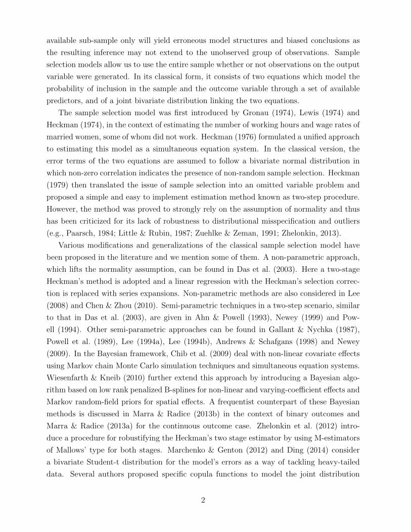
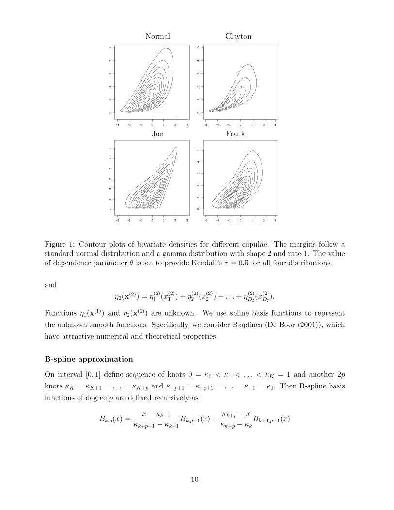
Archimedean copulae whereas Figure 1 shows the contour plots of bivariate densities for

normal and three Archimedean copulae (Clayton, Joe and Frank).

For Archimedean copulae we have

f2|1(y2|Y1 = 1) =1

P(Y1 = 1)f2(y2)

(1− ϕ′(F2)

ϕ′(Cθ)

),

where F2 = F2(y2) and Cθ = Cθ(F1(0), F2(y2)). Thus

E(Y ∗2 |Y1 = 1) =1

P(Y1 = 1)

(E (Y ∗2 )−

∫ ∞−∞

yf2(y)ϕ′(F2)

ϕ′(Cθ)dy

).

Hence the selection bias is equal to

1

P(Y1 = 1)

(P(Y1 = 0)E (Y ∗2 )−

∫ ∞−∞

yf2(y)ϕ′(F2)

ϕ′(Cθ)dy

).

Name Cθ(u, v) Parameter space Generator ϕ(t)

Clayton(u−θ + v−θ − 1

)−1/θθ ∈ (0,∞)

(t−θ − 1

)θ−1

Joe 1−[(1− u)θ + (1− v)θ − (1− u)θ(1− v)θ

]1/θθ ∈ (1,∞) − log

(1− (1− t)θ

)Frank −θ−1 log

[1 + (e−θu − 1)(e−θv − 1)/(e−θ − 1)

]θ ∈ R\ {0} − log e−θt−1

e−θ−1

Gumbel exp{−[(− log u)θ + (− log v)θ

]1/θ}θ ∈ [1,∞) (− log t)θ

AMH uv/ [1− θ(1− u)(1− v)] θ ∈ [−1, 1] log 1−θ(1−t)t

Table 1: Families of bivariate Archimedean copulae, with corresponding parameter range ofthe association parameter θ and generator ϕ(t).

3.2 Systematic component

Terms η1 and η2 are assumed to depend on sets of predictors x(1) and x(2), respectively, so

that η1 = η1(x(1)) and η2 = η2(x(2)), where x(1) = (x(1)1 , . . . , x

(1)D1

) and x(2) = (x(2)1 , . . . , x

(2)D2

).

Moreover, we assume the following additive form of the functions η1(x(1)) and η2(x(2))

η1(x(1)) = η(1)1 (x

(1)1 ) + η

(1)2 (x

(1)2 ) + . . .+ η

(1)D1

(x(1)D1

),

9

Normal Clayton

0.02 0.04 0.06

0.08

0.1

0.12

0.14

0.16

0.18

0.2

−3 −2 −1 0 1 2 3

01

23

45

0.05 0.1

0.15

0.2

0.25

−3 −2 −1 0 1 2 3

01

23

45

Joe Frank

0.02 0.04 0.06 0.08

0.1

0.12

0.14

0.16

0.18

0.2

−3 −2 −1 0 1 2 3

01

23

45

6

0.02 0.04

0.06

0.08

0.1

0.12

0.14

0.16

0.18

0.2

0.22

−3 −2 −1 0 1 2 3

01

23

45

Figure 1: Contour plots of bivariate densities for different copulae. The margins follow astandard normal distribution and a gamma distribution with shape 2 and rate 1. The valueof dependence parameter θ is set to provide Kendall’s τ = 0.5 for all four distributions.

and

η2(x(2)) = η(2)1 (x

(2)1 ) + η

(2)2 (x

(2)2 ) + . . .+ η

(2)D2

(x(2)D2

).

Functions η1(x(1)) and η2(x(2)) are unknown. We use spline basis functions to represent

the unknown smooth functions. Specifically, we consider B-splines (De Boor (2001)), which

have attractive numerical and theoretical properties.

B-spline approximation

On interval [0, 1] define sequence of knots 0 = κ0 < κ1 < . . . < κK = 1 and another 2p

knots κK = κK+1 = . . . = κK+p and κ−p+1 = κ−p+2 = . . . = κ−1 = κ0. Then B-spline basis

functions of degree p are defined recursively as

Bk,p(x) =x− κk−1

κk+p−1 − κk−1

Bk,p−1(x) +κk+p − xκk+p − κk

Bk+1,p−1(x)

10

for k = −p+ 1, . . . , K, with

Bk,0(x) =

{1, κk−1 ≤ x < κk

0 otherwise.

This gives K + p basis functions B−p+1,p(x), . . . , BK,p(x).

We approximate η(1)j (x) by a linear combination of basis functions:

K∑k=−p+1

αK,jBk,p(x) for j = 1, . . . , D1,

and, similarly, η(2)j (x) by

K∑k=−p+1

βK,jBk,p(x) for j = 1, . . . , D2.

In the remaining of the paper we omit the subscript p of basis functions Bk,p and we use

symbols B−p+1(x), . . . , BK(x) to denote p-th B-spline basis functions. We define vectors

αj ∈ Rp+K and βj ∈ Rp+K as

αj = (α−p+1,j, . . . , αK,j)T for j = 1, . . . , D1

and

βj = (β−p+1,j, . . . , βK,j)T for j = 1, . . . , D2

and vectors

α = (αT1 , . . . ,α

TD1

)T ∈ RD1(p+K)

and

β = (βT1 , . . . ,βTD1

)T ∈ RD2(p+K).

Moreover, we use the following notation throughout. For a given n ∈ N, assume that

(Y1i, Y2i)ni=1 are independent random variables related to predictors’ values x

(1)i = (x

(1)1i , . . . ,

x(1)D1i

) and x(2)i = (x

(2)1i , . . . , x

(2)D2i

) for i = 1, . . . , n such that Y1i = 1(Y ∗1i > 0) and Y2i = Y ∗2iY1i,

where Y ∗1i has density (7) with η1 = η1(x(1)i ) and Y ∗2i is distributed according to (6) with

η2 = η2(x(2)i ).

Let F1i, F2i denote the distribution functions of Y ∗1i and Y ∗2i and let Fi(·, ·) be the joint

cdf of the pair (Y ∗1i, Y∗

2i). Moreover, for j = 1, . . . , D1 let X(1)j : n × (p + K) be a matrix

11

defined through

X(1)j =

[B−p+k(x

(1)ji )]k=1,...,K, i=1,...,n

and for j = 1, . . . , D2 let X(2)j : n× (p+K) be a matrix defined as

X(2)j =

[B−p+k(x

(2)ji )]k=1,...,K, i=1,...,n

.

Then let X(1) : n×D1(p+K) and X(2) : n×D2(p+K) equal

X(1) =[X

(1)1 , . . . , X

(1)D1

]and

X(2) =[X

(2)1 , . . . , X

(2)D2

].

With the B-spline approximation, we postulate the parametric model

Y ∗1i ∼ N(X(1)i α, 1)

Y ∗2i ∼ f2i(y2|X(2)i ) = exp

(y2X

(2)i β − b(X(2)

i β) + c(y2)) (10)

where X(1)i and X

(2)i denote the i-th rows of the matrices X(1) and X(2), respectively.

4 Some estimation details

In order to estimate parameters α, β and θ, we employ a penalized likelihood approach

which is common for regression spline models. Based on (9) and (10), the log-likelihood

given a random sample (Y1i, Y2i)ni=1 equals

`(α,β, θ) =n∑i=1

(1−Y1i) logF1i(0)+Y1i(X(2)i βY2i−b(X(2)

i β)+c(Y2i)+log (1− z(Y2i,α,β, θ)) ,

(11)

where z(Y2i,α,β, θ) = ∂∂vCθ(F1i(0), v)

∣∣v→F2i(Y2i)

. The normality of Y ∗1i implies that F1i(0) =

Φ(−η1i), where Φ denotes the standard normal distribution function. The penalized log-

likelihood equals

`p(α,β, θ) = `(α,β, θ)− 1

2

D1∑j=1

λ(1)j αTj ∆T

m∆mαj −1

2

D2∑j=1

λ(2)j βTj ∆T

m∆mβj =

= `(α,β, θ)− 1

2αTQ(1)

m (λ(1))α− 1

2βTQ(2)

m (λ(2))β, (12)

12

where ∆m : (K + p−m)× (K + p) is the m-th difference matrix (Marx and Eilers, 1998),

Q(1)m (λ(1)) = diag(λ

(1)1 ∆T

m∆m, . . . , λ(1)D1

∆Tm∆m), Q

(2)m (λ(2)) = diag(λ

(2)1 ∆T

m∆m, . . . , λ(2)D2

∆Tm∆m),

and λ(1) = (λ(1)1 , . . . , λ

(1)D1

) and λ(2) = (λ(2)1 , . . . , λ

(2)D2

) are smoothing parameters controlling

the trade-off between smoothness and fitness.

For a given λ = (λ(1), λ(2)), we seek to maximize (12). In practice, an iterative procedure

based on a trust region approach can be used to achieve this. This method is generally more

stable and faster than its line-search counterparts (such as Newton-Raphson), particularly

for functions that are, for example, non-concave and/or exhibit regions that are close to flat;

see Nocedal & Wright (2006, Chapter 4) for full details. Such functions can occur relatively

frequently in bivariate models, often leading to convergence failures (Andrews, 1999; Butler,

1996; Chiburis et al., 2012). Some details related to the process of iterative maximization

of the penalized likelihood via a trust region algorithm are presented in subsection A.1 of

Appendix A.

Data-driven and automatic smoothing parameter estimation is pivotal for practical mod-

eling, especially when the data are partly censored as in our case, and each model equation

contains more than one smooth component. An automatic approach allows us to determine

the shape of the smooth functions from the data, hence avoiding arbitrary decisions by

the researcher as to the relevant functional form for continuous variables. For single equa-

tion spline models, there are a number of methods for automatically estimating smoothing

parameters within a penalized likelihood framework; see Ruppert et al. (2003) and Wood

(2006) for excellent detailed overviews. In our context, we propose to use the smoothing

approach based on Un-Biased Risk Estimator as detailed in subsection A.2 of Appendix A.

5 Asymptotic theory

In this section, the asymptotic consistency of the linear predictor η2 based on the penalized

maximum likelihood estimators for the regression equation of interest is shown. In particular,

the asymptotic rate of the mean squared error of η2 is derived. The theoretical considera-

tions also allows to derive its asymptotic bias and variance and its approximate distribution.

First, we introduce the notation that we use throughout. Denote δ = (α,β, θ) and let

Gn(δ) =(Gαn (δ), Gβ

n(δ), Gθn(δ)

),

where

Gαn (δ) =

∂`

∂α(δ) =

(∂`

∂α1

, . . . ,∂`

∂αD1

)∈ RD1(K+p+1),

13

Gβn(δ) =

∂`

∂β(δ) =

(∂`

∂β1

, . . . ,∂`

∂βD2

)∈ RD1(K+p+1),

and

Gθn(δ) =

∂`

∂θ(δ) ∈ R.

Analogically, let

Gn,p(δ) =(Gαn,p(δ), Gβ

n,p(δ), Gθn,p(δ)

)=

(∂`p∂α

(δ),∂`p∂β

(δ),∂`p∂θ

(δ)

).

Proceeding to the hessian matrix, let us denote

Hαn (δ) =

∂2`

∂α∂αT(δ), Hβ

n (δ) =∂2`

∂β∂βT(δ), Hβ,α

n (δ) =∂2`

∂α∂βT(δ) and so on.

Moreover, let

Hn(δ) =

Hαn (δ) Hα,β

n (δ) Hα,θn (δ)

Hβ,αn (δ) Hβ

n (δ) Hβ,θn (δ)

Hθ,αn (δ) Hθ,β

n (δ) Hθ,θn (δ)

.Analogically, let

Hαn,p(δ) =

∂2`p∂α∂αT

(δ) = Hαn (δ)−Q(1)

m (λ(1)n ),

Hβn,p(δ) =

∂2`p∂β∂βT

(δ) = Hβn (δ)−Q(2)

m (λ(2)n ),

and so on, and Hn,p(δ) = ∂2`p∂δ∂δT

(δ).

Let

Fαn (δ) = E [Hα

n (δ)] , Fβn (δ) = E

[Hβn (δ)

], Fα,β

n (δ) = E[Hα,βn (δ),

]Fαn,p(δ) = Fα

n (δ)−Q(1)m (λ(1)

n ), Fβn,p(δ) = Fβ

n (δ)−Q(2)m (λ(2)

n ).

Let δ0 denote a parameter vector that satisfies the condition EGn(δ0) = 0. Then δ0 is

maximizer of the expected unpenalized log-likelihood and provides the best approximation

of (η1, η2) in terms of Kullback-Leibler measure as it minimizes Kullback-Leibler distance.

We adopt the following assumptions:

A1. All partial derivatives up to the order 3 of copula function Cθ(u, v) w.r.t u, v and θ

exist and are bounded.

A2. The function z(y2,α,β, θ) is bounded away from 1.

A3. maxl=1,2; j=1,...,Dl

(λ

(l)j

)= O (nγ) where γ ≤ 2

2p+3.

14

A4. The explanatory variables x(1) and x(1) are distributed on unit cubes [0, 1]D1 and

[0, 1]D2 , respectively.

A5. The knots of the B-spline basis are equidistantly located so that κk − κk−1 = K−1n for

k = 1, . . . , Kn and the dimension of the spline basis satisfies Kn = O(n1/(2p+3)).

A6. Kn is such that (D1 +D2)(Kn + p) < n.

Theorem. Under assumptions (A1)-(A6) the estimate η(x) has asymptotic expansion

η(x)− η0(x) ≈ X(x)F−1p (δ0)Gp(δ

0),

which implies

MSE(η(x)) = E(η(x)− η0(x))2 = O(n−(2p+2)/(2p+3)).

Before we proceed to the proof of the theorem we derive analytic formulae for the gradient

and hessian of the penalized log-likelihood as their properties will play a central role in the

asymptotic considerations.

Gradient of the penalized likelihood

Straightforward calculations yield

Gαn,p(δ) = −

n∑i=1

{(1− Y1i)

(Φ(−X(1)

i α))−1

− Y1i∇Ci

1− zi

}ϕ(−X(1)

i α)X(1)i −αTQ(1)

m (λ(1)n ),

where ϕ(·) is the density function of the standard normal distribution and

∇Ci = ∂2

∂u∂vCθ(u, v)|u=F1i(0),v=F2i(Y2i) and zi = z(Y2i,α,β, θ). Moreover,

Gβn,p(δ) =

n∑i=1

Y1i

[Y2i − b′(X(2)

i β)− z′i1− zi

]X

(2)i − βTQ(2)

m (λ(2)n ),

where

z′i =∂zi∂η2

=∂2

∂v2Cθ(F1i(0), v)|v=F2i(Y2i)

∂F2i

∂η2

,

and

Gθn,p(δ) = −

n∑i=1

Y1i1

1− zi∂zi∂θ

,

where ∂zi∂θ

= ∂2

∂θ∂vCθ(F1i(0), v)|v=F2i(Y2i). Thus we can write the gradients in a matrix form

Gαn,p(δ) = aTX(1) −αTQ(1)

m (λ(1)n ),

15

where a = (a1, . . . , an) with ai = −{

(1− Y1i)(

Φ(−X(1)i α)

)−1

− Y1i∇Ci

1−zi

}ϕ(−X(1)

i α) for

i = 1, . . . , n. Analogically,

Gβn,p(δ) = bTX(2) − βTQ(2)

m (λ(2)n ),

where b = (b1, . . . , bn) with bi = Y1i

[Y2i − b′(X(2)

i β)− z′i1−zi

]for i = 1, . . . , n. Moreover,

Gθn,p(δ) = cT1,

where c = (c1, . . . , cn) with ci = −Y1i1

1−zi∂zi∂θ

and 1 = (1, . . . , 1)T ∈ Rn.

Hessian

Straightforward but tedious calculations yield the following lemma.

Lemma 1. The component matrices of Hn(δ) take the following forms:

Hαn (δ) =

(X(1)

)TW1X

(1), Hβn (δ) =

(X(2)

)TW2X

(2), Hα,βn (δ) =

(X(1)

)TW3X

(2),

Hθ,αn (δ) = 1TW4X

(1), Hθ,βn (δ) = 1TW5X

(2), Hθ,θn (δ) = 1TW61,

where Wj = diag(w(j)1 , . . . , w

(j)n ) for j = 1, . . . , 6 and

w(1)i = (1− Y1i)(F1i(0))−1(F1i(0)−1ϕ(−X(1)

i α)− 1)ϕ(−X(1)i α)+ (13)

+Y1i

{[1

1− zi∂3Ci∂u2∂v

−(∇Ci

1− zi

)2]ϕ(−X(1)

i α)− ∇Ci1− zi

}ϕ(−X(1)

i α),

w(2)i = Y1i

[−b′′(X(2)

i β) +1

(1− zi)2

(z′′i (1− zi) + (z′i)

2)], (14)

w(3)i = Y1i

[1

1− zi∂3Ci∂u2∂v

+z′i

(1− zi)2∇Ci

]where z′′i =

∂z′i∂η2

, (15)

w(4)i =

∂

∂θ

∇Ci1− zi

φ(−X(1)i α), (16)

w(5)i = −Y1i

∂

∂θ

z′i1− zi

, (17)

w(6)i = −Y1i

∂

∂θ

(1

1− zi∂zi∂θ

). (18)

16

Corollary 1. The Hessian Hn(δ) can be written in the following matrix form

Hn(δ) =

(X(1)

)T0 0

0(X(2)

)T0

0 0 1T

W1 W3 W4

W3 W2 W5

W4 W5 W6

X(1) 0 0

0 X(2) 0

0 0 1

where the matrices Wj = diag(w

(j)1 , . . . , w

(j)n ) for j = 1, . . . , 6 are given by the expressions

(13)-(18).

In order to proof Theorem, we use several lemmas, stated below.

Lemma 2. Under assumptions (A1)-(A6), elements of the matrix Fn(δ0) are of order

O(

nKn

)and elements of the matrix Fn,p(δ

0) are of order O(

nKn

+ maxl=1,2; j=1,...,Dlλ

(l)j K

2pn

).

Lemma 3. Under assumptions (A1)-(A6), elements of the matrix (Fn,p(δ0))−1

are of order

OP

(Kn

n

).

Lemma 4. Elements of the matrix Hn(δ0)− Fn(δ0) are of order OP

(nk

).

The proofs of Lemmas 2 - 4 are presented in Appendix B.

Proof of Theorem. First, we expand Gp(·) around δ0. Let Mn = (D1 +D2)(Kn + p). For

j = 1, . . . , D1 +D2 + 1

0 =∂lp∂δj

(δ) =∂lp∂δj

(δ0) +Mn∑l=1

∂2lp∂δj∂δl

(δ0)(δl − δ0,l)+

+Mn∑l=1

Mn∑r=1

(δl − δ0,l)∂3lp

∂δj∂δl∂δr(δ0)(δr − δ0,r) + o(Rn),

where Rn =∑Mn

l=1

∑(D1+D2)(Kn+p)r=1 (δl − δ0,l) ∂3lp

∂δj∂δl∂δr(δ0)(δr − δ0,r).

17

Series inversion yields

δj − δj0 = −Mn∑l=1

ajl∂lp∂δl

(δ0) +1

2

Mn∑l=1

Mn∑r=1

bjlr∂lp∂δl

(δ0)∂lp∂δr

(δ0) + . . .

where ajl is (j, l)-element of the inverse of matrix Hp(δ0) and

bjlr =∑Mn

s=1

∑Mn

t=1

∑Mn

u=1 ajsaltaru∂3lp

∂δs∂δt∂δu(δ0).

Then (Hp(δ

0))−1

=(Fp(δ

0) +(Hp(δ

0)− Fp(δ0)))−1

=(Fp(δ

0) + S(δ0))−1

=

= Fp(δ0)−1 − Fp(δ0)−1S(δ0)Fp(δ

0)−1 + Fp(δ0)−1S(δ0)Fp(δ

0)−1S(δ0)Fp(δ0)−1 + . . . =

= Fp(δ0)−1

(I − S(δ0)Fp(δ

0)−1 + S(δ0)Fp(δ0)−1S(δ0)Fp(δ

0)−1 + . . .)

=

= Fp(δ0)−1

(I +O

(√Kn/n

)).

Moreover,∂3lp

∂δs∂δt∂δu(δ0) =

n∑i=1

∂wi∂δs

B−p+t(xi)B−p+u(xi) = OP (n/Kn),

as∑n

i=1B−p+t(xi)B−p+u(xi) = O(n/Kn) and ∂wi

∂δsis bounded. This yields bjlr = O(K2

n/n2)

and in consequenceMn∑l=1

Mn∑r=1

bjlr∂lp∂δl

(δ0)∂lp∂δr

(δ0) = op(Kn/n).

Thus

δj − δ0,j =Mn∑l=1

ajl

(−∂lp∂δl

(δ0)

)+ oP (Kn/n) =

=Mn∑l=1

fjl

(−∂lp∂δl

(δ0)

)(1 + o(1)) + oP (Kn/n),

where fjl is (j, l)-element of the matrix Fp(δ0)−1. Hence we can write the above equation in

a matrix form

δ − δ0 = −Fp(δ0)−1Gp(δ0)(1 + o(1)) + oP (Kn/n). (19)

Thus assumptions (A3) and (A5) together with the fact that E(G(δ0)) = 0 yield

E∣∣∣∣η(x)− η0(x)

∣∣∣∣2 = E(X(x)δ −X(x)δ0)(X(x)δ −X(x)δ0)T = O(K−(p+1)n + λjnK

1−mn /n).

Hence E||η(x)− η0(x)||2 = O(n−(2p+2)/(2p+3)).�

18

Remark Expansion (19) yields the approximate variance of η(x) in the form

Var(η(x)) ≈ X(x)Fp(δ0)−1F (δ0)Fp(δ

0)−1X(x)T ,

which can be shown to be of order O(Kn/n) as n→∞. Moreover, using the Central Limit

Theorem we obtain the approximate distribution of η(x) as

η(x)a∼ N(η0(x),Var(η(x))).

6 Simulations

In this section, the properties of the proposed generalized additive sample selection model

are investigated empirically. Specifically, we first assess the effectiveness of the proposed

approach at finite sample sizes and then provide some evidence of the potential inaccuracy

arising from modeling transformed outcomes.

6.1 Empirical consistency

Data were generated as follows. For the latent selection variable, it was assumed that

Y ∗1i = α0 + s1(x1) + s2(x2) + α4x4 + α5x5 + εi,

with α0 = 0.7, s1(x) = −0.2 sin( π46x), s2(x) = −0.0004(x + 0.01x1/3), α4 = 0.6, α5 = −0.4

and εi ∼ N(0, 1), whereas the outcome variable Y ∗2i was assumed to pertain to a gamma

distribution with shape parameter k = 2 and expected value µi = E(Y ∗2i) such that

log(µi) = β0 + s3(x1) + s4(x3) + β4x4 + β5x5,

with β0 = −1.5, s3(x) = 0.0006 exp(0.1x), s4(x) = 0.03x, β4 = −1 and β5 = 0.75. The two

equations were linked using a Gumbel copula with association parameter θ = 3. The co-

variates were generated as x1 ∼ Uniform(16, 66), x2 ∼ Uniform(10, 70), x3 ∼ Uniform(0, 20)

and x4 and x5 were binary variables taking values 0 and 1 with equal probabilities.

To investigate the asymptotic behavior of the estimators, data sets of increasing sizes

were considered: n = 500, 1000, 1500, 2000, 2500, 3000. For each generated data set a gen-

eralized additive sample selection model assuming a gamma distribution for the outcome

with log link function was fitted using the SemiParSampleSel function from the package

SemiParSampleSel (Wojtys et al., 2015) in R (R Core Team, 2015). Additionally, a univari-

ate generalized additive model based only on the observed outcomes was fitted for compari-

19

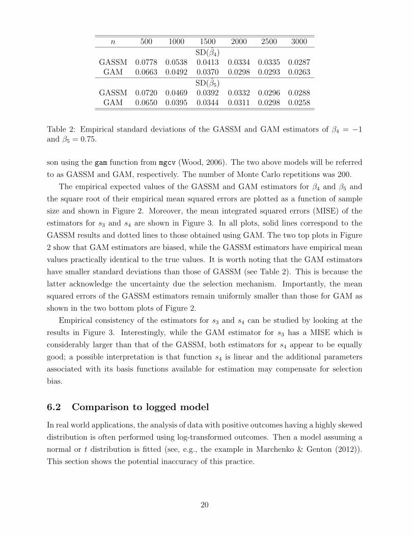
n 500 1000 1500 2000 2500 3000

SD(β4)GASSM 0.0778 0.0538 0.0413 0.0334 0.0335 0.0287

GAM 0.0663 0.0492 0.0370 0.0298 0.0293 0.0263

SD(β5)GASSM 0.0720 0.0469 0.0392 0.0332 0.0296 0.0288

GAM 0.0650 0.0395 0.0344 0.0311 0.0298 0.0258

Table 2: Empirical standard deviations of the GASSM and GAM estimators of β4 = −1and β5 = 0.75.

son using the gam function from mgcv (Wood, 2006). The two above models will be referred

to as GASSM and GAM, respectively. The number of Monte Carlo repetitions was 200.

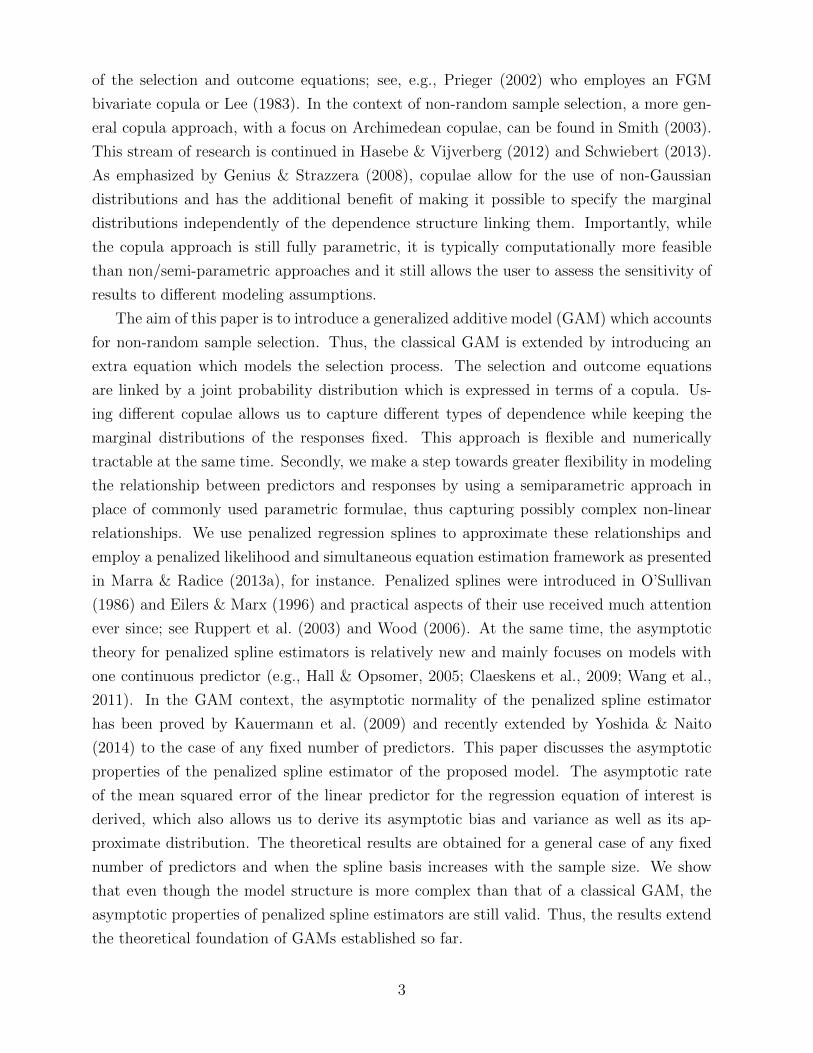
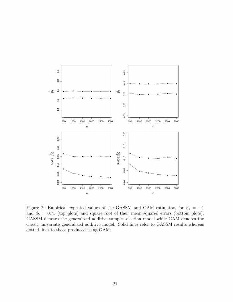
The empirical expected values of the GASSM and GAM estimators for β4 and β5 and

the square root of their empirical mean squared errors are plotted as a function of sample

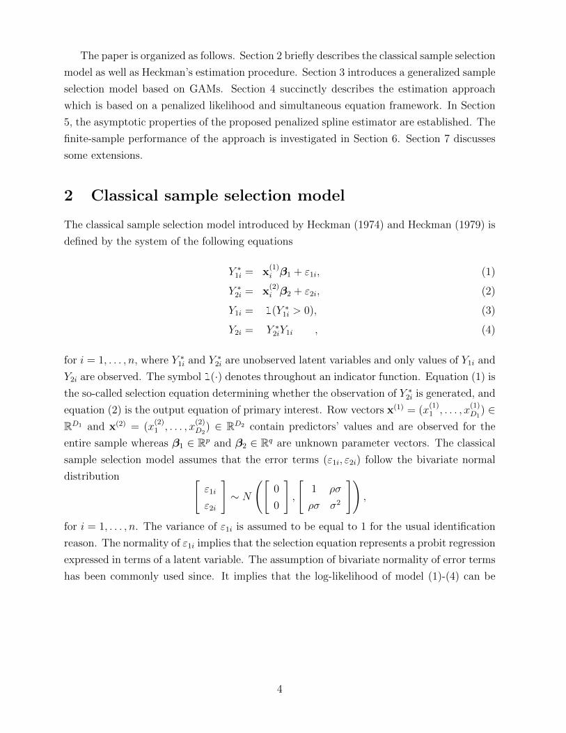
size and shown in Figure 2. Moreover, the mean integrated squared errors (MISE) of the

estimators for s3 and s4 are shown in Figure 3. In all plots, solid lines correspond to the

GASSM results and dotted lines to those obtained using GAM. The two top plots in Figure

2 show that GAM estimators are biased, while the GASSM estimators have empirical mean

values practically identical to the true values. It is worth noting that the GAM estimators

have smaller standard deviations than those of GASSM (see Table 2). This is because the

latter acknowledge the uncertainty due the selection mechanism. Importantly, the mean

squared errors of the GASSM estimators remain uniformly smaller than those for GAM as

shown in the two bottom plots of Figure 2.

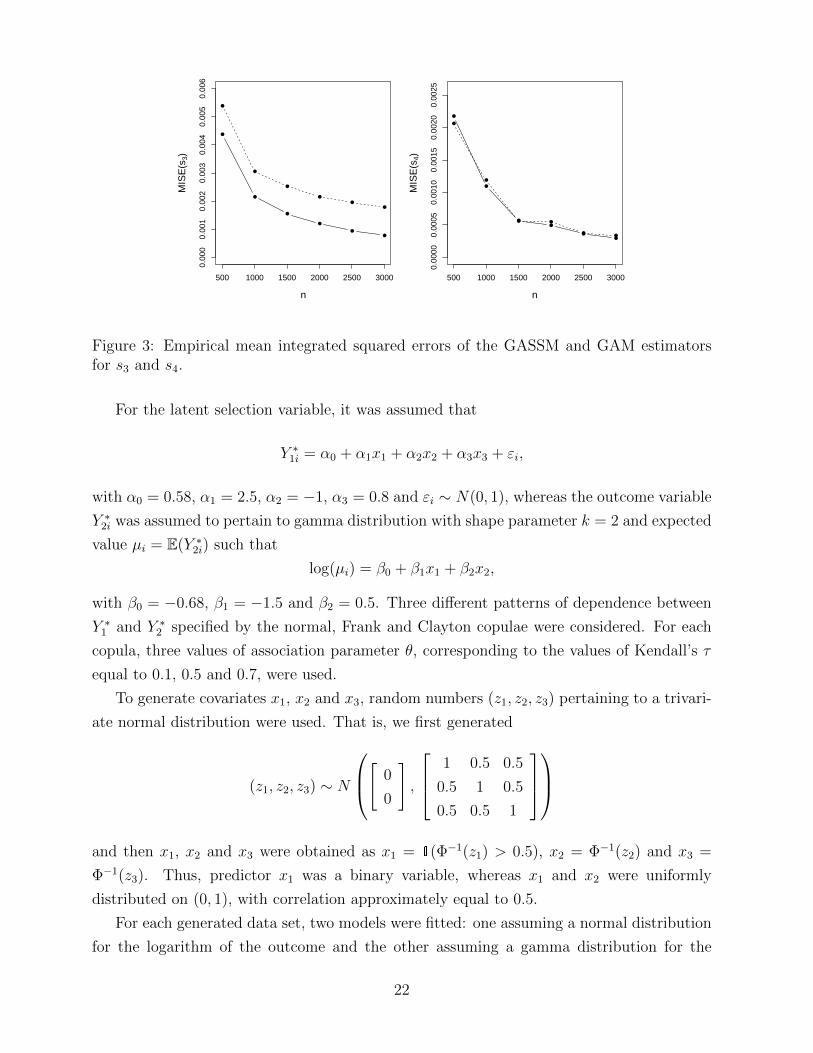
Empirical consistency of the estimators for s3 and s4 can be studied by looking at the

results in Figure 3. Interestingly, while the GAM estimator for s3 has a MISE which is

considerably larger than that of the GASSM, both estimators for s4 appear to be equally

good; a possible interpretation is that function s4 is linear and the additional parameters

associated with its basis functions available for estimation may compensate for selection

bias.

6.2 Comparison to logged model

In real world applications, the analysis of data with positive outcomes having a highly skewed

distribution is often performed using log-transformed outcomes. Then a model assuming a

normal or t distribution is fitted (see, e.g., the example in Marchenko & Genton (2012)).

This section shows the potential inaccuracy of this practice.

20

● ● ● ● ● ●

500 1000 1500 2000 2500 3000

−1.

4−

1.2

−1.

0−

0.8

−0.

6

n

β 4^ ● ● ● ● ● ●

●● ● ●

● ●

500 1000 1500 2000 2500 3000

n

β 5^

●● ● ●

●●

0.55

0.65

0.75

0.85

0.95

●

● ● ● ● ●

500 1000 1500 2000 2500 3000

0.00

0.05

0.10

0.15

0.20

0.25

n

RM

SE

(β4^)

●

●

●● ●

●

●

● ● ●●

●

500 1000 1500 2000 2500 3000

0.00

0.05

0.10

0.15

0.20

n

RM

SE

(β5^)

●

●

●●

● ●

Figure 2: Empirical expected values of the GASSM and GAM estimators for β4 = −1and β5 = 0.75 (top plots) and square root of their mean squared errors (bottom plots).GASSM denotes the generalized additive sample selection model while GAM denotes theclassic univariate generalized additive model. Solid lines refer to GASSM results whereasdotted lines to those produced using GAM.

21

●

●

●

●●

●

500 1000 1500 2000 2500 3000

0.00

00.

001

0.00

20.

003

0.00

40.

005

0.00

6

n

MIS

E(s

3)

●

●

●

●

●●

●

●

● ●

●●

500 1000 1500 2000 2500 3000

0.00

000.

0005

0.00

100.

0015

0.00

200.

0025

n

MIS

E(s

4)

●

●

●●

●●

Figure 3: Empirical mean integrated squared errors of the GASSM and GAM estimatorsfor s3 and s4.

For the latent selection variable, it was assumed that

Y ∗1i = α0 + α1x1 + α2x2 + α3x3 + εi,

with α0 = 0.58, α1 = 2.5, α2 = −1, α3 = 0.8 and εi ∼ N(0, 1), whereas the outcome variable

Y ∗2i was assumed to pertain to gamma distribution with shape parameter k = 2 and expected

value µi = E(Y ∗2i) such that

log(µi) = β0 + β1x1 + β2x2,

with β0 = −0.68, β1 = −1.5 and β2 = 0.5. Three different patterns of dependence between

Y ∗1 and Y ∗2 specified by the normal, Frank and Clayton copulae were considered. For each

copula, three values of association parameter θ, corresponding to the values of Kendall’s τ

equal to 0.1, 0.5 and 0.7, were used.

To generate covariates x1, x2 and x3, random numbers (z1, z2, z3) pertaining to a trivari-

ate normal distribution were used. That is, we first generated

(z1, z2, z3) ∼ N

[ 0

0

],

1 0.5 0.5

0.5 1 0.5

0.5 0.5 1

and then x1, x2 and x3 were obtained as x1 = 1(Φ−1(z1) > 0.5), x2 = Φ−1(z2) and x3 =

Φ−1(z3). Thus, predictor x1 was a binary variable, whereas x1 and x2 were uniformly

distributed on (0, 1), with correlation approximately equal to 0.5.

For each generated data set, two models were fitted: one assuming a normal distribution

for the logarithm of the outcome and the other assuming a gamma distribution for the

22

β0 β1 β2 τ Test

Bias (%) RMSE Bias (%) RMSE Bias (%) RMSE Bias (%) RMSE error

Normal Copula

τ=

0.1 G -5.7 0.129 3.8 0.15 5.3 0.105 -83.5 0.249 0.329

L 23.7 0.253 9.7 0.272 11.9 0.141 -227.4 0.426 0.339

τ=

0.5 G -0.4 0.069 0.7 0.077 1.9 0.086 -1 0.13 0.321

L 30.9 0.236 5.3 0.153 5.9 0.111 -19.3 0.243 0.334

τ=

0.7 G -0.1 0.06 0.5 0.066 1.9 0.084 0.3 0.104 0.321

L 32.3 0.229 4.2 0.096 4.1 0.098 -7.1 0.121 0.332

Frank Copula

τ=

0.1 G -6.1 0.13 3.2 0.148 0.5 0.094 -34 0.245 0.328

L 39.7 0.32 -0.4 0.204 -3.5 0.12 18.9 0.318 0.347

τ=

0.5 G -2.7 0.085 1.4 0.095 -0.3 0.084 -6.8 0.18 0.324

L 33 0.249 3.2 0.132 -0.6 0.102 -5.1 0.205 0.338

τ=

0.7 G -1.6 0.07 0.8 0.078 -0.3 0.084 -2.5 0.149 0.324

L 30.8 0.225 4.2 0.112 0.1 0.098 -5.9 0.156 0.335

Clayton Copula

τ=

0.1 G 1.3 0.058 -0.4 0.064 1.9 0.094 5.5 0.071 0.322

L 32.3 0.227 3.9 0.086 4.9 0.107 -76.5 0.085 0.332

τ=

0.5 G 0.6 0.047 0 0.054 1.4 0.086 1.7 0.06 0.321

L 32.4 0.229 4.1 0.091 4.7 0.101 -7.9 0.093 0.332

τ=

0.7 G 0.4 0.045 0.1 0.05 1.1 0.085 1.4 0.052 0.32

L 33.5 0.233 3.6 0.077 4.1 0.097 -1.8 0.053 0.332

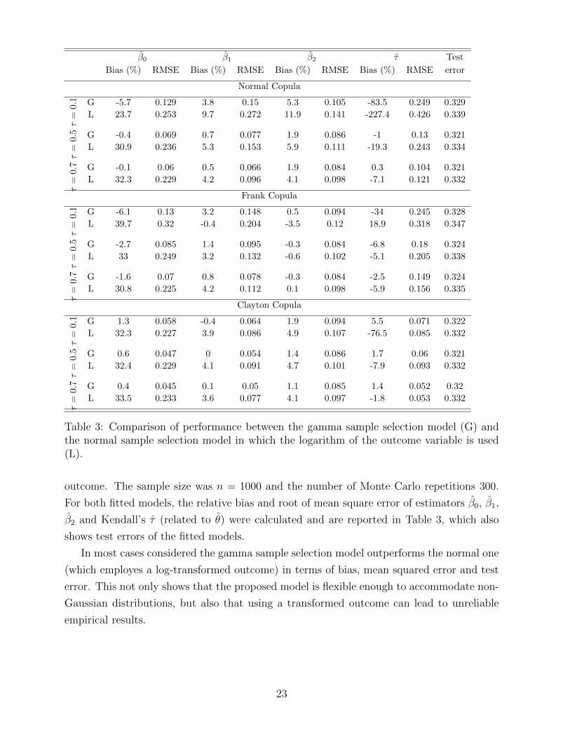
Table 3: Comparison of performance between the gamma sample selection model (G) andthe normal sample selection model in which the logarithm of the outcome variable is used(L).

outcome. The sample size was n = 1000 and the number of Monte Carlo repetitions 300.

For both fitted models, the relative bias and root of mean square error of estimators β0, β1,

β2 and Kendall’s τ (related to θ) were calculated and are reported in Table 3, which also

shows test errors of the fitted models.

In most cases considered the gamma sample selection model outperforms the normal one

(which employes a log-transformed outcome) in terms of bias, mean squared error and test

error. This not only shows that the proposed model is flexible enough to accommodate non-

Gaussian distributions, but also that using a transformed outcome can lead to unreliable

empirical results.

23

7 Discussion

We have introduced an extension of the generalized additive model which accounts for non-

random sample selection. The proposed approach is flexible in that it allows for different dis-

tributions of the outcome variable, several dependence structures between the outcome and

selection equations, and non-parametric effects on the responses. Parameter estimation with

integrated automatic multiple smoothing parameter selection is achieved within a penalized

likelihood and simultaneous equation framework. We have established the asymptotic the-

ory for the proposed penalized spline estimators, and illustrated the empirical effectiveness

of the approach through a simulation study. A few points are noteworthy.

• The generalized sample selection model has been formulated using penalized B-splines.

This allows for simple handling of the model’s theoretical properties. However, in

practice different smoothers can be used, for example truncated polynomials (which

yield an equivalent approach as detailed in Kauermann et al. (2009)) or thin plate

regression splines (Wood, 2006) .

• The estimation procedure discussed in Section 4 has been implemented in the freely

available R package SemiParSampleSel. Currently, the outcome can be modeled using

the normal, gamma and a number of discrete distributions. The copulae available

are: normal, Clayton, Joe, Frank, Gumbel, AMH, FGM and their rotated versions.

Given the modular structure of the estimation algorithm, other copulae and marginal

distributions can be incorporated in SemiParSampleSel with little programming work.

• For simplicity of treatment and notation, the generalized additive sample selection

model has been defined using as few parameters as possible. However, many model

structures are allowed within the proposed framework. For example, the association

parameter θ can be made dependent on predictors and hence enter the likelihood func-

tion as a transformed linear predictor instead of a scalar. Similarly, even though the

scale parameter φ has been set to 1 for simplicity of derivations, additional parameters

related to the specific distribution employed can be estimated. In both cases, all the

theoretical derivations presented in the paper still hold.

• Assumption A4 in Section 5 allows the sequence smoothing parameters λn to grow

as the sample size increases. This condition is rather week as, in fact, the sequence

λn based on the mean squared error criterion described in Section A.2 is bounded in

probability (cf e.g., Kauermann, 2005). Thus the theoretical properties of the penalized

estimator derived in Section 5 hold even if the smoothing parameters are estimated,

and not deterministic.

24

An interesting direction of future research will be to compare the small sample per-

formances of the proposed estimator and some of the non-parametric, semiparametric and

Bayesian methods mentioned in the introduction. Moreover, for many copulae a specific

value of the association parameter θ yields a product distribution which indicates lack of

non-random sample selection. Thus, the important issue of testing hypotheses regarding

parameter θ will be addressed in future work.

Acknowledgements

This research was supported by the Engineering and Physical Sciences Research Council,

UK (Grant EPJ0067421).

A Algorithmic details

A.1 Trust region algorithm

Recall that δ = (α,β, θ) and define the penalized gradient and Hessian at iteration a as

G[a]p = G[a]−Sλδ

[a] and H[a]p = H [a]−Sλ. Each iteration of the trust region algorithm solves

the problem

minp

˘p(δ

[a])def= −

{`p(δ

[a]) + pTG[a]p +

1

2pTH [a]

p p

}such that ‖p‖ ≤ r[a],

δ[a+1] = arg minp

˘p(δ

[a]) + δ[a],

where ‖ · ‖ denotes the Euclidean norm, and r[a] is the radius of the trust region. At

each iteration of the algorithm, ˘p(δ

[a]) is minimized subject to the constraint that the

solution falls within a trust region with radius r[a]. The proposed solution is then accepted

or rejected and the trust region expanded or shrunken based on the ratio between the

improvement in the objective function when going from δ[a] to δ[a+1] and that predicted by

the quadratic approximation. See Geyer (2013) for the exact details (e.g., numerical stability

and termination criteria) of the implementation used here. It is important to stress that near

the solution the trust region method typically behaves as a classic unconstrained algorithm

(Geyer, 2013; Nocedal & Wright, 2006). Starting values for the coefficients in α and β are

obtained by fitting the selection and outcome equations separately. The initial parameter

of θ is set to zero as there is not typically good a priori information about the direction

and strength of the association between the selection and outcome equations, conditional

on covariates.

25

A.2 Multiple smoothing parameter estimation

Let us use the fact that near the solution the trust region algorithm usually behaves as a

classic Newton or Fisher Scoring method, and assume that δ[a+1] is a new updated guess

for the parameter vector which maximizes `p. If δ[a+1] is to be ‘correct’, then the penalized

gradient evaluated at those parameter values would be 0, i.e. G[a+1]p = 0. Applying a first

order Taylor expansion to G[a+1]p about δ[a] yields 0 = G

[a+1]p ≈ G

[a]p +

(δ[a+1] − δ[a]

)H

[a]p ,

from which we find the solution at iteration a + 1. After some manipulation, this can be

expressed as

δ[a+1] =(I [a] + Sλ

)−1√I [a]z[a],

where I [a] is −H [a] (or, alternatively, −E(H [a]

)), and z[a] =

√I [a]δ[a] + ε[a], with ε[a] =√

I [a]−1

G[a]. From standard likelihood theory, ε ∼ N (0, I) and z ∼ N (µz, I), where I is

an identity matrix, µz =√Iδ0, and δ0 is the true parameter vector. The predicted value

vector for z is µz =√I δ = Aλz, where Aλ =

√I (I + Sλ)−1

√I. Since our goal is to

select the smoothing parameters in as parsimonious manner as possible so that the smooth

terms’ complexity which is not supported by the data is suppressed, λ is estimated so that

µz is as close as possible to µz. This can be achieved using

E(‖µz − µz‖2

)= E

(‖z−Aλz− ε‖2

)= E

(‖z−Aλz‖2

)+ E

(−εTε− 2εTµz + 2εTAλµz + 2εTAλε

)= E

(‖z−Aλz‖2

)− n+ 2tr(Aλ),

where n = 3n and tr(Aλ) is the number of effective degrees of freedom of the penalized

model. Hence, the smoothing parameter vector is estimated by minimizing an estimate of

the expectation above, that is

V(λ) = ‖z−Aλz‖2 − n+ 2tr(Aλ), (20)

which is equivalent to the expression of the Un-Biased Risk Estimator given in Wood (2006,

Chapter 4). This is also equivalent to the Akaike information criterion after dropping the

irrelevant constant; the first term on the right hand side of (20) is a quadratic approximation

to −2`(δ) to within an additive constant. In practice, given δ[a+1], the problem becomes

λ[a+1] = arg minλ

V(λ)def= ‖z[a+1] −A

[a+1]λ z[a+1]‖2 − n+ 2tr(A

[a+1]λ ), (21)

which is solved using the automatic stable and efficient computational routine by Wood

(2004).

26

B Proofs of Lemmas

Proof of Lemma 2. We have

Fn(δ0) =

(X(1)

)T0 0

0(X(2)

)T0

0 0 1T

Eδ0(W1) Eδ0(W3) Eδ0(W4)

Eδ0(W3) Eδ0(W2) Eδ0(W5)

Eδ0(W4) Eδ0(W5) Eδ0(W6)

X(1) 0 0

0 X(2) 0

0 0 1

.

From Lemma 1 of Yoshida & Naito (2012) we obtain that elements of matrices(X

(1)j

)TX

(1)j

are of order O(

nKn

)for j = 1, . . . , D1, and elements of matrices

(X

(1)j

)TX

(1)l are of order

O(

nK2

n

)for j 6= l, j, l = 1, . . . , D1. The same boundaries hold for the matrices X

(2)j ,

j = 1, . . . , D2.

Thus elements of matrices(X(1)

)TX(1) and

(X(2)

)TX(2) are of order O

(nKn

). In a straight-

forward way, the result also extends to the matrix(X(1)

)TX(2).

Now we consider the order of the diagonal elements w(1)i , . . . , w

(6)i . It holds∣∣∣∣∂F2i

∂η2i

(y2)

∣∣∣∣ =

∣∣∣∣∫ y2

−∞(v − b′(β0))f2i(v)dv

∣∣∣∣ ≤ Eδ0|Y2i|+ |b′(β0)| ≤ 2Eδ0|Y2i|. (22)

and∂2F2i

∂η22i

(y2) =

∫ y2

−∞

(1− b′′(η2i) + (v − b′(η2i))

2)f2i(v)dv. (23)

Thus |∂2F2i

∂η22i(y2)| ≤ 1+2Varδ0(Y2i). This combined with (22) and assumptions (A1) and (A2)

yields E(w(j)i ) = O(1) for j = 1, . . . , 6.

Moreover, by the properties of B-spline basis the (i, l)th components of(X

(1)j

)TX

(1)k , for

j, k = 1, . . . , D1, and(X

(2)j

)TX

(2)k , for j, k = 1, . . . , D2, equal 0 if |i − l| > p. Hence the

matrices(X(1)

)TW1X

(1),(X(2)

)TW2X

(2) are band matrices and the assertion follows.�

Proof of Lemma 3. We use induction w.r.t. the number of variables. Let Mn = D1+D2+1

and matrix UMn be defined as

UMn = Fn,p(δ0) = α

[UMn−1 RT

R Λ

].

The result of Horn & Johnson (1985) yields

U−1Mn

=

[U−1Mn−1 + U−1

Mn−1RTV −1RU−1

Mn−1 −U−1Mn−1R

TV −1

−V −1RU−1Mn−1 U−1

Mn−1

],

27

where V −1 = Λ−RU−1Mn−1R

T . Then assertion can be proven similarly to Kauermann et al.

(2009) by using the fact that matrices(X(1)

)TW1X

(1),(X(2)

)TW1X

(2) and(X(1)

)TW1X

(2)

are band matrices and the properties of the inverse of band matrices listed in Demko (1977).�

Proof of Lemma 4 (sketch).

Hn(δ0)− Fn(δ0) = XT (W − E(W ))X.

It holds wi − E(wi) = OP (n−1/2) as every wi is a sum of independent and bounded random

variables. Moreover,1

n

n∑i=1

(B−p+j(xi)B−p+l(xi))2 = O(K−1

n ).

Hence∑n

i=1 Var(wiB−p+j(xi)B−p+l(xi)) = O(n/Kn) which yields the assertion.�

References

Ahn, H. & Powell, J. L. (1993). Semiparametric estimation of censored selection models

with a nonparametric selection mechanism. Journal of Econometrics, 58, 3–29.

Amemiya, T. (1985). Advanced Econometrics. Harvard University Press.

Andrews, D. W. (1999). Estimation when a parameter is on a boundary. Econometrica, 67,

1341–1383.

Andrews, D. W. K. & Schafgans, M. M. A. (1998). Semiparametric estimation of the

intercept of a sample selection model. Review of Economic Studies, 65, 497–517.

Butler, J. S. (1996). Estimating the correlation in censored probit models. The Review of

Economics and Statistics, 78, 356–358.

Chen, S. & Zhou, Y. (2010). Semiparametric and nonparametric estimation of sample

selection models under symmetry. Journal of Econometrics, 157, 143–150.

Chib, S., Greenberg, E., & Jeliazkov, I. (2009). Estimation of semiparametric models in the

presence of endogeneity and sample selection. Journal of Computational and Graphical

Statistic, 18, 321–348.

Chiburis, R. C., Das, J., & Lokshin, M. (2012). A practical comparison of the bivariate

probit and linear IV estimators. Economics Letters, 117, 762–766.

28

Claeskens, G., Krivobokova, T., & Opsomer, J. (2009). Asymptotic properties of penalized

spline estimators. Biometrika, 96, 529–544.

Collier, D. & Mahoney, J. (1996). Insights and pitfalls: selection bias in qualitative research.

World Politics, 49, 56–91.

Das, M., Newey, W., & Vella, F. (2003). Nonparametric estimation of sample selection

models. Review of Economic Studies, 70, 33–58.

De Boor, C. (2001). A practical guide to splines; revised edition. Applied mathematical

sciences. Berlin: Springer.

Demko, S. (1977). Inverses of band matrices and local convergence of spline projections.

SIAM Journal on Numerical Analysis, 14, 616–619.

Ding, P. (2014). Bayesian robust inference of sample selection using selection-models. Jour-

nal of Multivariate Analysis, 124, 451–464.

Eilers, P. & Marx, B. (1996). Flexible smoothing with B-splines and penalties. Statistical

Science, 11, 89–121.

Gallant, R. A. & Nychka, D. W. (1987). Semi-nonparametric maximum likelihood estima-

tion. Econometrica, 55, 363–390.

Genius, M. & Strazzera, E. (2008). Applying the copula approach to sample selection

modelling. Applied Economics, 40, 1443–1455.

Geyer, C. J. (2013). Trust regions. Available at http://cran.r-project.org/web/

packages/trust/vignettes/trust.pdf.

Gronau, R. (1974). Wage comparisons: A selectivity bias. Journal of Political Economy,

82, 1119–1143.

Guo, S. & Fraser, W. (2014). Propensity Score Analysis: Statistical Methods and Appli-

cations. Advanced Quantitative Techniques in the Social Sciences (Book 11). SAGE

Publications.

Hall, P. & Opsomer, J. (2005). Theory for penalized spline regression. Biometrika, 92,

105–118.

Hasebe, T. & Vijverberg, W. P. (2012). A Flexible Sample Selection Model: A GTL-Copula

Approach. IZA Discussion Papers 7003, Institute for the Study of Labor (IZA).

29

Hastie, T. J. & Tibshirani, R. J. (1990). Generalized additive models. London: Chapman &

Hall.

Heckman, J. (1974). Shadow prices, market wages, and labor supply. Econometrica, 42,

679–694.

Heckman, J. (1976). The common structure of statistical models of truncation, sample

selection and limited dependent variables and a simple estimator for such models. Annals

of Economic and Social Measurement, 5, 475–492.

Heckman, J. (1979). Sample selection bias as a specification error. Econometrica, 47, 153–

162.

Horn, R. A. & Johnson, C. A. (1985). Matrix Analysis. Cambridge University Press,

Cambridge.

Joe, H. (1997). Multivariate Models and Dependence Concepts. Chapman & Hall Ltd.,

London.

Kauermann, G., Krivobokova, T., & Fahrmeir, L. (2009). Some asymptotic results on

generalized penalized spline smoothing. J. R. Statist. Soc. B, 71, 487–503.

Lee, D. S. (2008). Training, wages, and sample selection: Estimating sharp bounds on

treatment effects. Review of Economic Studies, 76(11721), 1071–1102.

Lee, L. (1983). Generalized econometric models with selectivity. Econometrica, 51, 507–512.

Lee, L. F. (1994a). Semiparametric instrumental variable estimation of simultaneous equa-

tion sample selection models. Journal of Econometrics, 63, 341–388.

Lee, L. F. (1994b). Semiparametric two-stage estimation of sample selection models subject

to Tobit-type selection rules. Journal of Econometrics, 61, 305–344.

Lennox, C., Francis, J., & Wang, Z. (2012). Selection models in accounting research. The

Accounting Review, 87, 589–616.

Lewis, H. G. (1974). Comments on selectivity biases in wage comparisons. Journal of

Political Economy, 82, 1145–1155.

Little, R. J. & Rubin, D. B. (1987). Statistical Analysis with Missing Data. New York: John

Wiley & Sons.

Marchenko, J. V. & Genton, M. G. (2012). A Heckman selection-t model. Journal of the

American Statistical Association, 107, 304–317.

30

Marra, G. & Radice, R. (2013a). Estimation of a regression spline sample selection model.

Computational Statistics and Data Analysis, 61, 158–173.

Marra, G. & Radice, R. (2013b). A penalized likelihood estimation approach to semipara-

metric sample selection binary response modeling. Electronic Journal of Statistics, 7,

1432–1455.

Nelsen, R. (2006). An Introduction to Copulas. Springer-Verlag, New York, second edition.

Newey, W. K. (1999). Two-step series estimation of sample selection models. Technical

Report Working Paper no. 99-04, Cambridge, MA: Massachusetts Institute of Technology.

Newey, W. K. (2009). Two-step series estimation of sample selection models. Econometrics

Journal, 12, S217–S229.

Nocedal, J. & Wright, S. (2006). Numerical Optimization. Springer-Verlag, New York.

O’Sullivan, F. (1986). A statistical perspective on ill-posed inverse problems. Statistical

Science, 1, 505–527.

Paarsch, H. (1984). A monte carlo comparison of estimators for censored regression. Journal

of Econometrics, 24, 197–213.

Powell, J. L. (1994). Estimation of semiparametric models. In J. J. Heckman & E. Leamer

(Eds.), Handbook of econometrics (pp. 5307–5368). Amsterdam: Elsevier.

Powell, J. L., Stock, J. H., & Stoker, T. M. (1989). Semiparametric estimation of index

coefficients. Econometrica, 57, 1403–30.

Prieger, J. E. (2002). A flexible parametric selection model for non-normal data with appli-

cation to health care usage. Journal of Applied Econometrics, 17, 367–392.

Puhani, P. A. (2000). The Heckman correction for sample selection and its critique. Journal

of Economic Surveys, 14, 53–68.

R Core Team (2015). R: A Language and Environment for Statistical Computing. R Foun-

dation for Statistical Computing, Vienna, Austria.

Ruppert, D., Wand, M., & Carroll, R. (2003). Semiparametric Regression. Cambridge

University Press, New York.

Schweizer, B. (1991). Thirty years of copulas. In G. Dall’Aglio, S. Kotz, & G. Salinetti

(Eds.), Advances in Probability Distributions with Given Marginals: Beyond the Copulas

chapter 2, (pp. 13–50). Dordrecht: Kluwer.

31

Schwiebert, J. (2013). Sieve Maximum Likelihood Estimation of a Copula-Based Sample

Selection Model. Iza discussion papers, Institute for the Study of Labor (IZA).

Sklar, A. (1959). Fonctions de repartition a n dimensions et leurs marges. Publications de

l’Institut de Statistique de L’Universite de Paris, 8, 229–231.

Smith, M. D. (2003). Modelling sample selection using Archimedean copulas. Econometrics

Journal, 6, 99–123.

Toomet, O. & Henningsen, A. (2008). Sample selection models in R: Package

sampleSelection. Journal of Statistical Software, 27(7), 1–23.

van der Vaart, A. W. (2000). Asymptotic Statistics. Cambridge University Press.

Vella, F. (1998). Estimating models with sample selection bias: A survey. Journal of Human

Resources, 33, 127–169.

Wang, X., Shen, J., & Ruppert, D. (2011). On the asymptotics of penalized spline smoothing.

Electronic Journal of Statistics, 5, 1–17.

Wiesenfarth, M. & Kneib, T. (2010). Estimating the relationship of women’s education and

fertility in Botswana using an instrumental variable approach to semiparametric expectile

regression. Journal of the Royal Statistical Society C, 59, 381–404.

Wojtys, M., Marra, G., & Radice, R. (2015). Copula regression spline sample selection

models: the R package SemiParSampleSel. Journal of Statistical Software, (pp. to appear).

Wood, S. (2004). Stable and efficient multiple smoothing parameter estimation for general-

ized additive models. Journal of the American Statistical Association, 99, 673–686.

Wood, S. N. (2006). Generalized Additive Models: An Introduction With R. Chapman &

Hall/CRC, London.

Yoshida, T. & Naito, K. (2012). Asymptotics for penalized additive B-spline regression.

Journal of the Japan Statistical Society, 42, 81–107.

Yoshida, T. & Naito, K. (2014). Asymptotics for penalized splines in generalized additive

models. Journal of Nonparametric Statistics, 26, 269–289.

Zhelonkin (2013). Robustness in sample selection models. Switzerland: PhD Thesis, Uni-

veristy of Geneva.

Zhelonkin, M., Genton, M. G., & Ronchetti, E. (2012). Robust inference in sample selection

models. Manuscript.

32

Zuehlke, T. & Zeman, A. (1991). A comparison of two-stage estimators of censored regression

models. The Review of Economics and Statistics, 73, 185–188.

33