A Projector Augmented Wave (PAW) code for electronic ... · code for electronic structure...

Computer Physics Communications 135 (2001) 348–376www.elsevier.nl/locate/cpc

A Projector Augmented Wave (PAW)code for electronic structure calculations, Part II:pwpaw for periodic solids in a plane wave basis

A.R. Tacketta, N.A.W. Holzwarthb,∗, G.E. Matthewsba Department of Physics and Astronomy, Vanderbilt University, Nashville, TN 37235, USA

b Department of Physics, Wake Forest University, Winston-Salem, NC 27109, USA

Received 21 July 2000; accepted 26 October 2000

Abstract

Thepwpaw code is a plane wave implementation of the Projector Augmented Wave (PAW) method developed by Blöchl forelectronic structure calculations within the framework of density functional theory. In addition to the self-consistent calculationof the electronic structure of a periodic solid, the program has a number of other capabilities, including structural geometryoptimization and molecular dynamics simulations within the Born–Oppenheimer approximation. 2001 Elsevier Science B.V.All rights reserved.

PACS: 71.15.Ap; 71.15.Hx; 71.15.Mb; 71.15.Nc; 71.15.Pd; 2.70.c; 7.05.Tp

Keywords: Electronic structure calculations; Density functional calculation; Local density approximation; Projector Augmented Wave method;PAW; Calculational methods

PROGRAM SUMMARY

Title of program: pwpaw

Catalogue identifier: ADNP

Program Summary URL: http://cpc.cs.qub.ac.uk/summaries/ADNP

Program obtainable from: CPC Program Library, Queen’s Univer-sity of Belfast, N. Ireland

Computers on which code has been tested: DEC Alpha, IBM SP2

Operating systems under which the program has been tested: Unix

Programming language used: Fortran90

Memory required to execute with typical data: 100 Mbytes

No. of bytes in distributed program, including test data, etc.:16 762 946

Distribution format: gzip tar file

Library packages needed for running this code: BLAS, LAPACK(available from http://www.netlib.org), and FFTW (available fromhttp://www.fftw.org)

* Corresponding author. Address: Department of Physics, Wake Forest University, Winston-Salem, NC 27109, USA.E-mail addresses: [email protected] (A.R. Tackett), [email protected] (N.A.W. Holzwarth).

0010-4655/01/$ – see front matter 2001 Elsevier Science B.V. All rights reserved.PII: S0010-4655(00)00241-1

A.R. Tackett et al. / Computer Physics Communications 135 (2001) 348–376 349

Nature of physical problemThe projector augmented wave (PAW) method, developed byBlöchl, is a very powerful tool for performing electronic structurecalculations in the framework of density functional theory, combin-ing some of the best features of pseudopotential and all-electron ap-proaches. Thepwpaw program finds the one-electron eigenfunctionsand eigenvalues for a periodic system, and optionally optimizes orperforms molecular dynamics on the atomic positions within theunit cell.

Method of solutionThe program initializes the wavefunctions with a linear combinationof atomic orbitals (LCAO) or with a random number generator anddetermines the eigenstates of the generalized eigenvalue problem byiterative diagonalization. The atomic forces are calculated, using amodified Feynman–Hellmann approach, from a knowledge of theconverged eigenstates.

Restrictions on the complexity of the programIn this version of the code, only serial processing has been imple-mented. In addition, of the many exchange-correlation functionals,only the local density approximation (LDA) is currently available.Also, relativistic and magnetic effects are not yet coded.

Typical running timeRoughly 3–15 minutes/atom for each geometry on an SP2 computer.

Unusual features of the programThe program sequence is controlled by a keyword input file. A mem-ory management scheme is implemented which enables the user totune the program to make optimal use of available computer re-sources.

LONG WRITE-UP

1. Introduction

The projector augmented wave (PAW) method, developed by Blöchl [1], is a very powerful tool for performingelectronic structure calculations within the framework of density functional theory [2,3], combining some of thebest features of pseudopotential and all-electron approaches. In addition to Blöchl’s original paper [1], a number ofpapers [4–7] have discussed the details of the method. Thepwpaw code is an implementation of the PAW methodfor periodic solids using a plane wave basis. It is designed to use output from theatompaw [8] program whichgenerates the necessary atom-centered projector and basis functions. The structure of the program was conceivedand developed by Tackett [9] in his Ph.D. work on a “real-space” implementation of the PAW formalism. Theprogram is designed to be user-friendly in the sense that the input file makes good use of keywords and allowscomments. Also, several options exist to maximize usage of available machine resources. For example, the usercan specify the maximum memory usage of the program. If additional storage is needed, the program makesefficient use of disk access rather than relying on virtual memory of the machine. Its modular form also makes theprogram relatively easy to modify.

2. Formalism

2.1. PAW representation of electronic wavefunctions density

The PAW formalism has been well-described in earlier work [1,4]. For convenience, we present here some ofthe important equations.

In the PAW formalism, the calculations are performed entirely in terms of the smooth “pseudo” wave functions.For a periodic solid, an eigenstate of the system has a band indexn and wave vectork. The corresponding pseudo-wavefunction can be represented in terms of a plane wave expansion:

Ψnk(r)=√

1

V∑

G

Ank(G)ei(k+G)·r, (1)

350 A.R. Tackett et al. / Computer Physics Communications 135 (2001) 348–376

wereG denotes a reciprocal lattice vector andV denotes the volume of the unit cell. From a knowledge of thepseudowave function and the PAW basis and projector functions, one can reconstruct the corresponding fully nodaleigenstate of the system according to

Ψnk(r)= Ψnk(r)+∑ai

(φai (r − Ra)− φai (r − Ra)

)⟨pai |Ψnk

⟩, (2)

where the projector|pai 〉 and basis functions|φai 〉 and|φai 〉 are known functions which can be generated using theprogramatompaw [8]. The electron density can be determined as a sum of three different terms:

n(r)= n(r)+∑a

(na(r − Ra)− na(r − Ra)

). (3)

The first term is the pseudo-density which can be represented as a Fourier expansion:

n(r)=∑nk

fnk∣∣Ψnk(r)

∣∣2 = 1

V∑

G

¯n(G)eiG·r. (4)

Herefnk represents the occupancy weighted by the fractional Brillouin zone sampling volume. The atom-centereddensity terms can easily be evaluated in terms of the projected occupation coefficients defined according to:

Waij ≡

∑nk

fnk⟨Ψnk|pai

⟩⟨paj |Ψnk

⟩. (5)

In these terms, the atom-centered density contributions can then be written:

na(r)=∑ij

Waij φ

a∗i (r)φ

aj (r) and na(r)=

∑ij

Waij φ

a∗i (r)φ

aj (r). (6)

It is also convenient to introduce a compensation charge density as a sum of atom-centered contributionsn(r)≡∑a n

a(r − Ra), with the atom-centered functions taking the form

na(r)=∑LM

QaLMgLM(r), (7)

where the functionsgLM(r) have been defined in [8, Eq. (14)] andQaLM represents a moment of compensationcharge which can be calculated according to [4, Eq. (A22)].

2.2. PAW representation of the energy and effective Hamiltonian

Using the terms above and the notation of Refs. [4,8], the cohesive energy of the system is then given by1

−Ecoh= E +∑a

(Ea − Ea −Eaatom

). (8)

The first term represents the pseudopotential-like contributions which take the form

E =∑nk

fnk

(∑G

h2|k + G|22m

|Ank(G)|2)

+ 2πe2

V∑G�=0

| ¯n(G)+ ¯n(G)|2G2

+ 1

V∑

G

¯vloc(G) ¯n∗(G)+Exc[n]. (9)

1 As noted in Ref. [8], we set the core tail function defined in Ref. [4] identically to zero in this formulation.


The remaining terms of Eq. (8) are all atom-centered terms. The termEaatom represents the atomic valence totalenergy calculated by theatompaw program. The other atom-centered terms can be determined from

Ea − Ea =∑ij

Waij

(Kaij + [vaat]ij − [va]ij + 1

2[V aH]ij)− E a

+ (Exc[nacore+ na] −Exc[nacore] −Exc[na]

). (10)

In this expression,Kaij ≡ Ka

ni linj liδli lj δmimj and[va]ij ≡ 〈φai |va |φaj 〉. The matrix elementsKa

ni linj li, 〈φai |va |φaj 〉,

and [V aH]ij are defined in Eqs. (A10), (A23), and (A26) of Ref. [4], respectively. In addition,[vaat]ij ≡[vaat]ni linj li δli lj δmimj , where[vaat]ni linj li is defined in [8, Eq. (26)]. The termvloc(G) denotes the Fourier transformof the local potential which is a sum of atom-centered contributions of the form given in [8, Eq. (10)]. Theexchange-correlationenergy termsExc are currently evaluated using the local density approximation of Perdew andWang [10], although additional functionals could easily be added. The self-Coulomb repulsion of the compensationcharge is evaluated in terms of the tabulated atomic moment terms [8, Eq. (27)] according to

E a ≡∑LM

∣∣QaLM

∣∣2E aL. (11)

By evaluating the functional variation of the cohesive energy with respect to|Ψnk(r)〉, Blöchl derived the Kohn–Sham equations [3] for the PAW formalism which take the form of a generalized eigenvalue problem:{

HPAW(r)−EnkO}∣∣Ψnk(r)

⟩= 0, (12)

where

HPAW ≡ H (r)+∑aij

∣∣pai ⟩Daij ⟨paj ∣∣ and O ≡ 1 +∑aij

∣∣pai ⟩Oaij

⟨paj

∣∣. (13)

The local term contribution to the PAW Hamiltonian is given by

H (r)= − h2

2m∇2 + veff(r), (14)

with the smooth local potential given by

veff(r)= 1

V∑

G

¯vloc(G)eiG·r + 4πe2

V∑G�=0

¯n(G)+ ¯n(G)G2

eiG·r +µxc[n(r)

]. (15)

The last term in this expression is the exchange-correlation potential function [10]. The non-local contribution tothe PAW Hamiltonian is given by

Daij =Kaij + [

vaat

]ij

− [va]ij

+ [V aH]ij

+ [va0]ij

+ [V axc

]ij

(16)

and

Oaij ≡ ⟨

φai

∣∣φaj ⟩− ⟨φai

∣∣φaj ⟩=Oani linj lj

δli lj δmimj . (17)

The matrix elements[va0]ij and [V axc]ij are slightly modified (as indicated in the footnote above) from theirdefinitions in Ref. [4], Eqs. (A27) and (A29), respectively.

2.3. PAW representation of the atomic forces

The generalized eigenvalue problem of Eq. (12) is solved by several iterative techniques and the self-consistent-field (SCF) cycles are iterated at the same time as discussed below. After convergence, the self-consistent densitiesand matrix elements are used to calculate the effective forces on each atom. Since we are working with eigenstates


of the Hamiltonian and since only the compensation charge density terms, the local potential terms, and theprojector matrix elements depend upon the atomic positions, the expression for the atomic force is somewhatsimplified from the original derivation of Blöchl [1]. The force on atoma at the siteRa is given by

Fa ≡ {∇Ra [Ecoh]}= 4π ie2

V∑G�=0

G ¯na(G)[ ¯n∗(G)+ ¯n∗(G)]G2

+ i

V∑G�=0

G ¯valoc(G) ¯n∗(G)−∑ij

{∇Ra [Waij ]}Daij +

∑ij

{∇Ra [Uaij ]}Oaij . (18)

The first contribution depends on the Fourier transform of the atom-centered compensation charge (Eq. (6)) andthe second contribution depends on the Fourier transform of the atom centered local potential [8, Eq. (10)]. Thelast term of the force equation involves a weighted projected occupation coefficient which we define according to

Uaij ≡∑nk

fnkEnk⟨Ψnk

∣∣pai ⟩⟨paj ∣∣Ψnk⟩. (19)

The gradient with respect to the atomic position of bothWaij andUaij depends on the gradient of the matrix elements

〈∇Ra [pai ]|Ψnk〉 which can be conveniently evaluated in Fourier space using [4, Eq. (A20)].

2.4. Algorithms for solving generalized eigenvalue problem and for finding self-consistent electron density.

The art of self-consistent solutions of the Kohn–Sham equations is well developed [11], especially since theinnovative ideas of Car and Parrinello [12] showed that numerical methods of optimization can solve theseequations efficiently. In order to be able to treat metallic systems and to take advantage of iterative diagonalizationmethods, we do not use the Car–Parrinello algorithm, but instead use the following procedure.

(1) Start with a set of initial pseudowavefunctions{Ψ 0nk}, and occupancy factors{f 0

nk} obtained from previouscalculation, from a linear combination of atomic orbital (LCAO) functions, or from a random initial guess.

(2) CalculateE0coh (Eq. (8)),v0

eff (Eq. (15)), and[Daij ]0 (Eq. (16)).(3) Start iteration loop,α = 0.

(a) Calculate[HPAW]α (Eq. (13)).(b) Use modified block Davidson algorithm [13,14] to update{Ψ α+1

nk } and Eα+1nk from knowledge of

{[HPAW]α −EαnkO}|Ψ αnk〉.(c) From the new band energies,Eα+1

nk , update the occupancy factors{f α+1nk }, using a Gaussian smoothing

function (23), described below.(d) CalculateEα+1

coh , vα+1eff , and[Daij ]α+1.

(e) Calculate merit functionMerit ≡ |Eα+1coh −Eαcoh|.

(i) If Merit � MeritTol, calculation is complete.(ii) If Merit > MeritTol, updatevα+1

eff and[Daij ]α+1 using mixing accelerator [15,16]. Setα → α + 1and continue iteration loop.

The block Davidson algorithm [17,18] can be described as follows.

For each wave vectork, we start with the current set ofNαk pseudowavefunctions{|Ψ αnk〉} and generateNαkadditional functions defined by{|Rα

nk〉 ≡K([HPAW]α −EαnkO

)|Ψ αnk〉},


whereK represents a suitable preconditioner [11]. Davidson’s algorithm consists of seeking the updatedwavefunctions as an optimized linear combination of these 2Nαk functions. If we label these 2Nαk functionsas|Φi〉, then

∣∣Ψ α+1nk

⟩= 2Nαk∑i=1

Cni |Φi〉. (20)

The coefficientsCni are determined as eigenvectors of the 2Nαk by 2Nαk generalized eigenvalue problem of theform:∑

j

Hij Cnj =Eα+1

nk

∑j

OijCnj , (21)

whereHij ≡ 〈Φi |[HPAW]α|Φj 〉 andOij ≡ 〈Φi |O|Φj 〉. Since, especially near convergence, theOij can be quitesingular, the generalized eigenvalue problem is solved by prediagonalizing theOij matrix and keeping only thenon-singular portion.

3. Description of the program

Fig. 1 shows the basic structure of thepwpaw program. There are three types of basic steps.(1) Load basic information about the system. This can be grouped into five different types of input.(2) Set up data structures and initialize variables to start calculation. This is accomplished by a call to the

subroutineInitialize_System followed by the initialization of the electron wave functions, using either theresults of a previous calculation, a linear combination of atomic orbitals (LCAO), or a random numbergenerator.

(3) Perform actual calculation according tocommands in input file.Each of these steps will be discussed in more detail below.

Fig. 1. Flow chart for runningpwpaw program.


The execution of the program is controlled by a single input file. This input file not only controls the inputparameters, but also controls the sequence of calculation steps. Before discussing the details of the keywords andcommands used in the input, a few general comments about the input file should be noted.

• Unless otherwise stated all data is entered in Rydberg atomic units.• Input keywords are not case sensitive.• A pound, “#”, anywhere on a line of the file denotes a comment which extends to the end of that line.• The input file may access additional files through the use of the “Include” keyword. For example, the

appearance of the following line in the input file:

Include ‘filename’

has the same effect as inserting the contents offilename into the input file. The filefilename may, in turn, have“Include” files. The current version ofpwpaw is programed to accept up to 10 nesting levels.

• Characters and numbers are separated by the special delimiter characters:

, ( ) �

where� means a blank space between characters or numbers. The EOL (end of line character) can also beused as a delimiter.

• Characters and numbers included within single quotes (such as ‘single input’) are treated as an input unit.• The program is generally not sensitive to the order of input data, although dimensioning information should

generally be listed first so that arrays can be allocated before listing the data associated with those arrays.In addition, the input should be ordered according to the logic of the program. For example, the output filesshould be specified first so that diagnostic information can be written to those files.

All input data and parameters are associated with predefined keywords which are closely related the programstructure. The main keywords used in the program are detailed below.

3.1. Load basic information about the calculation system

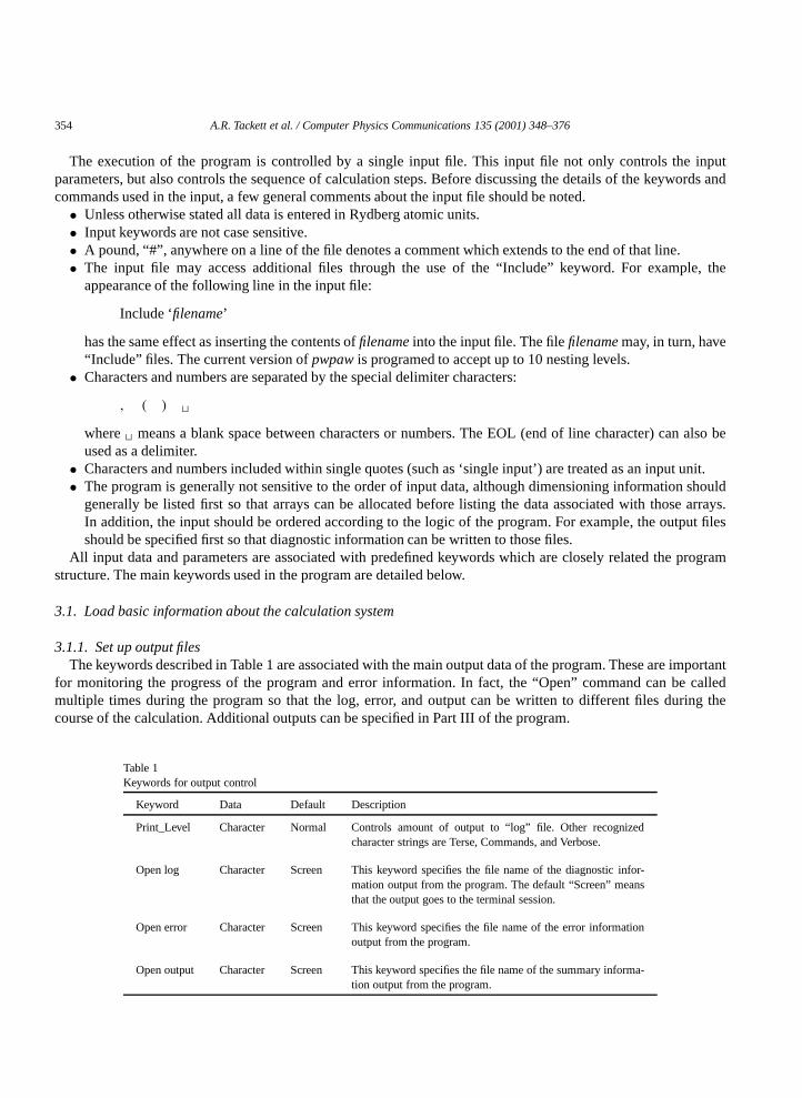
3.1.1. Set up output filesThe keywords described in Table 1 are associated with the main output data of the program. These are important

for monitoring the progress of the program and error information. In fact, the “Open” command can be calledmultiple times during the program so that the log, error, and output can be written to different files during thecourse of the calculation. Additional outputs can be specified in Part III of the program.

Table 1Keywords for output control

Keyword Data Default Description

Print_Level Character Normal Controls amount of output to “log” file. Other recognizedcharacter strings are Terse, Commands, and Verbose.

Open log Character Screen This keyword specifies the file name of the diagnostic infor-mation output from the program. The default “Screen” meansthat the output goes to the terminal session.

Open error Character Screen This keyword specifies the file name of the error informationoutput from the program.

Open output Character Screen This keyword specifies the file name of the summary informa-tion output from the program.


Table 2Keywords for main data structures of program


Max_AtomTypes Integer (none) The maximum number of different types of atoms that will be used in thiscalculation. This keyword must come before any atomic data can be loaded.

Max_SpecificAtoms Integer (none) The maximum total number of atoms that will be used in this calculation.This keyword must come before any atomic data can be loaded.

MinPsi Integer 1.25×Nv Calculated default is 25% larger than the total number of valence electronsper unit cell (Nv). This number controls the number of eigenstates perk-point that will be calculated. For SCF calculations this number should belarger than1

2 the number of valence electrons per unit cell. For density ofstates or band structure calculations, it should be larger than the total numberof bands desired.

Max_TotalPsi Integer 2×MinPsi This number should be larger than MinPsi and controls the size of thewavefunction arrays.

Psi_Memory Real 40 The value represents the number of megabytes available for storing wavefunction coefficientsAnk(G).

Proj_Memory Real 40 The value represents the number of megabytes available for storing theprojector functionspa

i.

Bloch_Memory Real 5 The value represents the number of megabytes available for storing phasefactors of the form eiG·Ra .

Ylm_Memory Real 5 The value represents the number of megabytes available for storing sphericalharmonic valuesYlm(k + G) which are needed for calculating projectorfunctions.

3.1.2. Set up data structuresThe keywords described in Table 2 must be listed near the beginning of the input file so that data structures can

be set up and arrays allocated for additional data input.

3.1.3. Define crystal and set plane-wave cutoffsThe keyword “SuperCell” is associated with the definition of the unit cell lattice parameters, the crystal

symmetry, and the Brillouin zone sampling parameters.

SuperCellScalexsA Ax Ay AzB Bx By BzC Cx Cy Cz

Clone_CellmA mB mC

Include ‘crystal-symmetry.file’Include ‘k-point-list.file’


BZ_Method GAUSSGauss_Widthσ

End

Here, the keyword “Scale” is optional and can be used to set a scale factor (xs) for the lattice vectors. The labels“A”, “B”, and “C” represent three independent vectors which define the unit cell of the calculation. The valueslisted after each are the Cartesian components of those vectors in units of Bohr, optionally scaled by the valueof xs . The keyword “Clone_Cell” is optional and can be used to enlarge the unit cell of the calculation so thatthe lattice vectors of the supercell become(1 +mA)A, (1+mB)B, and(1+mC)C. The program was written for{mA,mB,mc} being positive integers.

The Include ‘crystal-symmetry.file’ statement or its contents as described below can be included if the crystalhas non-trivial symmetry (that is a space group of orderNSG greater than 1). The crystal symmetry is defined bythe rotation matricesRi and non-primitive translation vectorsτ which take a general point within the unit cellrand map it to a physically equivalent pointr′ according to

r′ =Rir + τ i . (22)

The contents of the “crystal-symmetry.file” take the form:

Rot_SizeNSG

Matrix i

Rixx Ri

xy Rixz

Riyx Ri

yy Riyz

Rizx Ri

zy Rizz

EndTranslationi f iA f

iB f

iC

...

Here the indexi goes from 1 toNSG, Rijk denotes elements of the rotation matrixRi in a Cartesian representation,

and the translation vector is represented in fractional units of the primitive translation vectors according toτ i ≡ f iAA + f iBB + f iCC. Alternatively, the inclusion of the keyword ‘AUTO_SYMMETRY’ calculates the crystalsymmetry from the lattice translation and atomic position data. If this keyword is present, the program recalculatesthe symmetry if the atoms are moved within the run.

The Include ‘k-point-list.file’ statement or its contents as described below specifies thek-point sampling in thefollowing form.

K-Points_ListNkfGA fGB fGC Wk...

End

Here, each of theNk k-points is specified in fractional units of the primitive reciprocal lattice vectors according tok ≡ fGAGA + fGBGB + fGCGC . The numberWk represents the corresponding relative weighting factor which isnormalized to unity within the program. The remaining keywords and constants in this section relate to the methodof Brillouin zone integration. In the example, ‘BZ_Method GAUSS’ means that a Gaussian smoothing function


was used following the approach of Fu and Ho [19], so that the occupancy factor which appears in the calculationof the electron density (Eqs. (4) and (5)) is approximated by

fnk = Wk∑k′ Wk′

{1+ erf

(EF −Enk

σ

)}, (23)

whereσ is a smoothing parameter set by the input keyword and constant ‘Gauss_Widthσ ’ andEF is the Fermilevel which determined from the total number of valence electrons per unit cellNv , by solving the transcendentalequation [20]∑

nk

fnk =Nv. (24)

Other Brillouin zone schemes could easily be implemented into the code. A short program,genkpoints, to reada pwpaw input file containing the primitive lattice vectors and symmetry operations and to interactively generateuniformly distributed inequivalentk-points (genkpoints is included in the package).

The keyword “PlaneWave_Cutoffs” is used to set the range of reciprocal lattice vectors used in the calculationaccording to the format shown in the following example.

PlaneWave_CutoffsGcut_LOWvalueGcut_HIGHvalueGcut_PROJvalue

End

Here, the value of Gcut_LOW determines the truncation of the plane wave expansion of the wavefunction inEq. (1), and Gcut_HIGH determines the truncation of the plane wave expansion of the density in Eq. (4). Thelarger cutoff is also used to construct the fast-Fourier-transform grid to perform the evaluation of the pseudo-density efficiently [21]. The keyword ‘Gcut_PROJ’ is optional. If it is present, the value determines the accuracyof the evaluation of the matrix elements of the smooth wave functions and the projectors〈pai |Ψnk〉 if the additionalkeyword “Real_Space_Projectors” is used (see Table 3).

3.1.4. Load atom information and set electron countFor each atomic species of the calculation, atomic projector and basis functions and associated matrix elements

are needed. These are generated by theatompaw program in a file [atomic symbol].atomicdata. The format for thisfile is described in Ref. [8] and can be included in thepwpaw input using the format

Include ‘[atomic symbol].atomicdata’

for each atom.After the atomic data has been loaded, the electron count is established by specifying the initial configuration

in terms of a linear combination of atomic orbital (LCAO) basis. This information is also used to begin the firstcalculation of a new system. The following keywords are used.

AtomType_Occupancy [atomic symbol]Orbitals_SizeNLCAOValence_Orbitalsi1 i2 . . . iNLCAO

Valence_Occupancyνi1 νi2 . . . νiNLCAO

RS_Scalef ar

End


The keyword ‘AtomType_Occupancy’ takes an atomic symbol argument which must correspond to the atomicsymbol defined in the [atomic symbol].atomicdata file. The keyword ‘Orbitals_Size’ specifies the number of LCAOorbitals which will follow in the specification. The keyword ‘Valence_Orbitals’ is followed by a list of thei indicescorresponding to theφani li (r) radial basis functions to be included in the initial configuration. In order to start thecalculation with a set of reasonable LCAO functions, it is prudent to include basis functions which correspond tobound atomic states only. The keyword ‘Valence_Occupancy’ is followed by a list of the initial occupanciesνaiof the LCAO bands. Some of the occupancies may be zero, but the sum of all the occupancies and over all atomsshould correspond to the total number of electrons per unit cell

∑ai ν

ai =Nv . The keyword “RS_Scale” is optional.

If the “Real_Space_Projectors” keyword is present (see Section 3 below), the cutoff radius for the grid evaluationof 〈pai |Ψnk〉 is set to bef ar r

ac . By default,f ar = 1.5.

The initial atomic positions can also be specified after the atomic data has been loaded. There are two possibleformats for specifying the atomic positions: fractional coordinates or Cartesian coordinates. For the former, theatomic positions are given in terms of the lattice vectors according toRa = f aAA + f aBB + f aCC and specified asfollows.

Atom_List FRAC_POSITION[Specific atom label] [Atomic symbol]f aA f

aB f

aC

...

End

Alternatively, the specification in terms of Cartesian coordinates can be given as follows.

Atom_List CART_POSITION[Specific atom label] [Atomic symbol]Rax R

ay R

az

...

End

In this case, the atomic position components(Rax ,Ray ,R

az ) are given in Bohr units. In either case, the atomic

positions must be consistent with the symmetry of the crystal in the sense that for each atomic positionRa andeach space group element(Ri , τ i),

Rb = RiRa + τ i, (25)

whereRb corresponds to the position of the same or an equivalent atom in the unit cell. The program checksthat (25) is satisfied within a tolerance of 10−6 Bohr units. If the keyword “Clone_Cell” is set as describedabove, then additional atomic positions are generated and each is given a “Specific atom label” of the form[Specific atom label]_uvw, where 0� u�mA, 0� v �mB , and 0�w �mC .

3.1.5. Set calculation optionsTable 3 lists some of the keywords which are used to control the calculations and execution parameters for the

program.The parameters which control the SCF cycle are included in Table 4. Following the suggestions of Eyert [15], we

use the convergence acceleration algorithm of Anderson [16] which uses a mixing parameter to control the stabilityof the iterations. In order to minimize the possible effects of charge slashing [11], two mixing parameters are given.When the change in the cohesive energy for successive iterations, is small, the first parameter is used. When thechange is larger than the value specified with the “Mix_SecondValue” keyword, the second mixing parameteris used. Finally, the keyword “Filter_Potential” and parameter “V_Smooth_Width” implements the algorithm ofWang and Zunger [22] for reducing large Fourier components to the effective potentialveff.


Table 3Keywords for setting calculation options


XC_Type Character XC_Perdew This keyword controls the functional form of the exchange-correlation functional. The currently implemented case is areXC_Perdew [10] which is consistent with exchange-correlationfunctional form used in the atom programatompaw.

Forces_always_calc_H (none) Not present The presence of this keyword ensures that theDaij matrix elementsare recalculated when the forces are evaluated. If the keyword isnot present in the input file, the stored matrix elements are used forevaluating the forces.

Anchor Character Not present The presence of this keyword sets the specific atom indicated withthe character data value acts as an anchor to the system in thegeometry optimization or in molecular dynamics.

Freeze Character Not present The presence of this keyword sets a calculational flag to ensurethat the specific atom indicated with the character data value willnot move in the geometry optimization or in molecular dynamics.Unlike the “Anchor” keyword, more than one atom can be fixed inthe calculation with the “Freeze” keyword.

Real_Space_Projectors (none) Not present The presence of this keyword specifies that the evaluations of thematrix elements〈pa

j|Ψnk〉 will be evaluated on a real space grid.

The associated keyword “Gcut_Proj” determines the grid spac-ing from the associated fast-Fourier-transform and the keyword“RS_Scale” determines the effective integration radius. This formevaluates the matrix elements much faster than the Fourier spacesum with reasonable accuracy for large unit cells.

No_O_Eigenvalues (none) Not present The presence of this keyword means that the generalized eigenvalueproblem is solved by factorizing the overlap matrix, rather thanthe default algorithm which diagonalizes the overlap matrix. Ifthis procedure returns an error code, the program uses the defaultalgorithm.

Overlap_Tol Real 10−11 This parameter controls the minimum eigenvalue of the overlapmatrix which is used to solve the generalized eigenvalue problem.

3.2. Initialize calculation

The keyword ‘Initialize_System’ is used to call a series of subroutines which use the loaded data to prepare thedata structures which will be used in the program. This initialization step is then followed by the preparation ofthe initial smooth wave functions by one of the following three possibilities. The default is a call to the subroutineCalcLCAO, which is the default and needs no additional keywords. Alternatively, the results of a previous run ofthe program can be loaded by using the following form.

Load_SolutionRestartFilename

The binary file, ‘RestartFilename’, generated by the command ‘Store_Solution binary’ described below in aprevious run of the program which may have had different plane wave cutoff parameters or different numbersof wave functions. Alternatively, the keyword ‘Random_Guess’ can be used to use a random number generator toinitialize the smooth wave functions.


Table 4Keywords for setting parameters which control the convergence of the SCF cycle


Mix_V, Mix_Veff,or Mix_Density

(none) Mix_Veff This keyword controls how the SCF cycles are updated using theAnderson mixing algorithm discussed above using the Coulombpotential corresponding ton+ n, usingveff, or usingn, respectively.

V_NewMix Real Real 0.5 0.25 Determines the initial value of the Anderson mixing procedure forthe potential or density updating mode in the SCF cycle. If thesevalues are greater or equal to 0.9999, no mixing is done.

Dij_NewMix Real Real 1.0 1.0 Determines the initial value of the Anderson mixing procedure forupdating theDa

ijmatrix elements in the SCF cycle. If these values

are greater or equal to 0.9999, no mixing is done.

Mix_SecondValue Real 0.2 This parameter determines when to switch Anderson mixingparameters from the first (fractional change in cohesive energy isless than parameter value) to the second.

Mix_Size Integer 5 The parameter determines the maximum number of update dataused in the Anderson mixing algorithm.

Filter_Potential (none) Not present This option removes large Fourier components of the potentialveff.

V_Smooth_Width Real 0.0 If the Filter_Potential option has been chosen, this parametercontrols the rate of smoothing of the potentialveff in Fourier space,following the approach of Wang and Zunger [22]. The value ofthis parameter corresponds to 1− β defined in Appendix A of thereference.

3.3. Keyword command control of program

3.3.1. Self-consistent electronic structureFor self-consistent field (SCF) calculations at fixed atomic positions, the keyword command structure is as

follows.

Relax ChargeSCFIter MeritTol

In this case,SCFIter denotes the maximum number of iteration steps, described in Section 2.4, that are carried outbefore the program stops. The parameterMeritTol is also defined in Section 2.4.

3.3.2. Store solutionsIn order to store the wave functions for later use by the program, the following keyword command can be used.

Store_solution

binary

textRestartFilename

The file RestartFilename contains information about the reciprocal lattice cutoffs and thek-point sampling inaddition toEnk, fnk, and{Ank(G)} for each calculated state. The “binary” form means that the file is stored withunformatted output. In order to transfer data to another operating system, the “text” (formatted) form can be usedinstead.

For calculating the band structure, the self-consistent local and non-local potential termsveff andDaij are needed.These can be saved or retrieved by using the keywords


Store_Hamiltonian

or

Load_Hamiltonian

respectively.

3.3.3. Calculate forces or energyIn order to calculate the forces on atoms after an SCF calculation, the following keyword command can be used.

Calculate ForcesForceOutput

Here, the parameterForceOutput resets the file name for the output of atomic position and force information. Thedefault name is “paw.forces”. The program is written to append the force output to the end of any existing outputfile. The forces reported are those calculated from Eq. (18).

In order to calculate the cohesive energy and output the result to the “Output_Unit”, the command “CalculateEnergy” can be used.

3.3.4. Geometry optimizationFor calculations which optimize the cohesive energy with respect to the atomic positions on the Born–

Oppenheimer surface, the keyword command structure is as follows.

Relax GeometryMaxSteps Output SCFIter MeritTol ForceTol MaxMove

In this mode, the program performs an SCF calculation at “MaxSteps” different geometries, or less. For each SCFcalculation, as in the “Relax Charge” mode described above, a maximum of “SCFIter” iterations are allowed toachieve the convergence of the cohesive energy within the allowance of the “MeritTol ” parameter. At the end

of each SCF calculation, the forces on each atom are calculated according to Eq. (18). If√∑

a |Fa|2 is larger

than “ForceTol ”, the atoms are moved to new positions in the direction ofFa . The parameterMaxMove controlsthe magnitude of the move. Ideally, this magnitude should be small enough so that the SCF iteration in the newgeometry can use the wavefunctions of the previous geometry for a rapidly convergent calculation. The parameter“Output ” can either list a file name for saving wavefunction information at each geometry step or can be set to“NULL” indicating that the wavefunction is not to be saved. After each force calculation, the position and forceinformation is appended to the force output file which can be renamed by the “Calculate ForcesForceOutput ”command as explained above.

3.3.5. Calculation of the density of states, partial density of states, electron densities, or band structureThe densities of states or electron densities for selected states can be calculated after any SCF step. The

program is used in a ‘bandstructure’ mode which takes converged results forveff andDaij and performs iterativediagonalization to solve the generalized eigenvalue equations (12) using the same block Davidson algorithmdiscussed in Section 2.4. While for the SCF calculation, only occupied states affect the convergence test, for the‘bandstructure’ mode of the program, all states with Kohn–Sham eigenvaluesEnk � EigenMax are included in thedefinition of the merit function:

Eαmerit ≡∑

Enk�EigenMax

|Enk|. (26)

Therefore, the band merit function is defined to be

BandMerit ≡ ∣∣Eα+1merit −Eαmerit

∣∣. (27)

The value ofEigenMax can be set with a command of the following form.


Set_EigenMaxEigenMax

In conjunction with setting the value ofEigenMax, it is necessary to make sure that the data structures for thewavefunctions are dimensioned large enough to accommodate the additional states. This is controlled in the firstsection of the program, as described in Section 3.1.2 through the ‘MinPsi’ and ‘Max_TotalPsi’ parameters.

The commands for calculating the density of states are given by the following.

Calculate DOSDOSFilename DOSIter DOSTol

Here, DOSFilename specifies the output file name for the density of states information,DOSIter determineshow many iterative diagonalization steps are allowed, andDOSTol denotes the maximum value ofBandMeritat convergence. The commands for calculating the partial density of states are given by the following.

Calculate PDOSPDOSFilename P PDOSIter PDOSTolATOM [Specific atom label] S

...

label fA fB fC S...

P sites

End

In the PDOS mode of the program, the chargeCp

nk associated with each eigenstatenk of the system within eachof P spheres is written out to the filePDOSFilename. The number of iterationsPDOSIter and the convergencetolerancePDOSTol are exactly analogous to the DOS case. For each of theP spheres, a radiusS is specified. Thekeyword ATOM indicates that this sphere is associated with an atomic site with the given [Specific atom label]. Inthis case,S � rac . Any other label can be used to specify a sphere centered at the locationfAA + fBB + fCC.

The DOSFilename and PDOSFilename can be processed by the short interactive programpreparepdos togenerate the density of states from the Gaussian smearing function [19]. The partial density of states associatedwith thepth sphere can be calculated from:

Np(E)= 2√πσ(

∑k′ Wk′)

∑nk

Cp

nkWk e−(E−Enk)2/σ2

, (28)

whereWk denotes thek-point weight factor defined earlier. In this expression, theδ-function in energy forevaluating the density of states has been replaced by a Gaussian function of widthσ which need not be the sameas that used (Eq. (23)) for the SCF calculations.2 The same form can be used for the density of states calculationsby settingCpnk ≡ 1.

The commands for calculating electron densities corresponding toNd selected energy ranges is given by thefollowing.

Calculate Partial_DensitiesNd PDIter PDtol

OccFlag PDFilename Emin Emax

...

Nd partial densities

End

2 An advantage of this approach is that it avoids numerical spikes in the evaluation of the density of states and therefore facilitates comparison,as shown, for example, in Ref. [5] in the comparison of the density of states for CaMoO4 calculated using the PAW and LAPW methods.


HerePDIter andPDtol represent the number of iterative diagonalization steps and convergence tolerance, similarto those variables in the density of states calculations. The parameterOccFlag can either be “OCC”, meaningthat the occupancy factorsfnk calculated in the SCF step from Eq. (23) should be used, or “NOT”, meaningthat the occupancy should be calculated from the Brillouin zone weight factors, alone, assuming that the bandsare fully occupied. That is, calculatingfnk by using Eq. (23) withEF → ∞. For each energy range, whereEmin � Enk � Emax, the partial densitynd(r) can be constructed from a knowledge of the Fourier coefficientsof the partial pseudo-density

nd (r)=∑

Emin�Enk�Emax

fnk∣∣Ψnk(r)

∣∣2 = 1

V∑

G

¯nd(G)eiG·r, (29)

and the partial projected occupation coefficients

Wadij ≡

∑Emin�Enk�Emax

fnk⟨Ψnk

∣∣pai ⟩⟨paj ∣∣Ψnk⟩. (30)

The Fourier coefficientsnd(G) and partial projected occupation coefficientsWadij are calculated and written to the

file namedPDFilename.In order to construct a bandstructure plot, it is necessary to determine the energy eigenvaluesEnk for a set

of wave vectors that are generally different from those used during the SCF step. After an SCF calculation, aLoad_Solution keyword, or a Load_Hamiltonian keyword, the following command can be used:

Calculate Band_StructureBandfilename BandIter BandTol

HereBandfilename denotes the name of an input file which contains the list ofk-points. The band structure outputis written to a file named “Bandfilename.band”. The number of iterations allowed for eigenvalue solver is specifiedby the integerBandIter andBandTol specifies the convergence tolerance of the merit function (27). The format oftheBandfilename input file is as follows.

MaxbandsfGA fGB fGC...

HereMaxbands specifies the maximum number of bands that are expected for any of thek-points. This parametersupersedes the value ofMax_TotalPsi and it should be consistent with the choice ofEigenMax. Thek-points arelisted in fractional units of the primitive reciprocal lattice vectors. The program processes each newk-point untilreaching the end of the file. The output file listsk andEnk for each band. A simple programbandplot can then beused to convert the fractional wave vectors into a a scalar length along specified directions in the Brillouin Zonefor constructing a band diagram.

3.3.6. Contour plots of the electron densityThe program is constructed to prepare data for use with IBM’s Data Explorer software. The output can be easily

modified for use with other plotting software. Both 2- and 3-dimensional plots can be constructed for each of thepartial density filesPDFilename. The keyword commands are designed to first setup the parameters of the plottingarea or volume. For the 3-dimensional plots, the setup parameters are given in the following form.

Plot 3DSetupX Xx Xy XzY Yx Yy YzZ Zx Zy Zz


O Ox Oy OzGrid Nx Ny NzPlotName PlotFilenameBond b

BondTol u

End

Here the keywords “X”, “Y”, “Z”, and “O” are each followed by 3 Cartesian coordinates in Bohr units, whichspecify the 3 orthogonal vectorsX–O, Y–O, andZ–O which define the plotting volume. The keyword “Grid”specifies the uniform grid on which densityn(r) will be evaluated within the plotting volume. The keyword“PlotName” specifies the prefix of the output plotting files used with the “Plot 3datom” keyword described below.The keywords “Bond” and “BondTol” are optional keywords which specify stick model bonds that can be drawn.Here,b specifies the largest distance between two atoms for which a bond will be drawn. The parameteru specifiesthe fractional bond length to plotting cell length ratio which allows atoms outside the plotting cell to be includedin the ball and stick plot.

For 2-dimensional plots, the setup parameters are given in a similar form.

Plot 2DSetupX Xx Xy XzY Yx Yy YzO Ox Oy OzGrid Nx NyPlotName PlotFilename

End

Once these parameters have been set up, the plots can be constructed using

Plot 3d-densityPDFilename

or

Plot 2d-densityPDFilename

for the 3- or 2-dimensional plots, respectively. The 3-dimensional case additionally outputs information to constructa ball and stick model for each plot. To output only the ball and stick model information, the following keywordcommand can be used.

Plot 3datom

Output is also generated in a format which can be viewed using the program XCrySDen [23].

4. Sample programs

4.1. CaO

This example was discussed in Ref. [8]. The input file to calculate the SCF cycle for this material structure atthe lattice constanta = 4.7 Å for the projector and basis set we labeled“sinc”,rc=1.4(x2) is given as follows.


## Input file for CaO at lattice constant = 4.7 A#Print_Level VERBOSEopen Log ’CaO1.log’ # Set output filesOpen Error ’CaO1.error’Open output ’CaO1.out’

Max_AtomTypes 2MAx_Specific_Atoms 2Max_TotalPsi 18MinPsi 16

Psi_Memory 200Proj_Memory 100Ylm_Memory 100Bloch_Memory 100

SuperCell # Define the crystalScale 1.889725989A ( 2.3500000, 2.3500000, 0.0000000)B ( 2.3500000, 0.0000000, 2.3500000)C ( 0.0000000, 2.3500000, 2.3500000)

Include ’CaO.crystal-symmetry’Include ’CaO.k-point-list’Gauss_Width 0.001BZ_Method GAUSS

End

PlaneWave_CutoffsGcut_LOW 10Gcut_HIGH 12

End

Include ’../atom/O/sinc4rc1.4/O.atomicdata’Include ’../atom/Ca/Ca.atomicdata’

AtomType_Occupancy OOrbitals_Size 2Valence_Orbitals 1 3Valence_occupancy 2 4

End

AtomType_Occupancy CaOrbitals_Size 3Valence_Orbitals 1 2 3Valence_occupancy 2 2 6

End

Atom_List Frac_PositionO O (0.5,0.5,0.5)


Ca Ca (0.0,0.0,0.0)End

XC_Type Perdew-WangFORCES_ALWAYS_CALC_HMix_VeffV_NewMix 0.2 .1Dij_NewMix 0.2 .1Mix_SecondValue .2

Initialize_SystemLoad_Solution ’CaO.pwfn1a’

Relax charge 30 1.E-7Store_Solution binary ’CaO.pwfn1’Quit

In this example, the “Include” files are in different directories, and are specified using the Unix directoryconventions. The list ofk-points file has the form:

K-Points_List 100.1250000000000000 0.1250000000000000 0.1250000000000000 2.000000.3750000000000000 0.1250000000000000 0.1250000000000000 6.00000

-0.3750000000000000 0.1250000000000000 0.1250000000000000 6.00000-0.1250000000000000 0.1250000000000000 0.1250000000000000 6.000000.3750000000000000 0.3750000000000000 0.1250000000000000 6.00000

-0.3750000000000000 0.3750000000000000 0.1250000000000000 12.00000-0.1250000000000000 0.3750000000000000 0.1250000000000000 12.00000-0.3750000000000000 -0.3750000000000000 0.1250000000000000 6.000000.3750000000000000 0.3750000000000000 0.3750000000000000 2.00000

-0.3750000000000000 0.3750000000000000 0.3750000000000000 6.00000End

The calculation is restarted with the results of a previous run at smaller plane wave cutoffs which was storedin the file ‘CaO.pwfn1a’. The results of the calculation are shown in Fig. 2. In this case, the restarted calculationconverged in 8 iterations.

# SCF results generated on date 05/16/2000, 10:20:57.375RelaxElectrons: Converged in 8 iterations with a final Energy error of

0.487360836132211261E-07RelaxElectrons: Cohesive Energy: 1.05488501097457288RelaxElectrons: # iterations : 8 / 50RelaxElectrons: Tolerance : 0.487360836132211261E-07 / 0.999999999999999955E-07# Current Fractional Positions#Atom_List FRAC_POSITION# O O 5.00000E-01 5.00000E-01 5.00000E-01# Ca Ca 0.00000E+00 0.00000E+00 0.00000E+00Energies for cluster 1 (DiskRec, Energy, Occ, Kpnt) * Size: 110 * -2.36959106909795603 * 0.625000000000000000E-01 * 1Energies for cluster 2 (DiskRec, Energy, Occ, Kpnt) * Size: 311 * -1.02263048301959358 * 0.625000000000000000E-01 * 112 * -1.00683529157566687 * 0.625000000000000000E-01 * 113 * -1.00683529146213879 * 0.625000000000000000E-01 * 1

Fig. 2. Output file for CaO example.


Energies for cluster 3 (DiskRec, Energy, Occ, Kpnt) * Size: 114 * -0.773623079657166146 * 0.625000000000000000E-01 * 1Energies for cluster 4 (DiskRec, Energy, Occ, Kpnt) * Size: 315 * 0.283676485941666723 * 0.625000000000000000E-01 * 116 * 0.307602676693226107 * 0.625000000000000000E-01 * 117 * 0.307602677770904331 * 0.625000000000000000E-01 * 1Energies for cluster 5 (DiskRec, Energy, Occ, Kpnt) * Size: 418 * 0.717838616819526432 * 0.000000000000000000E+00 * 119 * 0.767500661111773175 * 0.000000000000000000E+00 * 120 * 0.790069906475341477 * 0.000000000000000000E+00 * 121 * 0.790069941281033139 * 0.000000000000000000E+00 * 1Energies for cluster 6 (DiskRec, Energy, Occ, Kpnt) * Size: 222 * 0.911792965109302744 * 0.000000000000000000E+00 * 123 * 0.911793031667607501 * 0.000000000000000000E+00 * 1Energies for cluster 7 (DiskRec, Energy, Occ, Kpnt) * Size: 124 * 1.45523265404801361 * 0.000000000000000000E+00 * 1Energies for cluster 8 (DiskRec, Energy, Occ, Kpnt) * Size: 325 * 1.89509402235662949 * 0.000000000000000000E+00 * 126 * 1.92648052021326599 * 0.000000000000000000E+00 * 127 * 1.92648060884543959 * 0.000000000000000000E+00 * 1Energies for cluster 9 (DiskRec, Energy, Occ, Kpnt) * Size: 128 * -2.36466364750619773 * 0.187500000000000000 * 2Energies for cluster 10 (DiskRec, Energy, Occ, Kpnt) * Size: 329 * -1.06484636812383981 * 0.187500000000000000 * 230 * -1.01599534858570451 * 0.187500000000000000 * 231 * -1.00799009742767831 * 0.187500000000000000 * 2Energies for cluster 11 (DiskRec, Energy, Occ, Kpnt) * Size: 132 * -0.727530323924740041 * 0.187500000000000000 * 2Energies for cluster 12 (DiskRec, Energy, Occ, Kpnt) * Size: 333 * 0.181914652254444420 * 0.187500000000000000 * 234 * 0.251387221971676345 * 0.187500000000000000 * 235 * 0.274027709194861913 * 0.187500000000000000 * 2Energies for cluster 13 (DiskRec, Energy, Occ, Kpnt) * Size: 136 * 0.768292789192570935 * 0.000000000000000000E+00 * 2

...180 * 1.35040430531786848 * 0.000000000000000000E+00 * 10181 * 1.41834909986961488 * 0.000000000000000000E+00 * 10Energies for cluster 107 (DiskRec, Energy, Occ, Kpnt) * Size: 1182 * 1.64971133783488244 * 0.000000000000000000E+00 * 10Exiting PAW program

Fig. 2. Continued.

4.2. Diamond

This example shows a SCF calculation for diamond, followed by a calculation of the band structure along theX–Γ –L directions. The input file is given as follows.

## Input file for diamond#open Log ’diamond.log’ # Set output filesOpen Error ’diamond.error’Open output ’diamond.out’

Max_AtomTypes 1MAx_Specific_Atoms 2


Max_TotalPsi 20MinPsi 4Psi_Memory 200Proj_Memory 100Ylm_Memory 100Bloch_Memory 100

SuperCell # Define the crystalA (3.35237480000000000, 3.35237480000000000, 0.00000000000000000)B (0.00000000000000000, 3.35237480000000000, 3.35237480000000000)C (3.35237480000000000, 0.00000000000000000, 3.35237480000000000)

Include ’diamond.k-point-list’Include ’diamond.crystal-symmetry’

Gauss_Width 0.001BZ_Method GAUSS

End


End

Include ’../../atom/C/C.atomicdata’

AtomType_Occupancy COrbitals_Size 2Valence_Orbitals 1 2Valence_occupancy 1 3

End

Atom_List Frac_PositionC1 C ( 0.125, 0.125, 0.125)C2 C (-0.125,-0.125,-0.125)

End

XC_Type Perdew-WangFORCES_ALWAYS_CALC_HMix_VeffV_NewMix 1.0 0.2Dij_NewMix 1.0 0.2Mix_SecondValue 0.2

Initialize_System

Relax charge 30 1.0E-6Store_Solution binary ’diamond.wfn1.binary’

Set_Eigenmax 4Calculate Band_structure diamondXL 40 1.E-5Quit


## Input file for Ti2Nb6O12 using structural data of Katya Anokhina#open Log ’paw.log’ # Set output filesOpen Error ’paw.error’Open output ’paw.out’

Max_AtomTypes 3MAx_Specific_Atoms 20

Max_TotalPsi 120MinPsi 115

Psi_Memory 200Proj_Memory 100Ylm_Memory 100Bloch_Memory 100

SuperCell # Define the crystalA (8.658880719, 0, 9.092038650)B (-4.329440361, 7.498810670, 9.092038650)C (-4.329440361, -7.498810670, 9.092038650)

Include ’tinbo.k-point-list’Include ’tinbo.crystal-symmetry’

Gauss_Width 0.001BZ_Method GAUSS

End


End

Include ’O.atomicdata’Include ’Nb.atomicdata’Include ’Ti.atomicdata’

AtomType_Occupancy OOrbitals_Size 2Valence_Orbitals 1 3Valence_occupancy 2 4

EndAtomType_Occupancy Nb

Orbitals_Size 4Valence_Orbitals 1 2 3 5Valence_occupancy 2 1 6 4

EndAtomType_Occupancy Ti

Orbitals_Size 4Valence_Orbitals 1 2 3 5Valence_occupancy 2 2 6 2

End

Fig. 3. Input file for Ti2Nb6O12 SCF calculation.


Atom_List Cart_Position01 O .3571788298, -2.899790086, 4.72695089402 O -.3571788298, 2.899790086, -4.72695089403 O 2.332702467, 1.759220983, 4.72695089404 O -2.332702467, -1.759220983, -4.72695089405 O -2.689881296, 1.140569103, 4.72695089406 O 2.689881296, -1.140569103, -4.72695089407 O -3.339297351, 4.512034380, -.0163656695708 O 3.339297351, -4.512034380, .0163656695709 O -2.237887723, -5.147933525, -.01636566957010 O 2.237887723, 5.147933525, .01636566957011 O 5.577185072, .6358991448, -.01636566957012 O -5.577185072, -.6358991448, .01636566957Nb1 Nb 2.823661003, -1.303293294, 2.127537044Nb2 Nb -2.823661003, 1.303293294, -2.127537044Nb3 Nb -.2831453995, 3.097008807, 2.127537044Nb4 Nb .2831453995, -3.097008807, -2.127537044Nb5 Nb -2.540515603, -1.793715512, 2.127537044Nb6 Nb 2.540515603, 1.793715512, -2.127537044Ti1 Ti 0, 0, -7.474564973Ti2 Ti 0, 0, 7.474564973End

XC_Type Perdew-WangFORCES_ALWAYS_CALC_HMix_VeffV_NewMix 0.20 .1Dij_NewMix 1.0 0.2Mix_SecondValue 0.2

Initialize_System

Relax charge 80 1.0E-7Calculate Forces ’tinbo.force1’Store_Solution binary ’tinbo.pwfn1’

Quit

Fig. 3. Continued.

In this case, the wavefunctions generated during the SCF step are used to generate an initial guess for the firstk-point of the band calculation. Thek-point file, named “diamondXL” has the following contents:

20 # maximum number of bands per k-point0.5 0.5 0 # X point0.4 0.4 00.3 0.3 00.2 0.2 00.1 0.1 00 0 0 # Gamma point0.1 0.1 0.10.2 0.2 0.20.3 0.3 0.30.4 0.4 0.40.5 0.5 0.5 # L point


K-Points_List 60.1666666666666667 0.1666666666666667 0.1666666666666667 2.000000.4999999999999999 0.1666666666666667 0.1666666666666667 6.00000

-0.1666666666666667 0.1666666666666667 0.1666666666666667 6.000000.4999999999999999 0.4999999999999999 0.1666666666666667 6.00000

-0.1666666666666667 0.4999999999999999 0.1666666666666667 6.000000.4999999999999999 0.4999999999999999 0.4999999999999999 1.00000

End

Fig. 4.k-points file for Ti2Nb6O12.

Rot_Size 6

Matrix 11 0 00 1 00 0 1

EndTranslation 1 0.000000000000E+00 0.000000000000E+00 0.000000000000E+00

Matrix 2-1 0 00 -1 00 0 -1


Matrix 3-0.5 .86602540378443864675 0-.86602540378443864675 -0.5 00 0 1


Matrix 4-0.5 -0.86602540378443864675 0.86602540378443864675 -0.5 00 0 1


Matrix 50.5 -0.86602540378443864675 0.86602540378443864675 0.5 00 0 -1


Matrix 60.5 0.86602540378443864675 0

-.86602540378443864675 0.5 00 0 -1


Fig. 5. Symmetry file for Ti2Nb6O12.


.

.

.


.

.

.

Initialize_SystemLoad_Solution ’tinbo.pwfn1’

Set_EigenMax 2.0Calculate PDOS ’tinbo.pdos’ 20 40 1.e-6ATOM O1 1.51ATOM O2 1.51ATOM O3 1.51ATOM O4 1.51ATOM O5 1.51ATOM O6 1.51ATOM O7 1.51ATOM O8 1.51ATOM O9 1.51ATOM O10 1.51ATOM O11 1.51ATOM O12 1.51ATOM Nb1 2.21ATOM Nb2 2.21ATOM Nb3 2.21ATOM Nb4 2.21ATOM Nb5 2.21ATOM Nb6 2.21ATOM Ti1 2.21ATOM Ti2 2.21

End

Store_Solutions ’tinbo.dos.pwfn1’Quit

Fig. 6. Modifications to input file (Fig. 3) needed for calculating partial densities of states if Ti2Nb6O12.

4.3. Ti2Nb6O12

A more strenuous demonstration of the program was suggested by colleagues from the Chemistry department.The compound Ti2Nb6O12 is one of a series of transition metal oxides which are under investigation for theirstructural properties [24]. It crystallizes in a rhombohedral structure with one formula unit per unit cell. The inputfile, the k-points file, and crystal symmetry files are shown in Figs. 3, 4, and 5, respectively. In this case, thesymmetry group has a total of 6 operations including inversion and a rotation of±120◦ about thez-axis. Theatom centered basis and projector functions were calculated using theatompaw code [8] using the “sinc” shapefunction with the basis choice andrac values listed in Table 5. This material has two transition metals with verysimilar electronegativities, so that the charge transfer between the two is delicately balanced. After the calculationconverged, the partial densities of states where calculated using the modified input file shown in Fig. 6. Afterprocessing the output (which is in this case written to a file named “tinbo.pdos.pdosout”) using the interactiveprogrampreparepdos, the resultant partial density of states are obtained as shown in Fig. 6. In this case, the resultsfor the individual atoms of each type were averaged to form 3 partial density of states curves — for Ti, Nb, and O.Here we see that this material is a semiconductor with a small band gap. The O states are completely filled and the


Table 5Atomic basis parameters used for Ti2Nb6O12 calculations

Atom {ni li } rac (Bohr)

Ti 3s, 4s, 3p,εp, 3d,εd 1.4

Nb 4s, 5s, 4p, εp, 4d, εd 1.6

O 2s, εs, 2p, εp 1.5

Fig. 7. Plot of partial densities of states for Ti2Nb6O12. Labels indicate the dominant atomic character associated with nearby peaks. The zeroof energy is adjusted to correspond with the last occupied state.

states near the band gap are associated with thed-states of the two transition metals. The top of the valence bandhas mainly Nd character, while the lowest part of the conduction band has mainly Ti character, according to theseresults.

In order to see the bonding more clearly, we can construct contour plots of the partial charge densities. Themodification to the input file to files with partial charge densities for use with plotting software is shown in Fig. 8.In this case, the wave function file “tinbo.dos.pwfn1” which was generated while calculating the density of statesis loaded to speed up the calculations. The example shows the calculation of the “partial_densities” correspondingto 8 different ranges of energy. After these partial densities are calculated, the example shows the calling sequencefor the 3-dimensional plotting routines. The plotting could be also done in a separate program run, using thesame “partial_densities” files. Fig. 9 shows a 3-dimensional contour plot resulting from one of these calculationsobtained by using IBM’s Data Explorer software. The example (using the “partial_densities” output file “tinbob”)corresponds to the states within a range of 1.5 eV of the top of the valence band and shows a high concentration ofcharge on the Nb sites, as is consistent with the density of states results.


.

.

.


.

.

.

Initialize_SystemLoad_Solution ’tinbo.dos.pwfn1’

Calculate partial_densities 8 40 1.e-7OCC tinboa 0.36 0.42 # 2 statesOCC tinbob 0.42 0.53 # 12 statesNOT tinboc 0.53 0.584 # 2 statesNOT tinbod 0.584 0.645 # 10 statesNOT tinboe 0.645 0.73 # 18 statesNOT tinbof 0.73 0.79 # 8 statesNOT tinbog 0.79 0.89 # 17 statesNOT tinboh 0.89 1.01 # 14 states

End

Plot 3dsetupX 17.3177610 0.0000000 0.00000000Y 0.0000000 14.9976210 0.00000000Z 0.0000000 0.0000000 27.27611600O -8.6588805 -7.4988105 -13.63805800Bond 4.4Bondtol 0.001Grid 36 31 56

End

Plot 3d-density tinboaPlot 3d-density tinbobPlot 3d-density tinbocPlot 3d-density tinbodPlot 3d-density tinboePlot 3d-density tinbofPlot 3d-density tinbogPlot 3d-density tinboh

Quit

Fig. 8. Modifications to input file (Fig. 3) needed for evaluating electron densities for various energy ranges and for preparing files for contourplots.

5. Future work

In future modifications to the program, we hope to implement additional exchange-correlation functional formsand to introduce the capability of treating relativistic effects.

Acknowledgements

This work was supported by NSF grants DMR-9403009 and DMR-9706575 and a SUR grant from IBM. Wewould like to thank Ekaterina Anokhina and Abdessadek Lachgar for their help with the Ti2Nb6O12 calculations,


Fig. 9. Ball and stick model of Ti2Nb6O12 with superimposed plane showing density contours for partial density of upper valence electrons.Balls corresponding to Ti, Nb, and O are denoted with increasing sphere radii.

A. Kokalj for providing a copy of his XCrySDen program, and Yonas Abraham for writing thebandplot program.Helpful comments by Kevin Conley and Rodney Dunning are gratefully acknowledged.

References

[1] P.E. Blöchl, Phys. Rev. B 50 (1994) 17 953–17 979.[2] P. Hohenberg, W. Kohn, Phys. Rev. B 136 (1964) 864–871.[3] W. Kohn, L.J. Sham, Phys. Rev. A 140 (1965) 1133–1138.[4] N.A.W. Holzwarth, G.E. Matthews, R.B. Dunning, A.R. Tackett, Y. Zeng, Phys. Rev. B 55 (1997) 2005–2017.[5] N.A.W. Holzwarth, G.E. Matthews, A.R. Tackett, R.B. Dunning, Phys. Rev. B 57 (1998) 11 827–11 830.[6] G. Kresse, D. Joubert, Phys. Rev. B 59 (1999) 1758–1775.[7] M. Valiev, J.H. Weare, J. Phys. Chem. A 103 (1999) 10 588–10 601.[8] N.A.W. Holzwarth, A.R. Tackett, G.E. Matthews, Comput. Phys. Comm. 135 (2001) 329.[9] A. Tackett, Ph.D. Thesis, Wake Forest University, May 1998.

[10] J.P. Perdew, Y. Wang, Phys. Rev. B 45 (1992) 13 244–13 249.[11] M.C. Payne, M.P. Teter, D.C. Allan, T.A. Arias, J.D. Joannopoulos, Rev. Modern Phys. 64 (1992) 1045–1097.[12] R. Car, M. Parrinello, Phys. Rev. Lett. 55 (1985) 2471–2474.[13] D.R. Fokkema, G.L.G. Sleijpen, H.A. van der Vorst, SIAM J. Sci. Comput. 20 (1998) 94–125.[14] G.L.G. Sleijpen, H.A. van der Vorst, SIAM J. Matrix Anal. Appl. 17 (1996) 401–425.[15] V. Eyert, J. Comput. Phys. 124 (1996) 271–285.


[16] D.G. Anderson, J. ACM 12 (1965) 547–560.[17] E.R. Davidson, Comput. in Phys. 7 (1993) 519–522.[18] E.R. Davidson, Comput. Phys. Commun. 53 (1989) 49–60.[19] C.L. Fu, K.M. Ho, Phys. Rev. B 28 (1983) 5480–5486.[20] N.A.W. Holzwarth, Y. Zeng, Phys. Rev. B 49 (1994) 2351–2361.[21] S.G. Louie, K.-M. Ho, M.L. Cohen, Phys. Rev. B 19 (1979) 1774–1782.[22] L.-W. Wang, A. Zunger, Phys. Rev. B 51 (1995) 17 398–17 416.[23] A. Kokalj, J. Mol. Graphics Modelling 17 (1999) 176–179, Also A. Kokalj and M. Causa, to be published. The web site for this program

is: http://www-k3.ijs.si/kokalj/xc/XCrySDen.html.[24] E.V. Anokhina, M.W. Essig, C.S. Day, A. Lachgar, J. Amer. Chem. Soc. 121 (1999) 6827–6833.

A Projector Augmented Wave (PAW) code for electronic ... · code for electronic structure...

Documents

Transcript of A Projector Augmented Wave (PAW) code for electronic ... · code for electronic structure...