A Practical Comprehensive Approach to PMU Placement for Full Observability

James Ross Altman

Thesis submitted to the faculty of the Virginia Polytechnic Institute and State University in partial fulfillment of the requirements for the degree of

Master of Science

In Electrical Engineering

Virgilio A. Centeno, Chair Jaime De La Ree Lopez

Yilu Liu

January 28, 2007 Blacksburg, Virginia

Keywords: PMU placement problem, observability, Depth of Unobservability, placement model, greedy algorithms

A Practical Comprehensive Approach to PMU Placement for Full Observability

James Ross Altman

(Abstract)

In recent years, the placement of phasor measurement units (PMUs) in electric

transmission systems has gained much attention. Engineers and mathematicians have

developed a variety of algorithms to determine the best locations for PMU installation.

But often these placement algorithms are not practical for real systems and do not cover

the whole process. This thesis presents a strategy that is practical and addresses three

important topics: system preparation, placement algorithm, and installation scheduling.

To be practical, a PMU strategy should strive for full observability, work well within the

heterogeneous nature of power system topology, and enable system planners to adapt the

strategy to meet their unique needs and system configuration. Practical considerations

for the three placement topics are discussed, and a specific strategy based on these

considerations is developed and demonstrated on real transmission system models.

Acknowledgements

I would like to thank my advisor, Dr. Virgilio Centeno, for his guidance throughout this

project and my graduate career. It was in Dr. Centeno and Dr. De La Ree’s

undergraduate courses where my interest in power systems was sparked. Their

excellence, passion, and good nature in teaching led me to a calling that is challenging,

dynamic, and crucial to society. For this I will always be grateful to them. I would also

like to thank everyone in the Virginia Tech’s Power Department for their teaching and for

providing a great academic environment in general. In particular thank you to Dr. Liu,

Dr. Hadjsaid, Rick Cooper, Andrew Arana, Jerel Culliss, Emanuel Burnabeu, Ming Zhou,

and the soon to be Dr. Dawei Fan.

This research was made possible in part through a generous grant from the Electric Power

Research Institute (EPRI). Much gratitude goes to Nicolas De Oliveira and Youssef

Douima. Without their contributions, this thesis would be incomplete. Development of

the Reduction Rules in Section 4.1 was in collaboration with Youseff and Ming. The

randomized greedy algorithm in Chapter 5 was developed with Nicolas, who actually

programmed the algorithm.

I would like to thank my family and Caroline McWilliams for their constant support.

Special thanks to my parents for gently, but continually reminding me that my finish date

was approaching. Thanks also to my managers at Siemens PTI for the flexibility needed

to finish this thesis.

For my Father, thanks for everything!

-iii-

Table of contents

Title Page ............................................................................................................................. i Abstract ............................................................................................................................... ii Acknowledgements............................................................................................................ iii List of Figures ..................................................................................................................... v List of Tables ..................................................................................................................... vi Chapter 1. Introduction ....................................................................................................... 1

1.1 PMU Overview & History ........................................................................................ 1 1.2 Applications .............................................................................................................. 3 1.3 State of PMU deployment......................................................................................... 4 1.4 Thesis Overview ....................................................................................................... 5

Chapter 2. Observability ..................................................................................................... 7 2.1 Definitions................................................................................................................. 7 2.2 Observability Rules for PMUs.................................................................................. 8 2.3 PMU Placement for Full Observability .................................................................. 11

Chapter 3. Practical Approach .......................................................................................... 13 3.1 Making the Case for a Comprehensive Strategy..................................................... 13 3.2 Placement Model .................................................................................................... 13 3.3 Placement algorithms.............................................................................................. 16 3.4 Installation Schedule............................................................................................... 20

Chapter 4. Placement Model and Reduction Rules ......................................................... 22 4.1 Reduction Rules ...................................................................................................... 22 4.2 Software Formats .................................................................................................... 28

Chapter 5. Placement Algorithm....................................................................................... 31 5.1 Randomized Greedy Algorithm.............................................................................. 31 5.2 Results..................................................................................................................... 38 5.3 Analysis................................................................................................................... 42

Chapter 6. Implementation Strategy ................................................................................. 43 6.1 Depth of Unobservability........................................................................................ 43 6.2 Phased Installation .................................................................................................. 45 6.3 Incomplete Observability........................................................................................ 48

Chapter 7. Conclusions ..................................................................................................... 50 References......................................................................................................................... 53 Appendix A. IEEE Test System Results........................................................................... 55 Appendix B. Reduction Program...................................................................................... 58

-iv-

List of Figures

Figure 1.1 Sampling Process of first PMU algorithms ...................................................... 1 Figure 1.2 PMU Functional Block Diagram...................................................................... 2 Figure 2.1 Example of the First Observability Rule .......................................................... 8 Figure 2.2 Example of the Second Observability Rule....................................................... 9 Figure 2.3 Example of the Third Observability Rule ...................................................... 10 Figure 2.4 Different PMU sets capable of RTC ............................................................... 12 Figure 3.1 Typical Power System Model ........................................................................ 15 Figure 3.2 Placement Model Representation of Figure 3.1 .............................................. 15 Figure 3.3 Spanning Tree Algorithm on the IEEE 14 Bus System ................................. 18 Figure 3.4 Depth of 1 and 2 Unobservability Illustrated ................................................. 21 Figure 4.1 Transformer Reduction Illustrated ................................................................. 23 Figure 4.2 Substation Super-bus Reduction Illustrated ................................................... 24 Figure 4.3 DC Line Reduction Illustrated........................................................................ 24 Figure 4.4 Unmeasurable Bus Reduction Illustrated ....................................................... 25 Figure 4.5 Switched Shunt Reduction Illustrated ............................................................ 25 Figure 4.6. Series Capacitor Reduction Illustrated .......................................................... 26 Figure 4.7. Dummy Bus Reduction Illustrated ................................................................ 27 Figure 5.1 IEEE 14 Bus Test System .............................................................................. 33 Figure 5.2 Randomized Greedy Algorithm Flow Chart .................................................. 36 Figure 5.3. Best Placement Rate for Different Levels of Randomness ........................... 41 Figure 5.4. Run Times for Different Levels of Randomness........................................... 41 Figure 6.1 8 Bus System with Unclear DOU................................................................... 43 Figure 6.2. Illustration of Three Different DOU Definitions........................................... 45 Figure 6.3 Flowchart of Phased Installation Algorithm................................................... 47 Figure A.1 IEEE 14 Bus Test System.............................................................................. 55 Figure A.2 IEEE 57 Bus Test System.............................................................................. 56 Figure A.3 IEEE 118 Bus Test System............................................................................ 57

-v-

List of Tables Table 4.1. Reduction Results of India-346 System.......................................................... 28 Table 5.1 Greedy vs. Random PMU Placements on the IEEE 14-Bus Test System....... 34 Table 5.2 Results of Three Placement Algorithms on IEEE 14 Bus Test System........... 38 Table 5.3 Results of Three Placement Algorithms on IEEE 57 Bus Test System........... 39 Table 5.4 Results of Two Placement Algorithms on IEEE 118 Bus Test System........... 39 Table 5.5 Randomized Greedy Results for India and Brazil Systems............................. 39 Table 5.6 Comparison of Different Systems and Different Levels of Randomness........ 40 Table 5.7 PMU Distribution Ratios for Different Systems.............................................. 42 Table 6.1 DOU improvement with phased installation on India System ........................ 48

-vi-

Chapter 1. Introduction 1.1 PMU Overview & History

The phasor measurement unit (PMU) has the potential to revolutionize the way

electric power systems are monitored and controlled. This device has the ability to

measure current, voltage, and calculate the angle between the two. Phase angles from

buses around the system can then be calculated in real time. This is possible because of

two important advantages over traditional meters – time stamping and synchronization.

The algorithms behind phasor measurement date back to the development of Symmetrical

Component Distance Relays (SCDR) in the 1970’s. The major breakthrough of SCDR

was its ability to calculate symmetric positive sequence voltage and current using a

recursive Discrete Fourier Transform. The sampling process is described in Figure 1.1.

The recursive algorithm continually updates the sample data array by including the

newest sample and removing the oldest sample to produce a constant phasor [22][23].

Phasor XN Phasor XN +1

X X jX N x kN jx k

Nr i kk

N

k= + = −=

∑2 2 2

1( cos cos )

π π

Phasor XN Phasor XN +1

X X jX N x kN jx k

Nr i kk

N

k= + = −=

∑2 2 2

1( cos cos )

π π

Phasor XN

X X jX N x kN jx k

Nr i kk

N

k= + = −=

∑2 2 2

1( cos cos )

π πX X jX N x k

N jx kNr i k

k

N

k= + = −=

∑2 2 2

1( cos cos )

π π

Phasor XN +1Phasor XN Phasor XN +1

Figure 1.1 Sampling Process of first PMU algorithms

- 1 -

The advent of the Global Positioning System (GPS) in the 1980’s was the second

breakthrough that enabled the modern PMU. Researchers at Virginia Tech’s Power

Systems Laboratory in the mid-1980’s were able to use the pulses from the GPS satellites

to time stamp and synchronize the phasor data with an accuracy of 1.0 µs. With the

addition of effective communication and data collection systems, voltage and current

phasors from different locations could be compared in real-time. Figure 1.2 shows the

functional block diagram of a PMU [22].

Figure 1.2 PMU Functional Block Diagram

As Section 1.3 will show, PMUs have come out of their academic infancy with

commercial viability. They are now commercially produced by all major IED providers

in the power industry, including ABB, GE, Siemens, Arbiter, UCS, Macrodyne, SEL, and

Seifang. To aid the maturing of the industry, an important standard has been developed

by the IEEE. The IEEE SYNCHROPHASOR [14] standard, c37.118-2005, was

developed from an earlier version, the IEEE 1344-1995 [13]. It ensures PMUs from

different manufacturers operate well together. Initial cost of PMUs in the early 90’s was

about $20k. The price has since dropped to $3k for the simplest units. However,

installation costs remain high, between $10k-50k depending on the utility and location

[8].

- 2 -

1.2 Applications

Monitoring real-time angle differences has many potential applications in power

systems. Simply placing PMUs in various substations can help prevent blackouts by real-

time monitoring by system operators. System operators can be warned of potential

problems more quickly during critical situations, where seconds can make all the

difference in detecting and dealing with dangerous cascading events. Operators

neighboring a highly stressed system would also be more alert to potential dangers

originating outside of their control area. If a cascading problem were to arise, PMUs

would be very useful in determining where and how to perform system separation to limit

the effect of the system disturbance [18].

State estimation is the application in which PMUs could first have a significant

impact. Incorporating data from a limited number of PMUs into existing state estimators

that are fed by traditional SCADA systems has been shown to be both beneficial and

relatively easy. The synchronized phasor data can improve bad data detection and

provide better initialization for iterative state estimation algorithms, and the data itself

can be used in the estimator alongside other metering data [18]. An even greater impact

would be to replace all the traditional SCADA data with data input solely from PMUs.

Current estimates can be referred to as “static state estimates” because it takes seconds to

minutes for data to be collected and the state calculated. But since voltage and current

are directly measured with PMUs, the state estimation solution becomes linear and much

quicker—leading some to refer to such a system as “state measurement” rather than

“state estimation”[22].

One application that is gaining attention in today’s deregulated market is the

improvements that PMUs offer for real-time congestion management. Currently system

tie lines and transfer corridor loading levels are compared to a predetermined Nominal

Transfer Capability (NTC) which is set to the transfer level allowable before thermal,

voltage, or stability limits are reached. The NTC is calculated offline beforehand using

transfer levels, load levels, and a generation dispatch that may not fully represent the

present system flows. PMUs allow for both more accurate measurement of transfer path

loading and the computation of Real-time Transfer Capability (RTC). Real-time data

- 3 -

acquisition and quick RTC calculation would provide the system operator an accurate

transfer capability on a moment to moment basis and in many instances lead to more

economic system operation [17][18].

Adaptive protection is a concept that has been around for decades but has yet to

be widely implemented in transmission systems. Presently, protective relays operate on

fixed settings. These settings may have been set many years ago and have no way to

adapt to the system operator’s preference to operate on one side or the other of the

security/dependability spectrum. With appropriate communications, PMUs would allow

for detecting system conditions and either change protection settings themselves, or wait

for the operator to remotely change settings based on real-time data from PMUs. This

could be particularly effective in reducing the harm caused by cascading blackouts.

When the system conditions are particularly stressed, the protection settings should be set

to be more secure so that one event doesn’t trip a line, which then overloads and trips

another line, and so on. Line fault location can also be performed if PMUs are located on

each end of the line to measure both current phasors [18][24].

Another class of applications uses PMUs’ time synchronized data, but doesn’t

rely on real-time monitoring. There are already many PMUs installed around the world

for the purpose of postmortem analysis. Previously, it was very difficult to recreate a

timeline of events without an accurate and uniform timestamp. The GPS time pulses

make it much easier to see what happened when and where, even across systems with

different SCADA systems and state estimator time delays. PMUs can also improve

system models when the data is analyzed offline. Time synchronized recording of how a

generator or other systems react after a series of actions can be used to verify/improve

existing models or create new ones. Measuring the current phasors from both ends of a

transmission line is also useful in deriving the line’s π model [18].

1.3 State of PMU deployment

This section presents several PMU initiatives from around the world with the goal

of indicating the level of deployment, the intended applications, and how these

applications affected the PMU placement. After the 2003 Northeast Blackout, DOE’s

Pacific Northwest Laboratory set up the North American SyncroPhasor Initiative

- 4 -

(NASPI), formerly the Eastern Interconnect Phasor Project (EIPP), as a working group to

encourage PMU installation and monitor the PMU data across the Eastern Interconnect.

As of 2006, there were 35 working PMUs delivering online data to a central location. In

addition there were 11 more installed but not activated, and another 75 planned in the

North American Eastern Interconnect. The stated goals of the deployment were

postmortem analysis and general monitoring of system heath. With these goals in mind,

the Equipment Placement Task Team (EPTT) targeted the PMUs at points of congestion,

generator sites of 1500MW or greater, major load centers, and voltage sensitive areas

[15].

The Western Interconnect also has long experience with PMUs that was partly

spurred by a large disturbance in December 1994 and two more in the summer of 1996

[16]. There are currently 82 PMUs in operation across the states and provinces that make

up the WECC region. Thus far the main uses have been operations and real-time

dynamics monitoring [4]. NASPI is now in a position to encourage and coordinate PMU

initiatives across North America.

Europe is also undergoing a coordinated initiative and has at least 52 PMUs

installed. Extensive PMU projects are also underway or in the planning stage in China,

Brazil, Russia, Mexico, and India [21]. Several of these countries have considered a

strategy of installing PMUs for full observability.

1.4 Thesis Overview

This thesis is composed of six chapters. Chapter 1 introduced PMUs, discussed

their many applications, and gave a brief summary of where and why PMUs are being

installed throughout the world. Chapter 2 discusses power system observability,

introduces observability rules for PMU placement, and makes the case for planning PMU

deployment for full observability. Chapter 3 presents a strategy for the entire placement

process based on three topics: system model development, placement algorithm, and

installation schedule. Practical considerations for each topic as well as previous work are

discussed for each topic. Chapters 4, 5, and 6 then develop new methods based on the

guidelines from Chapter 3 for system model development, placement algorithm, and

- 5 -

installation schedule, respectively. Chapter 7 summarizes the work and makes

recommendation for future research.

- 6 -

Chapter 2. Observability

2.1 Definitions

According to Hong-Shan et al [12], “power system Observability refers to the fact

that measurement sets and their distribution are sufficient for solving the current state of

power systems.” This section introduces some other observability terminology that will

be used throughout the thesis.

• A directly observable bus is one where a PMU is located and the voltage

magnitude and angle are measured.

• A calculated bus is observable by other PMUs, but does not have a PMU

itself.

• A bus is said to be unobserved or unobservable if it cannot be calculated

due to one or more parameters that are unknown, such as injection,

connecting branch currents, or lack of any neighboring voltage phasors.

Precise definitions of bus, branch, and injection as they relate to PMU

placement will be given in Chapter 3.

• Complete or full observability refers to a system where all the buses are

either directly observed or calculated.

• Incomplete observability refers to a system where some buses are not

observed.

• Depth of Unobservability is a concept used to quantify how observable an

incompletely observable system is. This concept will be defined in more

detail Chapters 3 and 6.

• The overall goal of this thesis is to find the smallest minimal PMU

placement set. This is a set of buses that require PMU deployment to meet

the minimum requirements of full observability. If you remove any PMU

from a minimal placement set, then the system would no longer be fully

observable. A minimal PMU placement set is said to be the optimal set if

it is the smallest possible set that still provides full observability. As

- 7 -

explained in Section 3.3, it may be impossible to know if a minimal PMU

placement set is really the smallest one possible for a system.

2.2 Observability Rules for PMUs

Placing a PMU at every substation would certainly provide all the necessary real-

time Voltage magnitudes and angles for system observability; however this is redundant

due to an important attribute of PMUs. Provided that you know a bus’s voltage

magnitude and angle, all current phasors, and the connecting line parameters, then all

connecting bus voltages and angles can be calculated. By ohm’s law, if you know the

voltage magnitude and phase at Bus A, the voltage at Bus B would be the voltage at bus

A minus the voltage drop caused by the current traveling through the connecting line.

This sets up the first observability rule, that all buses connected to a directly observable

bus are observable themselves, as illustrated in Figure 2.1.

R AD+ jXAD

I DA

RAB + jXAB

VA VB

IAB

IAC

RAC + jX

AC

IA

VC

VD

PMU

R AD+ jXAD

I DA

RAB + jXAB

VA VB

IAB

IAC

RAC + jX

AC

IA

VC

VD

R AD+ jXAD

I DA

R AD+ jXAD

I DA

RAB + jXAB

VA VB

IAB

IAC

RAC + jX

AC

IA

VC

VD

IA

PMU

Figure 2.1 Example of the First Observability Rule. Red values are already known, blue values can be calculated.

- 8 -

)( ABABABAB jXRIVV +−= (2.1)

)( ACACACAC jXRIVV +−= (2.2)

)( ADADDAAD jXRIVV ++= (2.3)

This significantly reduces the number of PMUs (and therefore cost) needed for

complete observability. Due to this, Baldwin, et al[3] estimated that for a real system,

PMUs are required to be on a minimum of 20-30% of buses to achieve full system

observability. Because of the ability of a PMU to observe neighboring busses, PMU

placement for full observability is very similar to the graph theory topic of Domination

[5].

There are also many special situations in which a bus can be calculated even if it

is not connected to a directly observable bus. The following general rules cover many of

these situations in which a bus does not have injection. If a bus without injection is

observed and all but one of its connecting buses is observed, then the unobserved bus

becomes observed [20].

VC

R AD+ jXAD

I DA

RAB + jXAB

VA VB

IAB

PMU

IAC

RAC + jX

AC

VD

VC

R AD+ jXAD

I DA

R AD+ jXAD

I DA

RAB + jXAB

VA VB

IAB

PMU

IAC

RAC + jX

AC

VD

Figure 2.2 Example of the Second Observability Rule

- 9 -

)( ACACACCA jXRIVV ++= (2.4)

ACAC

ADDA jXR

VVI+−

= (2.5)

ACDAAB III −= (2.6)

)( ABABABAB jXRIVV ++= (2.7)

An unobserved bus without injection connected only to observed buses is itself

observable.

R AD+ jXAD

I DA

RAB + jXAB

VA VB

IAB

IAC

VC

RAC + jX

AC

VD

R AD+ jXAD

I DA

R AD+ jXAD

I DA

VC

RAC + jX

AC

VD

RAB + jXAB

VA

IAB

IAC

VB

Figure 2.3 Example of the Third Observability Rule

)( ABABABBA jXRIVV ++= (2.8)

)( ACACACCA jXRIVV ++= (2.9)

)( ADADDADA jXRIVV +−= (2.10)

ABACDA III −−=0 (2.11)

There could be other specific observability rules, but the three stated rules cover

the vast majority of situations and are adequately comprehensive and easy to implement

in placement algorithms. To recap:

1. All buses neighboring a bus with a PMU are observable themselves.

- 10 -

2. If all but one bus neighboring an observable bus without injection are

themselves observable, then all the neighboring buses are observable.

3. If all the buses neighboring a bus without injection are observable, then

that bus is also observable.

2.3 PMU Placement for Full Observability

Chapter 1 provided a fairly extensive summary of the potential PMU applications.

The goal of this work is to develop a method for full system observability (or at least

incomplete observability with evenly dispersed PMUs), because that covers most

applications. If full real-time system observability is the stated goal of a PMU planner’s

strategy, then it is obvious that the placement algorithm should aim for full observability.

These applications may include real time state estimation and adaptive protection.

Depending on the application, the planner may only want synchronized phasor

measurements for limited local purposes instead of comprehensive wide area

measurements. Applications that do not rely on full observability or require as extensive

a PMU fleet may include congestion management, modeling, postmortem analysis,

system separation, and system restoration. Rather than place PMUs sporadically for

individual application, the owner should still consider planning for full system

observability even if it is not presently attainable. Industry experts foresee a future where

all measurement systems are synchronized [18]. PMU planners could get a head start and

eventually save money by initially going through a strategy similar to this thesis to find a

minimal placement set for full observability.

For example, if a system owner wants to observe the congested transfer corridor

highlighted in Figure 2.4, he would probably place PMUs at Buses x, y, and z. Buses x,

y, and z may not be a part of the minimal placement set, but Buses A, B, and C do belong

to this set and also provide the measurements required (if Bus y is without injection) for

the real-time transfer capability. By choosing PMUs from the minimal set, the owner

would lose nothing and would likely save money if he ever chose to upgrade his PMU

fleet to gain full observability. This should be a considered for any system’s

“deployment roadmap” such as in [17].

- 11 -

Figure 2.4 Different PMU sets capable of RTC

- 12 -

Chapter 3. Practical Approach

3.1 Making the Case for a Comprehensive Strategy

This chapter addresses several practical issues related to PMU placement. To

install a PMU set in a real system for complete observability, a practical strategy with

clearly defined objectives, models, and tools should be developed from the beginning.

The central issue to PMU placement, the actual placement algorithm, has received a lot of

attention. But often these algorithms have a narrow scope, will not work well with

certain systems, and are not adaptable to individual real systems models.

Installing PMUs for full system observability is a large investment. The strategy

used should be practical, adaptable, and cover the entire process from preparation to

installation schedule. The three issues (or steps) addressed in this paper—placement

model, placement algorithm, and phased installation—cover the entire process. This

section will lay the ground rules for developing a strategy based on these steps. Each of

these issues will be defined, and it will be determined as to what it means to be practical

and adaptable. Chapters 4-6 will then show the definitions and algorithms developed

based on this strategy.

3.2 Placement Model

One topic that has not been formally addressed is how to condition a real electric

system for PMU placement algorithms. The placement algorithms discussed in this

thesis and the ones introduced before all require the same information in roughly the

same format. They require a list of busses, a list of branches or incidence matrix, and a

list of which busses have injection. Placement algorithms do not take into account

physical locations, component states, or the number of transformers in a substation.

Thus, a PMU planner must interpret the real system into a simplified format, determining

what exactly qualifies as a bus and how to modify existing models for certain situations.

For this there needs to be a well defined Placement Model.

There are many models used to represent electric power systems. All of these

models serve the purpose of making real systems or phenomena easier to understand and

- 13 -

compute. Generators are given exciter and governor models to see how they would

dynamically interact with the system. Lines are given positive, negative, and zero

sequence impedances to study short circuit currents. And Thevenin equivalents

transform circuit topologies into easily solvable forms. Similar to the Thevenin

equivalents, the Placement Model will be a simplified topology of real electric systems.

However, rather than solving electric flows, the purpose of the Placement Model is to

provide a platform for placement algorithms to easily and quickly find a minimally

observable PMU set.

The placement model consists of three component types—buses, branches, and

injection. The placement model bus is similar to buses in other models, except that it

includes only buses that are of interest to PMUs functioning in wide area measurements.

Basically, they are substations or other system junctures capable of accommodating a

PMU and where the phase angle is needed (either directly measured or calculated) to

fully observe the system. Addressing this first criterion, you must physically be able to

place a PMU at the bus and also have (or be able to install) the needed communication

equipment. Addressing the second criteria, buses must be connected to at least 3

branches or at least 2 branches and injection.

Branches are the paths with known impedance between two neighboring buses.

They can be single transmission lines, or the series combination of transmission lines,

transformers, or series capacitors. Injection is variable generation or load that can change

the phase angle of its connected bus.

The following is an example of how systems can be translated into the Placement

Model. Figure 3.1 is part of a fictitious system that contains many common system

components. Figure 3.2 represents the placement model of the system in graphical and

numeric form. Section 4.1 will further discuss the guidelines used to remove the system

information unnecessary for PMU placement.

- 14 -

Figure 3.1 Typical Power System Model

1110762=Bus

111072=Injection

11001111101010001107011106100112

1110762

=Incidence

Figure 3.2 Placement Model Representation of Figure 3.1

- 15 -

3.3 Placement Algorithms

The goal of placement algorithms is to achieve full system observability with a

minimum number of PMUs, thereby reducing cost. The PMU placement problem is at

heart an optimization or graph theory problem with electrical constraints. There are

simply too many possibilities to try random placements and check for full observability.

For example, there are 1.2677 X 1030 possible placement sets for a system of 100 buses

(3.1). Even if you limit the size of the random placement sets to the guidelines 20-30%

of all buses [3], there are still 4.9756 X 1025 possible placement sets (3.2).

∑=

×=−

=100

1

30100 102677.1)!100(!

!100k

k kkC (3.1)

2530

20

100 109756.4)!100(!

!100∑=

×=−

=k

k kkC (3.2)

Practical placement algorithms should have several characteristics. Because of

the vast number of placement possibilities, placement methods should take advantage of

the many optimization techniques in various areas of operations research and graph

theory. This may seem obvious, but a PMU planner should chose from the various

methods based on how its characteristics match their system. Some methods may work

better on larger/smaller or more meshed/radial systems.

Given the heterogeneous nature of meshed transmission networks, it is very

unlikely that you will know for sure if a placement set it the true minimal set. Guo et al

[11] demonstrates that for many instances, the placement problem is NP-complete,

meaning it cannot be solved in polynomial time. This makes finding an exact solution

unlikely, or at least not certain. For NP-complete problems, approximation algorithms

can provide near-optimal solutions in polynomial time [7]. If using an approximation

algorithm, it may be beneficial to have a little bit of variance in the resulting placement

set each time the algorithm runs. The more runs performed, the higher the confidence in

the “best” result. If an algorithm with varying results is chosen, then fast run time

becomes very important to be able to produce a large number of placement sets.

Allowing the PMU Planner to bias certain buses for PMU placement could be

quite useful. Particular buses may be of more importance to the system or need to be

- 16 -

directly observable for certain applications (such as line fault locating). In this case, the

algorithm should give these buses higher priority.

And of course, choosing an algorithm that is easy to implement with the available

programming and computing resources should be considered.

Previous methods

The rest of this section will consider previously introduced placement algorithms

and evaluate them on the criteria just mentioned. Detailed results will be shown in Ch. 5

to compare with the proposed algorithm.

Spanning Tree

Reynaldo Nuqui developed one of the first algorithms to find PMU placement sets

for full observability. His method uses spanning trees to define on which buses PMUs

were placed. Spanning trees connect every bus without making any loops. Once a

spanning tree is created, the algorithm “walks” along the tree placing a PMU on every

third bus to ensure full observability. Because of vast number of possible spanning trees,

a large number of spanning trees and placements must be produced to have confidence in

a “minimal” placement set. For more details on the spanning tree algorithm, see

[20][19].

This placement algorithm is demonstrated in Figure 3.3 using the IEEE 14 bus

system. The red branches are part of the spanning tree. The blue buses 2, 6, and 9 are the

resulting PMU locations determined by this tree.

- 17 -

Figure 3.3 Spanning Tree Algorithm on the IEEE 14 Bus System

As Nuqui shows, the spanning tree works quite effectively, especially for

incomplete observability. However, the vast number of possible trees can result in

placement sets of very different sizes. Thus for larger systems, especially ones with large

branch/bus ratios, the number of trees that should be tried and the time to find each tree

grow quickly. For large systems, this algorithm may take too long to be able to get a

large sample of placement sets. Using simulated annealing does allow for buses to have

different weights.

Integer Programming

While Nuqui’s method was based on graph theory analysis, Ali Abur developed a

placement algorithm using integer programming [2][1]. This method tries to meet the

following constraints for each bus i in an n-bus system.

∑ ×n

iii xwmin (3.3)

1̂)(.. ≥Xfts (3.4)

- 18 -

⎩⎨⎧

=otherwise

PMUahasiBusifxi 0

1 (3.5)

where f(x) is a series of equations that represents the system topology and can be derived

from the incidence matrix, A.

⎪⎩

⎪⎨

⎧=

ififif

A mk

011

,

otherwiseconnectedaremandkmk =

(3.6)

The set of equations for the 14 bus test system is shown in (3.7). The ‘+’ represents a

logical OR and the ‘*’ represents a logical AND. Using an optimization toolbox, the

objective is to make the value of every function f(x) ≥ 1 (meaning that bus is observable)

with the least number of x’s equaling 1 (meaning there is a PMU at that bus). For more

details, see [2][1].

⎪⎪⎪⎪⎪⎪⎪⎪

⎩

⎪⎪⎪⎪⎪⎪⎪⎪

⎨

⎧

++=+++=

++=++=++=

⋅+⋅+⋅+++++=+++=

+++++++=⋅+⋅++++++=

++=++++=

++=

=

1413914

141312613

1312612

1110611

1110910

85838214109749

98748

131211654215

1481089754324

4323

543212

5211

)(

xxxfxxxxf

xxxfxxxfxxxf

xxxxxxxxxxxfxxxxf

xxxxxxxxfxxxxxxxxxxf

xxxfxxxxxf

xxxf

Xf (3.7)

111111111111

≥≥≥≥≥≥≥≥≥≥≥≥

The integer programming method can work very well and fast. However it will

produce the same placement set every time. If system topology makes the placement

problem NP complete, lack of comparison could result in less confidence in the “optimal”

solution. A bus weight function, wi, can be easily implemented as shown in (3.3).

- 19 -

3.4 Installation Schedule

To this point in the paper, the goal has been to find fully observable placement

sets. In reality however, fully observable placement sets may not be immediately

attainable or even necessary at all. By preparing an implementation schedule that takes

observability into account, the PMU planner can make the most of the available PMUs

long before full observability is reached. In this section the related concepts of

incomplete observability and phased installation are introduced. A tool that helps find

the best PMU placements for incomplete observability is also introduced.

For certain applications, the system owner may need only one or two phase

measurement per area to have a general view of the real time system. For these

applications, full observability is unnecessary. Take a system with 1000 buses for

example. If a system operator needs PMUs on only 1/6 of the buses rather than the 1/3

required for full observability, then he would save the cost of acquiring and installing167

PMUs.

Even when the goal is to attain full observability, it is unlikely that a system

owner will purchase and install all the PMUs at once. This large investment will likely

be spread out over several years by installing a subset of the PMUs each year in steps or

phases. Choosing where to place PMUs in each step should depend on the planner’s

most urgent need and gradually increase the overall observability with each phase.

Creating installation schedules for incomplete observability and phased

installation will be discussed in detail in Chapter 5. But first, the concept of Depth of

Unobservability is introduced. This concept is fundamental to any phased installation

strategy.

Depth of Unobservability

Given two completely observable placement sets, it is fairly easy to determine

which placement set is “better”. Typically the set with less PMUs, or the set that has

PMU’s at certain substations is the better set. However, it is more difficult when

comparing incompletely observable placement sets. For this, a metric is needed to

determine how observable the system is. This metric is called the Depth of

Unobservability, DOU.

- 20 -

Reynaldo Nuqui was the first to introduce the concept of Depth of

Unobservability. “Imposing a depth of unobservability ensures that PMUs are well

distributed throughout the power system and that the distances of unobserved buses from

those observed is kept at a minimum.” Generally, the DOU is a measure of the distance

of any unobserved bus to two observed busses. The larger the DOU, the less observable

a placement set is. Depth of 1 unobservability and depth of 2 unobservability as defined

by Nuqui are demonstrated in Figure 3.4 [20].

A B C D E FA B C D E F

A B C D EA B C D E

Figure 3.4 Depth of 1 and 2 Unobservability Illustrated. Red busses are directly

observed, blue busses are calculated, and black busses are unobserved.

This concept works well when the placement algorithm is based on spanning trees

(such as Nuqui’s) or for radial networks, but needs to be refined when using other

algorithms. This will be accomplished in Chapter 5.

- 21 -

Chapter 4. Placement Model and Reduction Rules Complete system models are most commonly generated using industry software

such as PSS/E or GE PSLF. These models often contain buses and branches that would

not be appropriate in the placement model. For example, multiple transformers in a

substation would represent many buses and branches in the software model. However, a

substation should be considered a single bus when considering overall system

observability, rather than placing PMUs on neighboring transformers. This chapter will

provide detailed rules on how to create the placement model, as well as explore the

possible sources for the original system information.

4.1 Reduction Rules

The following set of rules will translate a system model into the placement model.

The deleted buses will have no impact on the system’s observability and result in larger

placement sets when left in the placement algorithm’s input. Several of these rules, such

as transformers and tapped lines were developed from [26]. Other rules — DC lines,

Super Bus, and Switched Shunt — were developed by Youseff Douima and myself.

Transformers

As mentioned earlier, each side of a transformer could be considered as a separate

bus. However, the impedance and distance separating the primary and secondary side are

very small. Concerning wide area monitoring, if you know one side of a transformer,

then you know the other via the turns ratio and impedance.

Since transformers can be treated as a single bus, one of the busses should be

deleted, but which one? Generally, high voltage systems transfer more energy and are

more important. Therefore, delete the low voltage bus from the bus list. Connect the

deleted bus’ branches to the high voltage bus. If the transformer itself is already listed in

the branch list, delete this branch. Similarly, represent a three-winding transformer as a

single bus (the one with the highest voltage) connected to all the branches or injection

connected to any of the transformer’s three sides.

- 22 -

Figure 4.1 Transformer Reduction Illustrated

Generators and Loads

As mentioned in Section 3.2, variable generation and load at a bus are indicated

by the bus’ inclusion in the injection list. Multiple generators and loads connected to one

bus are also represented in the system as one injection. Even if there are multiple

generators at one location, each with its own GTU and internal bus, the location should

be considered a single bus with injection. This has the effect of making a kind of “super

bus” to represent each substation. Similarly, certain system model types may consider

protection devices or FACTS devices at one substation as many buses. These too would

be morphed into the placement model’s super-bus.

Since the placement model condenses many different current paths into one, it

may be beneficial for some applications to measure each with its own PMU current

channel. But transmission system observability only requires a current channel for each

connected branch. Per Kirchhoff’s current law, if you know all the incoming branch

currents, you know the summed injection current also. For example, the substation in

Figure 4.2 connected to 2 AC lines, 2 loads, and 2 generating stations would be

represented as a bus with injection connected to two branches in the placement model.

However, 2 current channels—not 6—are needed to make the neighboring buses

observable.

- 23 -

Figure 4.2 Substation Super-bus Reduction Illustrated

DC lines

It is apparent that there is no need for PMUs to measure the direct current or

constant voltage at the terminals of a DC transmission line. However, the buses that act

as the interface of DC terminals to the rest of the AC system are just as important

(perhaps even more so) as any other AC bus in monitoring for system observability.

Thus the AC terminal at each end of the DC line should be included in the list of buses.

But the DC line itself should not be considered a branch in the placement model. Instead,

the energy traveling in the line should be considered as injection on both buses.

Figure 4.3 DC Line Reduction Illustrated

Unmeasurable buses

There are certain situations were a bus does have a potential impact on the wide

area monitoring capabilities, but a PMU can not be placed there due to the bus’s physical

or instrument restrictions. For example, there may be a transmission line that is tapped

without a substation. If this is the case, remove the transmission line from the branch list

and add injection to each bus at the ends of the line.

- 24 -

Figure 4.4 Unmeasurable Bus Reduction Illustrated

Switched shunts

Switched shunts used for control purposes represent another instance where there

is a bus with injection, but likely lacks the needed instrument transformers if it is not

located at a substation. However, this bus’s injection can be calculated such that the

bus’s lack of PMU capabilities will have no impact on the system observability.

Therefore, the switched shunt should not be considered injection. As shown in Figure 4.5

and (4.1)-(4.4), if Bus 1 and Bus 3 are observable, then so is Bus 2. Since X2 is a known

impedance, there are 4 equations and 4 unknowns (4.1)-(4.4). If the bus with a switched

shunt is connected only to two other buses, then that bus should be deleted from the bus

list and a single branch should connect the switched shunt’s neighboring buses.

Figure 4.5 Switched Shunt Reduction Illustrated

- 25 -

21223 III += (4.1)

222 XIV ×= (4.2)

121221 XIVV ×=− (4.3)

232332 XIVV ×=− (4.4)

Series Capacitor

A series capacitor is an example of an object with unmeasurable buses and

negligible impact on system observability. A single branch should represent the

combined impedance of both the series capacitor and the connected transmission line.

Only the terminal buses of this new branch should be included in the bus list; all

intermediate buses used to represent the series capacitor should be excluded.

Figure 4.6. Series Capacitor Reduction Illustrated

Dummy Bus

A dummy bus is a bus which does not really exist in the system. For example an

engineer may want to monitor the electric conditions at a point on a transmission line in

software simulations. The engineer would split the line and create a bus where they can

add measuring equipment or even add a fault. The bus does not really exist in the

system, but exists in the software model. Middle buses of a multisection line are another

example of dummy buses. Treating the dummy bus as a bus in the placement algorithm

would add an extra bus and branch to the system, and potentially increase the total

number of PMUs the placement algorithm finds. Since the dummy bus does not exist and

it would have no effect on a PMU set’s monitoring ability, it should be deleted from the

bus list. The two branches connected to the dummy bus should be combined into one

branch connecting the two real busses.

- 26 -

Figure 4.7. Dummy Bus Reduction Illustrated

False Bus

A similar situation to the dummy bus is where there is a bus without injection and

connected to only two branches. The only difference between this and a dummy bus is

that this bus physically exists in the system. But like the dummy bus, it has no affect on a

PMU set’s monitoring ability, and its inclusion in the placement model may

unnecessarily increase the number of PMUs. Again, delete this bus from the bus list, and

then combine the connecting branches.

Isolated buses

Sometimes buses exist in software that appear not to be connected to the rest of

the system. These isolated buses could be because of the “off state” of system

components, future loads not yet connected, or vestigial buses from the system’s past

structure. To fully understand why the bus is isolated would require knowledge of the

system operation. In most cases, unless otherwise instructed by system operators, these

isolated buses should not be included in the bus list. However, one thing to look for is a

connecting line(s) that is switched off. If an isolated bus has injection and is connected to

the system by a normally ‘on’ line switched ‘off’, then both the switched line and isolated

bus should be included in the placement model. The system operator would be in the

best position to determine whether the bus should be included in the placement model.

Reduction Process

Following these rules will transform a system model into a placement model.

This is called the reduction process. Table 4.1 shows the results of the reduction process

on the India-346 system used in Chapter 5. As you can see, leaving the unnecessary

system components in the placement model will likely result in the placement algorithm

- 27 -

producing a larger placement set. The reduction process was coded in MatLab and is

located in Appendix B.

Table 4.1. Reduction Results of India-346 System

Buses Branches Zero injection buses

Size of minimal placement set

Before reduction

468 726 110 94

After reduction 346 575 60 76

4.2 Software Formats

The previous reduction rules give instructions on how to create the placement

model. Developing the placement model from scratch would be painstakingly laborious,

especially when all the needed system information is already available in industry

software models. The following sections describe 3 system formats that are commonly

used in industry to transfer system power flow data: PSS/E RAW format, GE PSLF

format, and the IEEE Common format. Although these formats and associated software

may have different attributes, they will be evaluated based only on how they can be

translated to the placement model.

PSS/E RAW

PSS/E is a software package from Siemens PTI used extensively in industry and

education for load flow calculations and dynamic simulations. The RAW data format is

PSS/E’s common file format to input/output system information for power flow

simulations. In the RAW file format system components are broken into 17 data

categories. Of these, Bus Data, Load Data, Generator Data, Nontransformer Branch

Data, Transformer Data, Two-Terminal dc Line Data, Switched Shunt Data, Multisection

Line Data, Multi-Terminal dc Line Data, and FACTS Device Data are of importance for

creating the placement model. The initial Bus List is taken from Bus Data, initial Branch

List from Nontransformer Branch Data, and initial Injection List composed of any buses

found in Load Data or Generator Data. The reduction process can then update these lists

from the information in the remaining data categories. Transformer reduction should be

- 28 -

performed using the data in the Transformer data, updating the bus, branch, and injection

lists. Then perform the DC line reduction using DC line data and multi-terminal DC line.

The dummy buses in the middle sections of multisection lines can easily be identified

from the Mulitsection Line Data. These should be deleted from the bus list and a single

branch should connect the end terminals of the line [25].

If the imported RAW system contains connecting systems that are not of interest,

then area, zone, and owner information can be used to filter the buses used in the

placement model.

GE PSLF

GE’s PSLF is another software package commonly used in industry for load flow

and dynamic simulations. PSLF version 16’s system model breaks system data into the

following models: buses, transmission line sections, 2 winding transformers, 3 winding

transformers, generators, loads, fixed shunts, controlled shunts, DC buses, DC lines, and

DC converters. For the reduction process, these categories are similar to their PSS/E

counterpoints, except for transmission line sections. The transmission line data is stored

as a list of line segments. There can be 1-9 segments for a single line. Even if a line is

represented by 9 segment entries, they all will share the same to bus, from bus, and

circuit number. Thus, the branch data needed for a single line can be obtained by just one

of its segments. Also, this likely means reduction of multisection lines is unnecessary

since they are not modeled with multiple mid-buses. The initial placement model bus list

should simply consist of the buses in the bus data, branch from transmission line section

data, and injection from the generator and load data. Next perform 2 winding and 3

winding transformer reductions. The DC lines and buses should be ignored, but injection

should be placed on any AC bus connected to a DC bus through a converter [9][10].

IEEE Common Data Format

The IEEE common data format was developed in the 1960’s and 70’s to create a

standard input format for system information on tapes when running power flow

programs. It is a fairly simple format with all system information stored in two data

types, buses and branches. Each bus and branch is described in a 132 letter/digit string

- 29 -

with certain data stored in a predefined location. In this format, most components have

enough information to fully describe its structure and function. Initially all the IEEE

buses should be placed in the bus list and likewise, all the IEEE branches placed in the

branch list. Total load MW and MVAR and generation MW and MVAR for each bus are

stored in columns 41-58 and 59-75, respectively. If any of these columns are non-zero,

that bus should be placed in the injection list. All transmission lines, transformers, and

phase shifters are listed in the branch data. The branch terminal buses are stored in

columns 1-4 and 6-9. Branch type is located in column 19 and clearly states whether the

branch is a transmission line, transformer, or phase shifter. From this information, the

transformer and phase shifter reduction steps can be performed and placement model

Bus, Branch, and Injection Lists updated [6].

Developing the placement model from the IEEE common format has some

significant limitations. The IEEE format does not have an explicit way to list DC line

data or converter terminals in the branch and bus data. DC line information should be

communicated to the PMU Planner separate from the IEEE model. He can then insert

this data into the placement model directly. Alternatively, it is possible for DC lines to be

inferred by searching for branches with only real impedance. The IEEE format also

provides no method to define switched capacitors. This data must be provided separately

to the model developer. Since only a bus’ net generation and load MW and MVAR are

listed, generation or load that is turned off would be overlooked. This could lead to an

incomplete Injection List and potentially buses being erroneously deleted from the

placement model. Either data about “off” machines and loads must be provided to the

model developer separately, or the data file has to be taken from the system when all

generators and loads are either producing or absorbing real or reactive power. Because of

these limitations, the IEEE common data format may not be the best source of system

data if other formats are also available.

- 30 -

Chapter 5. Placement Algorithm Once a placement model is developed, a PMU planner is ready to place PMUs for

full system observability. This chapter introduces a new placement algorithm developed

by Nicolas De Olivera and myself, and implemented by Nicolas using Matlab. Using

several IEEE test systems, this algorithm’s results are compared with those from the

algorithms in Section 3.3. The main emphasis will be to examine how practical the new

algorithm is with larger real transmission systems.

5.1 Randomized Greedy Algorithm

Compared to the placement algorithms in Section 3.3, this algorithm uses a

different optimization approach, a greedy algorithm. Greedy algorithms are iterative

methods used to find the optimal solution of an optimization problem. They make

decisions one at time based on what looks like the best choice at each step. Since they

make decisions based on what looks like the best choice at the moment, they are not as

far-sighted as dynamic programming and other more sophisticated optimization

algorithms. But this lack of sophistication makes greedy algorithms particularly fast,

easy to implement, and adaptable [7].

Given a set of S elements, the greedy algorithm will choose one element at a time

based on a greedy choice property until an end criterion is met. The elements in S could

be locations, scheduled activities, paths, or items. Each element can be chosen only once

and is give a value for its greedy choice property. At each stage, the element with the

greatest value will be chosen and removed from the set of candidate elements. After each

stage, the remaining element values will be updated. This process continues choosing a

candidate element one at a time until the end criterion is met.

Because of the non-uniform structure of electric transmission systems, most of the

proposed placement algorithms are based on incrementally increasing the placement set,

rather than pattern recognition. For this reason, the Greedy Method is very applicable for

the PMU placement problem. The goal is to incrementally add a single PMU until the set

achieves full observability (end criterion). Every bus is given a value for the greedy

choice property. At each stage, the decision where to place a PMU is based on which bus

has the greatest value. For this application, the greedy choice property should be a

- 31 -

measure of how many buses can be observed with the placement of a single PMU. Thus,

the most apparent greedy choice property would be the number of unobserved buses each

bus is connected to, including itself. At each stage, the next PMU should be placed on

the bus with the most linked unobservable buses. After each placement, the observed

status and value of each bus should be recalculated. This is the underlying principle of

the placement algorithm introduced in this chapter. If desired, a weight function can be

assigned to each bus and be a component of the greedy choice property as shown in

Equation (5.1).

(5.1) iii linkunobservedwG ×=

The basic steps of the Simple Greedy Placement Algorithm are listed bellow:

1. Create the n by n incidence matrix A from the information in the bus and branch

vectors. This and the list of buses with injection fully represent the system in the

placement model.

⎪⎩

⎪⎨

⎧=

ififif

A mk

011

,

otherwiseconnectedaremandkmk =

(5.2)

2. Find the bus with the greatest greedy value. In this algorithm, the unobserved bus

with injection and the greatest amount of linked unobserved buses is the bus with

the greatest value. If there are multiple buses with the same value, then choose

from those buses randomly.

3. Update the PMU set and the set of observable buses. This is easily accomplished

using the equation, A = F*x, introduced by Ali Abur [2]. Where,

⎩⎨⎧

=otherwise

ibusonisPMUaifxi 0

1 (5.3)

⎩⎨⎧

=otherwise

observableisibustheifFi 0

1 (5.4)

4. Update F from the other observability rules based of Kirchhoff’s Laws mentioned

in Section 2.2.

5. Repeat steps 2-4 for each successive PMU placement until full observability is

reached (Fi=1 for all buses i).

- 32 -

While based on the Greedy Method, this algorithm has one major deviation from

the straight-forward approach listed above—a degree of randomness. This algorithm

compares the greedy candidate bus with random candidate(s) for each placement. This

was empirically shown to improve the resulting placement sets and is demonstrated when

applying this method to the IEEE 14-bus test system, Figure 5.1.

Figure 5.1 IEEE 14 Bus Test System

Starting with no initial PMUs, the first step is to determine the value of each bus.

Bus 4 has the greatest value because it is linked to 6 unobserved buses, followed by

Buses 6, 2, 5, and 9 with a value of 5. The first PMU on Bus 4 would directly observe

Bus 4, while the voltage and phase at connected Buses 5, 2, 9, 3, and 7 can be calculated.

And since Bus 7 has no injection and is connected to only one unobserved bus (Bus 8),

Bus 8 becomes observable from Kirchhoff’s Laws (see section 2.2). After updating

vectors x and F, it is found that Bus 6 and 13 now have the greatest value of 4. The

second placement is chosen randomly from those two buses, and placed on Bus 13. Now

Buses 13, 12, 6, and 14 are observable. After the first two placements Buses 1, 11, and

10 remain unobservable. Buses 10 and 11 have a value of 2, while Bus 1’s only linked

- 33 -

unobservable bus is itself. Placing the 3rd PMU on Bus 10 makes itself and Bus 11

observable. Finally, the fourth and last PMU is placed on Bus 1, making the system

completely observable.

However, this placement set (Bus 4,13, 10, and 1) is not the best set. Because it is

a small system, all the placement possibilities can be tried and shown that the minimum

number of PMUs to reach full observability is 3. To attain this minimum placement set,

the results produced by having the first placement base on the Greedy Method will be

compared with results produced by randomly choosing the first placement. Table 5.1

presents the results if 3 random buses, 8, 2 and 10 are used as the first placement instead.

After each first placement, the subsequent placements are made based on the Greedy

Method. The buses that become observed due to a placement are listed in brackets next

to the placement bus.

Table 5.1 Greedy vs. Random PMU Placements on the IEEE 14-Bus Test System. Greedy candidate Random

candidate #1 Random candidate #2

Random candidate #3

Starting Bus 4 [2 3 4 5 7 8 9] 8 [7 8] 2 [1 2 3 4 5] 10 [9 10 11] 2nd placement 13 [6 12 13 14] 2 [1 2 3 4 9] 6 [6 11 12 13] 4 [2 3 4 5 7 8] 3rd placement 10 [10 11] 6 [6 11 12 13] 9 [7 8 9 10 14] 13 [6 12 13 14] 4th placement 1 [1] 10 [10] 1 [1] 5th placement 14 [14]

As Table 5.1 shows, combining the random first placement, Bus 2, with the 2nd

and 3rd placements based on greedy values produced a smaller placement set for this

system than choosing all placements from their greedy value. This approach of

comparing greedy candidates with random placements produced smaller minimal

placement sets for other systems as well.

Modifying the basic steps of the Simple Greedy Placement Algorithm to

incorporate a comparison between greedy and random candidate buses creates a

Randomized Greedy Placement Algorithm. At step 2, choose three other buses randomly

in addition to the greedy candidate. For each of the four candidates, find all the

sequential placements based only on the greedy method until full observability is

reached, steps 2-5. There are now 4 fully observable placement sets, each with a

different first placement. The candidate bus that results in the smallest placement set is

kept as the first placement. Now repeat this process for the second placement. The

- 34 -

greatest greedy value candidate is compared with 3 random candidates. The candidate

which produces the least number of PMUs in its final placement set is chosen as the

second PMU. This process continues until comparing random candidates no longer

results in a small placement set (end criterion). This Randomized Greedy Algorithm is

described in Figure 5.2 and the following example.

- 35 -

Figure 5.2 Randomized Greedy Algorithm Flow Chart

- 36 -

For a more realistically sized example, this method is applied to the case of a 300

bus network without any PMUs already in place. For each placement step the candidate

bus with the highest Greedy value is compared with 3 random candidate buses.

For the first placement, one greedy candidate, Bus 120, and 3 random buses, 10, 35, and

20, will be solved separately. From each starting bus, the remaining placements needed

for full observability are from the simple greedy algorithm:

Greedy first bus 120 60 PMUs in full observability placement set random first bus 10 60 PMUs random first bus 35 59 PMUs random first bus 20 62 PMUs

Using bus 35 gave the better result, so it will be the first PMU placement. For the second

placement, the results from 3 random buses are found independently. Note that the

greedy candidate is not specifically mentioned as a second bus candidate because it was

already found and known to produce a minimal set of 59 PMUs. If any of the random

second placements result in a placement set less than 59 PMUs, then that random bus is a

better second placement candidate than the Greedy candidate that resulted in the 59

PMUs.

Bus 35 + random 2nd bus 44 61 PMUs “ + random 2nd bus 13 58 PMUs “ + random 2nd bus 23 59 PMUs

Using bus 13 gave the better result, so it will be the second placement. This process of

trying 3 random buses for each successive placement continues, until the random

placement no longer gives the minimum number PMUs.

Bus 35 + Bus 13 + random 3rd bus 235 59 PMUs “ + random 3rd bus 35 60 PMUs “ + random 3rd bus 20 59 PMUs

- 37 -

All of the random candidate buses for the 3rd placement produced a placement set greater

than 58 PMUs. Thus the algorithm will stop with and the final result is the set found by

using the random first placement of bus 35, random second placement of bus 13, and the

remaining placements produced by the greedy method. The minimum number of PMUs

is 58.

5.2 Results

The following results are broken into three parts. The first part compares the

randomized greedy algorithm with the spanning tree and integer programming algorithms

from section 3.3. The second part presents the randomized greedy results from two real

transmission systems. The last part will look at how the amount of randomness affects

the run time and results.

IEEE test cases

Tables 5.2-5.4 show the results and relative run times of the spanning tree, integer

programming, and greedy algorithms. The results of the three methods were not obtained

on the same computer; thus their run times should not be directly compared. But by

using the run time from the 14 bus system as a baseline time for each method, how the

run times differ for individual systems can be compared. Each run time will be a

multiple of that algorithm’s 14 bus run time. Each method relates the run times on other

system to that baseline time. For example, if the greedy method took .5 second to run on

the 14 bus system and 2.5 seconds on the 118 system, the run time for 14 bus system

would be 1 unit and 5 units for 118 systems. All of the baseline times are in the range of

.5-2 seconds.

Table 5.2 Results of Three Placement Algorithms on IEEE 14 Bus Test System IEEE-14 bus # of PMUs Run Time

(baseline units) Spanning Tree 3 1 Integer Programing

3 1

Randomized Greedy

3 1

- 38 -

Table 5.3 Results of Three Placement Algorithms on IEEE 57 Bus Test System IEEE-57 bus # of PMUs Run Time

(baseline units) Spanning Tree 11 3 Integer Programing

12 2

Randomized Greedy

11 10

Table 5.4 Results of Two Placement Algorithms on IEEE 118 Bus Test System

IEEE-118 bus # of PMUs Run Time (baseline units)

Integer Programing

29 22

Randomized Greedy

28 70

.

India and Brazil systems

The randomized greedy resutls have been shown for the IEEE test systems, but

how does it perform on realy power systems? Table 5.5 shows the results of this method

on subsystems of the Brazil and India transmission systems. The resulting Brazilian

placement set may have been smaller had there not already been 61 existing PMUs in the

system. This type of situation was discussed in Section 2.3. The run time results in

Tables 5.5-5.6 were found running MatLab on a computer system with 2 GB of memory

and core 2 duo 2.4 GHz processor.

Table 5.5 Randomized Greedy Results for India and Brazil Systems System

# of branches

# of zero injection

# existing PMUs in system

# PMUs in placement set

Run Time

India-346 bus 575 60 1 76 20 min Brazil-1457 1934 228 61 426 1h

.

Effect of Randomness

Because of the added randomness, the greedy algorithm can produce different

results and have different run times every time you run it. Tables 5.6 and Figures 5.3 and

5.4 give an indication of run time and result variance with change in system size and

number of random candidates. The algorithm was run 45 times on each of the three IEEE

- 39 -

systems and India-346 bus system—15 times with 4 random candidates, 15 times with 10

random candidates, and 15 times with 20 random candidates. Table 5.6 lists the number

of times the smallest minimal placement set was found, average run time, and standard

deviation of run time for each system using different numbers of random placements for

sets containing 15 trials each.

Table 5.6 Comparison of Different Systems and Different Levels of Randomness 4 random candidates 10 random

candidates 20 random candidates

IEEE 14 bus # times it produced 3 PMU

15 15 -

Avg Run time .2 .26 - Std Deviation .18 .07 - IEEE 57 bus # times it produced 11 PMU

7 9 9

Avg Run time 2.0 6.1 9.6 Std Deviation 1.3 2.0 2.5 IEEE 118 bus # times it produced 28 PMU

0 1 0

Avg Run time 14 31.9 70.1 Std Deviation 7.4 8.6 17.8 India 346 bus # times it produced 76 PMU

1 4 2

Avg Run time 232.0 691.4 1028.2 Std Deviation 164.2 283.3 371.6

- 40 -

0102030405060708090

100

Percent the smallest minimal

placement set was found

4 10 20Number of random candadiates

IEEE 14IEEE 57IEEE 118India

Figure 5.3 Best Placement Rate for Different Levels of Randomness

-200

0

200

400

600

800

1000

1200

0 100 200 300 400

System size (buses)

Ave

rage

run

time

(sec

)

41020

Figure 5.4 Run Times for Different Levels of Randomness

- 41 -

5.3 Analysis

Table 5.2-5.4 show that the randomized greedy method produced results

comparable, if not better, to two established algorithms on the IEEE test systems. Table

5.7 shows that for all the test and real systems, the minimal placement set is within the

20-30% guidelines set by Baldwin et al. In the IEEE-56 Bus system, the results are even

better than the 20% lower bound. As with the other methods, as the system size

increases, the run time of the randomized greedy method also increases. But the key is

that it is still relatively quick, allowing for many runs.

Table 5.7 PMU Distribution Ratios for Different Systems

System Size 14 56 118 346 1457 % of buses with PMUs

26.2 19.6 23.7 22.0 29.2

The randomized greedy algorithm meets all the desired characteristics of a

placement algorithm from Section 3.3. Greedy algorithms have been shown to provide

good approximate solutions for many NP-complete problems [7]. Adding randomness to

the greedy algorithm caused the run time to increase, but improved the results. Figures

5.3 and 5.4 show how adding more randomness can improve the results but at the

expense of run time. However, the run time is still fast enough and the results have

enough variance to enable many runs for higher confidence in the approximated solution.

This is perhaps the greatest advantage of the randomized greedy algorithm. In addition to

the tradeoff of randomness vs. run time, the PMU planner can also customize the

algorithm with a weight function. The algorithm is also easily implemented with a

number of programming languages.

- 42 -

Chapter 6. Implementation Strategy This chapter will introduce a new definition of Depth of Observability and then

use it to define a PMU implementation strategy.

6.1 Depth of Unobservability

As mentioned in Section 3.4, Reynaldo Nuqui’s definition of Depth of

Unobservability works well for PMU placement for incomplete observability on spanning

trees. But as defined in [20], the DOU is unclear for many other situations. Figure 6.1 is

similar to Figure 3.4, except for the G-H branch. Without the G-H branch, the DOU is 2,

but with the G-H the DOU is unknown

Figure 6.1 8 Bus System with Unclear DOU

From this point on the Depth of Unobservability is defined as the addition of the

minimum distances of any two differently observable buses from the furthest unobserved

bus. In simpler terms, find the shortest path going through each unobserved bus that is

bounded by 2 PMUs, DOUbus (6.1). The longest of these shortest paths represents the

DOUsystem (6.2). If not specified, DOU refers to the DOUsystem.

1minmin −+= njninBus DistX

jDist

X

iDOU (6.1)

⎪⎭

⎪⎬⎫

⎪⎩

⎪⎨⎧

−+== 1minminmaxmax njninBusSystem DistX

jDist

X

i

N

nDOU

N

nDOU (6.2)

,where N is the set of all buses in the system and X is the set of observable buses. i and j

must be differently observable, meaning they are observable because of different PMUs.

The – 1 ensures that the unobserved bus, n, is counted only once.

- 43 -

This definition enables a DOU to be calculated for Figure 6.1. Without the G-H

branch, would have a system DOU of 2 as was the case with Nuqui’s concept. With the

G-H branch, the system DOU is 6. The furthest unobserved bus, H, is distance 3 away

from calculated bus B and 4 away from calculated bus E, 3 + 4 – 1 = 6.

This definition may seem confusing, but its advantages can be shown by

comparing it with alternative DOU definitions that were considered. Instead of the

distance to two calculated buses, a PMU planner could find the maximum of the shortest

distances to just one calculated bus, DOUsystem = max DOUbus. This definition would

produce a DOU with only one PMU in the system. Another option is finding the path

length rather than the sum of two distances. This definition is very similar to the

definition used, (6.2), except when the two paths from a given unobserved bus to the

observed buses are along the same buses. For example, the DOU of Figure 6.1 would be

only 4 because buses C and G are counted only once.

Both of these alternatives are based on common graph theory concepts. However,

they have disadvantages when dealing with the application of PMU placement. The

distance to just one calculated bus is not as useful with PMUs. The unique advantage of

PMUs is that you can accurately estimate system voltages and currents from the

difference between phase angles. Therefore you need to reference at least two buses with

known phase for meaningful estimation. This is why Nuqui’s concept was based on

unobserved buses being bounded by observed buses. Using this “single PMU distance”

DOU definition for PMU placement would ensure that PMUs are evenly dispersed, but

would not tell you how observable the system is. For this reason the definition of DOU

should be bounded by two PMUs.

The path length is an attractive DOU definition because the DOU would never

exceed the number of “unknowns”. In Figure 6.1, 4 unknowns, the injections on C, D, G,

and H, are needed to be fully observable. But the system DOU is 6 as defined in (6.2). If

the DOU was based on path length, the system DOU for Figure 6.1 would be 4. The

reason for choosing (6.2) over path length is the ease of computation. For a very large

system it is relatively easy and quick to find the distance from every bus to every other

bus. To find the DOU at certain point, you simply add the distances to the two closest

observed buses. To find the path length, you would first have to store the sequence of

- 44 -

buses and braches of the shortest path from each bus to every other bus. Then you would

have to find the shortest union of two paths from a given unobserved bus to observed

buses.

Figure 6.2 shows the difference in the three definitions. While each bus may have

a different DOUbus depending on the definition, the total DOUsystem is determined by the

same unobserved bus, marked with an X, for all three definitions.

7 1 7

7 7

7 7

7 7 7 7 7 77 7

3 3

5 4

7 5

3 3

3

2

4 3 1 2

2

2

3

1 3 31

X

7 71

7 7

7 7

7 7 7 7 7 77 7

3 3

5 4

7 5

3 3

3

2

4 3 1 2

2

2

3

1 3 31

7 71

7 7

7 7

7 7 7 7 7 77 7

3 3

5 4

7 5

3 3

3

2

4 3 1 2

2

2

3

1 3 31

X

Figure 6.2. Illustration of Three Different DOU Definitions. Black numbers represent DOUbus from (6.1), red number are “single distance” DOUbus, and blue numbers are the path length DOUbus.

In summary, the DOU defined in (6.2) can be used with any placement algorithm,

is easily implemented, ensures PMU boundaries, and is consistent with Nuqui’s

definition. The DOU is a good metric of how observable a system is, but also has very

practical applications in determining PMU placements.

6.2 Phased Installation

One of the main uses of Depth of Unobservability is in defining the PMU

placements in each step of phased installation. Because of the cost of PMUs, installation,

and communication upgrades, system owners are unlikely to install all the required

PMUs at once. Instead they would install a certain number per year until all the PMUs

required for full observability are installed. As the owner installs more PMUs, he would

- 45 -

like to see the system observability and performance improve even before reaching full

observability.

There are several strategies for phased installation. The system owner may want

to place the first PMUs at more “critical” buses to serve a particular function. Or he

could make smaller zones fully observable one at a time until the system as a whole is

fully observable. In lieu of preference to particular buses or zones, the owner should

incrementally increase the observability uniformly until full observability is reached. The

following algorithm insures the maximum observability for each installation step.

First run the placement algorithm from Chapter 5 and save the buses from the best

placement set, S. Then, starting on the system with no PMUs, place two PMUs (having a

DOU requires at least two PMUs) on any two buses in S and find the DOU. Remove the

two PMUs from those buses, and try them on another two buses from the best placement

set, and recalculate the DOU. Find the DOU for every combination of two buses from

the best placement set. The combination that results in the lowest DOU should be the

first two PMUs installed. Then, with only the first two PMUs set in the system, add a

third PMU to another from the remaining best placement buses and calculate the DOU.

Find the DOU after adding this third PMU to every remaining bus in the best placement

set. The bus that gives the lowest DOU should be the third PMU installed. If multiple

buses result in the same DOUsystem, choose the bus that results in the lowest number of

buses having DOUbus = DOUsystem. Continue adding one PMU at a time until PMUs are

installed on all buses of the best placement set. This algorithm is described in Figure 6.3.

- 46 -

Figure 6.3 Flowchart of Phased Installation Algorithm

- 47 -

For example, the India-347 system’s best placement set has 76 PMUs. If the

PMU planner wanted to install the PMUs over 5 years, he could systematically improve

his observability while adding 15 PMUs per year. Table 6.1 shows the improved

observability of each step.

Table 6.1 DOU improvement with phased installation on India System Step PMUs

installed DOU after installation

0 2 20 1 15 7 2 30 4 3 45 3 4 60 2 5 76 0

A hybrid approach can be easily pursued if the planner wants to increase overall

observability while giving preference to certain PMUs to be installed first. If there is a

particularly important generation site, tie line, or voltage level, these buses should be

given some priority in placement schedule. You could simply install the desired buses

first and then run the phased installation algorithm based on DOU for the rest of the best

placement set. Or a more sophisticated method involves using a weight function. Weight

each bus k differently, with important buses having lower weights than less important

buses. Then run the phased installation algorithm, except make placements based on

which buses have the lower weighted DOU, wk*DOU, rather the DOU.

6.3 Incomplete Observability

Similar to Phased installation is the topic of placing PMUs for incomplete

observability. As mentioned before, there may be applications where the system owner

may want to use PMUs to gain an overall picture of the system, but it is unnecessary or

impractical to place the number of PMUs for full observability. With incomplete

observability, a certain number buses are observable from PMUs and are used to estimate

the phase angle and power flows of the other buses. Given a fixed number of PMUs, the

overall accuracy of these estimates is the greatest if the PMUs are evenly distributed

- 48 -

throughout the system. This is where system DOU is useful in determining the

placements.

Renaldo Nuqui used his definition of DOU to find the minimum number of PMUs

needed to achieve a certain system DOU. However, this was dependant on using a

spanning tree placement algorithm. Our algorithm to find the minimal placement set for

full observability can be easily adapted for incomplete observability. The only difference

is the greedy choice property. To find full observability, the greedy choice property was

the number of connected unobserved buses. To reduce system DOU, the greedy choice

property should be DOUbus. Place a PMU on the bus with the greatest DOUbus,

recalculate the DOUbuss, and redo this process until the desired DOUsystem is reached.

While the goals of the phased installation and incomplete observability algorithms

are similar, there is one major difference. In phased installation, the set of candidate

buses is predetermined by the optimal fully observable placement set already found by

the placement algorithm. However, when placing PMUs for incomplete observability, all

system buses are candidates for placement.

- 49 -

Chapter 7. Conclusions This thesis has presented an overall strategy for placing PMUs for system

observability. The guiding principle of this strategy is that it has to be practical in

addressing all the issues related to PMU placement. Chapter 2 made the case that

planning for full observability is practical itself. Rather than sporadically placing PMUs

for local applications, the system owner could significantly reduce the number of PMUs,

and therefore cost, in the long run by first starting with a minimal placement set.

The rest of the strategy was divided into 3 phases:

1. Preparation and development of a Placement Model

2. Placement Algorithm

3. Developing an implementation schedule based on the Depth of

Unobservability

All of these phases were examined to determine what characteristics were needed

to be able to implement in a real system. A specific strategy that included all 3 steps was

then developed.

The placement model needs to transform a real network into arrays of buses,

branches, and injection. The buses should only include nodes that can receive a PMU

and where the measurements are needed for observability. Extraneous system

information if left in the model could lead the placement algorithm to find more PMUs

than are required. Branches connect two buses and can be a composite of multiple lines,

transformers, or series capacitors. Injection represents either load or generation where

the variable power is being taken in or out of the grid. The proposed reduction rules were

able to transform the system data in software format to a placement model with all the

system information required for the placement algorithm to run efficiently.

Because of the immense number of possible PMU permutations, a placement

algorithm based on sound optimization or graph theory principals should be used.

Because the PMU placement problem can be NP complete, it would be difficult to say

that one algorithm or PMU set is the optimal. The algorithm will likely have to run many

times; therefore it needs to be relatively fast. Depending on the system size and

topology, some algorithms may be “better” than others on one system but not on a

different system. The PMU planner should judge potential placement algorithms on how

- 50 -

well they may work with his specific system. The random greedy algorithm introduced

in this thesis is fast, produced many different PMU sets to compare, and was adjustable to

owner preferences with the addition of a weight function. For the IEEE test systems, the

algorithm produced results that were as good, if not better than the previous methods. It

also ran quickly and worked well on two large real systems, while the added randomness

improved the results.

An implementation plan that uses phased installation based of the concept of

Depth of Unobservability can provide benefits even before the full deployment is

reached. There are many possibilities for the specific definition of Depth of

Unobservability, but it should work well with the algorithm used. The definition

proposed in (6.2) is quick and easy to use in a program and would universally work well,

not just with the algorithm proposed in Chapter 5. Again, using a weight function can

ensure that most critical buses are observable while incrementally increasing system

observability.

While specific methods were developed for the strategy’s three identified steps,

the overall strategy could work just as well with different reduction rules, placement

algorithms, DOU definitions, or phased installation algorithms. As long as the specific

methods for the three steps follow the guidelines from Chapter 3, the strategy will likely

work very well. If a dynamic programming algorithm is preferred to the randomized

greedy algorithm, the reduction rules from Chapter 4 and DOU definition from Chapter 6

will likely work just as well with it.

A structured comprehensive strategy used from the beginning of the process will

aid anyone planning PMU deployment. The idea for developing such a strategy is not

purely academic. The need became apparent while a research group in Virginia Tech’s

power lab (see Acknowledgements) was attempting to find the minimal placement sets

for two real systems. At first the group focused solely on which placement algorithm to

use, but then the issues of interpreting the system model and implementing the DOU

arouse. The strategy presented in this thesis is a result of this research project. The main

contributions of this work to practical PMU placement are: practical Depth of

Unobservability definition, rules and a program to create the placement model from

- 51 -

PSS/E RAW format, a practical greedy placement algorithm, and the integrated strategy

which encompasses the all the above.

Future research

The following are recommended to aid and expand the work in this thesis.

• Further test and validate/improve the reduction rules and DOU definition.

• Apply the basic principles of this strategy to other topics relating to placing

equipment in transmission systems. Similar placement models, algorithms, or

metrics like DOU may be useful in determining where to place frequency

measurements or FACTS devices in the transmission system.

• Investigate how a similar placement strategy might be useful for PMU

applications in more radial, lower voltage distribution systems.

• Test how phasor estimates from existing SCADA systems affect a PMU sets

performance for incomplete observability. The results would help determine a

how good a DOU level is or aid in situations where contingencies cause loss of

observability.

• Conduct more research on the advantages of PMU full system observability to

encourage transmission companies to invest in PMUs for full system

observability.

- 52 -

References

[1] Ali Abur, Bei Xu, “Observability Analysis and Measurement Placement for Systems with PMUs”, IEEE PSCE 2004, 2004, pp. 943-946. [2] Ali Abur, Bei Xu, “Optimal Placement of Phasor Measurement Units”, Texas A&M University, College Station, TX, PSERC Publication 05-58, October 2005. [3] T. L. Baldwin, L. Mili, M. B. Boisen, R. Adapa, “Power System Observability with Minimal Phasor Measurement Placement”, IEEE Transactions on Power Systems, Vol.8, No. 2, May 1993, pp. 701-715. [4] Terry Bilke and David Hawkins “Operations Implementation Task Team Report” NASPI Workgroup Meeting, September 6-7, 2007. [5] Dennis J. Bruent, Lenwood S. Heath, “PMU Placement Problem”, SIAM Journal Discrete Math, Vol. 19, No. 3, 2005, pp 744-761. [6] “Common Format for Exchange of Solved Load Flow Data”, IEEE Transactions on Power Apparatus and Systems, Vol. PAS-92, Issue 6, Nov. 1973, pp. 1916-1925. [7] Thomas H. Cormen, Charles E. Leiserson, Ronald L. Rivest, Introduction to Algorithm”, 2nd Edition, Cambridge, MA, MIT Press, 2001. [8] “EIPP Survey on PMU Installation and Maintenance”, EIPP Performance and Requirements Task Team, December 19, 2005. [9] GE Technical Staff, “GE-PSLF Load Flow Data Export/Import File for PSLF Version 15.2,” GE Energy. December 2005. [10]GE Technical Staff, ”PSLF User’s Manual”, Version 16.1, GE Energy, 2007. [11] Jiong Guo, Rolf Niedermeier, Daniel Raible, “Improved Algorithms and Complexity Results for Power Domination in Graphs” 15th International Symposium on Fundamentals of Computation Theory (FCT’05), 2005, pp. 172-184. [12] Zhao Hong-Shan, Li Ying, Mi Zeng-qiang, Yu Lei. “Sensitivity Constrained PMU Placement for Complete Observability of Power Systems” 2005 IEEE/PES Transmission and Distribution Conference & Exhibition: Asia and Pacific, Dalian, China, pp. 1-5. [13] “IEEE Standard Common Format for Transient Data Exchange (Comtrade) for Power Systems,” IEEE Std C37.111-1991, 1991. [14] “IEEE Standard for Synchrophasors for Power Systems,” IEEE Std C37.118-2005, 2005.

- 53 -

[15] Michael Ingram, “Location, Location, Location,” Presentation for EIPP, September 2006. [16] Vahid Madani, “Western Interconnection Experience with Phasor Measurements”, IEEE PSCE 2006, pp. 343-352. [17] Damir Novosel and Jim Cole, “California Institude for Energy and Environment (CIEE) Phasor Measurement Application Study”, PIER Final Project Report, October 2006. [18] Damir Novosel, Khoi Vu, Virgilio Centeno, Srdjan Skok, Miroslove Begovic, “Benefits of synchronized-measurement technology for power-grid applications”, Proceedings of the 40th Hawaii International Conference on System Sciences, 2007. [19] Reynaldo F. Nuqui, Argun G. Phadke, “Phasor Measurement Unit Placement Techniques for Complete and Incomplete Observability”, IEEE Transactions on Power Delivery, Vol. 20, No. 4, October 2005, pp. 2381-2388. [20] Reynaldo Francisco Nuqui, “State Estimation and Voltage Security Monitoring Using Synchronized Phasor Measurements” Ph.D. dissertation, Virginia Polytechnic Institute & State University, Blacksburg, VA, USA, 2001. [21] Arun Phadke, James Thorp, ”History and Application of Phasor Measurements”.. Presentation delivered in Spring 2007, Blacksburg, VA. [22] A. G. Phadke, J.S. Thorp, “History and Application of Phasor Measurements”, IEEE PSCE 2006, pp. 331-335. [23] A. G. Phadke, “Synchronized phasor measurements ~ A historical overview”, Transmission and Distribution Conference and Exhibition 2002: Asia Pacific, 2002. pp.476-479. [24] Elmo Price, “Practical considerations for implementing wide area monitoring, protection and control,” 59th Annual Conference for Protective Relay Engineers, 2006, pp. 36-47. [25]Shaw PTI Technical Staff. “Online Documentation: PSS/E 30”, Program Operations Manual, section 4.1, 2004. [26] Ming Zhou, et al, “A Preprocessing Method for Effective PMU Placement Studies” 2008 IEEE DRPT: The Third International Conference on Electric Utility Deregulation and Restructuring and Power Technologies, 6 – 9 April 2008, Nanjing, China.

- 54 -

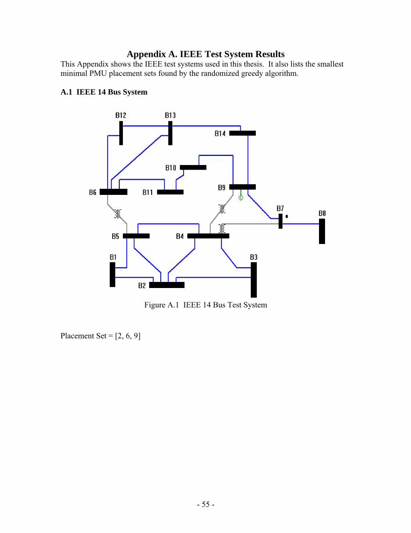
Appendix A. IEEE Test System Results This Appendix shows the IEEE test systems used in this thesis. It also lists the smallest minimal PMU placement sets found by the randomized greedy algorithm. A.1 IEEE 14 Bus System

Figure A.1 IEEE 14 Bus Test System

Placement Set = [2, 6, 9]

- 55 -

A.2 IEEE 57 Bus System

Figure A.2 IEEE 57 Bus Test System

Placement Set = [1, 6, 13, 19, 25, 29, 32, 38, 51, 54, 56]

- 56 -

A.3 IEEE 118 Bus System

Figure A.3 IEEE 118 Bus Test System

Placement Set = [2, 8, 11, 12, 17, 21, 25, 29, 34, 35, 40, 45, 49, 53, 56, 62, 72, 75, 77, 80, 85, 86, 91, 94, 102, 105, 110, 114]

- 57 -

Appendix B. Reduction Program The following MatLab program translates a system model in PSS/E RAW format into the placement model as described in Chapter 4. %This program performs transformer and dummy bus reduction for systems %in PSS/E RAW format rawfilename = input('please enter RAW Format file name --- ', 's'); fid = fopen(rawfilename, 'r'); title = fgetl(fid); baseMVA = str2num(title(32:37)); line = fgets(fid); line = fgets(fid); % ----- get bus data, feed them into matrix bus, gen, gencost, and area ibus = 0; iinject = 0; ibranch = 1; itrans = 0; itrans=0; idel=0; clear deletedbus; area=[]; i=0; x=0; clear branch; clear bus; clear injection; clear trans; while 1>0 i=i+1; line = fgets(fid); if line(1:3)=='0 /' break end ibus = ibus + 1; bus(ibus, 1) = str2num(line(1:6)); % bus number bus(ibus, 2)=0; bus(ibus, 3) = str2num(line(23:31)); busarray(bus(ibus,1),1)=bus(ibus, 1);

- 58 -

busarray(bus(ibus,1),3)=bus(ibus, 3); end i=0; % finds injection buses from list of generators and loads while 1 line = fgets(fid); if line(1:3)=='0 /' break end iinject = iinject + 1; injection(iinject) = str2num(line(1:6)); end while 1 line = fgets(fid); if line(1:3)=='0 /' break end iinject = iinject + 1; injection(iinject) = str2num(line(1:6)); end injection=unique(injection); iinject=size(injection); for i=1:ibus if intersect(bus(i,1), injection)==bus(i,1) bus(i,2)=1; end end branch=[0, 0]; %Creates initial branch list from RAW branch list while 1 line = fgets(fid); if line(1:3)=='0 /' break end a=str2num(line(1:6));

- 59 -

b=abs(str2num(line(8:14))); x=str2num(line(15)); if branch(ibranch, 1)==a && branch(ibranch, 2) ==b else ibranch = ibranch + 1; branch(ibranch, 1) = a; branch(ibranch, 2) = b; end end branch(1,:)=[]; ibranch=length(branch(:,1)); %reads in transformer data while 1 line = fgets(fid); if line(1:3)=='0 /' break end itrans = itrans + 1; trans(itrans,1) = str2num(line(1:6)); trans(itrans,2) = str2num(line(8:13)); trans(itrans,3) = str2num(line(15:20)); line=fgets(fid); line=fgets(fid); line=fgets(fid); end link=eye(ibus); for i=1:ibus xbus=bus(i,1); for x=1:iinject if bus(i,1)==injection(x) bus(i,2)=1; end end end %performs transformer reduction for i=1:itrans clear b1; clear b2; clear b3;

- 60 -

b3=[0 0]; for x=1:ibus if bus(x,1)~=0 if bus(x,1)==trans(i,1) b1=[bus(x,3) x]; end if bus(x,1)==trans(i,2) b2=[bus(x,3) x]; end if bus(x,1)==trans(i,3) b3=[bus(x,3) x]; end end end a=[b1;b2;b3]; a=sortrows(a); %2 winding trans if a(1,1)==0 Rindex=a(3,2); Dindex2=a(2,2); if bus(Rindex,1)~=bus(Dindex2,1) idel=idel+1; deletedbus(idel,1)=bus(Dindex2,1); deletedbus(idel,2)=bus(Rindex,1); [bus, branch, trans,t]=busreplacement(Rindex,Dindex2,bus,branch,trans,itrans); end else %3 winding trans Rindex=a(3,2); Dindex3=[a(1,2) a(2,2)]; if bus(Rindex,1)~=bus(Dindex3(1),1)&& bus(Rindex,1)~=bus(Dindex3(2),1) idel=idel+1; deletedbus(idel,1)=bus(Dindex3(1),1); deletedbus(idel,2)=bus(Rindex,1); idel=idel+1; deletedbus(idel,1)=bus(Dindex3(2),1); deletedbus(idel,2)=bus(Rindex,1); [bus, branch, trans,t]=busreplacement(Rindex,Dindex3,bus,branch,trans,itrans); end end if 0<t&&t<i i=t end trans(i,:); i; end

- 61 -

i=1; while 1 if bus(i,1)==0 bus(i,:)=[]; else i=i+1; if i>=length(bus(:,1)) break end if i==987 g=12; end end if i>=length(bus(:,1)) break end end ibus=length(bus(:,1)); clear injectionindex; clear noinjectndx; ninject=1; iinject=1; for i=1:ibus if bus(i,2)==1 injectionindex(iinject)=i; iinject=iinject+1; else noinjectndx(ninject)=i; ninject=ninject+1; end end for i=1:ibranch for x=1:ibus if branch(i,1)==bus(x,1) bbranch(i,1)=x; end if branch(i,2)==bus(x,1) bbranch(i,2)=x; end end end

- 62 -

%This function updates the bus, branch, and injection lists %when a reduction step happens function [bus, branch, trans, newtrannum]=busreplacement(Rindex,Dindex,bus,branch,trans,itrans) t=0; for i=1:length(Dindex) %replace in branch list for x=1:length(branch) if branch(x,1)==bus(Dindex(i),1) branch(x,1)=bus(Rindex); end if branch(x,2)==bus(Dindex(i),1) branch(x,2)=bus(Rindex); end end for s=1:itrans if trans(s,1)==bus(Dindex(i),1) trans(s,1)=bus(Rindex,1); t=[t s]; end if trans(s,2)==bus(Dindex(i),1) trans(s,2)=bus(Rindex,1); t=[t s]; end if trans(s,3)==bus(Dindex(i),1) trans(s,3)=bus(Rindex,1); t=[t s]; end end if bus(Dindex(i),2)==1 %check if replaced bus inherits injection from deleted bus bus(Rindex,2)=1; end bus(Dindex,1)=0; sort(t) newtrannum=t(1); end

- 63 -