A Performance Estimation Flow for Embedded...
8
A Performance Estimation Flow for Embedded Systems with Mixed Software/Hardware Modeling Joffrey Kriegel Thales Communications University of Nice Sophia-Antipolis France Email:[email protected] Alain Pegatoquet and Michel Auguin University of Nice Sophia-Antipolis Sophia-Antipolis, France Email: [email protected] [email protected] Florian Broekaert Thales Communications Colombes, France Email:fl[email protected] Abstract—This paper introduces an Y-chart methodology for performance estimation based on high level models for both application and architecture. As embedded devices are more and more complex, the choice of the best suited architecture not only in terms of processing power but also in power consumption becomes a tedious task. In this context, estimation tools are key components in architecture choice methodology. Obtained results show an error margin of less than 13% of estimation performance for a H.264 video decoder application on two different hardware platforms. I. I NTRODUCTION Embedded systems processing power, thus complexity, is increasing every day. Current embedded devices for video, im- age, and graphics for instance may include several processors, hardware accelerators or dedicated peripherals in a single chip. With increasing speed and performance capabilities, energy consumption of the system also increases. In the meantime, time-to-market constraints make it essential to quickly react to the needs of the new growing applications. As a consequence, rapid performance estimation tools are becoming more and more necessary for designing or selecting the best target architecture. Selecting a processor for this architecture that fits as much as possible the computing requirements of the targeted applications is required to reduce the chip area, then the cost, but also to reduce the overall power consumption. In this context, Architecture Space Exploration (ASE) techniques help designers to propose more efficient embedded platform implementations [1]. ASE consists in estimating performance and/or power consumption for a large set of hardware config- urations, thus selecting the best efficient solution for potential implementation. In this paper, we propose a performance estimation flow for embedded systems based on a mixed hardware/software modeling. This flow uses both existing [2] and newly devel- oped tools. The application is described using a new UML- like modeling language and is then annotated with dynamic information obtained by profiling. Another contribution of this work is a low level benchmark based approach that allows characterizing hardware parameters in terms of performance constraints. Our solution is evaluated for two versions of the H.264 video decoder application on both OMAP and IMX31 target platforms. We show that estimation results are accurate and could be used for early design space exploration. This paper is organized as follows: Related works is dis- cussed in Section II. Section III discusses impacts of architec- tural choices on performance. In Section IV, results obtained with the QEMU emulator are presented. Section V discusses in detail the application and hardware models used in our methodology. Finally experimental results and conclusions are discussed in Section VI and VII. II. RELATED WORKS Having a precise model of the software application is key in performance estimation. In order to get pertinent information of an application, profiling techniques are commonly used. Gprof, the GNU profiler uses information collected during the actual execution of the program. Thus, Gprof provides dynamic information that represents the number of executions of each statements (or basic block) as well as the time spent by each function. Although this kind of metrics is useful, additional information such as the number of memory accesses or the number of executed instructions is needed for accurate estimation. Valgrind [2] instrumentation framework provides such metrics. It is a powerful set of tools to profile a multi- threaded application written in many programming languages. • Callgrind is used to get the number of threads, the func- tions dependencies and the number of host instructions executed by each function. • Cachegrind outputs the number of read and write memory accesses of each functions as well as the number of cache miss. Cachegrind provides percentage as well. All these tools provide information collected during the execution of the program. As a consequence, provided infor- mation are rather based on an average execution time than a worst-case execution time (WCET). In [3], authors describe different approaches to determine the WCET and survey sev- eral commercially available tools and research prototypes. Al- though the problem of determining upper bounds on execution times for single tasks and for quite complex processor architec- tures has been solved, available tools remain inappropriate for instance for complex applications with deeply interdependent or nested control structures. Moreover, determining the WCET is a hard problem if the underlying processor architecture has components such as caches, pipelines, branch prediction and 978-1-4577-0801-5/11/$26.00 ©2011 IEEE 174
Transcript of A Performance Estimation Flow for Embedded...

A Performance Estimation Flow for Embedded
Systems with Mixed Software/Hardware Modeling
Joffrey Kriegel
Thales Communications
University of Nice Sophia-Antipolis
France
Email:[email protected]
Alain Pegatoquet and Michel Auguin
University of Nice Sophia-Antipolis
Sophia-Antipolis, France
Email: [email protected]
Florian Broekaert
Thales Communications
Colombes, France
Email:[email protected]
Abstract—This paper introduces an Y-chart methodology forperformance estimation based on high level models for bothapplication and architecture. As embedded devices are more andmore complex, the choice of the best suited architecture not onlyin terms of processing power but also in power consumption
becomes a tedious task. In this context, estimation tools are keycomponents in architecture choice methodology. Obtained resultsshow an error margin of less than 13% of estimation performancefor a H.264 video decoder application on two different hardwareplatforms.
I. INTRODUCTION
Embedded systems processing power, thus complexity, is
increasing every day. Current embedded devices for video, im-
age, and graphics for instance may include several processors,
hardware accelerators or dedicated peripherals in a single chip.
With increasing speed and performance capabilities, energy
consumption of the system also increases. In the meantime,
time-to-market constraints make it essential to quickly react to
the needs of the new growing applications. As a consequence,
rapid performance estimation tools are becoming more and
more necessary for designing or selecting the best target
architecture. Selecting a processor for this architecture that
fits as much as possible the computing requirements of the
targeted applications is required to reduce the chip area, then
the cost, but also to reduce the overall power consumption. In
this context, Architecture Space Exploration (ASE) techniques
help designers to propose more efficient embedded platform
implementations [1]. ASE consists in estimating performance
and/or power consumption for a large set of hardware config-
urations, thus selecting the best efficient solution for potential
implementation.
In this paper, we propose a performance estimation flow
for embedded systems based on a mixed hardware/software
modeling. This flow uses both existing [2] and newly devel-
oped tools. The application is described using a new UML-
like modeling language and is then annotated with dynamic
information obtained by profiling. Another contribution of this
work is a low level benchmark based approach that allows
characterizing hardware parameters in terms of performance
constraints. Our solution is evaluated for two versions of the
H.264 video decoder application on both OMAP and IMX31
target platforms. We show that estimation results are accurate
and could be used for early design space exploration.
This paper is organized as follows: Related works is dis-
cussed in Section II. Section III discusses impacts of architec-
tural choices on performance. In Section IV, results obtained
with the QEMU emulator are presented. Section V discusses
in detail the application and hardware models used in our
methodology. Finally experimental results and conclusions are
discussed in Section VI and VII.
II. RELATED WORKS
Having a precise model of the software application is key in
performance estimation. In order to get pertinent information
of an application, profiling techniques are commonly used.
Gprof, the GNU profiler uses information collected during
the actual execution of the program. Thus, Gprof provides
dynamic information that represents the number of executions
of each statements (or basic block) as well as the time spent
by each function. Although this kind of metrics is useful,
additional information such as the number of memory accesses
or the number of executed instructions is needed for accurate
estimation. Valgrind [2] instrumentation framework provides
such metrics. It is a powerful set of tools to profile a multi-
threaded application written in many programming languages.
• Callgrind is used to get the number of threads, the func-
tions dependencies and the number of host instructions
executed by each function.
• Cachegrind outputs the number of read and write memory
accesses of each functions as well as the number of cache
miss. Cachegrind provides percentage as well.
All these tools provide information collected during the
execution of the program. As a consequence, provided infor-
mation are rather based on an average execution time than a
worst-case execution time (WCET). In [3], authors describe
different approaches to determine the WCET and survey sev-
eral commercially available tools and research prototypes. Al-
though the problem of determining upper bounds on execution
times for single tasks and for quite complex processor architec-
tures has been solved, available tools remain inappropriate for
instance for complex applications with deeply interdependent
or nested control structures. Moreover, determining the WCET
is a hard problem if the underlying processor architecture has
components such as caches, pipelines, branch prediction and
978-1-4577-0801-5/11/$26.00 ©2011 IEEE 174

other speculative components, which is definitively the kind
of architecture that we use. Finally, several features such as
pointers to data or to functions, or dynamically allocated data
can easily ruin precision of WCET estimation tools.
Having a precise model of the target platform is also key
in performance estimation. A common solution to model a
platform is to use an ISS (Instruction Set Simulator) and to
describe the remaining parts of the platform (memories and
peripherals) using a modeling language such as VHDL or
SystemC. With the emergence of transaction level modeling
(TLM) approaches, different companies have recently offered
virtual prototyping environment. The advantage of TLM is
to drastically reduce simulation time compared to RTL level
based simulation. With an execution speed of several 10s
of million instructions per second, a TLM-based platform is
capable of running OSs such as Linux in a matter of seconds.
Another advantage of such a technology is that the real code
of the application can be executed on the virtual platform,
and so software can be validated early in the design phase (at
pre-silicon stage). As example, Innovator [4], Coware [5] or
Simics [6] tools are platform driven ESL (Electronic System
Level) design solutions respectively available from Synopsys
and Virtutech. In [7], authors propose a methodology for
exploration based on an architecture simulation tool (Sim-
pleScalar [8]) to get the performance of each function of the
test application. The main drawback of such kind of tool is that
each application has to be executed on each processor before
doing exploration. Moreover, SimpleScalar does not emulate
brand new processors such as the ARM Cortex-A9.
Another recent offer is QEMU [9] [10], a platform simulator
which contains a lot of different processor models (X86,
ARM, MIPS, SPARC...). QEMU is based on the dynamic
translation of the code. The problem is that this simulator
is not timed. Some extensions using timed-TLM [11] have
been proposed in order to add timing information in QEMU.
However, QEMU itself remains untimed and only the TLM
part is timed. Moreover, the TLM hardware models have
to be developed with high precision in order to take into
account these timing information. Although these solutions
are accurate, modeling a platform is time consuming and
an ISS is required for each processor. As both architecture
and application become more and more complex, another
approach must be considered for rapid performance and power
estimation, thus architecture exploration. In order to decrease
the modeling time, a higher level of abstraction is needed using
for instance UML, SysML [12] or AADL [13]. The advantage
of these languages is that they can model both the software
and the hardware due to their high level of abstraction.
III. TUNING PERFORMANCE WITH DIFFERENT
ARCHITECTURE PARAMETERS
The application used in our experiments is a H.264 decoder
implemented on the ARM Cortex-A8 processor of the Texas
Instruments OMAP3530 EVM platform [14]. The H.264 ap-
plication, written in C language, decodes a video compressed
file in a CIF format (352 x 288) and then writes its result on
a frame buffer. Each video frame is divided into two slices
(image section that can be computed independently) and can
be either an intra or inter prediction type of frame (an intra
frame is more complex to decode than an inter frame). The
application is composed of three independent threads: one
thread is used for the main task while two threads are used to
decode both slices of the video.
The Texas Instruments OMAP3530 hardware platform con-
tains two main processors: a GPP, the ARM Cortex-A8, and a
DSP, the VLIW TMS320C64x+ DSP Core with 8 independent
functional units. So far, only the GPP has been used in our
experiments. This processor has a 32K-Byte L1 cache, a 256K-
Byte L2 cache and up to 512K-Byte external DDR2 Ram. This
platform has been chosen because many hardware parameters
can be customized. For example, the L1 and/or the L2 caches
can be enabled or disabled, the CPU frequency can be adjusted
(from 50 to 800 MHz) as well as the interconnection bus
frequency (at either 83 or 166 MHz), etc.
Fig. 1: H264 video decoder running on the Cortex-A8 with
different hardware parameters.
The Figure 1 displays results obtained for different archi-
tectural configurations of the OMAP3 platform. In order to
measure the performance of the different configurations, as
much frames as possible are decoded for each configuration,
i.e. the frame rate for the input video is not fixed. First,
we can see that when the L2 cache is enabled the overall
performance remains roughly the same (only 0.5% to 6%
decrease) whatever the choice of the L3 bus frequency. In
the other hand, if the L3 bus frequency is set to 166 MHz,
the number of decoded FPS will be highly different if the L2
cache is disabled or enabled. Performance is indeed decreased
by 14% to 39% when the L2 cache is disabled (compared to
a solution with L2 cache enabled). Finally, we can see that
the L3 frequency is an important parameter for the number of
decoded FPS when the L2 cache is disabled. As shown on the
Figure 1, in that case a decrease of performance from 3.5% to
28% can be observed. In conclusion, these experiments clearly
demonstrate that performance (here in terms of number of
decoded FPS) of the H.264 video decoding application highly
175
depends on these parameters. Moreover, all these architectural
parameters are inter-dependent.
The H.264 video decoder source code study has shown
that a lot of computations are required to decode images
(about 74 millions instructions per frame) as well as a lot of
memory accesses to load and store images and to print image
on the output frame buffer (about 39 millions of load/store).
Thus, adjusting the CPU frequency and finding the right
tuning for caches and bus frequency while respecting real-time
constraints is not an easy task for this kind of application. The
H.264 video decoder is then a good use case as performance
is greatly dependent to the architectural choices.
Based on our experiments, we defined several parameters
having a major influence on the overall performance:
• CPU frequency
• L1 cache (avaibility, size, bytes per line...)
• L2 cache (avaibility, size, bytes per line...)
• L3 interconnect bus frequency and width
• Interrupt latency (for real-time applications)
It appears that a global approach is needed in order to
rapidly get pertinent estimations, explore different architec-
tures and then decide which one is the best suited in term of
performance and power consumption (so far only performance
is considered in this paper). The Table I presents three differ-
ent configurations that respect a 10 FPS quality of service
(QoS). Each configuration corresponds to different architec-
tural choices. So, our objective is to define a method that
will help system engineers to find these different architectural
solutions with respect of the timing requirements (or QoS). We
also expect to provide an environment that will help deciding
which configuration is the best in terms of both performance
and power consumption (e.g. the first configuration of Table I
in our case).
Configuration CPU L2 Interconnect Power
name Frequency cache Frequency consumption
Config1 300 MHz Enabled 166 or 83 MHz 954 mJ
Config2 450 MHz Disabled 166 MHz 1012 mJ
Config3 700 MHz Disabled 83 MHz 1439 mJ
TABLE I: Different possible configurations for 10 FPS QoS.
In case the real platform is not available (at pre-silicon phase
for instance), a solution consists in evaluating the performance
of an hardware platform using a virtual platform such as
QEMU [9].
IV. RESULTS WITH QEMU VS REAL-PLATFORM
QEMU [10] is a generic and open source machine emulator
and virtualizer. When used as a machine emulator, QEMU can
run OSes and programs made for one machine (e.g. an ARM
board) on a different machine (e.g. a PC). By using dynamic
translation, very good performance in terms of simulation
speed can be achieved (a Linux OS can boot on an ARM
device in less than 5 sec.). It is worth noticing that we have
used an extended version of QEMU for our tests (compared
to the version available from [9]). These extensions have
been implemented by the TIMA laboratory [15] in order to
add hardware timing information. Notice that the simulation
platform is still at a development state, so the accuracy can
be further improved.
QEMU contains many processor models and is useful for
modeling a hardware platform. In our case, the hardware
modeled is the CPU (QEMU), the L1 cache and the external
DDR memory (TIMA extensions in SystemC). The CPU is
an ARM Cortex-A8 running at 600MHz with a L1 cache
of 16KB, 4-way associative and lines of 64 bytes. Many
adjustments and tests have been performed on this platform to
tune it with as much accuracy as possible with real hardware
platform. As an example, the cache latency and the number
of cycle(s) per instruction have been particularly investigated
for that purpose. In order to compare performance estimations
provided by QEMU with actual execution time, the H.264
video decoder as well as different benchmarks have been
executed on both the simulation platform and the real platform.
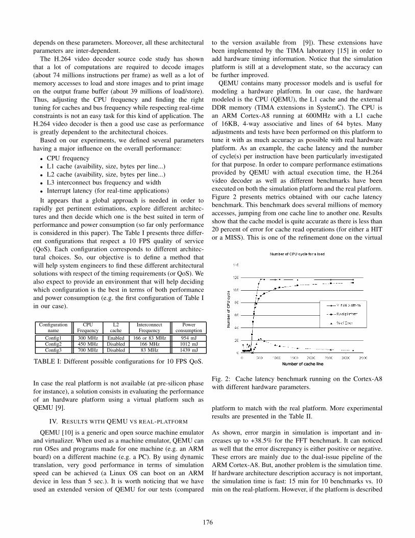
Figure 2 presents metrics obtained with our cache latency
benchmark. This benchmark does several millions of memory
accesses, jumping from one cache line to another one. Results
show that the cache model is quite accurate as there is less than
20 percent of error for cache read operations (for either a HIT
or a MISS). This is one of the refinement done on the virtual
Fig. 2: Cache latency benchmark running on the Cortex-A8
with different hardware parameters.
platform to match with the real platform. More experimental
results are presented in the Table II.
As shown, error margin in simulation is important and in-
creases up to +38.5% for the FFT benchmark. It can noticed
as well that the error discrepancy is either positive or negative.
These errors are mainly due to the dual-issue pipeline of the
ARM Cortex-A8. But, another problem is the simulation time.
If hardware architecture description accuracy is not important,
the simulation time is fast: 15 min for 10 benchmarks vs. 10
min on the real-platform. However, if the platform is described
176

Test Real platform simulated platform errorname (iteration / sec) (iteration / sec) ( % )
Numeric Sort 147.04 97.68 -33.5
Bitfield 3.14 2.87 -8.8
Fourier 577 799 +38.5
Assignement 0.877 0.999 +13.9
IDEA Encryption 482.3 442.3 -8.3
Huffman 187.6 193.8 +3.3
( FPS ) ( FPS ) ( % )
H.264 decoder 13.9 9.1 -34.5
TABLE II: Comparison between simulation and real-platform.
with more details (L1 cache, communication bus, custom IP,
...) the simulation time significantly increases: up to 1 day
for the 10 benchmarks if the interconnect bus is modeled for
instance. As a consequence, adding more architectural details
in QEMU currently leads to an unsatisfying situation: simu-
lation time is impracticable for exploration while estimation
results are not necessarily better... Although QEMU is a good
solution for application code and drivers validation, a simpler
and clever tool is required to quickly explore architectures
and find the more appropriate hardware architecture for the
targeted performance.
V. BENCHMARK BASED APPROACH
In this section, a methodology based on high level modeling
tools for both hardware and software is proposed for quickly
evaluating the performance level of an application running on
a hardware platform.
Fig. 3: Global estimation tool flow.
Figure 3 above depicts this estimation tool flow. As output,
this tool is able to generate a hardware-constrained model
of the application that can be executed on a host computer.
As shown on the Figure 3, our methodology is based on
the Y-chart design principle. Similar approaches have been
proposed in the past such as SESAME [16], Metroplis [17] or
Milan [18]. For example, in SESAME the functional behavior
of an application is described in an architecture independent
manner. Then a platform architecture model defines archi-
tecture resources and captures their performance constraints.
Finally, an explicit mapping step maps an application model
onto an architecture model for co-simulation, after which
the system performance can be evaluated quantitatively. The
main drawback of this kind of environment is that they make
use of an ISS/RTL simulator of the target processor for
calibrating the latencies of the programmable components in
the architecture model (DSP, ASIP and so on). Our approach is
ISS-independent and rather based on a high level model of the
application annotated with dynamic information. For that, the
application is profiled on the host machine. Low level bench-
marks or datasheets are used to characterize the hardware
platform. Then, both application and hardware models are
mapped into a hardware-constrained model of the application.
A. Application model
The target application software architecture is described
using a custom language based on a UML-like type of model-
ing: functional blocks and connections between them are de-
scribed. Connections can be either synchronous, asynchronous
or deferred synchronous. A block can be composed of several
tasks, each task being one or several threads. Dependencies
and priorities (i.e. preemptions) can be defined at either task
or thread level. A block is activated as soon as an incoming
signal onto one of these input ports is arrived. Then a signal
is generated onto one of this output after a certain amount
of time or number of operations. An executable C++ code
can be generated from this specification using configuration
text files. A configuration file is required for each block
and also for the architecture top level description (describing
interactions between blocks). Configurations files are split into
three distinct parts:
• Component: describes the external view of the block
through input and output signals definition. As an exam-
ple, Listing 1 shows a definition for the main component
(main comp) of the H.264 application. Provides and uses
keywords respectively define input and output signals for
that component.
• Behavior: defines the behavior of the block when an input
signal is received. For that purpose, a state number (if
a state machine is defined), the output signal and its
corresponding number of activation must be specified.
As an example, Listing 2 describes the behavior defini-
tion (main behavior) of the main component previously
defined (main comp). This definition indicates that each
time the input timer signal is received, the comm slice1
and the comm slice2 output signals will be generated.
For this block behavioral description, no state machine is
required. This is expressed by the (1) statement which
means that only one state is possible. The following
parameters (equal to 1 for both output signals) indicate
the number of times output signals will be generated. This
feature allows defining multi-rate system.
• Characteristics: defines the CPU processing time or the
number of operations to execute when a input signal is
received. For instance, Listing 3 depicts the processing
time characteristics that corresponds to the behavior of
the component. This is achieved by indicating “Tim-
ing in ms” after the characteristics keyword. This listing
shows the way timing can be defined onto input signal
177

reception and before output signal activation. The (1)
statement means that only one state is possible. Then
0.05 indicates the execution time in ms required by the
input timer component before comm slice1 output signal
is activated. Finally, the last parameter which is equal to
0 indicates that there is no processing time after output
signals activation.
component main comp{
p r o v i d e s Runnable i n p u t t i m e r ;
u s e s Runnable comm slice1 ;
u s e s Runnable comm slice2 ;p r o v i d e s Runnable i n p u t s l i c e 1 ;
p r o v i d e s Runnable i n p u t s l i c e 2 ;
u s e s Runnable comm wri te buf fe r ;} ;
Listing 1: An example illustrating the Component definition
for the H.264 application.
b e h a v i o u r main behav iour of main comp{
i n p u t t i m e r . run
{( 1 ) 1 { comm slice1 . run } 1 { comm slice2 . run }
}. . .
}
Listing 2: An example illustrating part of the Behaviour
definition for the maincomp component.
c h a r a c t e r i s t i c s ( Timing in ms ) m a i n t i m i n g c h a r a c s
of main behav iour{
i n p u t t i m e r . run
{( 1 ) { 0 . 0 5 0 0 }
}. . .
}
Listing 3: An example illustrating the Characteristics definition
of the inputtimer of the maincomp component.
Architecture files define the way blocks are connected. After
having included blocks configuration files, blocks must be
instantiated in order to declare a behavior and characteristics
for each block. Then, connections between blocks must be
specified through input/output signals. The Listing 4 depicts
the top level architecture file for the H.264 application. As
shown, all required blocks are instanciated using the “compo-
nent instance” keyword. As an example, “main” is an instance
of the “main behaviour” with reference to its CPU processing
time “main timing characs” previously defined.
Actually, the listing 4 is used to automatically generate the
graphical representation of the H.264 application presented on
i n c l u d e main . t x t ;
c o m p o n e n t i n s t a n c e main behav iour main
m a i n t i m i n g c h a r a c s ;
c o m p o n e n t i n s t a n c e s l i c e b e h a v i o u r s l i c e 1s l i c e t i m i n g c h a r a c s ;
c o m p o n e n t i n s t a n c e s l i c e b e h a v i o u r s l i c e 2
s l i c e t i m i n g c h a r a c s ;
c o m p o n e n t i n s t a n c e Timer impl t 1 t i m e r ;. . .
Listing 4: An example illustrating the system software
architecture definition for a H.264 application.
Figure 4. The C++ code generated from this specification can
be executed on any platform respecting the POSIX standard,
in order to verify for instance the right scheduling of tasks or
that real-time constraints are respected. For that the application
model has to be annotated with dynamic information such as
the number of instructions to execute, the number of memory
load/store and the size of memory print. Next section describes
how the dynamic information are collected from an existing
application.
B. Dynamic information
Collecting dynamic information is done through profiling
the application. For that, the software application is executed
on the host machine (a PC in our case) with the Valgrind tools
set to collect execution information. Callgrind and Cachegrind
are tools available from the Valgrind environment. The fol-
lowing application related parameters are determined using
Callgrind:
• nb insn: number of Dhrystone assembly instructions per
thread.
• nb r: number of memory read access (load) per iteration.
• nb w: number of memory writes access (store) per iter-
ation.
The following application related parameters are determined
using Cachegrind:
• l1 miss rate: percentage of L1 cache misses for the target
application.
• l2 miss rate: percentage of L2 cache misses for the target
application.
Note that the user has to provide the size and the type of the
cache, as well as the number of bytes per line to Cachegrind
tool. In order to get an averaged value for these parameters,
the target application is executed for a number of iterations
(e.g. 50 iterations (or images) for the H.264 video decoder).
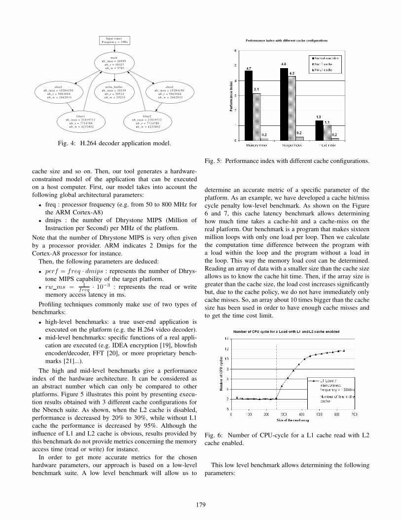
Figure 4 shows the corresponding graphical model of the
H.264 decoder annotated with dynamic information. The ap-
plication model is then processed by a script with collected
information presented above.
C. Hardware architecture model
A model of the target architecture also has to be provided
in our framework. Our model describes the main architec-
tural characteristic parameters like the CPU frequency, the
178
main
nb_ insn = 20599
nb_r = 10327
n b _ w = 5 7 8 3
slice1
nb_ insn = 15284150
nb_ r = 5063044
n b _ w = 2 4 6 2 9 3 3
slice2
nb_ insn = 15284150
nb_ r = 5063044
n b _ w = 2 4 6 2 9 3 3
write_buffer
nb_ insn = 10239
nb_r = 30512
n b _ w = 2 5 2 3 3
filter1
nb_ insn = 21819712
nb_ r = 7714788
n b _ w = 4 2 3 3 8 0 2
filter2
nb_ insn = 21819712
nb_ r = 7714788
n b _ w = 4 2 3 3 8 0 2
Input t imer
Frequency = 15Hz
Fig. 4: H.264 decoder application model.
cache size and so on. Then, our tool generates a hardware-
constrained model of the application that can be executed
on a host computer. First, our model takes into account the
following global architectural parameters:
• freq : processor frequency (e.g. from 50 to 800 MHz for
the ARM Cortex-A8)
• dmips : the number of Dhrystone MIPS (Million of
Instruction per Second) per MHz of the platform.
Note that the number of Dhrystone MIPS is very often given
by a processor provider. ARM indicates 2 Dmips for the
Cortex-A8 processor for instance.
Then, the following parameters are deduced:
• perf = freq · dmips : represents the number of Dhrys-
tone MIPS capability of the target platform.
• rw ms = 1
freq· 10−3 : represents the read or write
memory access latency in ms.
Profiling techniques commonly make use of two types of
benchmarks:
• high-level benchmarks: a true user-end application is
executed on the platform (e.g. the H.264 video decoder).
• mid-level benchmarks: specific functions of a real appli-
cation are executed (e.g. IDEA encryption [19], blowfish
encoder/decoder, FFT [20], or more proprietary bench-
marks [21]...).
The high and mid-level benchmarks give a performance
index of the hardware architecture. It can be considered as
an abstract number which can only be compared to other
platforms. Figure 5 illustrates this point by presenting execu-
tion results obtained with 3 different cache configurations for
the Nbench suite. As shown, when the L2 cache is disabled,
performance is decreased by 20% to 30%, while without L1
cache the performance is decreased by 95%. Although the
influence of L1 and L2 cache is obvious, results provided by
this benchmark do not provide metrics concerning the memory
access time (read or write) for instance.
In order to get more accurate metrics for the chosen
hardware parameters, our approach is based on a low-level
benchmark suite. A low level benchmark will allow us to
Fig. 5: Performance index with different cache configurations.
determine an accurate metric of a specific parameter of the
platform. As an example, we have developed a cache hit/miss
cycle penalty low-level benchmark. As shown on the Figure
6 and 7, this cache latency benchmark allows determining
how much time takes a cache-hit and a cache-miss on the
real platform. Our benchmark is a program that makes sixteen
million loops with only one load per loop. Then we calculate
the computation time difference between the program with
a load within the loop and the program without a load in
the loop. This way the memory load cost can be determined.
Reading an array of data with a smaller size than the cache size
allows us to know the cache hit time. Then, if the array size is
greater than the cache size, the load cost increases significantly
but, due to the cache policy, we do not have immediately only
cache misses. So, an array about 10 times bigger than the cache
size has been used in order to have enough cache misses and
to get the time cost limit.
Fig. 6: Number of CPU-cycle for a L1 cache read with L2
cache enabled.
This low level benchmark allows determining the following
parameters:
179
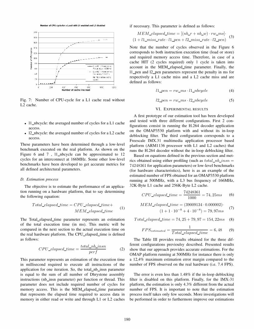
Fig. 7: Number of CPU-cycle for a L1 cache read without
L2 cache.
• l1 nbcycle: the averaged number of cycles for a L1 cache
access.
• l2 nbcycle: the averaged number of cycles for a L2 cache
access.
These parameters have been determined through a low-level
benchmark executed on the real platform. As shown on the
Figure 6 and 7 , l1 nbcycle can be approximated to 12
cycles for an interconnect at 166MHz. Some other low-level
benchmarks have been developed to get accurate metrics for
all defined architectural parameters.
D. Estimation process
The objective is to estimate the performance of an applica-
tion running on a hardware platform, that to say determining
the following equation:
Total elapsed time = CPU elapsed time+
MEM elapsed time(1)
The Total elapsed time parameter represents an estimation
of the total execution time (in ms). This metric will be
compared in the next section to the actual execution time on
the real hardware platform. The CPU elapsed time is defined
as follows:
CPU elapsed time =total nb insn
perf(2)
This parameter represents an estimation of the execution time
in millisecond required to execute all instructions of the
application for one iteration. So, the total nb insn parameter
is equal to the sum of all number of Dhrystone assembly
instructions (nb insn parameter) per function or thread. This
parameter does not include required number of cycles for
memory access. This is the MEM elapsed time parameter
that represents the elapsed time required to access data in
memory in either read or write and through L1 or L2 caches
if necessary. This parameter is defined as follows:
MEM elapsed time = [(nb r + nb w) · rw ms]·
(1 + l1 miss rate · l1 pen + l2 miss rate · l2 pen)(3)
Note that the number of cycles observed in the Figure 6
corresponds to both instruction execution time (load or store)
and required memory access time. Therefore, in case of a
cache HIT (2 cycles required) only 1 cycle is taken into
account in the MEM elapsed time parameter. Finally, the
l1 pen and l2 pen parameters represent the penalty in ms for
respectively a L1 cache miss and a L2 cache miss and are
defined as follows:
l1 pen = rw ms · l1 nbcycle (4)
l2 pen = rw ms · l2 nbcycle (5)
VI. EXPERIMENTAL RESULTS
A first prototype of our estimation tool has been developed
and tested with three different configurations. First 2 con-
figurations consist in running the H.264 decoder application
on the OMAP3530 platform with and without its in-loop
deblocking filter. The third configuration corresponds to a
Freescale IMX.31 multimedia application processor based
platform (ARM1136 processor with L1 and L2 caches) that
runs the H.264 decoder without the in-loop deblocking filter.
Based on equations defined in the previous section and met-
rics obtained using either profiling (such as total nb insn =74248361 for application parameters) or low-level benchmarks
(for hardware characteristics), here is as an example of the
estimated number of FPS obtained for an OMAP3530 platform
running at 500MHz, with a L3 bus frequency of 166MHz,
32K-Byte L1 cache and 256K-Byte L2 cache.
CPU elapsed time =74248361
1000= 74, 25ms (6)
MEM elapsed time = (39009134 · 0.000002)·
(1 + 1 · 10−8 + 4 · 10−8) = 79, 97ms(7)
Total elapsed time = 74, 25 + 79, 97 = 154, 22ms (8)
FPSestimated =1
Total elapsed time= 6, 48 (9)
The Table III provides results obtained for the three dif-
ferent configurations previoulsy described. Presented results
show that our approach provides accurate estimations. For the
OMAP platform running at 500MHz for instance there is only
a 12,4% maximum estimation error margin compared to the
number of FPS observed on the real hardware (i.e. 7.4 FPS).
The error is even less than 1.48% if the in-loop deblocking
filter is disabled on this platform. Finally, for the IMX-31
platform, the estimation is only 4.3% different from the actual
number of FPS. It is important to note that the estimation
process itself takes only few seconds. More investigations will
be performed in order to furthermore improve our estimations
180

Platform name Real platform custom tool error
With filter ( FPS ) ( FPS ) ( % )OMAP3 @ 600MHz 8.9 7.8 12.5
OMAP3 @ 500MHz 7.4 6.5 12.4
OMAP3 @ 250MHz 3.7 3.2 12.4
OMAP3 @ 125MHz 1.8 1.6 10
IMX.31 @ 532MHz 5.5 5.35 2.7
Without filter ( FPS ) ( FPS ) ( % )
OMAP3 @ 600MHz 19.3 19.16 0.7
OMAP3 @ 500MHz 16.1 15.96 0.9
OMAP3 @ 250MHz 8.1 7.98 1.5
OMAP3 @ 125MHz 4 3.99 0.25
IMX.31 @ 532MHz 12.6 13.1 4.3
Max. error 12.5
Mean error 5.8
TABLE III: Comparison between custom-tool estimation and
real-platform.
accuracy. For instance, the H.264 video decoder with its in-
loop deblocking filter still provides estimations errors that need
to be improved.
Platform name x86 ARM difference ( % )
With filter
total nb insn 3712418033 3302398898 11
nb w 1279783228 958862304 25
nb r 670673474 526536751 21.5
Without filter ( % )
total nb insn 1529944972 1524018057 0.4
nb w 508337779 381628784 25
nb r 247282385 208018352 15.9
TABLE IV: Host (x86) vs. target (ARM) platform estimation
errors.
These discrepancies are mainly due to estimation errors for
both the number of instructions and memory accesses. As
shown on the Table IV, the number of read/write memory
accesses between x86 and ARM processor is up to 25.08%
different while the number of instructions differs from 0.39 to
11.04%. Hopefully, for the H.264 application there is much
more instructions than memory accesses, so that the final
performance estimation depends mainly on the right estimation
of the number of instructions (which is acceptable). As a
conclusion we consider that an error margin of about 10%
on the final estimation is acceptable since our tool is intended
to be used early in the design flow. However, our future works
will be focused on improving estimations for the memory
accesses as well as the number of instructions.
VII. CONCLUSION
In this paper we have presented different existing ap-
proaches to evaluate the performance of a hardware platform.
Corresponding environments or tools are generally too long to
develop or not appropriate for rapid estimation. We proposed
a new methodology to get a quick performance estimation of
a defined architecture. This tool makes use of a basic model of
the application annotated with dynamic information collected
during execution and a model of the hardware architecture
based on performance parameters using specific low level
benchmarks. Results obtained so far show that estimations are
very accurate for two different platforms with two software
configurations. Future works will be focused on generic mod-
els for hardware characteristics. As an example we plan to use
a generic cache model. Then estimations for a multiprocessor
platform will also need to be addressed. Finally, we intend to
extend our hardware models used for architecture exploration
with power consumption information.
REFERENCES
[1] M. GRIES - “Methods for Evaluating and Covering the Design Space
during Early Design Development”, Integration, the VLSI Journal, Else-
vier, Vol. 38, Issue 2, pages 131-183, 2004.[2] VALGRIND : http://valgrind.org
[3] R. WILHELM et al. - “The Worst-Case Execution Time Problem -
Overview of Methods and Survey of Tools”, ACM Transactions on
Embedded Computing Systems (TECS), Volume 7 Issue 3, April 2008.[4] A. PEGATOQUET, F. Thoen, D. Paterson - “Virtual Reality for 2.5G
Wireless Communication Modem Software Development”, 32nd Annual
IEEE International Computer Software and Applications Conference(COMPSAC), Turku, Finland, July 28-August 1, 2008.
[5] D. VERKEST, K. Van Rompaey, I. Bolsens and H. De Man - “CoWare,
a design environment for heterogeneous hardware/software systems”,
Readings in hardware/software co-design, Kluwer Academic PublishersNorwell, pp. 412-426, 2002.
[6] P. S. MAGNUSSON et al. - Simics : A full system simulation platform,
Computer, vol. 35, no. 2, pp. 50-58, Feb. 2002.[7] A. SIMALATSAR, R. Passerone, D. Densmore - A methodology for
architecture exploration and performance analysis using system level
design languages and rapid architecture profiling, IEEE International
Symposium on Industrial Embedded Systems (SIES), 2008.[8] D. BURGER and T. M. Austin - The simplescalar tool set, version 2.0,
SIGARCH Comput. Archit. News, vol. 25, no. 3, pp. 13-25, 1997.
[9] QEMU : http://wiki.qemu.org.[10] F. BELLARD - QEMU, a Fast and Portable Dynamic Translator,
FREENIX Track: USENIX Annual Technical Conference, 2005.
[11] M. BECKER, G. Di Guglielmo, F. Fummi, W. Mueller, G. Pravadelli,
T. Xie - RTOS-Aware Refinement for TLM2.0-based HW/SW Designs,Design, Automation & Test in Europe Conference & Exhibition, 2010.
[12] Y. VANDERPERREN and W. Dehane - ”SysML and Systems Engineering
Applied to UML-Based SoC Design”, Proceedings of the 2nd UML-SoC
Workshop at 42nd DAC, Anaheim (CA), USA, 2005.[13] 0. SOKOLSKY, I. Lee and D. Clarke - Schedulability analysis of AADL
models, 20th International Parallel and Distributed Processing Symposium
(IPDPS), Rhodes Island, Greece, 25-29 April 2006.[14] OMAP3530 Application processor, Texas Instruments. Dallas, Texas.
http://focus.ti.com/docs/prod/folders/ print/omap3530.html
[15] RABBIT PROJECT OF TIMA - http://tima-
sls.imag.fr/www/research/rabbits[16] C. ERBAS, A.D. Pimentel, M. Thompson, and S. Polstra - A Framework
for System-Level Modeling and Simulation of Embedded Systems Archi-
tectures, EURASIP Journal on Embedded Systems, Volume 2007 Issue1, January 2007.
[17] F. BALARIN, Y. Watanabe, H. Hsieh, L. Lavagno, C. Passerone and
A. Sangiovanni-Vincentelli - Metropolis: an integrated electronic system
design environment, Computer, vol. 36, no. 4, pp. 4552, 2003.[18] S. MOHANTY and V. K. Prasanna - Rapid system-level performance
evaluation and optimization for application mapping onto SoC architec-
tures, in Proceedings of the 15th Annual IEEE International ASIC/SOCConference, pp. 160167, Rochester, NY, USA, September 2002.
[19] S. CHO and Y. Kim - “Linux BYTEmark Benchmarks: A Performance
Comparison of Embedded Mobile Processors”, IEEE The 9th Interna-
tional Conference on Advanced Communication Technology, Feb. 2007[20] M. R. GUTHAUS, J. S. Pingenberg, D. Emst, T. M. Austin, T. Mudge,
R. B. Brown - “MiBench: A free, commercially representative embedded
benchmark suite”, WWC-4. IEEE International Workshop on Workload
Characterization, 2001[21] EEMBC - http://www.eembc.org/home.php
181


![Memory-architecture aware compilation · Optimizations, Workshop on Embedded Computer Systems: Architectures, Modeling, and Simulation (SAMOS VI), 2006]. Application C code Memory](https://static.fdocuments.net/doc/165x107/603f97702d55f9752278c6d6/memory-architecture-aware-optimizations-workshop-on-embedded-computer-systems.jpg)