Plant Growth and LAI Estimation using quantizedEmbedded Regression models for high throughputphenotypingDhruv Sheth  ( dhruvsheth.linkit@gmail.com )

Ambassador, EdgeImpulse Inc. San Jose, California https://orcid.org/0000-0001-7485-1455

Research Article

Keywords: Precision Agriculture, Embedded Machine Learning, Embedded Systems, Image Regression

Posted Date: November 9th, 2021

DOI: https://doi.org/10.21203/rs.3.rs-1060088/v1

License: This work is licensed under a Creative Commons Attribution 4.0 International License.  Read Full License

1

Plant Growth and LAI Estimation using quantized

Embedded Regression models for high throughput

phenotyping

1st Dhruv. M. Sheth Udayachal High School, Senior Secondary

Embedded Machine Learning Ambassador - EdgeImpulse Inc. San Jose. California

Mumbai, India

dhruvsheth.linkit@gmail.com

Abstract—Phenotyping involves the quantitative assessmentof the anatomical, biochemical, and physiological plant traits.Natural plant growth cycles can be extremely slow, hinderingthe experimental processes of phenotyping. Deep learning offersa great deal of support for automating and addressing keyplant phenotyping research issues. Machine learning-based high-throughput phenotyping is a potential solution to the phenotypingbottleneck, promising to accelerate the experimental cycles withinphenomic research. The influence of climate change, and due toit’s unpredictable nature, majority of agricultural crops havebeen affected in terms of production and maintenance. Hybridand cost-effective crops are making their way into the market,but monitoring factors which affect the increase in yield of thesecrops, and conditions favorable for growth have to be manuallymonitored and structured to yield high throughput. Farmersare showing transition from traditional means to hydroponicsystems for growing annual and perennial crops. These croparrays possess growth patterns which depend on environmentalgrowth conditions in the hydroponic units. Semi-autonomoussystems which monitor these growth may prove to be beneficial,reduce costs and maintenance efforts, and also predict futureyield beforehand to get an idea on how the crop would perform.These systems are also effective in understanding crop drools andwilt/diseases from visual systems and traits of plants.Forecastingor predicting the crop yield well ahead of its harvest time wouldassist the strategists and farmers for taking suitable measuresfor selling and storage. Accurate prediction of crop developmentstages plays an important role in crop production management.Such predictions will also support the allied industries forstrategizing the logistics of their business. Several means andapproaches of predicting and demonstrating crop yields havebeen developed earlier with changing rate of success, as thesedon’t take into considerations the weather and its characteristicsand are mostly empirical.Crop yield estimation is also affected bytaking into account a few other factors. Plant diseases enormouslyaffect the agricultural crop production and quality with hugeeconomic losses to the farmers and the country. This in turnincreases the market price of crops and food, which increase thepurchase burden of customers. Therefore, early identification anddiagnosis of plant diseases at every stage of plant life cycle is avery critical approach to protect and increase the crop yield.Inthis article, I propose an Embedded Machine Learning approachto predicting crop yield and biomass estimation of crops using anImage based Regression approach using EdgeImpulse that runson Edge system, Sony Spresense, in real time. This utilizes few ofthe 6 Cortex M4F cores provided in the Sony Spresense boardfor Image processing, inferencing and predicting a regressionoutput in real time. This system uses Image processing to analyzethe plant in a semi-autonomous environment and predict thenumerical serial of the biomass allocated to the plant growth.

This numerical serial contains a threshold of biomass whichis then predicted for the plant. The biomass output is thenalso processed through a linear regression model to analyzeefficacy and compared with the ground truth to identify patternof growth. The image Regression and linear regression modelcontribute to an algorithm which is finally used to test and predictbiomass for each plant semi-autonomously.

I. INTRODUCTION

Advancements in computer vision and machine learning

technologies have transformed plant scientists ability to in-

corporate high-throughput phenotyping into plant breeding.

Detailed phenotypic profiles of individual plants can be used

to understand plant growth under different growing conditions.

As a result, breeders can make rapid progress in plant trait

analysis and selection under controlled and semi-controlled

conditions, thus accelerating crop improvements. In contrast

to existing invasive methods for accurate biomass calculation

that rely on plant deconstruction, this system used non-invasive

alternative are in commercial applications which leaves the

crops intact. Unfortunately, current commercially available

platforms are large and very expensive. The upfront investment

limits breeders’ use of high-throughput phenotyping in modern

breeding programs.

For agricultural applications the biomass is a powerful

index due to its immediate connection with the crops health

condition and growth state. Predicting sequential biomass of

plants may serve as important indices to co-relate environ-

mental growth with crop biomass. This approach presents

using economical and cost-effective methods to approximate

biomass using a Regression approach in Computer Vision

DNN models. The regression model uses 2 Dimensional Con-

volutional Layers. Vision based Regression models help not

only in calculating mean difference and increase in biomass

but also understand visual cues in plants and predict the

biomass evolution based on such cues. The objective of such

an approach is to enable temporal analysis of biomass from

frames to allow adapting to the planned environment and

factors objectively. To take into consideration, wilting leaves

observed progressively over frames suggests a decrease in

biomass of plant over time, and can be monitored semi

autonomously in farms. While existing approaches involve

2

unimplementable algorithms or intensive computation, costly

hardware or offline or batch processing, which is delayed

calculation, this approach attempts to be implementable and

not stress on inefficacious data from plants or inference.

Taking One step further to fulfill UN Sustainable De-

velopment Goals -

Fig. 1. Explaining UN’s SDG’s and how this project is bringing it one stepcloser to life

This project aims to expand scope of UN’s second SDG and

entail few of the Goal Targets by bringing in semi-autonomous

monitoring systems for food production monitoring and yield

production methodology to "increase productivity and pro-

duction by implementing resilient agricultural practice." as

highlighted in second UN SDG goal target.

A.

1) :

a) Material and Methods::

Data Accumulation :: Most of the dataset used to train

this model was adopted from the Paper "Growth monitoring

of greenhouse lettuce" by Lingxian Zhang et al. There were

3 kinds of datasets offered in this paper, one of them being

the raw dataset curated under unmonitored sunlight conditions.

The other dataset was an augmented version of the raw dataset

synthesized and generated with all images having similar

light, illuminance and saturation. The third dataset contains

spatial and depth information of these plants under the same

environment and observed growth patterns. In this approach,

we’ll be using the augmented data set to increase efficacy of

model and couple images in a similar visual pattern.

Fig. 2. (Left) Lettuce Flandria Cultivar. (Right) Lettuce Tiberius Cultivar.source - [Growth monitoring of greenhouse lettuce paper]

Greenhouse lettuce image collection and preprocessing -: The

experiment was conducted at the experimental greenhouse of

the Institute of Environment and Sustainable Development in

Agriculture,

Chinese Academy of Agricultural Sciences, Beijing, China

(N39◦57′, E116◦19′). Three cultivars of greenhouse lettuce,

i.e., Flandria, Tiberius, and Locarno, were grown under con-

trolled climate conditions with 29/24 ◦C day/night tempera-

tures and an average relative humidity of 58%. During the

experiment, natural light was used for illumination, and a

nutrient solution was circulated twice a day. The experiment

was performed from April 22, 2019, to June 1, 2019. Six

shelves were adopted in the experiment. Each shelf had a

size of 3.48 × 0.6 m, and each lettuce cultivar occupied two

shelves. [4]

The number of plants for each lettuce cultivar was 96, which

were sequentially labeled. Image collection was performed

using a low-cost Kinect 2.0 depth sensor. During the image

collection, the sensor was mounted on a tripod at a distance of

78 cm to the ground and was oriented vertically downwards

over the lettuce canopy to capture digital images and depth

images. The original pixel resolutions of the digital images and

depth images were 1920 × 1080 and 512 × 424, respectively.

The digital images were stored in JPG format, while the depth

images were stored in PNG format. The image collection was

performed seven times 1 week after transplanting between

9:00 a.m. and 12:00 a.m. Finally, two image datasets were

constructed, i.e., a digital image dataset containing 286 digital

images and a depth image dataset containing 286 depth

images. The number of digital images for Flandria, Tiberius,

and Locarno was 96, 94 (two plants did not survive), and 96,

respectively, and the number of depth images for the three

cultivars was the same.

Since the original digital images of greenhouse lettuce

contained an excess of background pixels, this study manually

cropped images to eliminate the extra background pixels, after

which images were uniformly adjusted to 900 × 900 pixel

resolution.The Figure below shows examples of the cropped

digital images for the three cultivars.

Fig. 3. source - [Growth Monitoring of Greenhouse Lettuce] Lingxian Zhanget al.

Prior to the construction of the CNN model, the original

digital image dataset was divided into two datasets in a

3

ratio of 8:2, i.e., a training dataset and a test dataset. The

two datasets both covered all three cultivars and sampling

intervals. The number of images for the training dataset was

229, where 20% of the images were randomly selected for

the validation dataset. The test dataset contained 57 digital

images. To enhance data diversity and prevent overfitting, a

data augmentation method was used to enlarge the training

dataset.. The augmentations were as follows: first, the im-

ages were rotated by 90◦, 180◦, and 270◦, and then flipped

horizontally and vertically. To adapt the CNN model to the

changing illumination of the greenhouse, the images in the

training dataset were converted to the HSV color space, and

the brightness of the images was adjusted by changing the V

channel. The brightness of the images was adjusted to 0.8, 0.9,

1.1, and 1.2 times that of the original images to simulate the

change in daylight. [4]

The raw dataset acquired was thus augmented and opti-

mized to be fed into the Convolutional Neural Network for

Regressional analysis. These aligned image pairs serve as input

dataset in EdgeImpulse Studio. The below Figure illustrates

how raw images perform as compared to Augmented ones

with equalized lighting and saturation throughout the images.

(Lettuce Flandria)

Fig. 4. Illustrates how raw images show varying illuminance which mightbe a major drawback for the neural network.

Figure given below Illustrates Lettuce Tiberius Dataset-

The above figure demonstrates Synthesized Images for Neu-

ral Network possessing equalized illuminance, RGB Channels

and saturation to maintain consistent Data input for CNNs.

The synthesized images were further augmented and a

translational blur parameter of 0.01 was added to the images to

be able to predict the biomass of lettuce even while the source

from which the image is being captured is in motion. An

example of translational motion blur are noticed on motorized

plates or Machine Motion Drivers illustrated below -

The figure shown below demonstrates how the data for the

Lettuce variants are captured and ingested. The camera angles

were placed vertically perpendicular with respect to the ground

Fig. 5. Fig - Synthesized Images for Neural Network possessing equalizedilluminance, RGB Channels and saturation to maintain consistent Data inputfor Neural Network.

Fig. 6. Lettuce Tiberius dataset used for training model specific to test onTiberius plant subtype.

Fig. 7. A translational motion blur of 0.01 added to synthesized dataset.

4

Fig. 8. Translational Data Collection from motorized plates. Source - PaulaRamos Et Al. Precision Sustainable Agriculture

plane and the distance between ground plane was adjusted to

78cm or 0.78m for each plant to ensure standardized images

and ensure deviation in biomass increase and Leaf growth is in

constant incrementation. The approximate image area covered

by each cultivar is 4.176 meter squared and the approximate

image area covered by each lettuce shoot is 0.0435 meter

squared. The images captured are standardized to 128*128

pixels to make it easier for DNNs to scale and process.

This implies that each 128*128 pixel image occupies 0.0435

meter squared or 435 cm squared area. Each pixel would

hence occupy 2.65 x 10^-2 cm squared area. This conversion

to ground scale is essential for computing not only relative

but also absolute Leaf Area Index and Biomass for each

plant predicted and verify it with ground truth. The process

below has to be imitated while capturing test images or if the

laboratory conditions vary, then adjust Field of Object in the

image frame and either zoom in or zoom out corresponding

to distance between/ depth of camera and plant.

Fig. 9. Field of Object in Image frame and image capturing process illustrated

Embedded Inference Board used for Real time process-

ing:

The Sony Spresense Neural Inference board, main board

and Camera system:

The Sony Spresense is a suite of Embedded systems mainly

suited and widely used for Vision based solutions consisting

image classification, inferencing and regression based predic-

tion. It is ideally suited for low power, real time inferencing

applications, suited for this system. The Sony Spresense comes

with on-board 1536 kB RAM and 8192 kB ROM for Infer-

ence. The system allows processing multiple pipelines and

DNNs/CNNs withing the data range. The main board itself

is compact enough to be dropped into many production-grade

systems without much fuss, and from a software standpoint,

there are several options available, from using C/C++ SDK or

Python API, whichever goes best with the system. This appli-

cation features using pre-compiled C++ binaries for the system

from EdgeImpulse Studio, leaving compilation headaches to

the EdgeImpulse compiling studio.

Fig. 10. The Sony Spresense suite featuring a main board, camera shieldand neural processing board

The proceeding diagram demonstrates test data accumula-

tion and live classification setup using Sony Spresense which

will be elaborated in the latter part.

Fig. 11. Live Classification and data accumulation process for the regressionmodel

II. PRE-PROCESSING AND FEATURE EXTRACTION:

A. Ingesting the Cultivar Dataset to EdgeImpulse Studio for

pre-processing and Feature Extraction:

For starters, EdgeImpulse has provided more details on how

to get started with EdgeImpulse in their docs section - Getting

Started

There are two methods of data upload on the EdgeImpulse

Studio, one of them including the EdgeImpulse Ingestion up-

loader API - https://docs.edgeimpulse.com/referenceuploader

API and the other being the visual uploader which in most

5

cases is more preferred, for ease and simplicity. The figure

demonstrates visual data ingestion process.

Fig. 12. EdgeImpulse Dashboard Data ingestion process

Here, the infer from filename selection is used for creating a

regression dataset. Regression dataset classes are numerically

named in progression of images to be fed in the CNN. The

CNN uses numerical class interpolation instead of class name

to train the regression model.

The dashboard sorts and orders data and is displayed with

number of classes, image signature and label and a few filters

to sort dataset.

Fig. 13. EdgeImpulse Dashboard after the dataset is ingested.

Thereafter, an impulse is created in the impulse design tab

with the necessary input block, processing block, learning

block and output features.

Fig. 14. Creating and Impulse, designing CNN pipeline.

The parameters block takes in pixel-by-pixel input features

and converts them to scalar Raw features which can be

interpreted by the CNN.

For each image processed, it consists of a feature and

EdgeImpulse Studio projects a plot of these features in terms

of 3 Visualization layers. A local visualization of the learned

Fig. 15. Processing Raw features as processed features

features is plotted which explains the pixels important for

classification.

Fig. 16. Features Extracted for Lettuce Tiberius Dataset

Fig. 17. Pre-processing and Feature Extraction of Lettuce Flandria Dataset

III. CONSTRUCTION OF THE CNN AND PERFORMANCE

EVALUATION:

The above image illustrates the Architecture of the CNN

Model. It consists of two 2D Convolutional Layers, two

pooling layers and one Fully Connected Layer (FCN).

The CNN took pre-processed, 3 Channel images of Green-

house Lettuce of size 128x128 after the feature-extraction was

completed. Each convolution layers was capped with Kernels

of size 3x3 which were used to extract the features. The Max

6

Fig. 18. Representation of the CNN Architecture used for Training theRegression Model

Fig. 19. Netron Neural Network Render of the CNN Architecture

Pooling Layers in the CNN were adapted with Kernels of size

2x2 and stride of 2, which is set to default in most CNNs. The

CNNs were equipped with Max Pooling Function instead of

an average polling function. A Dropout of rate 0.25 was used

in the CNN to stabilize the rate of Dropout and not exceed to

a higher rate of 0.5. A constant Learning Rate of 0.002 was

set in the model, and the Batch Size was reduced to 16, which

performed marginally better in comparison to 32. The Neural

Network was trained and capped at 225 epochs, after which

the loss function started peaking again. Mean Squared Error

function was used to evaluate the loss function in the model.

A few other hyperparameters were adjusted and evaluated to

increase the model efficacy.

EdgeImpulse Studio provides default CNN Architectures

selected for the Regression Model which are smaller and

allow real time performance. If you wish to edit few of the

Architectural layers, you can do so in the EdgeImpulse Studio.

Fig. 20. Flexible Functionality to alter the architecture of the CNN modelin EI Studio.

IV. LOSS RATES AND ACCURACY:

Two models were subsequently trained to compare perfor-

mance and loss rates between change in parameters used for

Fig. 21. Comparing Change in model performance with labels set as biomassvalues, in comparison with (down) Day wise labels of growth stage of plant

labels. For the first model, the actual Leaf Area Index(LAI)

(Ground Truth) Calculated via segmentation of the plant was

used as labels. These are rational, decimal numbers like

77.8135, 90.4532 in cm^2 units.

The second model included Day-wise labels corresponding

to growth stages of the plant. Eg- for data captured on Day 1

- label 1 was used (unitless integral vales). The second model

did not show complete consistency in plant growth progression

and hence the model performed poor and had larger weights

and features to learn from.

To my surprise, the model which contained labels in terms

of LAI achieved near stellar accuracy of 0.51(MSE - Mean

Squared Error), and the second model was much heavier, slow

in inference and also had a high loss function of 14.71.

The Regression model performed significantly better as

compared to usual Regression models which peak at a loss rate

of 100. The loss function is calculated using Mean Squared

Error gradient. The Epochs were set to 130 for training, while

the learning rate to 0.005, which allowed faster learning and

better results. The model loss stabilized after 35 epochs after

which it continuously converged to a plateau descent, and

remained stable for the rest. Comparing the int8 quantised

model which edges at 0.51 loss rate at par with unoptimised

float32 model, the quantised model performs much better when

deployed on the Sony Spresense. The float32 model carries

an inference time of 7.268s per frame which is definitely

not suited for real time classification. Comparatively, the int8

model outweighs with 1.544s per frame, 362.5K memory

usage and 38.2K Flash.

For the following research, a lot of data analysis and feature

engineering has been done for the data ingested into the

EdgeImpulse Studio. The following plot is an example of this.

While comparing the model performance, this is the relation

between the labels of model 1 ( x-axis ) to labels of model 2

( y-axis ). The linear plot is not completely linear, and hence

there is a deviation in results. Data analysis of the segmented

LAI helped in finding out model efficacy in this example.

V. DATA ANALYSIS AND ADAPTIVE THRESHOLDING:

The Leaf Area Index or Biomass for each plant was

calculated using image segmentation which was achieved by

7

Fig. 22. Relplot using Seaborn to analyze inter-relation between LAI labelsand Day-wise progression labels

using the adaptive threshold method for the color information,

specifically the Otsu Threshold, followed by a floodfill algo-

rithm in OpenCV and finally using pixel-by-pixel segmented

area calculation methods. This pipeline is illustrated below:

Fig. 23. Pipeline created to estimate Ground Truth LAI

The above figure demonstrates the pipeline created by me

to process and output Ground Truth LAI using Thresholding

method for segmentation. The LAI (Leaf Area Index ) cal-

culated corresponding to the raw image is later used as label

for the image and ingested to the EdgeImpulse Studio. The

pipeline used in the above process is as follows. An adaptive

thresholding mechanism known as Otsu’s threshold is used to

segment the image from the contrastive background. This is

comparatively easy due to the color contrast between the object

i.e the plant and the background. However, for instances where

the LAI is less than 10cm2, the Otsu threshold segments the

image leaving some noise at the periphery of the confined

region. This hampers the overall LAI estimation. Hence, for

these images where the plant area is <<< average area, a

Floodfill algorithm is used to binarize the noise or holes in

image and allow smoother LAI calculation.

This is the defined pipeline for all the samples in the

cultivar accumulated, and the process of calculation of LAI

for Ground Truth Samples. Post floodfill algorithm being

applied, a pixel by pixel area calculation function is applied

Fig. 24. Comparing Otsu’s threshold in Samples with LAI < or > 10cm2

on binarized images using numpy. The area is calculated in

pixels, and using a transformation formula mentioned in the

data collection topic, the area in pixels is transformed to LAI.

Fig. 25. formulating LAI Index measure caclulation per pixel

The formula can be reduced to 2.605 x 10−2 x Area in pixels

cm2. This formula is only confined when the distance between

the lettuce cultivar and camera i.e sony spresense is 78cm.

The final results for Otsu segmentation for all plants in

cultivar is as follows

Fig. 26. Adaptive Thresholding segmentation conducted on cultivar of 77samples

The Adaptive Thresholding procedure was conducted on a

cultivar of Lettuce Flandria plants and used as Ground Truth

labels for ingesting the Dataset. A more elaborate view of

segmented images per 20 samples is given below:

The python script used for segmentation procedure and

adaptive thresholding will be provided in the github repository

attached with the code. The analysis of this data in a seaborn

plot had been performed above comparing the label numerical

8

Fig. 27. Thresholded Cultivars from Day 1 to 20

Fig. 28. Thresholded Cultivars from Day 21 to 40

Fig. 29. Thresholded Cultivars from Day 41 to 60

value extracted using LAI adaptive thresholding with Day-wise

progression. Refer that plot to see complete data analysis of

the above segmented pixel by pixel LAI values.

VI. MODEL TESTING AND EVALUATION:

After the model training and data analysis of the segmented

labels has been completed, the values predicted from the

Regression model trained in EdgeImpulse Studio can be

tested to evaluate efficacy on unseen test data. The model

Fig. 30. Thresholded Cultivars from Day 61 to 80

performs with near stellar accuracy on testing data evaluation

in EdgeImpulse Studio. A test dataset of 19 samples with

unique values from 5cm2 to 90cm2. LAI is fed to the model.

The model evaluates the image data without the input of labels

and proposes it’s predictions. The predictions within a mean

deviation of around 5cm2. The maximum deviation or error

rate withing limited cluster where it’s predicted accurate is -

4.78. On an average Lettuce Flandria observed much better

performance than Lettuce Tiberius. The RMSE calculated for

Lettuce Flandria was found out to be 1.185954306 cm2. The

RMSE is calculated using the metrices described below:

Fig. 31. Formula used to calculate LAI RMSE on predicted outcome

Fig. 32. RMSE Compared to Ground LAI (Left) and Predicted LAI (Right)

The above plot, plotted using seaborn demonstrates a com-

9

parative analysis between Ground Truth LAI and RMSE and

Predicted LAI and RMSE. The plot explains how the RMSE

increases with increase in LAI, and a few anomalies are found

in that variation. Overall, its a graph with decreasing slope,

and exponentially increasing RMSE with increasing LAI.

Fig. 33. Prediction summary of over 19 samples in test dataset

The above images are captured from Testing tab in EdgeIm-

pulse Studio. The ingested Test Dataset achieve 100 percentage

accuracy which might seem superficial, but it is evaluated on

19 samples with loss of 0.51 which makes is obvious that the

model performs exceptionally well! The input Ground Truth

Data and predicted Data of LAI by EdgeImpulse Regression

model is summarized in the plot following the paragraph:

Fig. 34. Plot comparing Ground Truth and predicted LAI values fromEdgeImpulse Studio Model Testing section

The plot compares how Predicted LAI performs as com-

pared to Ground Truth LAI for a confined segmented sample.

The regression model trained in EI Studio performs and

produces accurate predictions for almost all samples. There

is an increased error rate in the region between 15-20 cm2

LAI Ground Truth labels, which indicates the increase in

noise in data segmentation in Otsu’s segmented images. The

Regression model, predicts LAI lower than expected, due to

noise in threshold samples, which results in an increase in LAI

than expected. The Average RMSE was found to be 1.859

cm2 which is an indicative factor of accurate predictions. In

RMSE, the function, X> - X8 which is a difference between

observed and predicted data. This index was also found out

among the data samples predicted and it averaged at -0.2351

cm2, indicating that the predicted data is on an average 0.235

cm2 less than Ground Truth.

Fig. 35. LAI of segmented images

Above figure represents LAI of segmented images used as

test data set to test efficacy. As observed above, the results

showed strong correlations between Ground Truth Segmented

data and from those predicted by the CNN model. These

correlations are measurements concluded from input test im-

ages rather than scalar/numerical input data, which makes

a huge difference in how effectively CNNs for computer

vision models have developed, and become light-weight with

increased efficacy without straining on model performance.

The quantization of these models done by EdgeImpulse Studio

is a massive plus point in Embedded Machine Learning

systems most importantly with low power, real time inference

in Computer Vision systems.

VII. DEPLOYING MODEL TO SONY SPRESENSE AND

REAL WORLD DATA TESTING:

EdgeImpulse offers a unique compilation system for Em-

bedded ML models which help in quantization of models

for upto 55% less RAM! and 35% less ROM! while main-

taining consistent accuracy and loss scores. This is a feature

I adore about the EdgeImpulse Studio. In the deployment

section of EdgeImpulse Studio, there are a list of pre-compiles

binaries for supported boards or libraries which can be

self-compiled.This project utilizes the Sony Spresense Pre-

Compiled Binary which can be directly deployed on the board

for real time inference.

With the EON compiler, there is a significant reduction

in RAM usage on-board as well as the ROM usage. The

RAM usage decreases from 435.6K to 362.5K, nearly 17%

reduction in RAM usage, and from 53.5K to 38.2K decrease

in ROM/Flash usage, 29% reduction in ROM usage. With the

EON Compiler enabled, build the model and flash it over Sony

Spresense board.

A complete log of compilation and build process can be

found at "Build output". Sony Spresense observes real time

inference and result estimation on board in under 1s, to be

precise, nearly 922ms!

VIII. CONCLUSION:

Demonstrating Low Power Consumption and battery

operated remote system:

10

Fig. 36. Compiled quantised binary for Regression model on Sony’sSpresense

Fig. 37. Demonstrating various components used in the hardware systemfor Test Data Acquisition

Fig. 38. Demonstrates distance between Camera and Plant for the model towork

Fig. 39. Various images of live classification and on-board processingalgorithms

The preceeding images demonstrate the live classification

system and real time inference on the Sony Spresense board.

The board acquired images from over the plant, inferences the

data, processes it and predicts a suitable LAI outcome in real

time. The illustrations in images explain the structure of the

system, approximate distance and data acquisition procedure

for real time on-board inference. The approximate power usage

on board is 0.35A per hour which is easily powered by a

battery system, here as a powerbank. The tested system lasts

for 20.5hours effortlessly over a single charged powerbank. If

the clock frequency of the board is set to 32MHz, the average

power consumption reduces significantly. The complete sys-

tem, while in production is expected to be completely battery

operated over a suitable voltage power bank, more preferably

1A, which I have used here

Fig. 40. Battery Operated Telemetry system using SD card to store LAIpredicted data

The SD card storage on the Sony Spresense can store results

of all LAI acquired from over plants in remote laboratories or

semi-autonomous/autonomous hydroponic system. The built

system is stationary, but a mobile solution can be designed to

acquire images corresponding to GPS information tagged with

the plant through Sony Spresense. This mobile autonomous

system can use and store LAI information per plant collected

at specific GPS co-ordinates. There are differentiably plenty

11

applications in the field of auonomous monitoring and growth

estimation systems fulfilling UN’s SDG’s.

IX. DATA AVAILABILITY:

All Raw Image Datasets are available at

Dataset Dashboard

All Code and model used for LAI and Biomass estimation

is available at - github

EdgeImpulse Public Dashboard - Studio 1

Studio 2

REFERENCES

[1] R. M. Bilder, F. w. Sabb, T. D. Cannon, E. D. London, J. D.Jentsch, D. S. Parker, R. A. Poldrack, C. Evans, and N. B. Freimer,“Phenomics: The systematic study of phenotypes on a genome-widescale,” PMC, vol. 164, no. 1, pp. 30–42, January 2009. [Online].Available: https://www.ncbi.nlm.nih.gov/pmc/articles/PMC2760679/

[2] A. A. Gomaa1 and Y. M. A. El-Latif, “Early prediction of plantdiseases using cnn and gans,” (IJACSA) International Journal of

Advanced Computer Science and Applications, vol. 12, no. 5, 2021.[Online]. Available: https://thesai.org/Publications/ViewPaper?Volume=12&Issue=5&Code=IJACSA&SerialNo=63

[3] I. Sa, M. Popovi, R. Khanna, Z. Chen, P. Lottes, F. Liebisch, J. Nieto,C. Stachniss, A. Walter, and R. Siegwart, “Weedmap: A large-scalesemantic weed mapping framework using aerial multispectral imagingand deep neural network for precision farming,” Remote Sensing

MDPI, no. 1, pp. 30–42, September 2018. [Online]. Available:https://www.mdpi.com/2072-4292/10/9/1423

[4] Z. Lingxian, X. Zanyu, X. Dan, M. Juncheng, C. Yingyi, and F. Zetian,“Phenomics: The systematic study of phenotypes on a genome-widescale,” Horticulture Research, vol. 7, no. 124, August 2020. [Online].Available: https://www.nature.com/articles/s41438-020-00345-6#citeas

[5] L. Drees, L. V. Junker-Frohn, J. Kierdorf, and R. Roscher, “Temporalprediction and evaluation of brassica growth in the field usingconditional generative adversarial networks,” arXiv, May 2021.[Online]. Available: https://arxiv.org/abs/2105.07789

[6] R. Yasrab, J. Zhang, P. Smyth, and M. P. Pound, “Predictingplant growth from time-series data using deep learning,” Remote

Sensing, vol. 13, no. 3, p. 331, Jan 2021. [Online]. Available:http://dx.doi.org/10.3390/rs13030331

[7] R. MM, C. D, G. Z, K. C, and C. M, “Advanced phenotypingand phenotype data analysis for the study of plant growthand development.” Front. Plant Sci., 2015. [Online]. Available:https://www.frontiersin.org/articles/10.3389/fpls.2015.00619/full#B118

[8] M. Fawakherji, C. Potena, I. Prevedello, A. Pretto, D. D. Bloisi, andD. Nardi, “Data augmentation using gans for crop/weed segmentationin precision farming,” in 2020 IEEE Conference on Control Technology

and Applications (CCTA), 2020, pp. 279–284.[9] M. Teobaldelli, Y. Rouphael, G. Fascella, V. Cristofori, C. M.

Rivera, and B. Basile, “Developing an accurate and fast non-destructive single leaf area model for loquat (eriobotrya japonicalindl) cultivars,” Plants, vol. 8, no. 7, 2019. [Online]. Available:https://www.mdpi.com/2223-7747/8/7/230

[10] A. Bauer, A. G. Bostrom, J. Ball, C. Applegate, T. Cheng, S. Laycock,S. M. Rojas, J. Kirwan, and J. Zhou, “Combining computer visionand deep learning to enable ultra-scale aerial phenotyping andprecision agriculture: A case study of lettuce production,” Horticulture

Research, vol. 6, no. 1, p. 70, Jun 2019. [Online]. Available:https://doi.org/10.1038/s41438-019-0151-5

[11] M. P. Pound, J. A. Atkinson, A. J. Townsend, M. H. Wilson, M. Griffiths,A. S. Jackson, A. Bulat, G. Tzimiropoulos, D. M. Wells, E. H. Murchie,T. P. Pridmore, and A. P. French, “Deep machine learning provides state-of-the-art performance in image-based plant phenotyping,” GigaScience,vol. 6, no. 10, pp. 1–10, Oct 2017, 29020747[pmid]. [Online]. Available:https://pubmed.ncbi.nlm.nih.gov/29020747

Figures

Figure 1

Explaining UN’s SDG’s and how this project is bringing it one step closer to life

Figure 2

(Left) Lettuce Flandria Cultivar. (Right) Lettuce Tiberius Cultivar. source - [Growth monitoring ofgreenhouse lettuce paper]

Figure 3

source - [Growth Monitoring of Greenhouse Lettuce] Lingxian Zhang et al.

Figure 4

Illustrates how raw images show varying illuminance which might be a major drawback for the neuralnetwork.

Figure 5

Synthesized Images for Neural Network possessing equalized illuminance, RGB Channels and saturationto maintain consistent Data input for Neural Network.

Figure 6

Lettuce Tiberius dataset used for training model speci�c to test on Tiberius plant subtype.

Figure 7

A translational motion blur of 0.01 added to synthesized dataset.

Figure 8

Translational Data Collection from motorized plates. Source - Paula Ramos Et Al. Precision SustainableAgriculture

Figure 9

Field of Object in Image frame and image capturing process illustrated

Figure 10

The Sony Spresense suite featuring a main board, camera shield and neural processing board

Figure 11

Live Classi�cation and data accumulation process for the regression model

Figure 12

EdgeImpulse Dashboard Data ingestion process

Figure 13

EdgeImpulse Dashboard after the dataset is ingested

Figure 14

Creating an Impulse, designing CNN pipeline.

Figure 15

Processing Raw features as processed features

Figure 16

Features Extracted for Lettuce Tiberius Dataset

Figure 17

Pre-processing and Feature Extraction of Lettuce Flandria Dataset.

Figure 18

Representation of the CNN Architecture used for Training the Regression Model

Figure 19

Netron Neural Network Render of the CNN Architecture

Figure 20

Flexible Functionality to alter the architecture of the CNN model in EI Studio.

Figure 21

Comparing Change in model performance with labels set as biomass values, in comparison with (down)Day wise labels of growth stage of plant

Figure 22

Relplot using Seaborn to analyze inter-relation between LAI labels and Day-wise progression labels

Figure 23

Pipeline created to estimate Ground Truth LAI

Figure 24

Comparing Otsu’s threshold in Samples with LAI < or > 10cm2

Figure 25

formulating LAI Index measure caclulation per pixel

Figure 26

Adaptive Thresholding segmentation conducted on cultivar of 77 samples

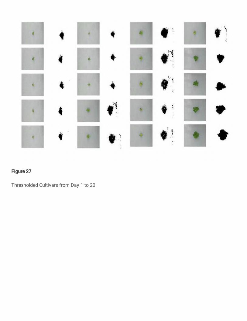
Figure 27

Thresholded Cultivars from Day 1 to 20

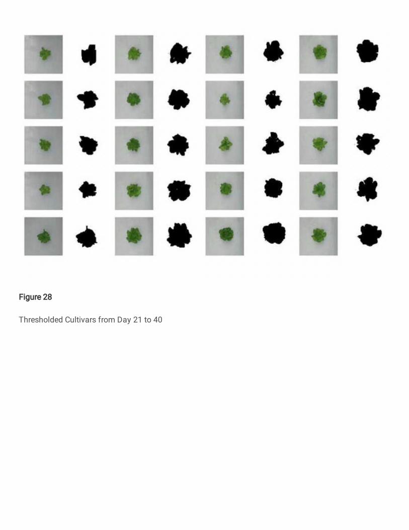
Figure 28

Thresholded Cultivars from Day 21 to 40

Figure 29

Thresholded Cultivars from Day 41 to 60

Figure 30

Thresholded Cultivars from Day 61 to 80

Figure 31

Formula used to calculate LAI RMSE on predicted outcome.

Figure 32

RMSE Compared to Ground LAI (Left) and Predicted LAI (Right)

Figure 33

Prediction summary of over 19 samples in test dataset

Figure 34

Plot comparing Ground Truth and predicted LAI values from EdgeImpulse Studio Model Testing section

Figure 35

LAI of segmented images

Figure 36

Compiled quantised binary for Regression model on Sony’s Spresense

Figure 37

Demonstrating various components used in the hardware system for Test Data Acquisition

Figure 38

Demonstrates distance between Camera and Plant for the model to work

Figure 39

Various images of live classi�cation and on-board processing algorithms

Figure 40

Battery Operated Telemetry system using SD card to store LAI predicted data