A Parallelization Scheme Based on Work Stealing for a class of SAT ...

A Parallelization Scheme Based on Work Stealing for a

class of SAT solvers

Bernard Jurkowiak, Chu Min Li and Gil UtardLaRIA, Universite de Picardie Jules Verne,33 rue Saint Leu, 80039 Amiens, FRANCEe-mail: {jurkowiak, cli, utard}@laria.u-picardie.fr

Abstract. Due to the inherent NP -completeness of SAT, many SAT problemscurrently cannot be solved in a reasonable time. Usually, to tackle a new class ofSAT problems, new ad-hoc algorithm must be designed. Another way to solve a newproblem is to use a generic solver and employ parallelism to reduce the solve time.

In this paper we propose a parallelization scheme for a class of SAT solvers basedon the DPLL procedure. The scheme uses dynamic load balancing mechanism basedon the work stealing techniques to deal with the irregularity of SAT problems. Weparallelize Satz, one of the best generic SAT solvers, with the scheme to obtain aparallel solver called PSatz. The first experimental results on random 3-SAT and aset of well-known structured problems show the efficiency of PSatz. PSatz is freelyavailable and runs on any networked workstations under Unix/Linux.

Keywords: automated theorem proving, SAT problem, parallelism

1. Introduction

Consider a propositional formula F in Conjunctive Normal Form(CNF) on a set of n boolean variables {x1, x2, · · · , xn}. A literal l isa variable xi or its negation xi, a clause c is a logical or of some literals(e.g. (x1 ∨ x2 ∨ x3)) and a formula F is a logical and of clauses. Ak-SAT problem is a problem where there are k literals per clause. Thesatisfiability (SAT) problem consists in finding an assignment of truthvalue (1 for true and 0 for false) to variables such that F is true. Ifsuch an assignment exists, then F is said satisfiable, otherwise, F issaid unsatisfiable.

SAT is a specific kind of finite-domain Constraint Satisfaction Prob-lem (CSP) and it is the first known NP -complete problem [4] (3-SATis its smallest NP -complete sub-problem).

Many problems in various domains can naturally be encoded intoSAT then solved by a SAT solver. Encoding a real-world problem intoSAT is generally easier than writing a specialized algorithm for theproblem. Moreover, some problems can be solved more efficiently bya SAT solver (after encoding) than by the specialized algorithm. Forexample, by using propositional reasoning, many problems like quasi-group completion problems [33, 35], planning [22, 21] and hardware

c© 2005 Kluwer Academic Publishers. Printed in the Netherlands.

Revue.tex; 25/01/2005; 16:42; p.1

2

modeling [10, 32] have already been solved with SAT solvers betterthan other methods.

As is pointed out by Selman, Kautz and McAllester in [30], severalother factors also contributed to the growing interest in SAT. First,new algorithms were developed such as WalkSAT [29], UnitWalk [15],SP [3], Sato [34], Satz [25], Chaff [28] and Kcnfs [9]. Second, continuousprogress in computer performance extends the range of the algorithms.Third, better encodings in SAT are found for interesting real-worldproblems.

However, because of the NP-completeness of SAT, we are in constantneed of more computing power to solve a significant range of SATproblems in reasonable time. Moreover, despite of the power of state-of-the-art SAT solvers, the proof of the satisfiability or the unsatisfiabilityof many interesting problems remains challenging (see e.g. [33]). Onthe other hand, single computers such as PC become so cheap that itis easy to find dozens of networked machines, providing considerablecomputing resources.

Thus, several distributed/parallel systematic SAT solvers have beendeveloped such as Bohm and Speckenmeyer Parallel Solver [2], PSATO[35], PaSAT [31] and PSolver [16] to exploit the power of networkedcomputers. In all these approaches, a formula is dynamically dividedinto subformulas which are then distributed among processors. Rela-tively small subformulas are sequentially solved by a processor. Whena processor begins to sequentially solve a subformula, it does not givepart of load of this solving to another processor.

The approaches work well in case subformulas of the same size re-quire roughly the same amount of time to be solved. Unfortunately,because of its NP -completeness, SAT is very irregular, because asubformula may require much more time to be solved than anothersubformula of the same size and this fact is currently unpredictable,especially when solving real-world problems. If the load balancing isnot preemptive and processors busy in (sequentially) solving hard sub-formulas cannot efficiently give part of their load to idle processors, idleprocessors cannot help busy ones and will remain idle after solving alleasy subformula.

In order to avoid the processor idleness, we propose in this paper anew approach to parallelize a class of SAT solvers. The load balancingis preemptive and idle processors steal parts of load of busy processorsfor load balancing. The approach is applied to parallelize Satz, one ofthe best generic solvers, to obtain an efficient systematic parallel SATsolver called PSatz (previously called //Satz in [20]).

The paper is organized as follows. We first present preliminariesabout the general arborescent search parallelization and SAT problems

Revue.tex; 25/01/2005; 16:42; p.2

3

with their search space in Section 2. Then we present Satz and someother DPLL procedures in section 3. In Section 4, we present our dy-namic load balancing scheme based on work stealing and its applicationto parallelize Satz. In Section 5, we show the performances of PSatzfor random 3-SAT problems and a set of well-known structured SATproblems. Finally we discuss related work and compare PSatz withother parallel solvers in Section 6 before concluding in Section 7.

2. Preliminaries

Our approach belongs to a large field of parallelization of arborescentsearch. In this section, we present some preliminaries in the field relatedto SAT problems and their search space.

2.1. Parallelization of an arborescent search

Many finite search spaces can be structured in form of a tree, of whicheach node represents a sub-space. An arborescent search consists invisiting every node of the tree in a specific order. For simplicity, weonly consider here depth first search in a finite binary tree, which isrecursively defined by

− visit the root

− search in the left subtree

− search in the right subtree

The tree may be known before the search or should dynamically beconstructed as the search proceeds.

Parallelization of an arborescent search consists in dividing thewhole task among p available processors, so that each processor carriesout roughly 1/p of the whole load. Ideally, the computation is p timesfaster. However, parallelization introduces some overhead (communica-tion, synchronization), so the speedup is generally smaller. Sometimes,we search for a single solution in the search space and the solution isin a subtree directly searched by a processor. In this case the speedupmay be larger than p. A speedup larger than p is said super-linear.

When all subtrees of a node are independent and roughly have thesame size, it is straightforward to parallelize the depth-first search, sincesearch(left-subtree) and search(right-subtree) can be simultaneouslyexecuted on two processors and each of the two searches can be inturn divided. The division continues until all processors are loaded. If

Revue.tex; 25/01/2005; 16:42; p.3

4

the subtrees have different size but the size of each subtree is knownor predictable, only larger subtrees are divided so that the load of eachprocessor is balanced.

When the subtrees of a node are of very different size but their sizecannot be predicted, we say the corresponding search problem is irreg-ular. Perfect load balancing cannot be obtained by a static partition ofthe tree among processors. In this case, a usual approach is to introducea dynamic load balancing scheme where the subtrees are redistributedduring the computation according to the load of different processors.

A dynamic load balancing scheme should allow to achieve two goals:the communication overhead between processors is as small as possibleand the load of processors is as balanced as possible. In other words,the overhead of redistribution should not be greater than the loadbalancing gain: redistributing too often may lead to a deteriorationof the efficiency.

When designing such a scheme, one essentially deals with thefollowing questions:

− When a redistribution must be fired?

− Which work must be redistributed?

− Which processors are elected to receive additional work?

These decisions are usually based on an estimation of the workloadand the cost of redistribution. Firing a redistribution may be due toan overload of a processor which then sends part of this work to a lessloaded processor. This technique is called Sender Initiative Decision(SID). Another technique is the Receiver Inititiative Decision (RID)where a less loaded processor asks task to a more loaded one. For heavycomputation, it was observed that RID strategy is usually better thanan SID one because fewer requests are initiated [36].

The search space of SAT problems can be naturally structured bya binary tree, the two subtrees of a node are separated by the truthvalue 1 and 0 (See subsection 2.4 below). However because of its NP -completeness, SAT is very irregular. We propose a RID approach inthis paper to parallelize a class of SAT solvers.

2.2. Depth cutoff and Ping-Pong phenomenon

When parallelizing an arborescent search (such as a depth-first search),a depth cutoff [14] is generally used to restrict the number of messagesexchanged between the processors, i.e., a processor does not give outa subtree at a depth greater than a fixed threshold. Search after this

Revue.tex; 25/01/2005; 16:42; p.4

5

threshold is then sequential. Adjusting the cutoff value is a challengingtask, since a small cutoff value limits the number of communicationsbut may increase processor idleness, and vice versa.

Adjusting the cutoff value for an irregular search problem such asSAT is still harder, because one cannot predict the size of subtrees afterthe cutoff threshold. Since a sequential search after the cutoff thresholdmay be very long, other processors may become idle after finishing allother tasks but cannot help the busy processor.

Standard depth cutoff is based on the number of workload partitionsalready done (i.e. partitions before the current node is reached) to de-cide whether the processor should divide the current subtree. A variantof depth cutoff technique uses an estimator to estimate the workloadof the current subtree, which is divided only if the estimated workloadis larger than a threshold.

Another difficulty when dealing with an irregular search problemis the so-called “Ping-Pong phenomenon”: the processors spend moretime in communication than in the search itself. In the extreme case, atask makes a round trip between two (or more) processors over and overas a ping-pong ball, processors spend no or little time on the searchitself.

2.3. SAT problems

SAT problems can be divided into two classes: random problems andstructured problems.

The most interesting random problems for us are random k-SAT.A random k-SAT problem of n variables and m clauses is generatedas follows. Each clause is created by randomly picking k variables andnegating each of them with probability 0.5. The case k = 3 is well stud-ied. It is found in [27] that when m/n is near 4.25, the 3-SAT problemsare the most difficult to solve and are satisfiable with probability 0.5.Random k-SAT problems are very suitable for studying the propertiesof SAT and for evaluating SAT solvers. We use hard random 3-SATproblems with m/n=4.25 in our experimentation.

While there is no intended relation between variables (and clauses)in a random problem, there may be different intended relations be-tween variables (and clauses) in a structured problem. Examples ofthese relations include symmetries (two variables are symmetric if theirpermutation in the formula gives the same formula) and equivalences(two literals are equivalent if their value is equal in all satisfying as-signments). Structured problems may come from the encoding of areal-world problem into SAT or may be created by hand according tosome properties.

Revue.tex; 25/01/2005; 16:42; p.5

6

For example, in order to encode into SAT the famous unsatisfiablepigeon hole problem of placing n + 1 pigeons in n holes so that everyhole exactly contains one pigeon [5], we number the pigeons from 1 ton + 1 and holes from 1 to n and define (n + 1)×n boolean variables asfollows:

xij =

{

1 if pigeon i is placed in hole j0 otherwise

We define a group of (n2+n+2)/2 clauses for each hole j (1 ≤ j ≤ n).The first clause of the group is:

x1j ∨ x2j ∨ ... ∨ xnj ∨ xn+1j

saying that hole j contains at least a pigeon. Then for every couple ofpigeons i1 and i2 (1 ≤ i1 < i2 ≤ n + 1), a clause xi1j ∨ xi2j is definedto say that these two pigeons cannot be both in hole j. The intendedmeaning of this group of clauses is that there is one and only one pigeonin hole j. We recall that the clauses in a random problem don’t haveany intended meaning.

The total number of clauses for this problem is (n3 + n2 + 2n)/2since there are n holes.

The boolean variables vector x1jx2j...xn+1j is symmetric to theboolean variables of x1kx2k...xn+1k for j 6= k, since if we simultaneouslypermute x1jx2j ...xn+1j with x1kx2k...xn+1k in the formula, we obtainthe same formula.

2.4. Search space of a SAT problem

There are 2n truth assignments in the search space for a SAT problemof n variables. Given any variable x, the search space can be dividedinto two sub-spaces. One sub-space contains all assignments in whichx=1, the other contains all assignments in which x=0. Each of thetwo sub-spaces can be in turn divided using another variable. So thewhole search space can be structured in a binary tree, of which eachleaf represents a disjoint sub-space specified by the partial assignmentfrom the root to the leaf.

For example, the binary tree in Figure 2 in section 4.1 structuresa search space into 5 sub-spaces respectively represented by 5 partialassignments (from left to right):

1. x1 = 1,

2. x1 = 0, x3 = 1,

3. x1 = 0, x3 = 0, x4 = 1, x5 = 1,

Revue.tex; 25/01/2005; 16:42; p.6

7

4. x1 = 0, x3 = 0, x4 = 1, x5 = 0,

5. x1 = 0, x3 = 0, x4 = 0

Each sub-space can be in turn structured by a (sub) binary tree.The DPLL procedure presented in the next section dynamically

structures the search space in a binary tree to solve SAT problems.

3. Satz and some other DPLL-based SAT solvers

SAT solvers can be divided into two classes:

− incomplete solvers that try to find a consistent assignment to afixed problem but are currently not designed to prove unsatisfia-bility;

− complete solvers that are able to find a consistent assignment andto prove unsatisfiability.

Most complete SAT solvers are based on the DPLL algorithm developedby Davis, Putnam, Logemann and Loveland [7, 6]. In this section after adescription of the DPLL procedure, we present some efficient completeDPLL-based solvers and justify our choice of parallelizing Satz.

3.1. The DPLL procedure

The DPLL procedure [7, 6] provides the basis of most completealgorithms for SAT. It is sketched in Algorithm 1.

In order to solve a SAT problem, the DPLL procedure dynamicallystructures a search space of all possible truth assignments into a bi-nary search tree until it either finds a satisfying truth assignment orconcludes that no such assignment exists. The recursive call in line10 of Algorithm 1 represents the left subtree (x = 1) in the binarysearch tree and the recursive call in line 13 represents the right subtree(x = 0). x is called branching variable. A leaf corresponds to an emptyclause (i.e. a dead-end) or to a satisfying assignment.

The DPLL algorithm is mainly based on the UnitPropagation pro-cedure (see lines 16-21), illustrated in the following example. Let F bethe following propositional formula:

F = (x1) ∧ (x1 ∨ x2) ∧ (x1 ∨ x3 ∨ x4) ∧ (x2 ∨ x5 ∨ x6) ∧ (x1 ∨ x6)

The first clause is unit since it contains only one literal. The Unit-Propagation procedure satisfies it by assigning x1 = 0, then it removes

Revue.tex; 25/01/2005; 16:42; p.7

8

all clauses containing x1 (which are satisfied) and reduces the clausescontaining x1 by removing x1 from them. The second clause becomingunit, the unit propagation continues by satisfying this new unit clauseand reducing the fourth clause. Finally, F becomes:

F = (x3 ∨ x4) ∧ (x5 ∨ x6)

Dividing a formula into two subformulas means that forsome x, we get two formulas F1=UnitPropagation(F ∧ (x)) andF2=UnitPropagation(F ∧ (x)).

Algorithm 1 DPLL procedure

1: DPLL(F)2: if F = ∅ then3: return “satisfiable”;4: end if5: F ← UnitPropagation(F);6: if F contains an empty clause then7: return “unsatisfiable”;8: end if9: choose x in F according to a heuristic H;

10: if DPLL(F ∧ (x)) = “satisfiable” then11: return “satisfiable”;12: else13: return DPLL(F ∧ (x));14: end if15:

16: UnitPropagation(F)17: while there is no empty clause and a unit clause with a literal l

exists in F do18: satisfy clauses containing l (remove them from F);19: reduce clauses containing l (remove l from them);20: end while21: return F ;

3.2. Satz

Satz is a DPLL procedure using a heuristic based on unit propaga-tion to select the next branching variable [26]. Given a variable x, theUnit Propagation heuristic examines x by adding, respectively, the unitclauses x and x to F and making independently two unit propagations.Let w(x) (resp. w(x)) be the number of clauses reduced by unit prop-agation when x (resp. x) is added into F . Then the following equation

Revue.tex; 25/01/2005; 16:42; p.8

9

suggested by Freeman [11] is used to give the weight of the variable x:

H(x) = w(x) ∗ w(x) ∗K + w(x) + w(x)

where K is a constant fixed experimentally.Satz branches on x such that H(x) is the largest. Intuitively, the

larger w(x) is, the more quickly DPLL(F∧(x)) may probably encountera contradiction. In this case DPLL(F ∧ (x)) produces a smaller tree.The equation H(x) favors those variables x such that w(x) and w(x) donot differ much. A consequence is that Satz constructs a very balancingbinary search tree for random problems [26].

Satz also includes the so-called experimental unit propagation of thesecond level [24] to eliminate small subtrees. The technique is based onthe following observation. If the satisfaction of a literal l introducesmany strong constraints (e.g. binary clauses) by unit propagation, itprobably leads to an imminent dead-end which can be detected byfurther experimental unit propagations.

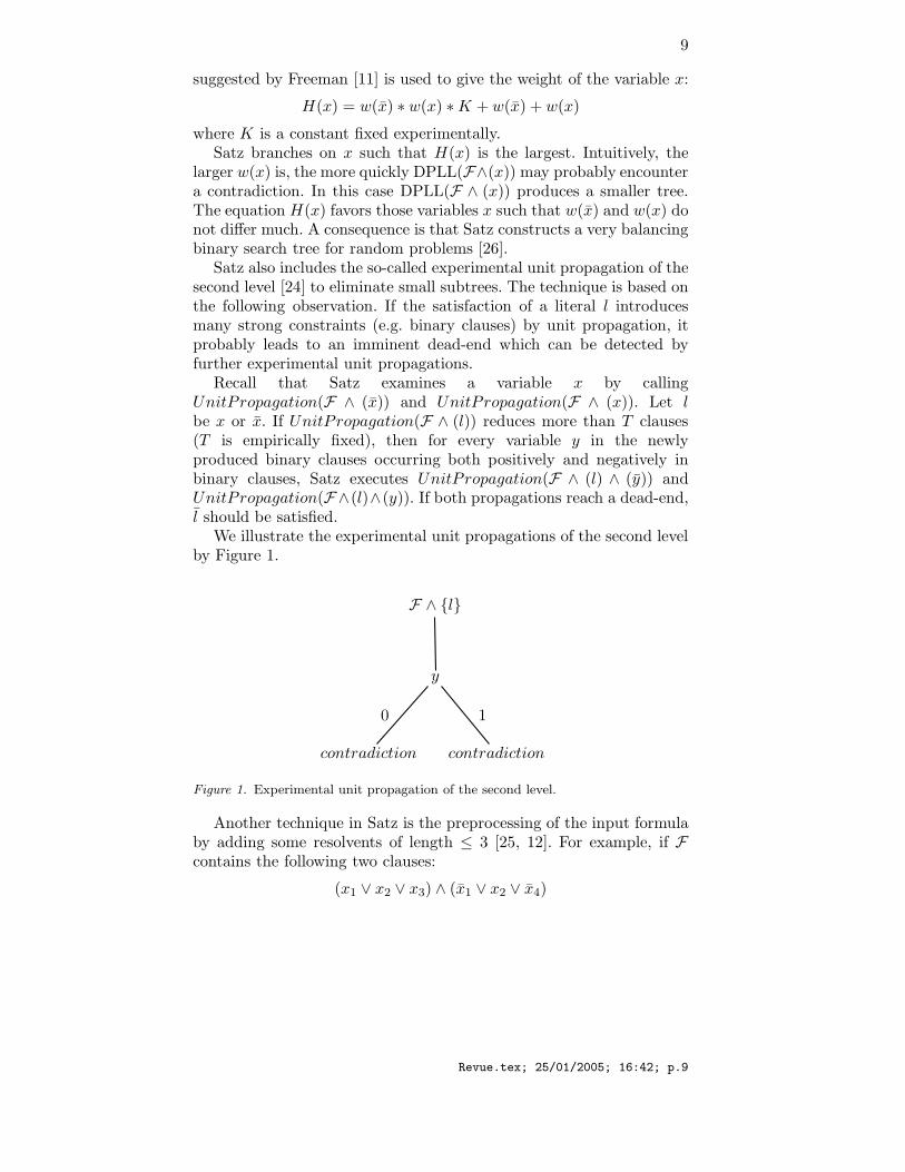
Recall that Satz examines a variable x by callingUnitPropagation(F ∧ (x)) and UnitPropagation(F ∧ (x)). Let lbe x or x. If UnitPropagation(F ∧ (l)) reduces more than T clauses(T is empirically fixed), then for every variable y in the newlyproduced binary clauses occurring both positively and negatively inbinary clauses, Satz executes UnitPropagation(F ∧ (l) ∧ (y)) andUnitPropagation(F∧(l)∧(y)). If both propagations reach a dead-end,l should be satisfied.

We illustrate the experimental unit propagations of the second levelby Figure 1.

F ∧ {l}

y

contradiction

0

contradiction

1

Figure 1. Experimental unit propagation of the second level.

Another technique in Satz is the preprocessing of the input formulaby adding some resolvents of length ≤ 3 [25, 12]. For example, if Fcontains the following two clauses:

(x1 ∨ x2 ∨ x3) ∧ (x1 ∨ x2 ∨ x4)

Revue.tex; 25/01/2005; 16:42; p.9

10

then the clause (x2∨x3∨x4) is added to F . The new clauses can in turnbe used to produce other resolvents. This process is performed untilsaturation. This preprocessing adds constraints in the input formula toexhibit contradiction more easily.

Many improved versions of Satz have been developed (e.g. [23]). Inthis paper, we parallelize Satz215 which includes the implied literalpropagation mechanism suggested by D. Le Berre [1]. Precisely, if bothF∧(x) and F ∧(x) implies a literal l, then l is satisfied and propagatedin F . This enables Satz to solve some hard real world problems [1, 18].

Thanks to these techniques, Satz is a generic SAT solver very effi-cient for hard random problems and many hard structured problems(see e.g. [1, 18, 26]). The source code of Satz is freely available [17].

3.3. Some other SAT solvers

There are many other efficient SAT solvers based on the DPLL proce-dure. Among the most representative SAT solvers, we find Sato [34],Chaff [28] and Kcnfs [8].

3.3.1. Sato and ChaffSato has been first developed to solve quasigroup problems. Then it hasbeen modified to solve structured problems such as DIMACS problems.Chaff is also developed to solve structured problems. One commonfeature of Sato and Chaff is the use of the so-called look-back searchtechniques.

Roughly speaking, when a DPLL-based SAT solver encounters adead-end in the left subtree, the look-back techniques analyze the rea-son of the dead-end. One or more clauses are added into the formulato avoid the same dead-end in the right subtree.

For example, suppose that the solver encounters an empty clausewhich is originally x1 ∨ x2 ∨ x3 (the clause becomes empty because x1,x2 and x3 are respectively assigned 0, 1 and 0) and that x1 is the lastassigned variable. If x1 is assigned 0 because x1 was in a unit clausewhich is originally x1 ∨ x4 ∨ x5 (x4 and x5 were assigned 0 before), thefalsification of x4 and x5 is the reason of x1=0. We replace x1 by x4∨x5

and obtain a new empty clause x4 ∨ x5 ∨ x2 ∨ x3. If the last assignedvariable in this new empty clause was in a unit clause, it is replaced byits reason to obtain another empty clause. The process continues untilthe last assigned variable is a branching variable. The DPLL procedurebranches on the other value of the branching variable.

Note that the empty clauses successively obtained become nonempty after backtracking. Look-back techniques add some of them intothe formula to prevent the solver from reaching the same dead-end in

Revue.tex; 25/01/2005; 16:42; p.10

11

the right subtree, since these clauses would become empty before theclause x1 ∨ x2 ∨ x3 in the right subtree.

Obviously, the left and right subtrees are not independent for solversemploying look-back techniques, which makes it harder to parallelizethem.

3.3.2. KcnfsKcnfs is specially developed to solve random k-SAT problems. It uses apowerful heuristic exploiting the random properties of k-SAT to choosethe next branching variable. It is very efficient for k-SAT problems. Nolook-back techniques are used in Kcnfs.

3.4. Comparison of Satz, Kcnfs, Sato and Chaff

We compare the performance of Satz, Kcnfs, Sato and Chaff for random3-SAT problems and several representative structured SAT problemson a PC with an Athlon XP2000+ CPU and 256Mb of RAM underLinux.

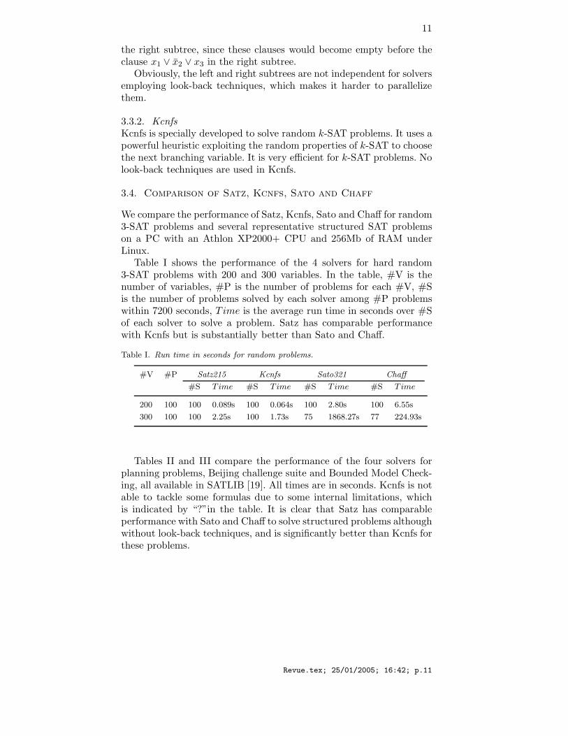
Table I shows the performance of the 4 solvers for hard random3-SAT problems with 200 and 300 variables. In the table, #V is thenumber of variables, #P is the number of problems for each #V, #Sis the number of problems solved by each solver among #P problemswithin 7200 seconds, T ime is the average run time in seconds over #Sof each solver to solve a problem. Satz has comparable performancewith Kcnfs but is substantially better than Sato and Chaff.

Table I. Run time in seconds for random problems.

#V #P Satz215 Kcnfs Sato321 Chaff

#S T ime #S T ime #S T ime #S T ime

200 100 100 0.089s 100 0.064s 100 2.80s 100 6.55s

300 100 100 2.25s 100 1.73s 75 1868.27s 77 224.93s

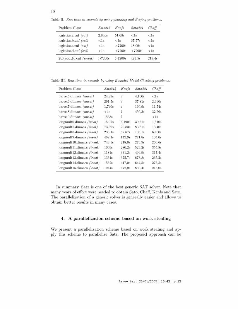
Tables II and III compare the performance of the four solvers forplanning problems, Beijing challenge suite and Bounded Model Check-ing, all available in SATLIB [19]. All times are in seconds. Kcnfs is notable to tackle some formulas due to some internal limitations, whichis indicated by “?”in the table. It is clear that Satz has comparableperformance with Sato and Chaff to solve structured problems althoughwithout look-back techniques, and is significantly better than Kcnfs forthese problems.

Revue.tex; 25/01/2005; 16:42; p.11

12

Table II. Run time in seconds by using planning and Beijing problems.

Problem Class Satz215 Kcnfs Sato321 Chaff

logistics.a.cnf (sat) 2.840s 51.08s <1s <1s

logistics.b.cnf (sat) <1s <1s 37.57s <1s

logistics.c.cnf (sat) <1s >7200s 18.09s <1s

logistics.d.cnf (sat) <1s >7200s >7200s <1s

2bitadd 10.cnf (unsat) >7200s >7200s 493.5s 219.4s

Table III. Run time in seconds by using Bounded Model Checking problems.

Problem Class Satz215 Kcnfs Sato321 Chaff

barrel5.dimacs (unsat) 24,99s ? 4,100s <1s

barrel6.dimacs (unsat) 291,5s ? 37,81s 2,690s

barrel7.dimacs (unsat) 1,740s ? 160,9s 11,74s

barrel8.dimacs (unsat) <1s ? 450,3s 32,56s

barrel9.dimacs (unsat) 1563s ? <1s

longmult6.dimacs (insat) 15,07s 6,190s 39,51s 1,510s





longmult11.dimacs (insat) 1009s 280,2s 529,2s 355,8s





In summary, Satz is one of the best generic SAT solver. Note thatmany years of effort were needed to obtain Sato, Chaff, Kcnfs and Satz.The parallelization of a generic solver is generally easier and allows toobtain better results in many cases.

4. A parallelization scheme based on work stealing

We present a parallelization scheme based on work stealing and ap-ply this scheme to parallelize Satz. The proposed approach can be

Revue.tex; 25/01/2005; 16:42; p.12

13

directly used to parallelize any DPLL-based solver without look-backtechniques.

4.1. Representation of working context of the DPLL

procedure

We recall that the DPLL procedure dynamically structures the wholesearch space into a binary search tree to solve a SAT problem. At anymoment of the search, the DPLL procedure is at a tree node and isgoing to construct the two subtrees rooted at this node. We representa node by a context in which we want to find three things:

− the part of the tree that has been constructed and explored,

− the current partial variable assignment,

− the part of the tree remaining to construct.

For this purpose we define the context by an ordered list of triplets:

(variable, current value, remaining value)

where:

current value =

{

1 (true)0 (false)

and:

remaining value =

1 (true)0 (false)−1 (no more remaining value to try)

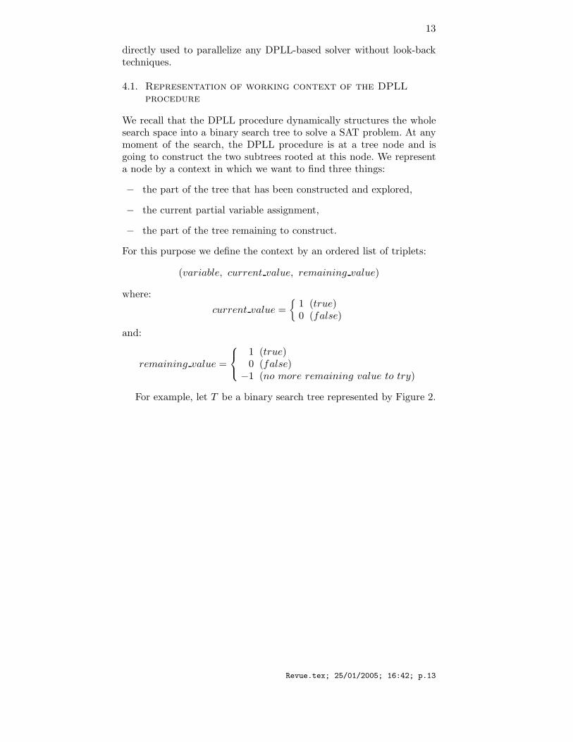
For example, let T be a binary search tree represented by Figure 2.

Revue.tex; 25/01/2005; 16:42; p.13

14

...

...

1

3

4

5

1

01

01

0

... : Explored subtree

: Current node

: Remaining subtree root

x

x

x

x01

Figure 2. A binary search tree T and its contexts.

T divides the whole search space in 5 disjoint subspaces (see section2.4). The current node (or subspace) of T is represented by the followinglist of triplets:

{(x1, 0,−1), (x3, 0,−1), (x4, 1, 0), (x5 , 1, 0)}.

From the context, we know that the DPLL procedure has succes-sively explored the subspaces (or subtrees) respectively represented bythe following partial assignments:

{(x1 = 1)}

{(x1 = 0), (x3 = 1)}

since the remaining-value -1 in the context of the current node meansthat the truth value opposit to the current one has been tried out (un-sucessfully) already. The subspaces (or subtrees) remaining to exploreare respectively represented by the partial assignments:

x1 = 0, x3 = 0, x4 = 1, x5 = 0

and:x1 = 0, x3 = 0, x4 = 0

and correspond to the contexts (assume that the first subspace isexplored before the second one):

{(x1, 0,−1), (x3, 0,−1), (x4, 1, 0), (x5, 0,−1)}

{(x1, 0,−1), (x3, 0,−1), (x4, 0,−1)}

Since a context represents the current partial assignment, the vari-ables fixed (i.e. assigned) by unit propagation are also included (in

Revue.tex; 25/01/2005; 16:42; p.14

15

order) with remaining-value -1. In a context, we do not distinguish abranching variable with remaining-value -1 and a variable fixed by unitpropagation. For example, x3 in the above context might be a variablefixed by unit propagation.

A natural way to parallelize the DPLL procedure is to exploit theinherent parallelism exposed by the tree. Indeed, each subtree can beexplored independently. On a parallel computer with P processors, itis straightforward to divide the binary search tree in P subtrees andassigns each subtree to a processor. However, since the workloads ofthese subtrees are very different but are currently unpredictable, thehard issue is to design a dynamic load balancing so that the communi-cation overhead is as small as possible and the load of each processoris as balanced as possible.

We present below our approach to parallelize Satz. The basic ideais that an idle processor steals one of the remaining subtrees of a busyprocessor.

4.2. General communication model

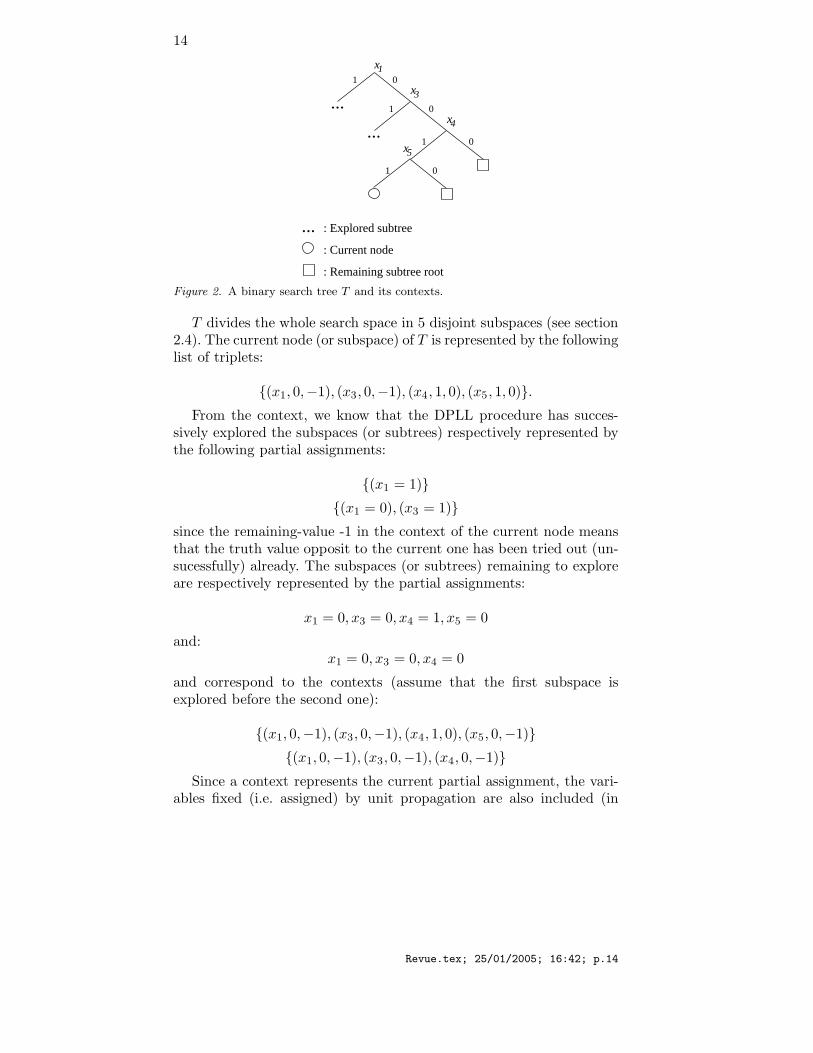
We choose the master/slave architecture for communication. As is il-lustrated in Figure 3, every processes (master or slave) has two threads:working thread and communicating thread. The communicating threadreceives messages and puts them into its letter-box.

The working thread of a slave is a normal Satz procedure, butmodified for communication. By a semaphore mechanism, it detectsand reads its messages from the letter-box before every splitting. Notethat all slaves use the same heuristic to select branching variable forsplitting.

BOSS

BOSS : Master working thread

: Communicating thread

: Satz thread

Figure 3. Master-Slave model.

Revue.tex; 25/01/2005; 16:42; p.15

16

4.3. Initialization

The master initiates the computation by launching all slaves. Each slavegets the same input formula and pre-processes it before being ready.Then the master choose an arbitrary ready processor and makes itsworking thread start the whole computation. At this stage, there is abusy slave and other ready processors are idle.

4.4. Dynamic load balancing

When one or several slaves are idle after the preprocessing or afterfinishing their subtree, they send a task request to the master. Themaster asks the load of each busy slave and removes the first remainingsubtree of the most loaded slave and sends it to an idle slave. The loadevaluation is carried out in the following manner.

Consider the context of a slave:

{(x1, cv1, rv1), (x2, cv2, rv2), ..., (xk , cvk, rvk)}

where cvk is the (current) value of xk in the current partial assignment,rvk is the remaining value of xk to be tried, the position of the firstremaining subtree is the smallest j (1 ≤ j ≤ k) such that rvj is differentfrom -1. Intuitively, the larger j is, the more variables are fixed in thecontext:

{(x1, cv1,−1), (x2, cv2,−1), ..., (xj−1, cvj−1,−1), (xj , cvj , rvj)}

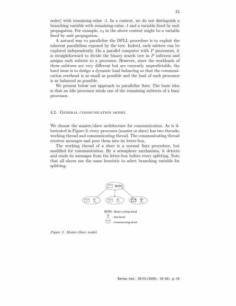
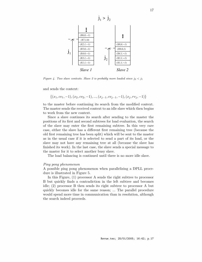
In this case, the corresponding remaining subtree will probably besmaller. Figure 4 shows an example. The slave with the smallest posi-tion j of the first remaining subtree is said the most loaded. If there areat least two most loaded slaves, the positions of the second remainingsubtrees of these slaves are compared. The remaining ties are brokenarbitrarily.

The master begins load balancing by asking all busy slaves to sendthe positions of their first and second remaining subtrees. A specialvalue is sent for the case where there are no remaining subtrees in thecontext and the case where there is only one remaining subtree. Thenthe master selects the most loaded slave and sends it a stealing messageto get its first remaining tree.

After sending the positions of its first and second remaining subtrees,a slave continues its search. If slave i is selected and its first remainingsubtree is at position j, it modifies its context into:

{(x1, cv1,−1), ..., (xj , cvj ,−1),(xj+1, cvj+1, rvj+1), ..., (xk , cvk, rvk)}

Revue.tex; 25/01/2005; 16:42; p.16

17

.

.

.

.

.

.

>

Slave 1 Slave 2

(X6,0,−1)

(X7,1,0)

(X2,1,−1)

(X5,0,−1)

(X4,0,−1)

(X3,1,−1)

(X8,0,−1)

(X9,0,1)

(X4,1,−1)

(X3,1,−1)

(X1,1,−1)(X1,1,−1)

j j1 2

j1

j2

Figure 4. Two slave contexts. Slave 2 is probably more loaded since j2 < j1

and sends the context:

{(x1, cv1,−1), (x2, cv2,−1), ..., (xj−1, cvj−1,−1), (xj , rvj,−1)}

to the master before continuing its search from the modified context.The master sends the received context to an idle slave which then beginsto work from the new context.

Since a slave continues its search after sending to the master thepositions of its first and second subtrees for load evaluation, the searchof the slave may enter the first remaining subtree. In this very rarecase, either the slave has a different first remaining tree (because theold first remaining tree has been split) which will be sent to the masteras in the usual case if it is selected to send a part of its load, or theslave may not have any remaining tree at all (because the slave hasfinished its work). In the last case, the slave sends a special message tothe master for it to select another busy slave.

The load balancing is continued until there is no more idle slave.

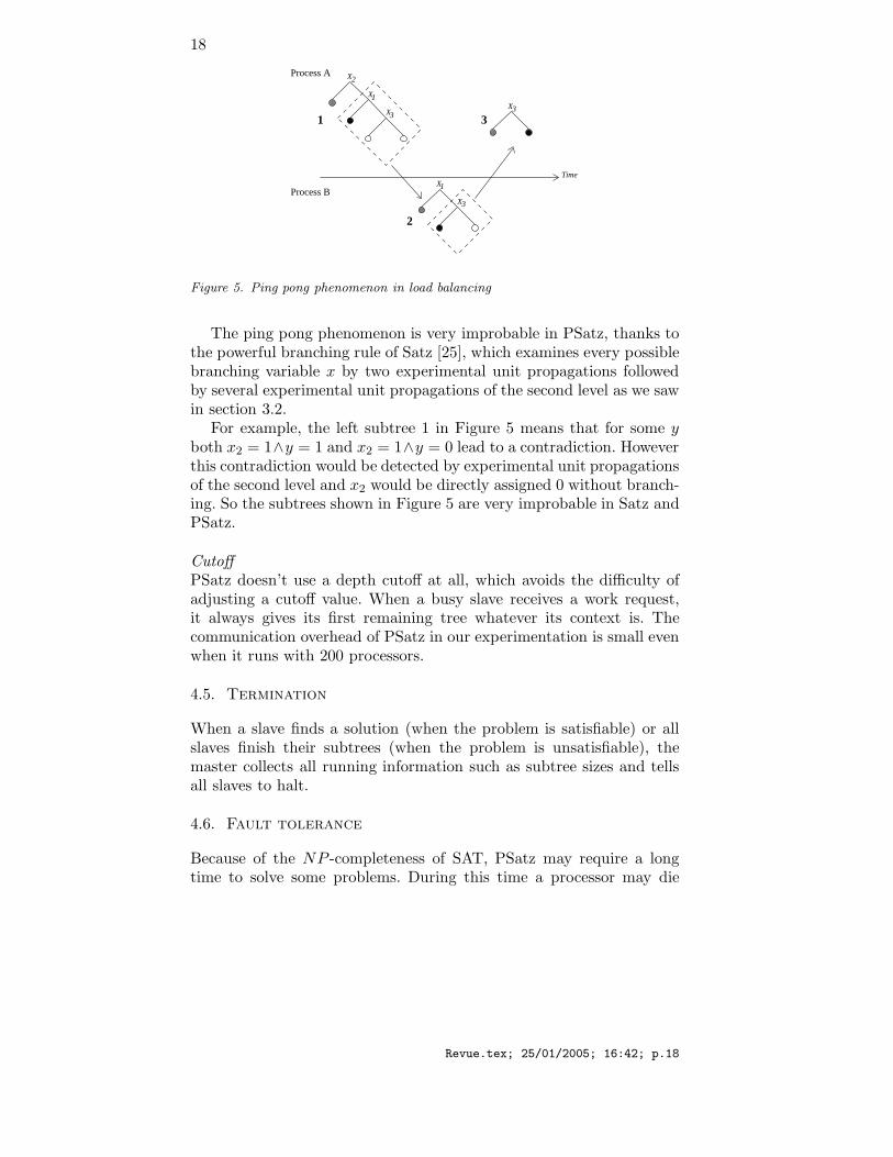
Ping pong phenomenonA possible ping pong phenomenon when parallelizing a DPLL proce-dure is illustrated in Figure 5.

In this Figure, (1) processor A sends the right subtree to processorB but quickly finds a contradiction in the left subtree and becomesidle; (2) processor B then sends its right subtree to processor A butquickly becomes idle for the same reason; ... The parallel procedurewould spend more time in communication than in resolution, althoughthe search indeed proceeds.

Revue.tex; 25/01/2005; 16:42; p.17

18

Time

1 3

2

Process A

Process B

X1

X3

X

X

X

X2

1

3

3

Figure 5. Ping pong phenomenon in load balancing

The ping pong phenomenon is very improbable in PSatz, thanks tothe powerful branching rule of Satz [25], which examines every possiblebranching variable x by two experimental unit propagations followedby several experimental unit propagations of the second level as we sawin section 3.2.

For example, the left subtree 1 in Figure 5 means that for some yboth x2 = 1∧y = 1 and x2 = 1∧y = 0 lead to a contradiction. Howeverthis contradiction would be detected by experimental unit propagationsof the second level and x2 would be directly assigned 0 without branch-ing. So the subtrees shown in Figure 5 are very improbable in Satz andPSatz.

CutoffPSatz doesn’t use a depth cutoff at all, which avoids the difficulty ofadjusting a cutoff value. When a busy slave receives a work request,it always gives its first remaining tree whatever its context is. Thecommunication overhead of PSatz in our experimentation is small evenwhen it runs with 200 processors.

4.5. Termination

When a slave finds a solution (when the problem is satisfiable) or allslaves finish their subtrees (when the problem is unsatisfiable), themaster collects all running information such as subtree sizes and tellsall slaves to halt.

4.6. Fault tolerance

Because of the NP -completeness of SAT, PSatz may require a longtime to solve some problems. During this time a processor may die

Revue.tex; 25/01/2005; 16:42; p.18

19

and/or the network may be interrupted. Fault tolerance means that theresolution should be continued if one or more slaves die, and that theresolution can be stopped and re-started from the interruption point.

In our approach, all slaves send their current context to the masterto be saved every hour. After a load balancing, the master also savesthe new context of the two concerned slaves. If a slave dies, the mastersends its saved context to the idle slave at the time of load balancingso that the work of the died slave can be continued.

It seems that one hour is a good time interval in our experimenta-tion, since it only produces negligible communication overhead and thedeath of a slave causes at most the loss of one hour computation.

Our fault tolerance mechanism is similar to that implemented inPSATO [35].

4.7. Implementation

We implemented PSatz in the C language using RPC (Remote Proce-dure Call) and Posix Threads, which are standard. Therefore, PSatzruns on any networked machines under Linux (Unix) without specifictoolkit. PSatz is available at the following url:

http://www.laria.u-picardie.fr/∼cli/englishpage.html

5. Performance evaluation

We use random 3-SAT problems and a set of well-known structuredreal-world problems to evaluate the performances of PSatz. Our ex-perimental results are obtained on a cluster of 216 computers (HPe-vectra nodes with Pentium III 733 MHZ processors and 256 Mb ofRAM) under Linux (Linux kernel 2.2.15-4mdk or Linux kernel 2.4.2)and networked by Fast-Ethernet (100 Mbit/second) and 5 switches (HPprocurve 4000 with 1 Gbits/second switch mesh) called Icluster1.

All communication times are in seconds and represent the totaltime the master spends for sending messages to slaves (including workrequests and contexts). The time for the master to send one messageis measured from the point the master sends the message to a slave tothe point the master receives the acknowledgment of receipt from theslave.

All run times are also in seconds, unless otherwise stated, and rep-resent real times of the master starting from the reading of the inputformula to the end of the resolution. This time includes the commu-nication time of the master, load evaluation times and computation

1 http://www-id.imag.fr/Grappes/icluster/description.html

Revue.tex; 25/01/2005; 16:42; p.19

20

time of the slave that terminates last for unsatisfiable problem or thecomputation time of the slave that finds a model first plus the timeto halt all other slaves and the master for satisfiable problem. PSatzuses NFS (Network File System): at the beginning all processors readand pre-process simultaneously the input formula. Note that, Satz andPSatz develop the same tree for unsatisfiable problems because theyuse the same heuristic for branching.

5.1. Random 3-SAT problems

We show the performance of PSatz for hard random 3-SAT problems.We generate 100 problems with 400, 450, 500 variables, respectively, 25problems with 550 variables and 20 problems with 600 variables, andseparate results for satisfiable and unsatisfiable problems.

In the following Tables, #V is the number of variables, #P is thenumber of solved problems, T1 is the average real time for sequentialSatz, T128 is the average real time for PSatz on 128 processors, Sp isthe Speedup T1/T128, #WB is the average number of load balancings(after the initialization) and Tcom is the average total communicationtime spent by PSatz (note that Tcom is included in T128). Standarddeviation is noted by (std dev.).

Note also that, the average is taken over #P. For example, theaverage real time of Satz is Ttotal/#P where Ttotal is the total realtime for all the #P instances.

5.1.1. Unsatisfiable random 3-SAT problemsTables IV and V show the performance of PSatz on unsatisfiable ran-dom 3-SAT problems on 128 processors for problems with 400, 450 and500 variables.

The speedup of PSatz is smaller for easier problems, because thecommunication overhead for load balancing is relatively more impor-tant for them. For example, the average communication time of PSatzrepresents 18.21 % of the real time for problems with 400 variables, butthe part of the communication is reduced to 2.18 % for problems with500 variables. Despite the number of load balance operations is moreimportant for larger problems, the communication time measured forthese problems is negligible compared to the real time.

The reading and the pre-processing of the input formula by all slavesis not negligible compared to the search time for small problems, whichis the second reason for the smaller speedup of PSatz for these problems.

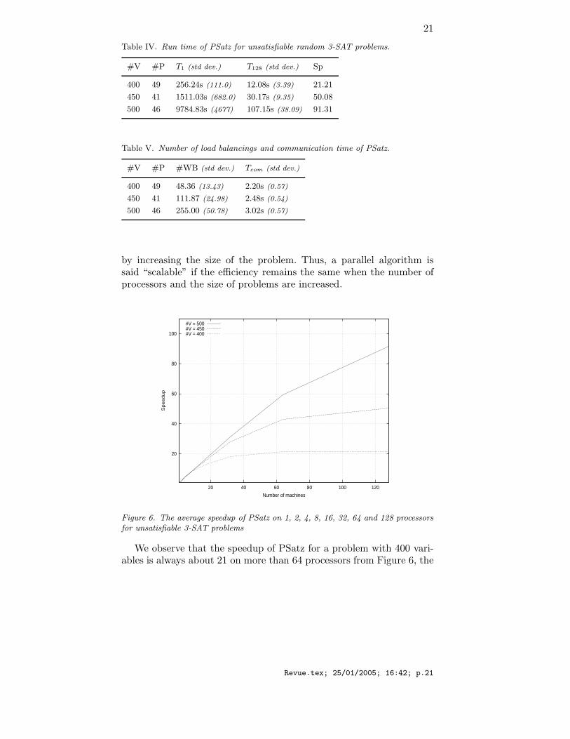
Figure 6 shows the scalability of PSatz. Usually when the numberof processors increases, the overhead of communications increases too.To keep a good efficiency, it is necessary to compensate this overhead

Revue.tex; 25/01/2005; 16:42; p.20

21

Table IV. Run time of PSatz for unsatisfiable random 3-SAT problems.

#V #P T1 (std dev.) T128 (std dev.) Sp

400 49 256.24s (111.0) 12.08s (3.39) 21.21

450 41 1511.03s (682.0) 30.17s (9.35) 50.08

500 46 9784.83s (4677) 107.15s (38.09) 91.31

Table V. Number of load balancings and communication time of PSatz.

#V #P #WB (std dev.) Tcom (std dev.)

400 49 48.36 (13.43) 2.20s (0.57)

450 41 111.87 (24.98) 2.48s (0.54)

500 46 255.00 (50.78) 3.02s (0.57)

by increasing the size of the problem. Thus, a parallel algorithm issaid “scalable” if the efficiency remains the same when the number ofprocessors and the size of problems are increased.

20

40

60

80

100

20 40 60 80 100 120

Sp

ee

du

p

Number of machines

#V = 500#V = 450#V = 400

Figure 6. The average speedup of PSatz on 1, 2, 4, 8, 16, 32, 64 and 128 processorsfor unsatisfiable 3-SAT problems

We observe that the speedup of PSatz for a problem with 400 vari-ables is always about 21 on more than 64 processors from Figure 6, the

Revue.tex; 25/01/2005; 16:42; p.21

22

communication overhead cancels the benefit of the increase in processornumber for these easy problems. The phenomenon suggests a limit ofthe performance of the parallelization, to be studied in the future.However we observe in Figure 6 that PSatz is indeed scalable, sincefor a fixed number of processors, the efficiency of the parallelizationincreases with the size of problems.

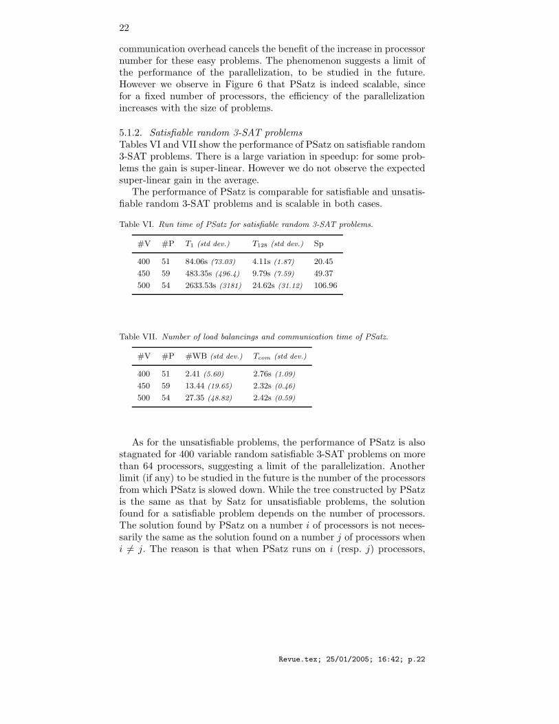
5.1.2. Satisfiable random 3-SAT problemsTables VI and VII show the performance of PSatz on satisfiable random3-SAT problems. There is a large variation in speedup: for some prob-lems the gain is super-linear. However we do not observe the expectedsuper-linear gain in the average.

The performance of PSatz is comparable for satisfiable and unsatis-fiable random 3-SAT problems and is scalable in both cases.

Table VI. Run time of PSatz for satisfiable random 3-SAT problems.

#V #P T1 (std dev.) T128 (std dev.) Sp

400 51 84.06s (73.03) 4.11s (1.87) 20.45

450 59 483.35s (496.4) 9.79s (7.59) 49.37

500 54 2633.53s (3181) 24.62s (31.12) 106.96

Table VII. Number of load balancings and communication time of PSatz.

#V #P #WB (std dev.) Tcom (std dev.)

400 51 2.41 (5.60) 2.76s (1.09)

450 59 13.44 (19.65) 2.32s (0.46)

500 54 27.35 (48.82) 2.42s (0.59)

As for the unsatisfiable problems, the performance of PSatz is alsostagnated for 400 variable random satisfiable 3-SAT problems on morethan 64 processors, suggesting a limit of the parallelization. Anotherlimit (if any) to be studied in the future is the number of the processorsfrom which PSatz is slowed down. While the tree constructed by PSatzis the same as that by Satz for unsatisfiable problems, the solutionfound for a satisfiable problem depends on the number of processors.The solution found by PSatz on a number i of processors is not neces-sarily the same as the solution found on a number j of processors wheni 6= j. The reason is that when PSatz runs on i (resp. j) processors,

Revue.tex; 25/01/2005; 16:42; p.22

23

i (resp. j) disjoint subspaces are simultaneously searched, we do notknow how to predict which subspace contains a solution and when thesolution is reached.

20

40

60

80

100

20 40 60 80 100 120

Sp

ee

du

p

Number of machines

#V = 500#V = 450#V = 400

Figure 7. The average speedup of PSatz on 1, 2, 4, 8, 16, 32, 64 and 128 processorsfor satisfiable random 3-SAT problems

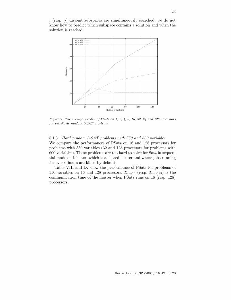
5.1.3. Hard random 3-SAT problems with 550 and 600 variablesWe compare the performances of PSatz on 16 and 128 processors forproblems with 550 variables (32 and 128 processors for problems with600 variables). These problems are too hard to solve for Satz in sequen-tial mode on Icluster, which is a shared cluster and where jobs runningfor over 6 hours are killed by default.

Table VIII and IX show the performance of PSatz for problems of550 variables on 16 and 128 processors. Tcom16 (resp. Tcom128) is thecommunication time of the master when PSatz runs on 16 (resp. 128)processors.

Revue.tex; 25/01/2005; 16:42; p.23

24

Table VIII. Run time of PSatz for problems of 550 variables.

#V #P T16 T128 T16/T128 #WB128

Unsat 550 12 2743.50s 377.75s 7.26 411.75

Sat 550 13 839.76s 145.53s 5.77 41.53

Table IX. Communication time of PSatz for problems of 550 variables.

#V #P Tcom16 Tcom128

Unsat 550 12 2.41s 3.66s

Sat 550 13 1.61s 2.53s

Figure 8 shows the efficiency of PSatz for problems of 550 variables.It appears that PSatz has a linear speedup on 16, 32, 64 and 128processors for these problems.

1

2

3

4

5

6

7

8

20 40 60 80 100 120

Spee

dup

Number of machines

UnsatisfiableSatisfiable

Figure 8. The average speedup of PSatz compared with 16 processors for hard random3-SAT problems of 550 variables on 16, 32, 64 and 128 processors.

Table X and XI show the performance of PSatz for problems with600 variables. Tcom32 is the communication time of the master whenPSatz runs on 32 processors.

Revue.tex; 25/01/2005; 16:42; p.24

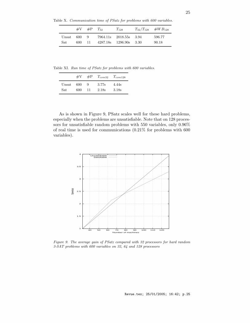
25

Table X. Communication time of PSatz for problems with 600 variables.

#V #P T32 T128 T32/T128 #WB128

Unsat 600 9 7964.11s 2018.55s 3.94 596.77

Sat 600 11 4287.18s 1296.90s 3.30 90.18

Table XI. Run time of PSatz for problems with 600 variables.

#V #P Tcom32 Tcom128

Unsat 600 9 3.77s 4.44s

Sat 600 11 2.18s 3.18s

As is shown in Figure 9, PSatz scales well for these hard problems,especially when the problems are unsatisfiable. Note that on 128 proces-sors for unsatisfiable random problems with 550 variables, only 0.96%of real time is used for communications (0.21% for problems with 600variables).

1

1.5

2

2.5

3

3.5

4

40 50 60 70 80 90 100 110 120

Spee

dup

Number of machines

UnsatisfiableSatisfiable

Figure 9. The average gain of PSatz compared with 32 processors for hard random3-SAT problems with 600 variables on 32, 64 and 128 processors

Revue.tex; 25/01/2005; 16:42; p.25

26

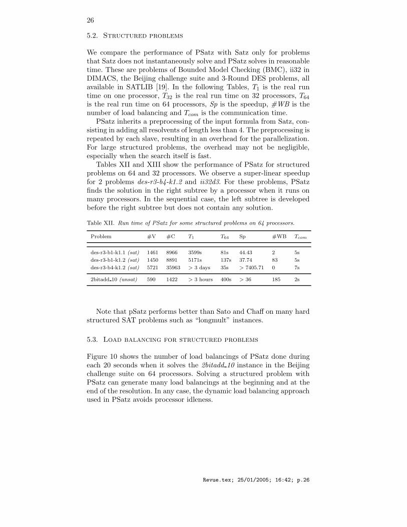
5.2. Structured problems

We compare the performance of PSatz with Satz only for problemsthat Satz does not instantaneously solve and PSatz solves in reasonabletime. These are problems of Bounded Model Checking (BMC), ii32 inDIMACS, the Beijing challenge suite and 3-Round DES problems, allavailable in SATLIB [19]. In the following Tables, T1 is the real runtime on one processor, T32 is the real run time on 32 processors, T64

is the real run time on 64 processors, Sp is the speedup, #WB is thenumber of load balancing and Tcom is the communication time.

PSatz inherits a preprocessing of the input formula from Satz, con-sisting in adding all resolvents of length less than 4. The preprocessing isrepeated by each slave, resulting in an overhead for the parallelization.For large structured problems, the overhead may not be negligible,especially when the search itself is fast.

Tables XII and XIII show the performance of PSatz for structuredproblems on 64 and 32 processors. We observe a super-linear speedupfor 2 problems des-r3-b4-k1.2 and ii32d3. For these problems, PSatzfinds the solution in the right subtree by a processor when it runs onmany processors. In the sequential case, the left subtree is developedbefore the right subtree but does not contain any solution.

Table XII. Run time of PSatz for some structured problems on 64 processors.

Problem #V #C T1 T64 Sp #WB Tcom

des-r3-b1-k1.1 (sat) 1461 8966 3599s 81s 44.43 2 5s

des-r3-b1-k1.2 (sat) 1450 8891 5171s 137s 37.74 83 5s

des-r3-b4-k1.2 (sat) 5721 35963 > 3 days 35s > 7405.71 0 7s

2bitadd 10 (unsat) 590 1422 > 3 hours 400s > 36 185 2s

Note that pSatz performs better than Sato and Chaff on many hardstructured SAT problems such as “longmult” instances.

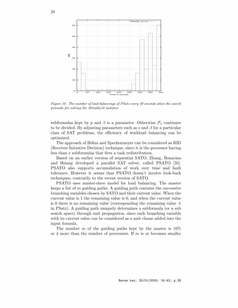
5.3. Load balancing for structured problems

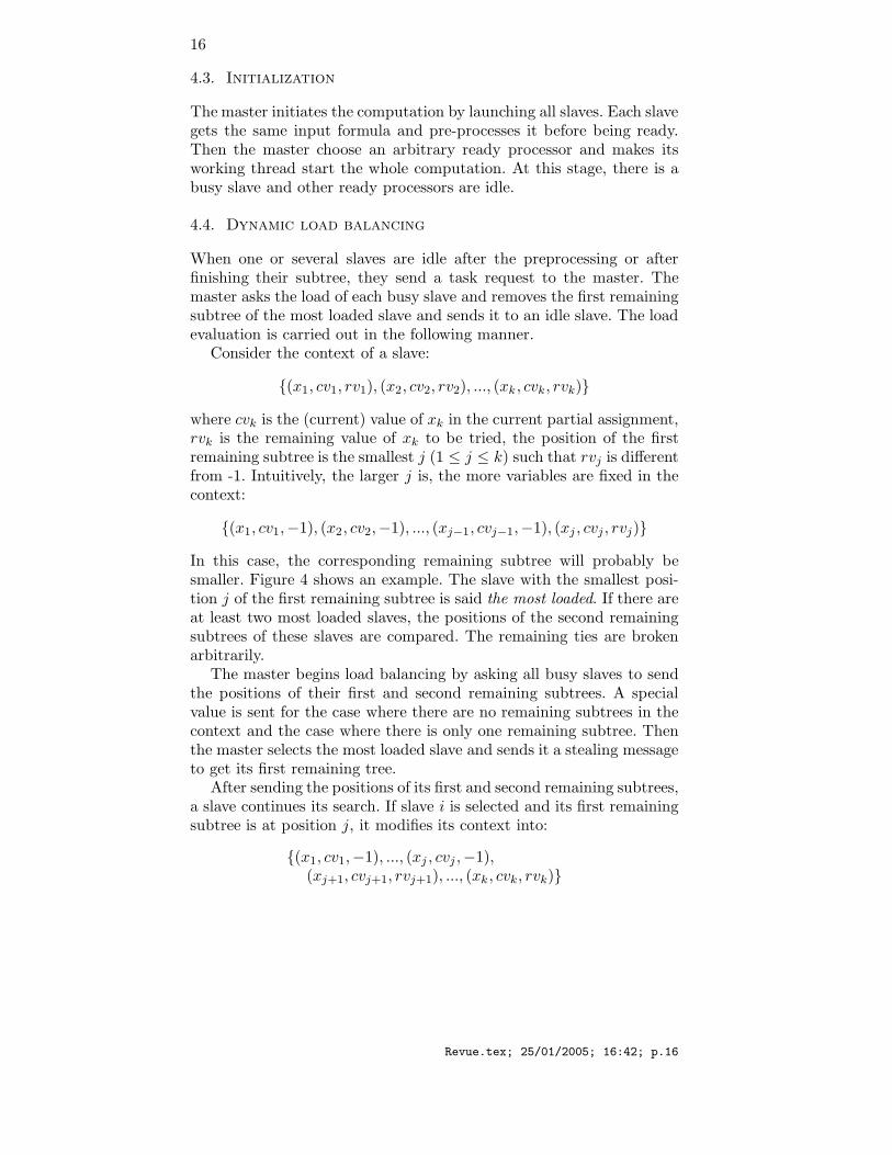
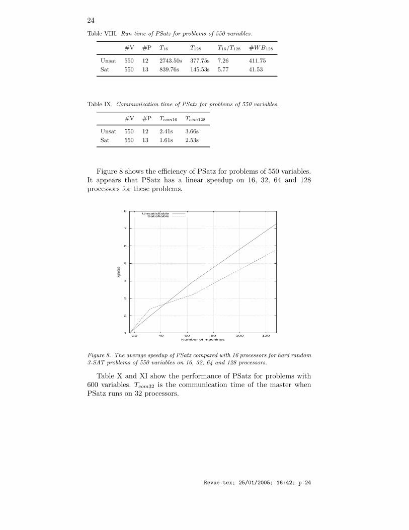
Figure 10 shows the number of load balancings of PSatz done duringeach 20 seconds when it solves the 2bitadd 10 instance in the Beijingchallenge suite on 64 processors. Solving a structured problem withPSatz can generate many load balancings at the beginning and at theend of the resolution. In any case, the dynamic load balancing approachused in PSatz avoids processor idleness.

Revue.tex; 25/01/2005; 16:42; p.26

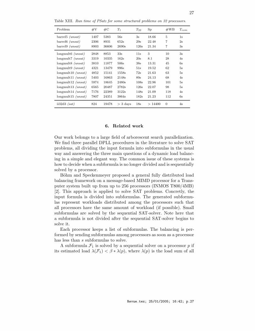
27

Table XIII. Run time of PSatz for some structured problems on 32 processors.

Problem #V #C T1 T32 Sp #WB Tcom

barrel5 (unsat) 1407 5383 56s 3s 18.66 5 1s

barrel6 (unsat) 2306 8931 652s 29s 22.48 7 2s

barrel9 (unsat) 8903 36606 2690s 126s 21.34 7 3s

longmult6 (unsat) 2848 8853 33s 11s 3 10 3s

longmult7 (unsat) 3319 10335 162s 20s 8.1 28 4s









ii32d3 (sat) 824 19478 > 3 days 18s > 14400 0 4s

6. Related work

Our work belongs to a large field of arborescent search parallelization.We find three parallel DPLL procedures in the literature to solve SATproblems, all dividing the input formula into subformulas in the usualway and answering the three main questions of a dynamic load balanc-ing in a simple and elegant way. The common issue of these systems ishow to decide when a subformula is no longer divided and is sequentiallysolved by a processor.

Bohm and Speckenmeyer proposed a general fully distributed loadbalancing framework on a message-based MIMD processor for a Trans-puter system built up from up to 256 processors (INMOS T800/4MB)[2]. This approach is applied to solve SAT problems. Concretly, theinput formula is divided into subformulas. The generated subformu-las represent workloads distributed among the processors such thatall processors have the same amount of workload (if possible). Smallsubformulas are solved by the sequential SAT-solver. Note here thata subformula is not divided after the sequential SAT-solver begins tosolve it.

Each processor keeps a list of subformulas. The balancing is per-formed by sending subformulas among processors as soon as a processorhas less than s subformulas to solve.

A subformula F1 is solved by a sequential solver on a processor p ifits estimated load λ(F1) < β ∗ λ(p), where λ(p) is the load sum of all

Revue.tex; 25/01/2005; 16:42; p.27

28

0

10

20

30

40

50

60

0 50 100 150 200 250 300 350 400

#WB

Time in second

2bitadd_10.cnf

Figure 10. The number of load balancings of PSatz every 20 seconds when the searchproceeds for solving the 2bitadd 10 instance

subformulas kept by p and β is a parameter. Otherwise F1 continuesto be divided. By adjusting parameters such as s and β for a particularclass of SAT problems, the efficiency of workload balancing can beoptimized.

The approach of Bohm and Speckenmeyer can be considered as RID(Receiver Initiative Decision) technique, since it is the processor havingless than s subformulas that fires a task redistribution.

Based on an earlier version of sequential SATO, Zhang, Bonacinaand Hsiang developed a parallel SAT solver, called PSATO [35].PSATO also supports accumulation of work over time and faulttolerance. However it seems that PSATO doesn’t involve look-backtechniques, contrarily to the recent version of SATO.

PSATO uses master-slave model for load balancing. The masterkeeps a list of m guiding paths. A guiding path contains the successivebranching variables chosen by SATO and their current value. When thecurrent value is 1 the remaining value is 0, and when the current valueis 0 there is no remaining value (corresponding the remaining value -1in PSatz). A guiding path uniquely determines a subformula (or a subsearch space) through unit propagation, since each branching variablewith its current value can be considered as a unit clause added into theinput formula.

The number m of the guiding paths kept by the master is 10%or 4 more than the number of processors. If m is or becomes smaller

Revue.tex; 25/01/2005; 16:42; p.28

29

than that, the largest subformula (or equivalently the shortest guidingpath) in the list is divided. Otherwise the smallest subformula (orequivalently the longest guiding path) in the list is no longer dividedand is sequentially solved in an idle processor (if any).

PSATO has been used to solve random 3-SAT problems andquasigroup problems [35].

PaSAT [31] is a parallel DPLL procedure exploiting look-back tech-niques. It uses the same load balancing technique as PSATO butexchanges lemmas learned during the search among processors. So themain originality of PaSAT is the exploitation of the lemmas (or clauses)learned in a processor by all other processors.

The approach of PSATO and PaSAT can be considered as SID(Sender Initiative Decision) technique, since it is the master whichgenerates tasks and sends a task to an idle slave. This is different fromPSatz which uses a RID approach.

The common feature of Bohm and Speckenmeyer’s system, PSATOand PaSAT is that an implicit depth cutoff technique is used to de-cide whether a subformula should be divided or should be sequentiallysolved in a processor and when a processor begins to sequentially solvea subformula, it is not stopped or suspended for load balancing, i.e.,it does not give a part of its task to an idle processor. The risk isthat when this subformula is very long to solve, other processors mayremain idle after finishing all other tasks, which is possible since SATis very irregular. Nevertheless, the fault tolerance of PSATO allows topartly remedy this situation, because when the busy slave dies or itsallotted time runs out, the corresponding guiding path will be split andredistributed.

The notion of context in PSatz can be considered as an extensionof the notion of guiding path in PSATO, since a guiding path onlyincludes branching variables but a context also includes variables fixedby unit propagation. The advantage of including variables fixed byunit propagation is that we have a more precise load estimation for asubformula.

Recall that the slave such that the position of the first remainingsubtree is the smallest is considered as the most loaded in our approach.This position is obtained by counting the number of all variables fixedbefore the first remaining tree and whose remaining value is -1, whereasin PSATO only the number of branching variables (i.e. the lengthof the guiding path) is taken into account to estimate the load of asubformula. Intuitively, more variables do we fix in a formula, simplerdoes it probably become. However more branching variables do notnecessarily fix more variables in a formula (via unit propagation).

Revue.tex; 25/01/2005; 16:42; p.29

30

Of course, the load estimation used in PSatz may be still imprecise,as any other load estimation today for SAT problems. The work stealingmechanism used in PSatz allows to correct the possible imprecise esti-mation, since if an estimated easy task is discovered hard in a processor,a part of it will be stolen at a later time. In fact, as soon as a processorbecomes idle, the first remaining subtree of the most loaded processoris stolen for load balancing. So our approach completely eliminates theidle slave phenomenon with little communication overhead, at least forthe large sample of SAT problems we have tested in this paper.

We do not implement lemma exchanges in PSatz as in PaSAT, sinceSatz does not include look-back techniques. Thanks to the work stealingmechanism, we do not need depth cutoff technique.

While PSATO is implemented using a special communication librarycalled P4 and PaSAT uses the Distributed Object-Oriented ThreadsSystem [31], PSatz uses RPC and Posix Threads, which are standard.Recall that the code sources of PSatz is freely available and PSatz runson any networked Linux or Unix workstations.

7. Conclusion

We propose a dynamic load balancing scheme to parallelize a class ofSAT solver. The scheme uses master/slave model for communication.If one or several slaves are idle during the initialization or after finish-ing their work, the master evaluates the load of each busy slave andsteals the first remaining subtree of the most loaded slave for an idleslave. Since the load of each slave is dynamically adapted as the searchproceeds, we overcome the difficulty in predicting a search tree sizewhen solving a subformula. The scheme can be used to parallelize anyDPLL-based solver without look-back techniques.

We apply the scheme to parallelize Satz, one of the best generic SATsolvers, to obtain the parallel solver called PSatz. Experimental resultsshow the good performance of PSatz. Using this efficient generiquesolver, we can obtain better results than ad-hoc solvers such as Kcnfsfor random problems or Chaff and Sato for structured problems.

PSatz also supports fault-tolerance computing and accumulation ofwork over time by checkpointing. As all communications are realizedusing standard RPC (Remote Procedure Call), PSatz works on allnetworked Unix/Linux machines and is easily portable.

The communication overhead of PSatz is small even when it runswith 200 processors. If the overhead becomes important for a largernumber of machines (e.g. 1000 machines), a possible way is to use ahierarchy of masters to reduce the communication overhead, in which

Revue.tex; 25/01/2005; 16:42; p.30

31

each sub-master manages a number of different slaves and the generalmaster manages the sub-masters according to the same principle. Wedid not find a cluster sufficiently large to test this approach.

We plan to develop PSatz in global computing, intending to useidle machines networked by Internet in the world (e.g. SETI@home,XtremWeb [13]). In such a framework, the whole search is partitionedand contexts are sent to idle machines. After some time of executionnew contexts are sent back, from which new computations can beperformed later or on other machines.

References

1. D. Le Berre. Exploiting the real power of unit propagation lookahead. InProceeding of SAT’2001, Electronic Notes in Discrete Mathematics (HenryKautz and Bart Selman, eds.), volume 9. Elsevier Science Publishers, Boston,USA, 2001.

2. M. Bohm and E Speckenmeyer. A fast parallel SAT-solver with Efficient Work-load Balancing. In Third International Symposium on Artificial Intelligenceand Mathematics, Fort Lauderdate, USA, 1994.

3. A. Braunstein, M. Mezard, and R. Zecchina. Survey propagation: an algorithmfor satisfiablility, http://www.ictp.trieste.it/∼zecchina/sp.

4. S.A. Cook. The Complexity of Theorem Proving Procedures. In 3rd ACMSymp. on Theory of Computing, pages 151–158, 1971.

5. S.A. Cook. A short proof of the pigeon hole principle using extended resolution.In SIGACT News, pages 28–32, 1976.

6. M. Davis, G. Logemann, and D. Loveland. A machine program for theoremproving. Communication of ACM, pages 394–397, 1962.

7. M. Davis and H. Putnam. A computing procedure for quantification theory.Journal of ACM, pages 201–215, 1960.

8. O. Dubois and G. Dequen. A backbone-search heuristic for efficient solvingof hard 3-sat formulae. In Proceeding of IJCAI-01, 17th International JointConference on Artificial Intelligence (Bernhard Nebel, eds.), volume 1, pages248–253, Seattle, USA, 2001.

9. O. Dubois and G. Dequen. Renormalization as a function of clause lengths forsolving random k-sat formulae. In Proceedings of SAT’2002, 5th InternationalSymposium on Theory and Applications of Satisfiability Testing, (John Franco,eds.), http://gauss.ececs.uc.edu/Workshops/SAT/sat2002list.html, pages 130–132, Cincinnati, USA, 2002.

10. Luis Guerra e Silva, Joao P.Marques Silva, Luis M.Silveira, and KaremA.Sakallah. Timing analysis using propositional satisfiability. In Proceedingsof the ICECS, 5th IEEE International Conference on Electronics, Circuits andSystems. IEEE pubisher, Lisboa, Portugal, 1998.

11. J.W. Freeman. Improvement to Propositional Satisfiability SearchAlgorithms. Ph.d. thesis, Univ. of Pennsylvania, Philadelphia,http://www.intellektik.informatik.tu-darmstadt.de/SATLIB/biblio.html,1995.

Revue.tex; 25/01/2005; 16:42; p.31

32

12. A.V. Gelder and Y.K. Tsuji. Satisfiability testing with more reasoning and lessguessing. DIMACS Series in Discrete Mathematics and Theoretical ComputerScience, 26, 1996.

13. C. Germain, V. Neri, G. Fedak, and F. Cappello. Xtremweb: Building anExperimental Platform for Global Computing. In Grid 2000, 1st IEEE/ACMInternational Workshop on Grid Computing, (Rajkumar Buyya and MarkBaker Eds.). Springer-Verlag, LNCS 1971, Bangalore, India, 2000.

14. Y. Grama and V. Kumar. A Survey of Parallel Search Algo-rithms for Discrete Optimization Problems. – Personnal communication,http://citeseer.nj.nec.com/et93survey.html. University of Minnesota (1993).

15. Edward A. Hirsch and Arist Kojevnikov. UnitWalk: a new SAT solver thatuses local search guided by unit clause elimination. Technical Report PDMIpreprint 9/2001, Steklov Inst. of Math. at St.Petersburg, 2001.

16. http://sdg.lcs.mit.edu/satsolvers/psolver.17. http://www.laria.u-picardie.fr/∼cli/englishpage.html.18. http://www.lri.fr/ simon/satex/satex.php3.19. Holger H. Hoos and T. Sttzle. SATLIB: An Online Resource for Research on

SAT. In I.P.Gent, H.v.Maaren, T.Walsh, editors, SAT 2000, pages 283–292,SATLIB is available online at www.satlib.org, IOS Press, 2000.

20. B. Jurkowiak, C.M. Li, and G. Utard. Parallelizing Satz Using DynamicWorkload Balancing. In Proceeding of SAT’2001, Electronic Notes in DiscreteMathematics (Henry Kautz and Bart Selman, eds.), volume 9. Elsevier SciencePublishers, Boston, USA, 2001.

21. H. Kautz and B. Selman. Unifying SAT-based and graph-based planning. InProceedings of IJCAI’99, 16th International Joint Conference on AritificialIntelligence, Inc. (Thomas Dean, Eds.), volume 1, pages 318–325, 1999.

22. H. Kautz and B. Selman. Pushing the envelope : Planing, propositional logic,and stochastic search. In Proceedings of AAAI’96, 13th National Conferenceon Artificial Intelligence, pages 1194–1201. AAAI Press, Portland, USA, 1996.

23. C.M. Li. Integrating equivalency reasoning into davis-putnam procedure. InProceedings of AAAI’2000, 17th National Conference on Artificial Intelligence,pages 291–296. AAAI Press, Austin, USA, 2000.

24. C.M. Li. A constraint-based approach to narrow search trees for satisfiability.Information Processing Letters, 71:75–80, Elsevier Science Publishers, 1999.

25. C.M. Li and Anbulagan. Heuristic Based on Unit Propagation for SatisfiabilityProblems. In Proceedings of IJCAI’97, 15th International Joint Conference onAritificial Intelligence, Inc. (Thomas DeanMartha E. Pollack, Eds.), volume 1,pages 366–371, Nagoya, Japan, 1997.

26. C.M. Li and Anbulagan. Look-Ahead Versus Look-Back for SatisfiabilityProblems. In Proceedings of CP-97, Third International Conference on Princi-ples and Practice of Constraint Programming, pages 342–356. Springer-Verlag,LNCS 1330, Shloss Hagenberg, Austria, 1997.

27. D. Mitchell, B. Selman, and H. Levesque. Hard and Easy Distributions of SATProblems. In Proceedings of AAAI’92, 10th National Conference on ArtificialIntelligence, pages 459–465. AAAI Press, San Jose, USA, 1992.

28. M.W. Moskewicz, C.F. Madigan, Y. Zhao, L. Zhang, and S. Malik. Chaff:Engineering an Efficient SAT Solver. In Proceeding of SAT’2001, ElectronicNotes in Discrete Mathematics (Henry Kautz and Bart Selman, eds.), volume 9.Elsevier Science Publishers, Boston, USA, 2001.

Revue.tex; 25/01/2005; 16:42; p.32

33

29. B. Selman, H. Kautz, and B. Cohen. Noise strategies for improving local search.In Proceedings of AAAI-94, 12th National Conference on Artificial Intelligence,pages 337–343. AAAI Press, Seattle, USA, 1994.

30. B. Selman, H. Kautz, and D. McAllester. Ten Challenges in PropositionalReasoning and Search. In Proceedings of IJCAI-97, 15th International JointConference on Aritificial Intelligence, Inc. (Thomas DeanMartha E. Pollack,Eds.), volume 1, pages 50–54, Nagoya, Japan, 1997.

31. C. Sinz, W. Blochinger, and W. Kchlin. Parallel SAT-Checking with LemmaExchange: Implementation and Applications. In Proceeding of SAT’2001, Elec-tronic Notes in Discrete Mathematics (Henry Kautz and Bart Selman, eds.),volume 9. Elsevier Science Publishers, Boston, USA, 2001.

32. M.N Velev. Formal Verification of VLIW Microprocessors with SpeculativeExecution. In CAV ’00, 12th Conference on Computer-Aided Verification,pages 296–311. Springer-Verlag, LNCS 1855, Chicago, USA, 2000.

33. H. Zhang. Specifying latin squares in propositional logic. In in R.Veroff(ed.):Automated Reasoning and Its Applications, Essays in honor of Larry Wos,Chapter 6, MIT Press, pages 1–30, 1997.

34. H. Zhang. An efficient propositional prover. In Proceedings of CADE’97, 14thInternational Conference on Automated Deduction, pages 272–275. Springer-Verlag, LNCS 1249, Townsville, Australia, 1997.

35. H. Zhang, M.P. Bonacina, and J. Hsiang. PSATO: a Distributed PropositionalProver and Its Applications to Quasigroup Problems. Journal of SymbolicComputation, Academic Press, London, 21:543–560, 1996.

36. S. Zhou. A trace-driven simulation study of dynamic load balancing. IEEETrans. on Software Engineering, 14(9):1327–1341, September 1988.

Revue.tex; 25/01/2005; 16:42; p.33

Revue.tex; 25/01/2005; 16:42; p.34

A Parallelization Scheme Based on Work Stealing for a class of SAT ...

Documents

Transcript of A Parallelization Scheme Based on Work Stealing for a class of SAT ...