PARALLELIZATION AND PERFORMANCE OPTIMIZATION

OF BIOINFORMATICS AND BIOMEDICAL APPLICATIONS

TARGETED TO ADVANCED COMPUTER ARCHITECTURES

by

Yanwei Niu

A dissertation submitted to the Faculty of the University ofDelaware in partialfulfillment of the requirements for the degree of Doctor of Philosophy in Electrical andComputer Engineering

Summer 2005

c© 2005 Yanwei NiuAll Rights Reserved

UMI Number: 3181852

31818522005

UMI MicroformCopyright

All rights reserved. This microform edition is protected against unauthorized copying under Title 17, United States Code.

ProQuest Information and Learning Company 300 North Zeeb Road

P.O. Box 1346 Ann Arbor, MI 48106-1346

by ProQuest Information and Learning Company.

PARALLELIZATION AND PERFORMANCE OPTIMIZATION

OF BIOINFORMATICS AND BIOMEDICAL APPLICATIONS

TARGETED TO ADVANCED COMPUTER ARCHITECTURES

by

Yanwei Niu

Approved:Gonzalo R. Arce, Ph.D.Chairperson of the Department of Electrical and Computer Engineering

Approved:Eric W. Kaler, Ph.D.Dean of the College of Engineering

Approved:Conrado M. Gempesaw II, Ph.D.Vice Provost for Academic and International Programs

I certify that I have read this dissertation and that in my opinion it meets theacademic and professional standard required by the University as a dissertationfor the degree of Doctor of Philosophy.

Signed:Guang R. Gao, Ph.D.Professor in charge of dissertation

I certify that I have read this dissertation and that in my opinion it meets theacademic and professional standard required by the University as a dissertationfor the degree of Doctor of Philosophy.

Signed:Kenneth E. Barner, Ph.D.Professor in charge of dissertation

I certify that I have read this dissertation and that in my opinion it meets theacademic and professional standard required by the University as a dissertationfor the degree of Doctor of Philosophy.

Signed:Charles Boncelet, Ph.D.Member of dissertation committee

I certify that I have read this dissertation and that in my opinion it meets theacademic and professional standard required by the University as a dissertationfor the degree of Doctor of Philosophy.

Signed:Li Liao, Ph.D.Member of dissertation committee

To My Parents

iv

ACKNOWLEDGMENTS

I am indebted to many people for the completion of this dissertation. First and

foremost, I would like to thank my two co-advisors, Professor Kenneth Barner and Pro-

fessor Guang R. Gao. I thank them for the support, encouragement, and advisement which

are essential for the progress I have made in the last five years. I would not have been able

to complete this work without them. Their dedication to research and their remarkable

professional achievements have always motivated me to do mybest.

I also would like to thank other members of my advisory committee who put effort

to reading and providing me with constructive comments: Professor Li Liao and Professor

Charles Boncelet. Their help will always be appreciated.

My sincere thanks also go to numerous colleagues and friendsat the Information

Access Laboratory and the CAPSL Laboratory, including Yuzhong Shen, Beilei Wang,

Lianping Ma, Bingwei Weng, Ying Liu, Weirong Zhu, and Robel Kahsay, among many

others. I am especially thankful to Yuzhong Shen for his helpwith using Latex and

numerous software tools. I am grateful to Ziang Hu, Juan del Cuvillo and Fei Chen for

their help with the simulation environment.

My parents, Baofeng Niu and Chaoyun Wang, certainly deserve the most credit

for my accomplishment. Their support and unwavering beliefin me occupy the most

important position in my life. I also want to mention my sister, Junli, who is the person

I can always talk to during times of frustration or depression. My friend Weimin Yan

remains a continuing support to me with his perseverance andoptimistic attitude towards

life. My best friend, Yujing Zeng, has made my life at Newark colorful and interesting.

v

I also want to extend my appreciation to every single teacherthat I had in my life,

especially my advisor, Professor Peiwei Huang at the Shanghai Jiao Tong University, for

her help and confidence in me.

This work was supported by the National Science Foundation under the grant

9875658 and by the National Institute on Disability and Rehabilitation Research (NIDRR)

under Grant H133G020103. I also wish to thank Dr. John Gardner, View Plus Tech-

nologies, for his feedback and access to the TIGER printer. Many thanks to Dr. Walid

Kyriakos and his student Jennifer Fan at the Harvard MedicalSchool for the sequential

code of SPACE RIP and constructive discussions. The email suggestion about complex

SVD from Dr. Zlatko Drmac at the University of Zagreb is also highly appreciated. I

would like to thank the Bioinformatics and Microbial Genomics Team at the Biochemical

Sciences and Engineering Division of DuPont CR&D for the useful discussions during

the course of this work. I thankfully acknowledge the experiment platform support from

the HPC System Group and the Laboratory Computing Resource Center at the Argonne

National Laboratory.

vi

TABLE OF CONTENTS

LIST OF FIGURES . . . . . . . . . . . . . . . . . . . . . . . . . . . . . . . . xiLIST OF TABLES . . . . . . . . . . . . . . . . . . . . . . . . . . . . . . . . . xivABSTRACT . . . . . . . . . . . . . . . . . . . . . . . . . . . . . . . . . . . . . xv

Chapter

1 INTRODUCTION . . . . . . . . . . . . . . . . . . . . . . . . . . . . . . . 1

1.1 Background and Motivation. . . . . . . . . . . . . . . . . . . . . . . . 11.2 Parallel Computing Paradigms. . . . . . . . . . . . . . . . . . . . . . . 2

1.2.1 Shared Memory Architectures. . . . . . . . . . . . . . . . . . . 31.2.2 Distributed Memory Architectures. . . . . . . . . . . . . . . . . 4

1.2.2.1 Cluster Computing. . . . . . . . . . . . . . . . . . . 51.2.2.2 Grid Computing. . . . . . . . . . . . . . . . . . . . . 6

1.2.3 Multithreaded Architectures. . . . . . . . . . . . . . . . . . . . 6

1.2.3.1 Classification. . . . . . . . . . . . . . . . . . . . . . 81.2.3.2 Data Flow Multithreading. . . . . . . . . . . . . . . . 101.2.3.3 Multiprocessor-on-a-Chip Model. . . . . . . . . . . . 10

1.3 Bioinformatics. . . . . . . . . . . . . . . . . . . . . . . . . . . . . . . 12

1.3.1 Definition . . . . . . . . . . . . . . . . . . . . . . . . . . . . . 121.3.2 Role of High Performance Computing. . . . . . . . . . . . . . . 12

1.4 Achievements and Contributions. . . . . . . . . . . . . . . . . . . . . . 151.5 Publications . . . . . . . . . . . . . . . . . . . . . . . . . . . . . . . . 171.6 Dissertation Organization. . . . . . . . . . . . . . . . . . . . . . . . . 18

vii

2 A CLUSTER-BASED SOLUTION FOR HMMPFAM . . . . . . . . . . . . 19

2.1 Introduction . . . . . . . . . . . . . . . . . . . . . . . . . . . . . . . . 192.2 HMMPFAM Algorithm and PVM Implementation. . . . . . . . . . . . 232.3 EARTH Execution Model. . . . . . . . . . . . . . . . . . . . . . . . . 242.4 New Parallel Scheme. . . . . . . . . . . . . . . . . . . . . . . . . . . 27

2.4.1 Task Decomposition. . . . . . . . . . . . . . . . . . . . . . . . 272.4.2 Mapping to the EARTH Model. . . . . . . . . . . . . . . . . . 272.4.3 Performance Analysis. . . . . . . . . . . . . . . . . . . . . . . 28

2.5 Load Balancing . . . . . . . . . . . . . . . . . . . . . . . . . . . . . . 30

2.5.1 Static Load Balancing Approach. . . . . . . . . . . . . . . . . 302.5.2 Dynamic Load Balancing Approach. . . . . . . . . . . . . . . . 31

2.6 Experimental Results. . . . . . . . . . . . . . . . . . . . . . . . . . . 33

2.6.1 Computational Platforms. . . . . . . . . . . . . . . . . . . . . 332.6.2 Experimental Benchmarks. . . . . . . . . . . . . . . . . . . . . 332.6.3 Comparison of PVM-based and EARTH-based Implementations . 342.6.4 Scalability on Supercomputing Clusters. . . . . . . . . . . . . . 342.6.5 Robustness of Dynamical Load Balancing. . . . . . . . . . . . . 38

2.7 Summary. . . . . . . . . . . . . . . . . . . . . . . . . . . . . . . . . . 40

3 SPACE RIP TARGETED TO CELLULAR COMPUTERARCHITECTURE CYCLOPS-64 . . . . . . . . . . . . . . . . . . . . . . . 41

3.1 Introduction . . . . . . . . . . . . . . . . . . . . . . . . . . . . . . . . 413.2 Cyclops-64 Hardware and Software System. . . . . . . . . . . . . . . . 433.3 MRI Imaging Principles. . . . . . . . . . . . . . . . . . . . . . . . . . 45

3.3.1 Larmor Frequency. . . . . . . . . . . . . . . . . . . . . . . . . 453.3.2 Frequency Encoding and Phase Encoding. . . . . . . . . . . . . 473.3.3 k Space and Image Space. . . . . . . . . . . . . . . . . . . . . 49

3.4 Parallel Imaging and SPACE RIP. . . . . . . . . . . . . . . . . . . . . 503.5 Loop Level Parallelization. . . . . . . . . . . . . . . . . . . . . . . . . 56

viii

3.6 Parallel SVD for Complex Matrices. . . . . . . . . . . . . . . . . . . . 58

3.6.1 Singular Value Decomposition. . . . . . . . . . . . . . . . . . . 583.6.2 One-sided Jacobi Algorithm. . . . . . . . . . . . . . . . . . . . 603.6.3 Extension to Complex Matrices. . . . . . . . . . . . . . . . . . 623.6.4 Parallel Scheme. . . . . . . . . . . . . . . . . . . . . . . . . . 633.6.5 Group-based GaoThomas Algorithm. . . . . . . . . . . . . . . 65

3.7 Optimization of Memory Access. . . . . . . . . . . . . . . . . . . . . . 66

3.7.1 Naive Approach. . . . . . . . . . . . . . . . . . . . . . . . . . 663.7.2 Preloading. . . . . . . . . . . . . . . . . . . . . . . . . . . . . 673.7.3 Loop Unrolling of Inner Product Computation. . . . . . . . . . 68

3.8 Performance Model. . . . . . . . . . . . . . . . . . . . . . . . . . . . 68

3.8.1 Dissection of Execution Cycles. . . . . . . . . . . . . . . . . . 693.8.2 Analysis of Naive Approach . . . . . . . . . . . . . . . . . . . 703.8.3 Analysis of “Memcpy” Approach. . . . . . . . . . . . . . . . . 713.8.4 Analysis of “Inline” Approach. . . . . . . . . . . . . . . . . . . 743.8.5 Analysis of Loop Unrolling Approach . . . . . . . . . . . . . . 75

3.9 Experimental Results. . . . . . . . . . . . . . . . . . . . . . . . . . . 77

3.9.1 Target Platform and Simulation Environment. . . . . . . . . . . 773.9.2 Loop Level Parallelization. . . . . . . . . . . . . . . . . . . . . 783.9.3 Fine Level Parallelization: Parallel SVD on SMP Machine Sunfire 793.9.4 Fine Level Parallelization: Parallel SVD on Cyclops-64 . . . . . . 813.9.5 Simulation Results for Different Memory Access Schemes . . . . 82

3.9.5.1 Model Validation . . . . . . . . . . . . . . . . . . . . 833.9.5.2 Comparison of Different Approaches. . . . . . . . . . 853.9.5.3 Performance on Multiple Threads. . . . . . . . . . . 87

3.10 Summary. . . . . . . . . . . . . . . . . . . . . . . . . . . . . . . . . . 87

4 GENERATION OF TACTILE GRAPHICS WITH MULTILEVELDIGITAL HALFTONING . . . . . . . . . . . . . . . . . . . . . . . . . . . 91

4.1 Introduction . . . . . . . . . . . . . . . . . . . . . . . . . . . . . . . . 91

ix

4.2 Tactile Printing. . . . . . . . . . . . . . . . . . . . . . . . . . . . . . . 94

4.2.1 Thermal Paper Expansion Machine. . . . . . . . . . . . . . . . 944.2.2 TIGER Embossing Printer . . . . . . . . . . . . . . . . . . . . 95

4.3 Binary Halftoning Algorithms. . . . . . . . . . . . . . . . . . . . . . . 97

4.3.1 AM Halftoning . . . . . . . . . . . . . . . . . . . . . . . . . . 974.3.2 Bayer’s Halftoning Algorithm. . . . . . . . . . . . . . . . . . . 984.3.3 Error Diffusion Halftoning. . . . . . . . . . . . . . . . . . . . . 984.3.4 Green Noise Halftoning. . . . . . . . . . . . . . . . . . . . . . 100

4.4 Multilevel Halftoning Algorithms . . . . . . . . . . . . . . . . . . . . . 102

4.4.1 Mask-based Multilevel Halftoning. . . . . . . . . . . . . . . . . 1034.4.2 Error-Diffusion-Based Multilevel Halftoning. . . . . . . . . . . 103

4.5 Implementation. . . . . . . . . . . . . . . . . . . . . . . . . . . . . . 1074.6 Evaluation. . . . . . . . . . . . . . . . . . . . . . . . . . . . . . . . . 108

4.6.1 Test Algorithms. . . . . . . . . . . . . . . . . . . . . . . . . . 1094.6.2 Test Material. . . . . . . . . . . . . . . . . . . . . . . . . . . . 1094.6.3 Experimental Procedure. . . . . . . . . . . . . . . . . . . . . . 1104.6.4 Experimental Results, Observations and Analyses. . . . . . . . 111

4.7 Summary. . . . . . . . . . . . . . . . . . . . . . . . . . . . . . . . . . 113

5 CONCLUSIONS AND FUTURE DIRECTIONS . . . . . . . . . . . . . . . 115BIBLIOGRAPHY . . . . . . . . . . . . . . . . . . . . . . . . . . . . . . . . . 117

x

LIST OF FIGURES

1.1 Memory model of computer architure. . . . . . . . . . . . . . . . . . 4

1.2 Classification of multithreaded architecture. . . . . . . . . . . . . . . 9

1.3 NCBI database growth (Number of base pairs). . . . . . . . . . . . . 13

2.1 HMM model for tossing coins . . . . . . . . . . . . . . . . . . . . . 20

2.2 HMM model for a DNA sequence alignment. . . . . . . . . . . . . . 22

2.3 Hmmpfam program structure. . . . . . . . . . . . . . . . . . . . . . 24

2.4 Parallel scheme of PVM version. . . . . . . . . . . . . . . . . . . . . 25

2.5 EARTH architecture. . . . . . . . . . . . . . . . . . . . . . . . . . . 26

2.6 Two level parallel scheme. . . . . . . . . . . . . . . . . . . . . . . . 28

2.7 Static load balancing scheme. . . . . . . . . . . . . . . . . . . . . . 31

2.8 Dynamic load balancing scheme. . . . . . . . . . . . . . . . . . . . . 32

2.9 Comparison of PVM-based and EARTH-based implementations. . . . 35

2.10 Static load balancing on Chiba City. . . . . . . . . . . . . . . . . . . 36

2.11 Dynamic load balancing on Chiba City. . . . . . . . . . . . . . . . . 37

2.12 Dynamic load balancing on JAZZ. . . . . . . . . . . . . . . . . . . . 38

2.13 Performance degradation ratio under disturbance. . . . . . . . . . . . 39

3.1 Cyclops-64 chip. . . . . . . . . . . . . . . . . . . . . . . . . . . . . 44

xi

3.2 Proton rotation and the induced signal. . . . . . . . . . . . . . . . . . 46

3.3 Encoding gradient. . . . . . . . . . . . . . . . . . . . . . . . . . . . 48

3.4 Effect of field gradient on the resonance frequency. . . . . . . . . . . 49

3.5 Frequency and Phase Encoding Direction. . . . . . . . . . . . . . . . 50

3.6 Relationship ofk-space and image space. . . . . . . . . . . . . . . . 51

3.7 Example of image space andk space . . . . . . . . . . . . . . . . . . 52

3.8 Example of coil configuration and coil sensitivity. . . . . . . . . . . . 53

3.9 Schematic representation of SPACE RIP. . . . . . . . . . . . . . . . 54

3.10 Speedup of loop level parallelization on Sunfire. . . . . . . . . . . . . 80

3.11 Speedup of loop level parallelization on Linux cluster. . . . . . . . . . 80

3.12 Speedup of parallel one-sided Jacobi complex SVD on Sunfire. . . . . 81

3.13 Speedup of parallel one-sided Jacobi complex SVD on Cyclops-64 . . . 82

3.14 Parallel SVD on Cyclops-64 versus Sunfire. . . . . . . . . . . . . . . 82

3.15 Comparison of different memory access approaches. . . . . . . . . . . 89

3.16 Performance of different approaches on multiple threads. . . . . . . . 90

4.1 Tactile printers. . . . . . . . . . . . . . . . . . . . . . . . . . . . . . 94

4.2 Graphics printing pipeline. . . . . . . . . . . . . . . . . . . . . . . . 95

4.3 Example of mask-based halftoning. . . . . . . . . . . . . . . . . . . 97

4.4 Halftoning mask. . . . . . . . . . . . . . . . . . . . . . . . . . . . . 99

4.5 Binary halftoned ramp. . . . . . . . . . . . . . . . . . . . . . . . . . 99

4.6 Schematic representation of halftoning algorithms. . . . . . . . . . . 101

xii

4.7 Four-level AM halftoning for solid grayscale pattern. . . . . . . . . . 104

4.8 Multilevel halftoned Ramp . . . . . . . . . . . . . . . . . . . . . . . 106

4.9 Multilevel error diffusion . . . . . . . . . . . . . . . . . . . . . . . . 107

4.10 Windows graphics printing architecture. . . . . . . . . . . . . . . . . 108

4.11 Floyd’s and Steinberg’s error filter. . . . . . . . . . . . . . . . . . . . 108

4.12 Left and right texture pattern of AM halftoning. . . . . . . . . . . . . 110

4.13 Comparison of different halftoning algorithms. . . . . . . . . . . . . 114

xiii

LIST OF TABLES

2.1 Experiment platforms. . . . . . . . . . . . . . . . . . . . . . . . . . 33

3.1 Memory configuration. . . . . . . . . . . . . . . . . . . . . . . . . . 45

3.2 Parallel ordering of GaoThomas algorithm. . . . . . . . . . . . . . . 64

3.3 Model validation. . . . . . . . . . . . . . . . . . . . . . . . . . . . . 84

3.4 Total execution cycles and MFLOPS for problem size 64 by 64. . . . . 87

4.1 Algorithm pseudocode for mask-based multilevel halftoning . . . . . . 105

4.2 Test pairs . . . . . . . . . . . . . . . . . . . . . . . . . . . . . . . . 111

4.3 Comparison of different halftoning algorithms. . . . . . . . . . . . . 113

4.4 Comparison of different output levels within same algorithm. . . . . . 114

xiv

ABSTRACT

In this dissertation, we focus on three representative applications targeted to ad-

vanced computer architectures: parallel Hmmpfam (Hidden Markov Model for Protein

FAMily database search) on cluster computing, parallel SPACE RIP (Sensitivity Profiles

From an Array of Coils for Encoding and Reconstruction in Parallel) on Cyclops-64,

a state-of-the-art multiprocessor-on-a-chip computer architecture, and halftoning-based

tactile graphics.

Hmmpfam is one of the widely used bioinformatics tools for searching a single se-

quence against a protein family database. We analyzed the Hmmpfam program structure,

proposed a new task decomposition scheme to reduce data communication and imple-

mented a scalable and robust cluster-based parallel Hmmpfam using the EARTH (Effi-

cient Architecture for Running Threads) model.

SPACE RIP, one of the parallel imaging techniques, utilizes a number of receiver

coils to simultaneously acquire data, thus reducing the acquisition time. We implemented

the parallelization and optimization of SPACE RIP at three levels. The top level is the loop

level parallelization, which decomposes SPACE RIP into many tasks of a singular value

decomposition (SVD) problem. The middle level parallelizes the SVD problem using the

one-sided Jacobi algorithm and is implemented on Cyclops-64. At this level, an SVD

problem is decomposed into many matrix column rotation routines. The bottom level

further optimizes the matrix column rotation routine usingseveral memory preloading or

loop unrolling approaches. We developed a performance model for the dissection of total

execution cycles into four parts and used this model to compare different memory access

approaches.

xv

We introduced halftoning algorithms into the field of tactile imaging and imple-

mented four different multilevel halftoning algorithms inthe TIGER (Tactile Graphics

Embosser) printer, a widely used embossing printer designed to produce tactile text and

graphics for visually impaired individuals. Digital halftoning creates the illusion of a

continuous-tone image from the judicious arrangement of binary picture elements. We

exploited the TIGER tactile printer’s variable-height punching ability to convert graph-

ics to multilevel halftoning tactile texture patterns. We conducted experiments to compare

the halftoning-based approach with the simple, commonly utilized thresholding-based ap-

proach and observed that the halftoning-based approach achieves significant improvement

in terms of its texture pattern discrimination ability.

xvi

Chapter 1

INTRODUCTION

1.1 Background and Motivation

Over the past few years, many new design concepts and implementations of ad-

vanced computer architectures have been proposed. Among several new trends, building

clustering servers for high performance computing is gaining more acceptance. Assem-

bling large Beowulf clusters [1] is easier than ever, and their performance is increasing

dramatically. In TOP500 [2], a website founded in June 1993 which assembles and main-

tains a list of the 500 most powerful computer systems in the world, there are 294 clusters

in the November 2004’s list, up from 208 in November 2003 and 94 in November 2002.

Another important trend is the emerging multithreaded architectures [3–8]. Tra-

ditional approaches to boosting CPU performance, such as increasing clock frequency,

execution optimization , as well as increasing the size of cache [9] are running into some

fundamental physical barriers. Multithreaded architectures have the potential to push

the computer architecture paradigm to a new limit by exploring thread-level parallelism.

Meanwhile, technology development will produce chips withbillions of transistors, en-

abling large quantities of logic and memory to be placed on a single chip. One chip

can have many thread units with independent program counters. The IBM Cyclops-64

[10–12] architecture is an example of multithreaded architectures.

In this dissertation, we focus on three bioinformatics or biomedical related appli-

cations and conduct parallelization and performance optimization targeted to the emerg-

ing computer architectures. Bioinformatics and biomedicalapplications provide both

1

challenges and opportunities for parallel computing. For instance, the genome projects

and many other sequencing projects generate a huge amount ofdata. Comprehension of

those data and the related biological processes becomes almost impossible without har-

nessing the power of parallel computing and advanced computer architectures. Examples

of highly computation-intensive applications include database searching [13, 14], protein

folding [15], phylogenetic tree reconstruction [16], etc.In the biomedical imaging field,

applications such as image reconstruction [17], image registration [18, 19] and fMRI im-

age sequence processing [20] are a few representative examples.

In the remainder of this chapter, we explore a few general concepts about com-

puter architectures and provide background information about bioinformatics. We then

summarize our major contributions and publications.

1.2 Parallel Computing Paradigms

Parallel computing or parallel processing is the solution of a single problem by

simultaneous execution of different parts of the same task on multiple processors [21].

The terms “High Performance Computing (HPC)”, “parallel processing” and “supercom-

puting” are often used interchangeably.

According to Flynn’s taxonomy of computer architecture [22], parallel computing

architectures are divided into two large classes: Single Instruction Multiple Data (SIMD)

and Multiple Instruction Multiple Data (MIMD) machines. InSIMD architectures, once

each of multiple processing elements (PEs) is loaded with data, a single instruction from

the central processing unit (CPU) causes each of the PEs to perform the indicated in-

struction at the same time, as in a vector processor or array processor. An example of

SIMD applications is in the area of image processing: changing the brightness of an im-

age involves simultaneously changing the R, G, and B values ofeach pixel in the image.

In MIMD architectures, there are multiple processors each dealing with their own data.

Examples include a multiprocessor, or a network of workstations. The MIMD architec-

tures can be classified according to their programming models as either shared memory

2

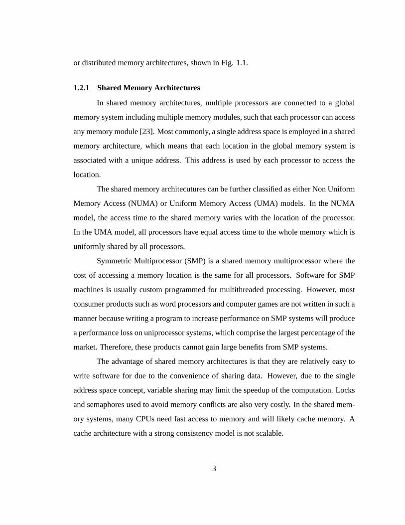
or distributed memory architectures, shown in Fig. 1.1.

1.2.1 Shared Memory Architectures

In shared memory architectures, multiple processors are connected to a global

memory system including multiple memory modules, such thateach processor can access

any memory module [23]. Most commonly, a single address space is employed in a shared

memory architecture, which means that each location in the global memory system is

associated with a unique address. This address is used by each processor to access the

location.

The shared memory architecutures can be further classified as either Non Uniform

Memory Access (NUMA) or Uniform Memory Access (UMA) models.In the NUMA

model, the access time to the shared memory varies with the location of the processor.

In the UMA model, all processors have equal access time to thewhole memory which is

uniformly shared by all processors.

Symmetric Multiprocessor (SMP) is a shared memory multiprocessor where the

cost of accessing a memory location is the same for all processors. Software for SMP

machines is usually custom programmed for multithreaded processing. However, most

consumer products such as word processors and computer games are not written in such a

manner because writing a program to increase performance onSMP systems will produce

a performance loss on uniprocessor systems, which comprisethe largest percentage of the

market. Therefore, these products cannot gain large benefits from SMP systems.

The advantage of shared memory architectures is that they are relatively easy to

write software for due to the convenience of sharing data. However, due to the single

address space concept, variable sharing may limit the speedup of the computation. Locks

and semaphores used to avoid memory conflicts are also very costly. In the shared mem-

ory systems, many CPUs need fast access to memory and will likely cache memory. A

cache architecture with a strong consistency model is not scalable.

3

Global Memory System

Interconnection Network

Cache

1

Cache

2

Cache

N

Processor

1

Processor

2

Processor

N…

…

Global Memory System

Interconnection Network

Cache

1

Cache

2

Cache

N

Processor

1

Processor

2

Processor

N

Cache

1

Cache

2

Cache

N

Processor

1

Processor

2

Processor

N…

…

Interconnection Network

Processor

1

Processor

2

Processor

N

Cache

1

Cache

2

Cache

N…

…

Memory

1

Memory

2

Memory

N…

Interconnection Network

Processor

1

Processor

2

Processor

N

Cache

1

Cache

2

Cache

N…

…

Interconnection Network

Processor

1

Processor

2

Processor

N

Cache

1

Cache

2

Cache

N…

…

Memory

1

Memory

2

Memory

N…Memory

1

Memory

2

Memory

N…

(a) (b)

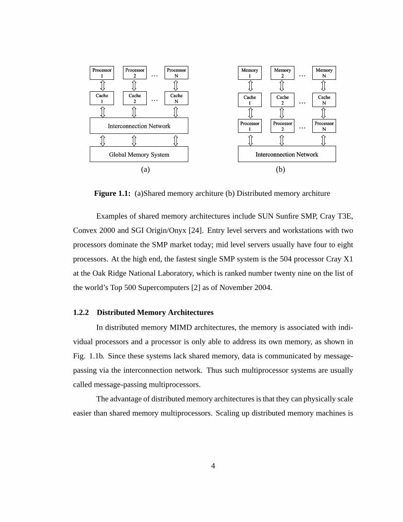
Figure 1.1: (a)Shared memory architure (b) Distributed memory architure

Examples of shared memory architectures include SUN SunfireSMP, Cray T3E,

Convex 2000 and SGI Origin/Onyx [24]. Entry level servers andworkstations with two

processors dominate the SMP market today; mid level serversusually have four to eight

processors. At the high end, the fastest single SMP system isthe 504 processor Cray X1

at the Oak Ridge National Laboratory, which is ranked number twenty nine on the list of

the world’s Top 500 Supercomputers [2] as of November 2004.

1.2.2 Distributed Memory Architectures

In distributed memory MIMD architectures, the memory is associated with indi-

vidual processors and a processor is only able to address itsown memory, as shown in

Fig. 1.1b. Since these systems lack shared memory, data is communicated by message-

passing via the interconnection network. Thus such multiprocessor systems are usually

called message-passing multiprocessors.

The advantage of distributed memory architectures is that they can physically scale

easier than shared memory multiprocessors. Scaling up distributed memory machines is

4

simply adding communication links to connect additional processors to existing proces-

sors. The drawback is that its message-passing mechanism isnot as attractive for pro-

grammers. It usually requires the programmers to provide the explicit message-passing

calls in the code. This may be problematic for applications that require sharing large

amounts of data.

Intel Paragon, CM-5, and Transputers [24] are a few examples of distributed mem-

ory machines. Cluster computing and grid computing are two ofthe most popular exam-

ples.

1.2.2.1 Cluster Computing

A computer cluster is a group of independent computers connected into a unified

system through software and networking [21]. One of the mostpopular implementations

is a cluster-based on commodity hardware, on a private system network, with an open

source software (Linux) infrastructure. This configuration is often referred to as a Be-

owulf cluster [1]. The Beowulf Project was started in early 1994. The initial prototype

was a cluster computer consisting of 16 DX4 processors connected by a channel bonded

Ethernet. The top supercomputer as of November 2004 is the Department of Energy’s

BlueGene/L cluster system [25].

There are several factors that have contributed to the success of the Beowulf cluster

project. First of all, market competition has driven the prices down and reliability up for

the subsystems, including microprocessors, motherboards, disks and network systems.

Secondly, open source software, particularly the Linux operating system, GNU compilers,

programming tools, MPI and PVM message-passing libraries are now available. Thirdly,

an increased reliance on computational science demands high performance computing.

Typical applications include bioinformatics, financial market modelling, data mining, and

Internet servers for audio and games.

PVM (Parallel Virtual Machine) [26] and MPI (Message Passing Interface) [27]

are software packages for parallel programming on a cluster. PVM used to be the standard

5

until MPI appeared. PVM was developed by the University of Tennessee, the Oak Ridge

National Laboratory and Emory University. The first versionwas written at ORNL in

1989. MPI is the standard for portable message-passing parallel programs. It is a library

of routines that can be called from Fortran, C and C++ programs. MPI’s advantage over

older message-passing libraries is that it is both portableand fast.

1.2.2.2 Grid Computing

CERN (an European Organization for Nuclear Research), which was a key in the

creation of the World Wide Web, defines the “Grid” as: “a service for sharing computer

power and data storage capacity over the Internet” [21]. Grid computing offers a model for

solving massive computational problems by making use of theunused resources of large

numbers of computers treated as a virtual cluster embedded in a distributed telecommu-

nications infrastructure.

Grid computing has the following features: (1), It allows the virtualization of

disparate IT resources. (2), It allows the sharing of resources, which include not only files

but also computing power. (3), It is often geographically distributed and heterogeneous,

which makes it different from cluster computing.

Typical applications of grid computing include grand challenging problems like

protein folding, financial modeling, earthquake simulation, climate/weather modelling

etc. An example of grid computing is BIRN (Biomedical Informatics Research Net-

work), which is a National Institutes of Health initiative providing an information tech-

nology infrastructure, notably a grid of supercomputers, for distributed collaborations in

biomedical science.

1.2.3 Multithreaded Architectures

The design concept of computer architecture over the last two decades has been

mainly on the exploitation of the instruction level parallelism, such as pipelining, VLIW

6

(Very Long Instruction Word) or superscalar architecture [24]. Pipelining is now uni-

versally implemented in high-performance processors. Superscalar means the ability to

fetch, issue to execution units, and complete more than one instruction at a time. Similar

to superscalar architectures, VLIW enables the CPU to execute several instructions at the

same time and uses software to decide which operations can run in parallel. Superscalar

CPUs, in contrast, use hardware to decide which operations can run in parallel.

However, the major processor manufactures have run out of room with the tra-

ditional approaches to boosting CPU performance, such as increasing clock frequency,

execution optimization (pipelining, branch prediction, VLIW and superscalar), as well as

increasing the size of cache [9]. First of all, as the clock frequency increases, the transis-

tor leakage current also increases, leading to excessive power consumption. Second, the

design concepts of traditional approaches have become too complex. Third, resistance

capacitance delays in signal transmission grow as feature sizes shrink, imposing an addi-

tional bottleneck that frequency increases do not address.Also, for certain applications,

traditional serial architectures are becoming less efficient as processors get faster due to

the effect of the Von Neuman bottleneck [28].

In addition, the advantages of higher clock speeds are negated by memory latency.

There are many commercial or scientific applications which have frequent memory ac-

cess, and the performance of such applications is dominatedby the cost of memory ac-

cess. As pointed out in many papers, microprocessor performance has been doubling

every 18-24 months for many years, while DRAM performance only improves by 7% per

year [29]. Therefore the memory access latency continues togrow in terms of CPU cy-

cles. The divergence of the CPU and memory speed is generally referred to as the “mem-

ory wall” problem. Assuming 20% of the total instructions ina program need to access

memory, which means, one of every five instructions during execution accesses memory,

the system will hit the memory wall if the average memory access time is greater than 5

instruction cycles [30].

7

Therefore, for the next generation of computer architectures, multithreaded archi-

tectures are becoming more popular. Depending on the specific form of a multithreaded

processor, a thread could be a full program (single-threaded UNIX process), an operating

system thread (a light-weighted process, e.g., a POSIX thread [31]), a compiler-generated

thread, or a hardware generated thread [5].

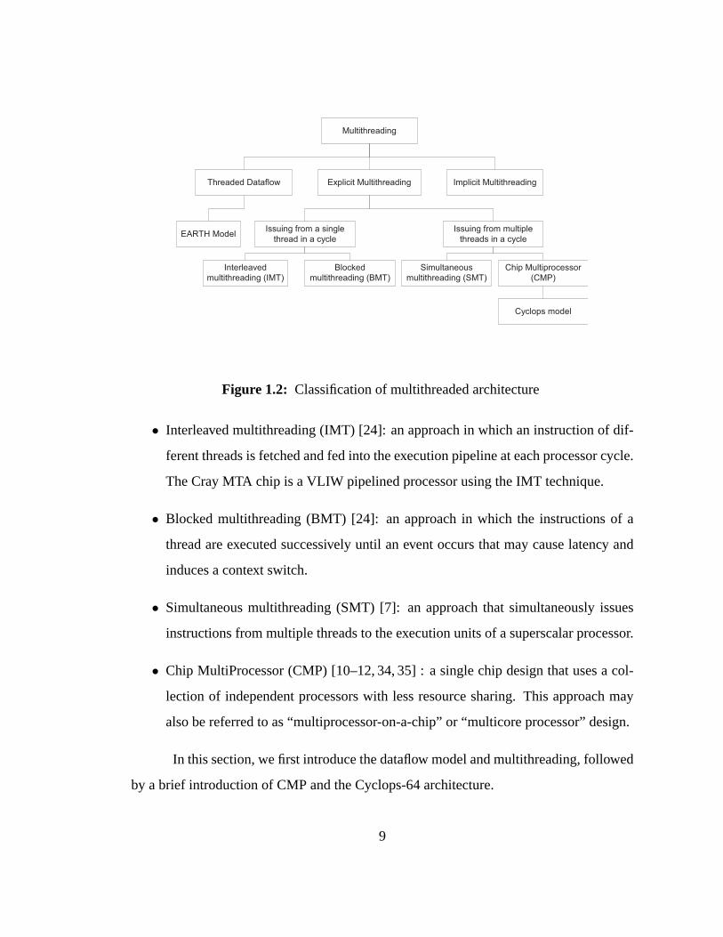
1.2.3.1 Classification

Multithreaded models can be classified according to the thread scheduling mecha-

nisms (preemptive or non-preemptive), architectural features and memory models (shared

memory or distributed memory), or program flow mechanisms (dataflow or control flow)

[32].

According to the classification in [5], multithreaded architectures in the more nar-

row sense only include architectures that stem from the modification of scalar RISC,

VLIW, or superscalar processors. The classification from [5] is shown in Fig. 1.2. The

terminologies in the figure are explained as follows:

• Threaded dataflow [33]: a combination of multithreading andthe dataflow model.

This model uses the dataflow principle to start the executionof a non-preemptive

thread.

• Explicit multithreading [5]: an approach that explicitly executes instructions of

different user-defined threads (operating system threads or processes) in the same

pipeline.

• Implicit multithreading [5]: an approach that adopts thread level speculation, dy-

namically generates speculative threads from single-threaded programs and exe-

cutes them concurrently with the lead thread.

8

Multithreading

Threaded Dataflow Explicit Multithreading Implicit Multithreading

Issuing from a single

thread in a cycle

Issuing from multiple

threads in a cycleEARTH Model

Interleaved

multithreading (IMT)

Blocked

multithreading (BMT)

Simultaneous

multithreading (SMT)

Chip Multiprocessor

(CMP)

Cyclops model

Figure 1.2: Classification of multithreaded architecture

• Interleaved multithreading (IMT) [24]: an approach in which an instruction of dif-

ferent threads is fetched and fed into the execution pipeline at each processor cycle.

The Cray MTA chip is a VLIW pipelined processor using the IMT technique.

• Blocked multithreading (BMT) [24]: an approach in which the instructions of a

thread are executed successively until an event occurs thatmay cause latency and

induces a context switch.

• Simultaneous multithreading (SMT) [7]: an approach that simultaneously issues

instructions from multiple threads to the execution units of a superscalar processor.

• Chip MultiProcessor (CMP) [10–12, 34, 35] : a single chip design that uses a col-

lection of independent processors with less resource sharing. This approach may

also be referred to as “multiprocessor-on-a-chip” or “multicore processor” design.

In this section, we first introduce the dataflow model and multithreading, followed

by a brief introduction of CMP and the Cyclops-64 architecture.

9

1.2.3.2 Data Flow Multithreading

The dataflow model [6, 36] is a dramatic break from the traditional von Neumann

model [37]. In the von Neumann computer, a single program counter determines which

instruction to execute next and a complete order exists between instructions. The dataflow

model, in contrast, only has apartial order between instructions. The fundamental idea

of dataflow is that any instruction can be executed as long as its operands are present.

The combination of the von Neumann model and the dataflow model [38] puts two

or more dataflow actors into threads; therefore, it can reduce fine-grain synchronization

costs and improve locality in dataflow architectures. It canalso add latency-tolerance and

efficient synchronization to conventional multithreaded machines by integrating dataflow

synchronization into the thread model.

According to Dennis and Gao [33], a thread is viewed as a sequentially ordered

block of instructions with a grain-size greater than one. Evaluation of a non-preemptive

thread starts as soon as all input operands are available, adopting the idea of the dataflow

model. Access to remote data is organized in a split-phase manner by one thread sending

the access request to memory and another thread activating when its data is available.

Thus a program is compiled into many, very small threads activating each other when

data become available.

EARTH (Efficient Architecture for Running THreads) [3, 4] is one example of the

multithreaded data flow model. More details of the EARTH model are presented in next

chapter. The EARTH model is currently supported on both SMP machines and cluster

computers.

1.2.3.3 Multiprocessor-on-a-Chip Model

The “multiprocessor-on-a-chip” model is a single chip design that uses a collec-

tion of independent processors with less resource sharing.Currently available multicore

processors include IBM’s dual-core Power4 and Power5, Hewlett-Packard’s PA-8800 and

10

Sun’s dual-core Sparc IV. AMD will deliver dual-core Opterons around the middle of

2005. Intel also makes shifts to multicore chips this year.

Intel researchers and scientists are experimenting with many tens of cores, poten-

tially even hundreds of cores per die. And those cores will support tens, hundreds, maybe

even thousands of simultaneous threads [39]. Intel’s Platform 2015 [28] describes the

evolution of its multiprocessor architecture over the next10 years. Multicore architec-

tures of Platform 2015 and sooner will enable dramatic performance scaling and address

important power management and heat challenges. They will be able to activate only

the cores needed for a given function and power down the idle cores. The features of

the hypothetical Micro 2015 include: (1), Parallelism willbe handled by an abundant

number of software and hardware threads. (2), A relatively large high speed, reconfig-

urable onchip memory will be shared by groups of cores, the OS, the micro kernel and

the special-purpose hardware. (3), Tera-flops of supercomputer-like performance and new

capabilities for new applications and workloads will be provided.

Another representative “multiprocessor-on-a-chip” architecture design is Cyclops-

64 [10–12, 34, 35], a new architecture for high performance parallel computers being de-

veloped at the IBM T. J. Watson Research Center and the University of Delaware. The

basic cell of this architecture is a single chip with multiple threads of execution, embedded

memory, and integrated communication hardware. The memorylatency is tolerated by

the massive intra-chip parallelism. More details of Cyclops-64 architecture are described

in Section 3.2.

11

1.3 Bioinformatics

1.3.1 Definition

Bioinformatics or computational biology is the applicationof computational tools

and techniques to the management and analysis of biologicaldata [40]. It is a rapidly

evolving discipline and involves techniques from applied mathematics, statistics, and

computer science. The terms “bioinformatics” and “computational biology” are often

used interchangeably, although the latter typically focuses on algorithm development and

specific computational methods.

We view bioinformatics research as an integration of biological data management

and knowledge discovery. Biological data management enables efficient storage, orga-

nization, retrieving, and sharing of different types of information. Knowledge discovery

involves the development of new algorithms to analyze and interpret various types of data,

as well as the development and implementation of software tools.

Bioinformatics has many practical applications in different areas of biology and

medicine. More specifically, major research efforts in the field include sequence align-

ment, gene finding, genome assembly, protein structure alignment and prediction, and the

modeling of evolution.

1.3.2 Role of High Performance Computing

Bioinformatics has inspired computer science advances withnew concepts, new

ideas and new designs. In turn, the advances in computer hardware and software algo-

rithms have also revolutionized the area of bioinformatics. The cross-fertilization has

benefited both fields and will continue to do so. The role of high performance comput-

ing in bioinformatics can be reflected from two angles: (1) large amounts of data; (2)

computationally challenging problems.

Firstly, large amounts of data create an urgent need for highperformance comput-

ing. For example, the genetic sequence information in the National Center for Biotech-

nology GenBank (NCBI) database [41] has more than 44 billion base pairs as of April

12

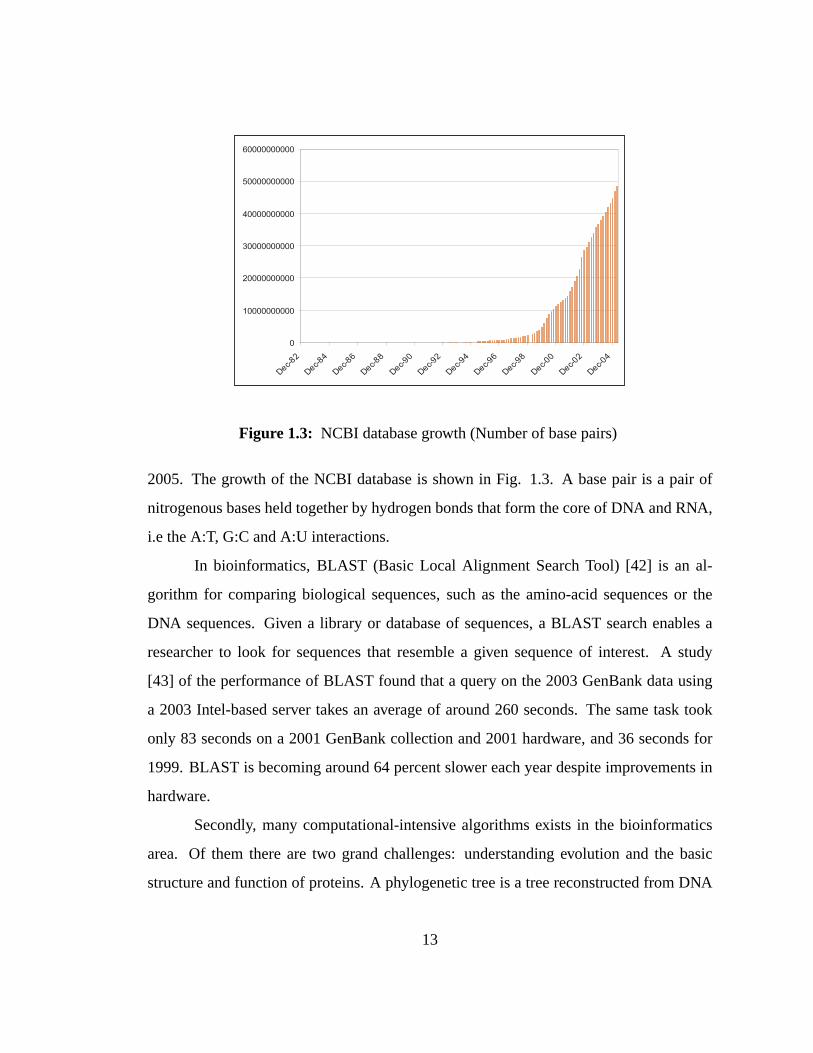
0

10000000000

20000000000

30000000000

40000000000

50000000000

60000000000

Dec-

82

Dec-

84

Dec-

86

Dec-

88

Dec-

90

Dec-

92

Dec-

94

Dec-

96

Dec-

98

Dec-

00

Dec-

02

Dec-

04

Figure 1.3: NCBI database growth (Number of base pairs)

2005. The growth of the NCBI database is shown in Fig. 1.3. A basepair is a pair of

nitrogenous bases held together by hydrogen bonds that formthe core of DNA and RNA,

i.e the A:T, G:C and A:U interactions.

In bioinformatics, BLAST (Basic Local Alignment Search Tool)[42] is an al-

gorithm for comparing biological sequences, such as the amino-acid sequences or the

DNA sequences. Given a library or database of sequences, a BLAST search enables a

researcher to look for sequences that resemble a given sequence of interest. A study

[43] of the performance of BLAST found that a query on the 2003 GenBank data using

a 2003 Intel-based server takes an average of around 260 seconds. The same task took

only 83 seconds on a 2001 GenBank collection and 2001 hardware, and 36 seconds for

1999. BLAST is becoming around 64 percent slower each year despite improvements in

hardware.

Secondly, many computational-intensive algorithms exists in the bioinformatics

area. Of them there are two grand challenges: understandingevolution and the basic

structure and function of proteins. A phylogenetic tree is atree reconstructed from DNA

13

or protein sequences to represent the history of evolution.Phylogenetic tree reconstruc-

tions involve solving difficult optimization problems witha complexity of(2n − 5)!! for

a tree withn leafs and requires months to years of computation. Many approaches have

been proposed to reconstruct phylogenetic tree using the power of high performance com-

puting, such as parallel fast DNAml [44] and GRAPPA [16, 45]. These approaches still

have limitations such as tree size and accuracy. The proteinfolding simulation is a popular

way to predict the structure and function of proteins. Protein folding refers to a process by

which a protein assumes its three-dimensional shape with which they are able to perform

their biological function. According to an estimate [46], accurate simulation of a protein

folding to predict the protein 3D structure may be intractable without PetaFLOPS-class

computers. Simulating 100 microseconds of protein foldingwould take three years on

even a PetaFLOPS system or keep a 3.2GHz microprocessor busyfor the next million

centuries. Therefore, new approaches of high performance computing and algorithmic

design need to be developed to meet these challenges.

14

1.4 Achievements and Contributions

The principal goal of this research is to find better solutions for important and

practical bioinformatics or biomedical applications. Thecontribution of our work is two-

fold. On the one hand, we parallelize and optimize the real, large scale applications,

dramatically decreasing the time for computation. On the other hand, we experimental

results of the applications provide new insights for the design of computer architectures.

The applications include the Hmmpfam database search program from the bioin-

formatics area, the SPACE RIP image reconstruction from the biomedical area, and an-

other very useful biomedical application – using halftoning algorithms to make graphics

available to people with visual impairment. These three applications fall into the gen-

eral umbrella of bio-oriented applications. The first two applications are closely related

to parallel computing; the last application, in contrast, is not as closely related. This is,

however, a natural result of the multi-disciplinary characteristic of this research.

Hmmpfam is a widely-used computation-intensive bioinformatics software for se-

quence classification. Sequence classification plays an important role in bioinformatics to

predict the protein structure and function. The major achievements are listed as follows:

1. We analyzed the Hmmpfam program structure and proposed a new task decompo-

sition scheme to reduce data communication and improve program scalability.

2. We implemented a scalable and robust cluster-based parallel Hmmpfam using

EARTH (Efficient Architecture for Running Threads), an event-driven fine-grain

multithreaded programming execution model.

3. Our new parallel scheme and implementation achieved notable improvements in

terms of program scalability. We conducted experiments on two advanced super-

computing clusters at the Argonne National Laboratory (ANL) and achieved an

absolute speedup of 222.8 on 128 dual-CPU nodes for a representative data set.

15

The application SPACE RIP (Sensitivity Profiles From an Array of Coils for En-

coding and Reconstruction in Parallel) is one of the parallelimaging methods that has the

potential to revolutionize the field of fast MR imaging. The image reconstruction prob-

lem of SPACE RIP is a computation-intensive task, and thus a potential application for

parallel computing. The major contributions of our work aresummarized as follows:

1. We implemented the parallelization and optimization of SPACE RIP at three lev-

els. The top level is the loop level parallelization, which decomposes SPACE RIP

into many tasks of a singular value decomposition (SVD) problem. The middle

level parallelizes the SVD problem using the one-sided Jacobi algorithm and is

implemented on Cyclops-64. At this level, an SVD problem is decomposed into

many matrix column rotation routines. The bottom level further optimizes the ma-

trix column rotation routine using several memory preloading or loop unrolling

approaches.

2. We developed a model and trace analyzer to decompose the total execution cycles

into four parts: total instruction counts, “DLL”, “DLF” and“DLI”, where “DLL”

represents the cycles spent on memory access, “DLF” represents the latency cy-

cles related to floating point operations, and “DLI” represents the latency cycles

related to integer operations. This simple model allows us to study the application

performance tradeoff for different algorithms.

3. Using a few application parameters such as matrix size, group size, and architec-

tural parameters such as onchip and offchip latency, we developed analytical equa-

tions for comparing different memory access approaches such as preloading and

loop unrolling. We used a cycle accurate simulator to validate the analysis and

compare the effect of different approaches on the “DLL” partand total execution

cycles.

16

The application of using halftoning to generate tactile graphics uses signal

processing algorithms and computer technologies to aid blind people. Tactile imaging

is an algorithmic process that converts a visual image into an image perceivable by the

sense of touch. Tactile imaging translates a visual image into an image perceivable by the

sense of touch. Digital halftoning creates the illusion of acontinuous-tone image from the

judicious arrangement of binary picture elements. As an extension of binary halftoning,

multilevel halftoning techniques are adopted on printers that can generate multiple output

levels. We exploited the TIGER (Tactile Graphics Embosser)printer’s variable-height

punching ability to convert graphics to multilevel halftoning tactile texture patterns. The

major contributions are summarized as follows:

1. We introduced digital halftoning into the field of tactileimaging and implemented

four different halftoning algorithms into the TIGER printer driver.

2. According to the specifics of the TIGER printer, we extended traditional binary

halftoning algorithms to multilevel algorithms.

3. We conducted experiments to compare the halftoning-based approach with the

simple, commonly utilized thresholding-based approach and observed that the

halftoning-based approach achieved significant improvement in terms of its texture

pattern discrimination ability.

1.5 Publications

This dissertation is based on several published works. The work on the parallel

Hmmpfam is published in Cluster2003 and the International Journal of High Performance

Computing and Networking (IJHPCN) [47]. The work on SPACE RIP andSVD is in-

cluded in the proceedings of the 16th IASTED International Conference on Parallel and

Distributed Computing and Systems [48]. The work on tactile graphics using halfton-

ing is summarized in a paper submitted to the IEEE Transactions on Neural Systems and

Rehabilitation Engineering [49].

17

1.6 Dissertation Organization

The remainder of this dissertation is organized as follows.Chapters 2, 4 and 3 fo-

cus on the applications Parallel Hmmpfam, tactile graphics, parallel SPACE RIP respec-

tively. Chapter 2 includes background information about theHidden Markov Model and

its application in the bioinformatics area, an introduction of the Hmmpfam program, the

original parallel scheme in the PVM implementation, the proposed cluster-based parallel

implementation and the performance results. Chapter 3 presents the background infor-

mation of Cyclops-64, the parallel imaging technique SPACE RIP, the loop level and fine

level parallel scheme, a performance model for different memory access schemes, and

the performance results. Chapter 4 includes a brief review oftactile printing, the TIGER

printer hardware and software, a discussion on the basics ofhalftoning techniques, and the

implementation of the halftoning algorithm into the TIGER printer graphics processing

pipeline, as well as the experimental design and evaluationresults. Chapter 5 concludes

this dissertation.

18

Chapter 2

A CLUSTER-BASED SOLUTION FOR HMMPFAM

2.1 Introduction

One of the fundamental problems in computational biology isthe classification of

proteins into functional and structural classes or families based on homology of protein

sequence data. Sequence database searching and family classification are common ways

to analyze the function and structure of the sequences. A “family” is a group of proteins of

similar biochemical function that are more than 50% identical [50]. Sequence homology

indicates a common function and common ancestry of two DNA orprotein sequences.

The family classification of sequences is of particular interest to drug discovery

research. For example, if an unknown sequence is identified as belonging to a certain

protein family, then its structure and function can be inferred from the information of that

family. Furthermore if this sequence is sampled from certain diseases X and belongs to a

family F, then X can be treated using the combination of existing drugs for F [51].

Typical approaches for protein classification include pairwise sequence alignment

[13, 42], consensus patterns using motifs [52] and profile hidden Markov models (profile

HMMs) [53–55]. A profile HMM is a consensus HMM model built from a multiple

sequence alignment of protein families. HMM is a probabilistic graphical model used

very widely in speech recognition and other areas [56]. In recent years, HMM has been an

important research topic in the bioinformatics area. It is applied systematically to model,

align, and analyze entire protein families and the secondary structure of sequences. A

consensus sequence of a family can be determined by derivingthe profile HMM. Unlike

19

P(H|S1)=0.5

P(T|S1)=0.5

S1

P(H|S2)=0.7

P(T|S2)=0.3

S2

0.9

0.1

0.1

0.9

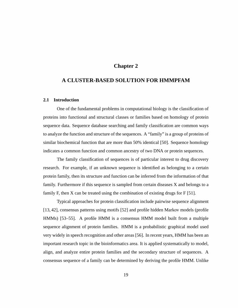
Figure 2.1: HMM model for tossing coins

conventional pairwise comparisons, a consensus model can in principle exploit additional

information such as the position and identity of residues that are more or less conserved

throughout the family, as well as variable insertion and deletion probabilities [57].

A very simple example of HMM for tossing coins is given in Fig.2.1. We use a

fair coin or a biased coin which has a probability of 0.7 to geta “head”. We change coins

with a probability of 0.1. The corresponding HMM is:

• The states areQ = {S1, S2}, whereS1 stands for “fair” andS2 for “biased”.

• Transition probabilities are:α11 = 0.9, α12 = 0.1, α21 = 0.1, α22 = 0.9.

• Emission probabilities are:P (H|S1) = 0.5, P (T |S1) = 0.5, P (H|S2) = 0.7,

P (T |S2) = 0.3.

In this example, the observation is “Head” or “Tail”. The statesS1 andS2 are not observ-

able, thus the name “hidden”. Assuming thatS1 is the initial state, we can compute the

probability of observing a certain sequence. For example:

P (HH|M) = P (H|S1) × 0.9 × P (H|S1) + P (H|S1) × 0.1 × P (H|S2) (2.1)

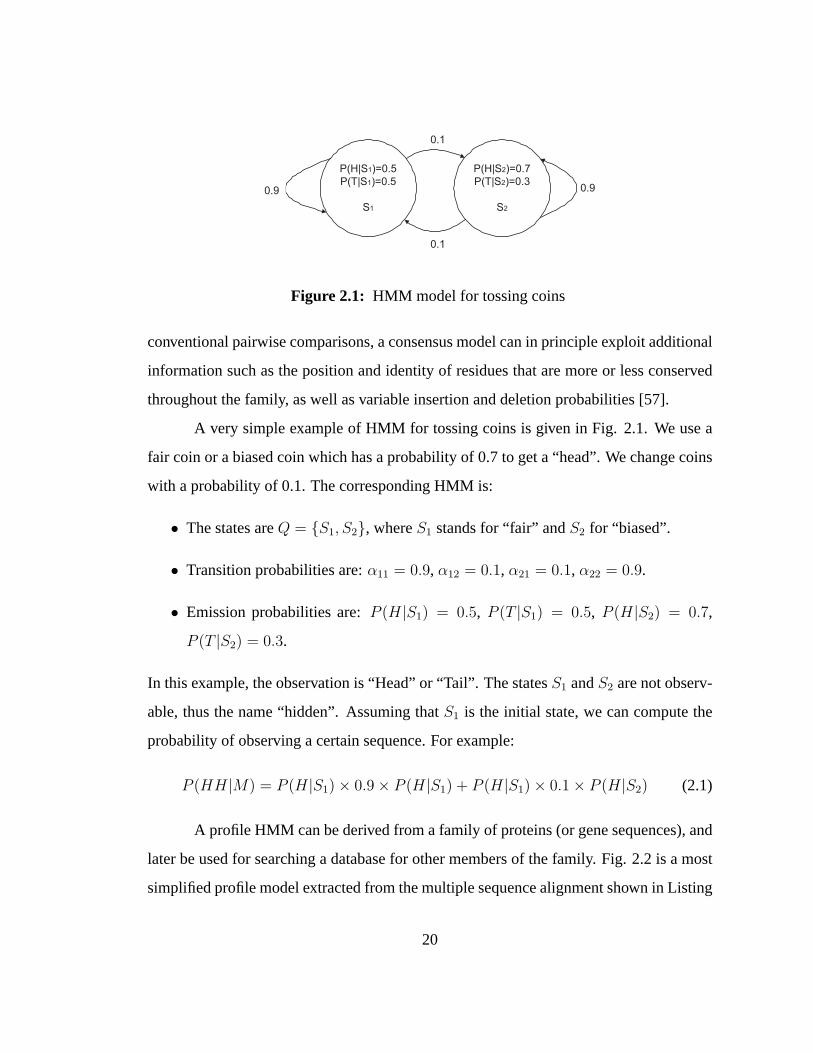
A profile HMM can be derived from a family of proteins (or gene sequences), and

later be used for searching a database for other members of the family. Fig. 2.2 is a most

simplified profile model extracted from the multiple sequence alignment shown in Listing

20

2.1. Each block in the figure corresponds to one column in the multiple sequence align-

ment. The emission probabilities are listed in each block, and the transition probabilities

are shown on the black arrows. The detailed process of initialization of an HMM from a

multiple sequence alignment is reviewed in [57].

seq1 : C A − − − A Tseq2 : C A A C T A Tseq3 : G A C− − A Gseq4 : G A − − − A Tseq5 : C C G− − A T

Listing 2.1: DNA sequence alignment

There are three types of questions related to profile HMM [57]: (1) How do we

build an HMM to represent a family? (2) Does a sequence belongto a family? For a

given sequence, what is the probability that this sequence has been produced by an HMM

model? (3) Assuming that the transition and emission parameters are not known with

certainty, how should their values be revised in light of theobserved sequence? The

problem solved in this research falls into the second category.

Usually, for a given unknown sequence, it is necessary to do adatabase search

against an HMM profile database which contains several thousands of families. HMMER

[14] is an implementation of profile HMMs for sensitive database searches. A wide col-

lection of protein domain models have been generated by using the HMMER package.

These models have largely comprised the Pfam protein familydatabase [58–60].

Pfam (Protein families database of alignments and HMMs) is adatabase of protein

domain families. A “domain” in the sequence context is an extended sequence pattern

that indicates a common evolutionary origin. It also refersto a segment of a polypeptide

chain that folds into a three-dimensional structure [50] inthe “structural” context. The

Pfam database contains multiple sequence alignments for each family, as well as profile

HMMs for finding these domains in new sequences. Each Pfam family has two multiple

21

A 0.0

C 0.6

G 0.4

T 0.0

A 0.8

C 0.2

G 0.0

T 0.0

A 1.0

C 0.0

G 0.0

T 0.0

A 0.0

C 0.0

G 0.2

T 0.8

1.0 0.4 1.0

A 0.2

C 0.4

G 0.2

T 0.2

0.4

0.6 0.6

Figure 2.2: HMM model for a DNA sequence alignment

alignments: the seed alignment that contains a relatively small number of representative

members of the family and the full alignment that contains all members. In the past 2

years, Pfam has split many existing families into structural domains. Currently, in the

Pfam database, one-third of entries contain at least one protein of known 3D structure.

Pfam also contains functional annotation, literature references and database links for each

family.

Hmmpfam, one program in the HMMER 2.2g package, is a tool for searching a

single sequence against an HMM database. In real situations, this program may take a

few weeks to a few months to process large amounts of sequencedata. Thus efficient

parallelization of the Hmmpfam is essential to bioinformatics research.

HMMER 2.2g provides a parallel Hmmpfam program based on PVM (Parallel

Virtual Machine) [26]. However, the PVM version does not have good scalability and

cannot fully take advantage of the current advanced supercomputing clusters. So a highly

scalable and robust cluster-based solution for Hmmpfam is necessary. We implemented

a parallel Hmmpfam harnessing the power of a multithreaded architecture and program

execution model – the EARTH (Efficient Architecture for Running THreads) model [3, 4],

where parallelism can be efficiently exploited on top of a supercomputing cluster built

22

with off-the-shelf microprocessors.

The major contributions of this research are as follows: (1)the first EARTH-

based parallel implementation of a bioinformatics sequence classification application; (2)

a largely scalable parallel Hmmpfam implementation targeted to advanced supercomput-

ing clusters; (3) the implementation of a new efficient master-slave dynamic load balancer

in the EARTH runtime system. This load balancer is targeted to parallel applications

adopting a master-slave model and shows more robust performance than a static load

balancer.

The remainder of this chapter is organized as follows. In section 2.2, we review the

Hmmpfam program and the original parallel scheme implemented on PVM, the EARTH

model is reviewed in 2.3. Our cluster-based multithreaded parallel implementation is

described in section 2.4 and section 2.5. The performance results of our implementation

are presented in section 2.6, and conclusions in section 2.7.

2.2 HMMPFAM Algorithm and PVM Implementation

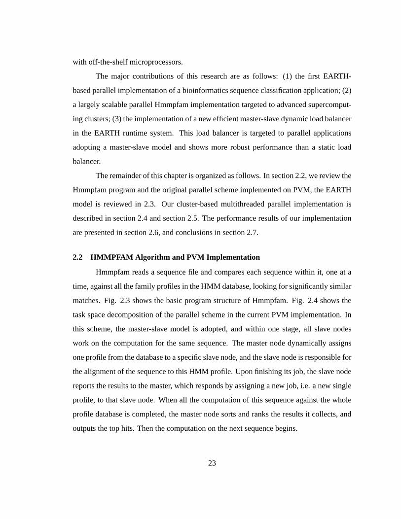
Hmmpfam reads a sequence file and compares each sequence within it, one at a

time, against all the family profiles in the HMM database, looking for significantly similar

matches. Fig. 2.3 shows the basic program structure of Hmmpfam. Fig. 2.4 shows the

task space decomposition of the parallel scheme in the current PVM implementation. In

this scheme, the master-slave model is adopted, and within one stage, all slave nodes

work on the computation for the same sequence. The master node dynamically assigns

one profile from the database to a specific slave node, and the slave node is responsible for

the alignment of the sequence to this HMM profile. Upon finishing its job, the slave node

reports the results to the master, which responds by assigning a new job, i.e. a new single

profile, to that slave node. When all the computation of this sequence against the whole

profile database is completed, the master node sorts and ranks the results it collects, and

outputs the top hits. Then the computation on the next sequence begins.

23

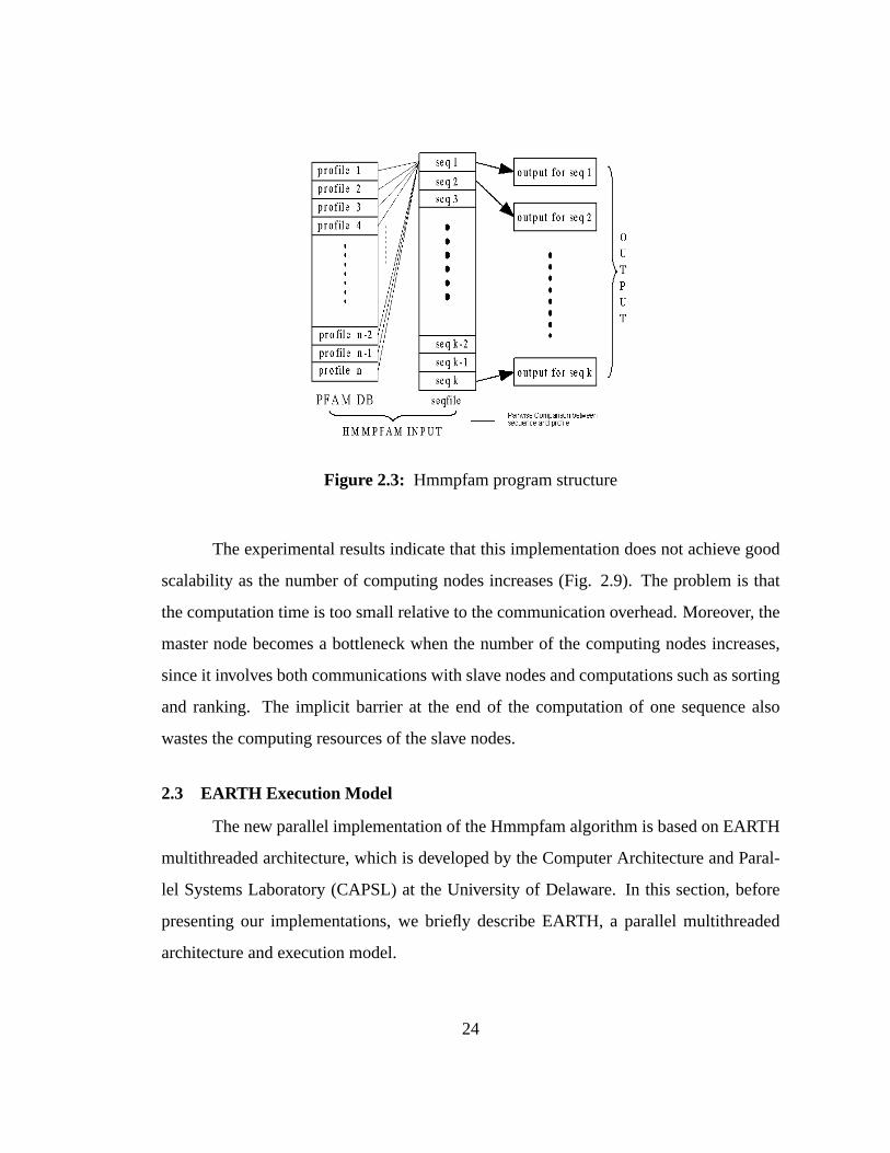
Figure 2.3: Hmmpfam program structure

The experimental results indicate that this implementation does not achieve good

scalability as the number of computing nodes increases (Fig. 2.9). The problem is that

the computation time is too small relative to the communication overhead. Moreover, the

master node becomes a bottleneck when the number of the computing nodes increases,

since it involves both communications with slave nodes and computations such as sorting

and ranking. The implicit barrier at the end of the computation of one sequence also

wastes the computing resources of the slave nodes.

2.3 EARTH Execution Model

The new parallel implementation of the Hmmpfam algorithm isbased on EARTH

multithreaded architecture, which is developed by the Computer Architecture and Paral-

lel Systems Laboratory (CAPSL) at the University of Delaware. In this section, before

presenting our implementations, we briefly describe EARTH,a parallel multithreaded

architecture and execution model.

24

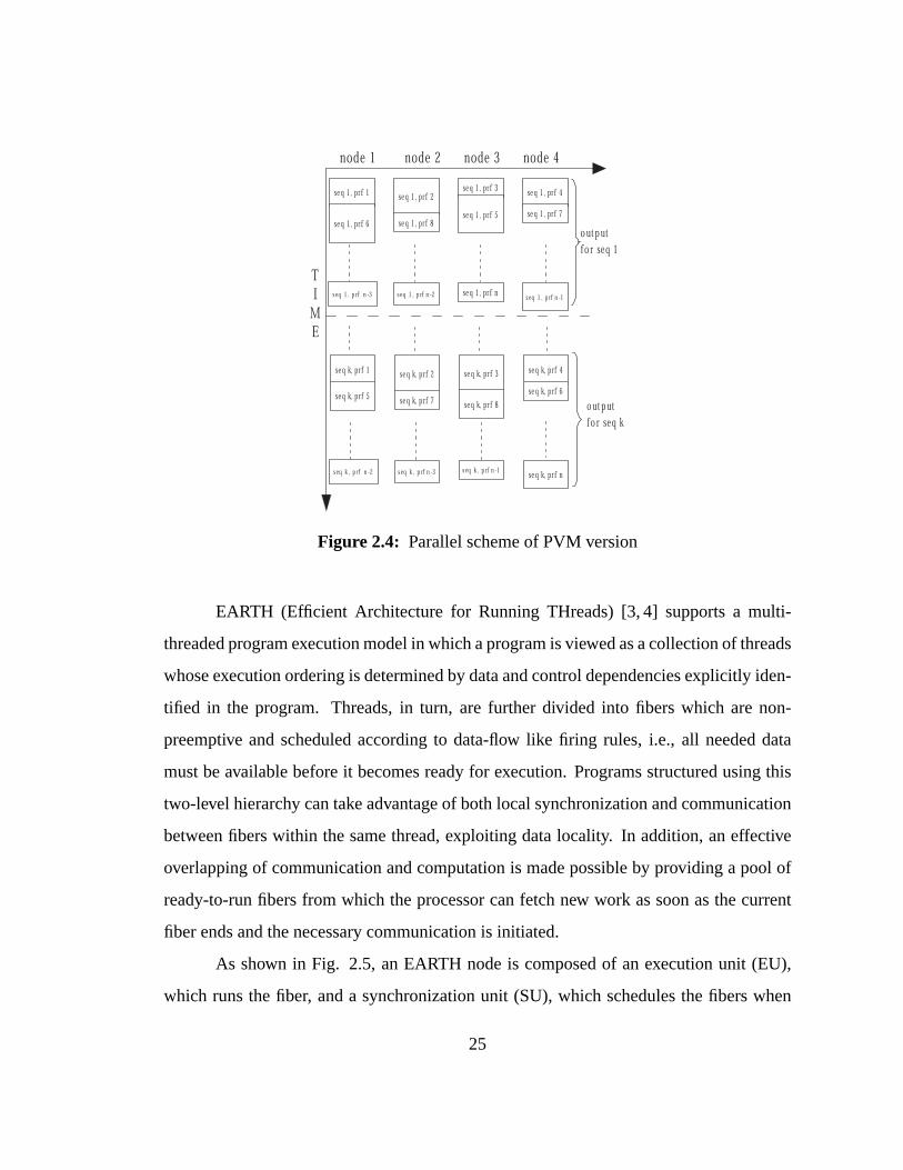
TI

ME

node 1 node 3node 2 node 4

se q 1, prf 1 se q 1, prf 2se q 1, prf 3

se q 1, prf 4

se q 1, prf 5se q 1, prf 6

se q 1, prf 7se q 1, prf 8

seq 1 , p rf n -3 seq 1 , p rf n -2 se q 1, prf nseq 1 , p rf n -1

o ut p ut

fo r seq 1

se q k, prf 1 se q k, prf 2 se q k, prf 3 se q k, prf 4

se q k, prf 8se q k, prf 5

se q k, prf 6se q k, prf 7

seq k , p rf n -2 seq k , p rf n -3 seq k , p rf n -1se q k, prf n

o ut p ut

fo r seq k

Figure 2.4: Parallel scheme of PVM version

EARTH (Efficient Architecture for Running THreads) [3, 4] supports a multi-

threaded program execution model in which a program is viewed as a collection of threads

whose execution ordering is determined by data and control dependencies explicitly iden-

tified in the program. Threads, in turn, are further divided into fibers which are non-

preemptive and scheduled according to data-flow like firing rules, i.e., all needed data

must be available before it becomes ready for execution. Programs structured using this

two-level hierarchy can take advantage of both local synchronization and communication

between fibers within the same thread, exploiting data locality. In addition, an effective

overlapping of communication and computation is made possible by providing a pool of

ready-to-run fibers from which the processor can fetch new work as soon as the current

fiber ends and the necessary communication is initiated.

As shown in Fig. 2.5, an EARTH node is composed of an executionunit (EU),

which runs the fiber, and a synchronization unit (SU), which schedules the fibers when

25

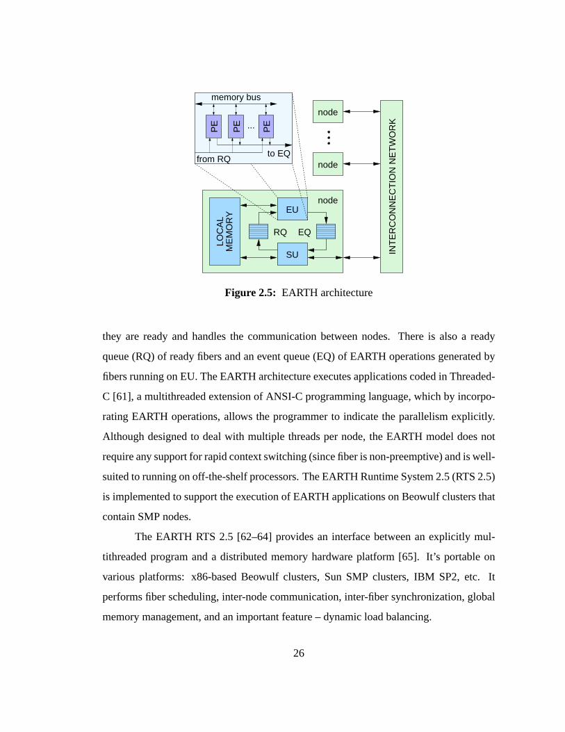
INT

ER

CO

NN

EC

TIO

N N

ET

WO

RK

LOC

AL

ME

MO

RY

SU

EUnode

EQ

node

node

...PE

PE

PE

RQ

from RQto EQ

memory bus

Figure 2.5: EARTH architecture

they are ready and handles the communication between nodes.There is also a ready

queue (RQ) of ready fibers and an event queue (EQ) of EARTH operations generated by

fibers running on EU. The EARTH architecture executes applications coded in Threaded-

C [61], a multithreaded extension of ANSI-C programming language, which by incorpo-

rating EARTH operations, allows the programmer to indicatethe parallelism explicitly.

Although designed to deal with multiple threads per node, the EARTH model does not

require any support for rapid context switching (since fiberis non-preemptive) and is well-

suited to running on off-the-shelf processors. The EARTH Runtime System 2.5 (RTS 2.5)

is implemented to support the execution of EARTH applications on Beowulf clusters that

contain SMP nodes.

The EARTH RTS 2.5 [62–64] provides an interface between an explicitly mul-

tithreaded program and a distributed memory hardware platform [65]. It’s portable on

various platforms: x86-based Beowulf clusters, Sun SMP clusters, IBM SP2, etc. It

performs fiber scheduling, inter-node communication, inter-fiber synchronization, global

memory management, and an important feature – dynamic load balancing.

26

2.4 New Parallel Scheme

2.4.1 Task Decomposition

To efficiently parallelize an application, it is important to determine a proper task

decomposition scheme. In parallel computing, we normally decompose a problem into

many small tasks that run in parallel. A smaller task size means that relatively small

amounts of computational work are done between communication events, which, in turn,

implies a low computation-to-communication ratio and highcommunication overhead.

A smaller task size, however, facilitates load balancing. We often use “granularity” as

a qualitative measure of the ratio of computation-to-communication. Finer granularity

means a smaller task size. The proper granularity depends onthe algorithm and the

hardware environment.

In the original scheme, the alignment of one sequence with one profile is treated

as a single task. In order to reduce communication overhead,our scheme considers the

computation of one sequence against the whole database as a single task. Normally the

number of sequences in a sequence data file is much larger thanthe number of computing

nodes available in current Beowulf clusters. So the number ofsingle tasks is still relatively

large to keep all nodes busy. Usually, the sequences are of similar length; thus we can

also achieve good load balancing even with a bigger task size. Moreover, because the

computation of one single sequence is performed by one process on one fixed node, the

sorting and ranking can be done locally on that particular node, thus freeing the master

from the burden of such computation.

2.4.2 Mapping to the EARTH Model

The EARTH model allows dynamic and hierarchical generationof threaded pro-

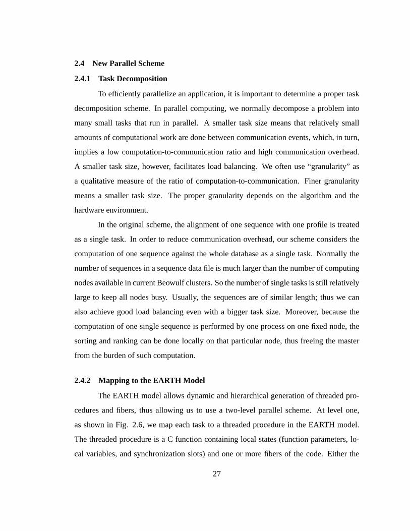
cedures and fibers, thus allowing us to use a two-level parallel scheme. At level one,

as shown in Fig. 2.6, we map each task to a threaded procedure in the EARTH model.

The threaded procedure is a C function containing local states (function parameters, lo-

cal variables, and synchronization slots) and one or more fibers of the code. Either the

27

MA STER

seq 1 vs DB seq 2 vs DB seq k vs DB

seq1 vspart 1 of

DB

seq 1 vspart 2 of

DB

seq 1 vspart mof DB

seq k vspart 1 of

DB

seq k vspart 2 of

DB

seq k vspart mof DB

L e v e l 1

L e v e l 2

Figure 2.6: Two level parallel scheme

programmer or EARTH RTS can determine where (on which node) aprocedure gets

executed. At this level, the master process assigns each sequence to one and only one

threaded procedure. Each procedure conducts the computation for the sequence against

the whole HMM database, then sorts and ranks the alignment results, and outputs the top

hits to a file on the local disk. The task size at this level is large and independent to other

tasks at the same level, so this level exploits the coarse-grain parallelism.

The tasks of level one can be further divided into the smallertasks of level two,

each one of them conducting the comparison/aligment of one sequence versus a partition

of the HMM database. Each task of level two can be mapped to a “fiber” in the EARTH

model. Each fiber gets one partition of the database, performs computation, then returns

the result to its parent procedure. This level exploits the fine-grain parallelism.

2.4.3 Performance Analysis

In this subsection, a comparison of the proposed new approach with the PVM

approach is presented. The parameters and assumptions are listed as follows:

1. We haven profiles in the profile database andk sequences in the sequence file.

28

2. The computation of one sequence versus one profile takes the same amount of time,

which is denoted asT0.

3. Denote the time for one back and forth communication asTc.

4. Assume that the master node can always respond to requestsfrom slaves concur-

rently and immediately, and that the bandwidth is always sufficient; thus slaves have

no idle waiting time.

In the original PVM approach, the basic task unit is computation of one sequence

versus one profile. There is a total ofk × n such tasks. Each one of them needsT0

computation time andTc communication time. Thus, the total work load (the sum of

computation and communication) is:

WL = k × n × (T0 + Tc) (2.2)

In our new approach, one basic task unit is computation of onesequence versus

the whole database, includingn profiles. There is a total ofk such tasks. Each task needs

n × T0 computation time andTc Communication time because only one communication

is necessary for one task. Thus, the total work load is

WL = k × (n × T0 + Tc) (2.3)

The workload saved by our approach is:

WLsave = k × (n − 1) × Tc (2.4)

From (2.4), it can be seen that a largerk andn indicate a larger improvement of our

approach.

In addition to the reasons analyzed in the preceding formulas, there are several

other factors that contribute to the better performance of our approach. Firstly, the master

node in our approach has less chance of becoming a bottleneck. When the number of

29

slave nodes is very large, a lot of requests from the slaves tothe master may happen at

the same time. Since the master node has to handle the requests one by one and the

communication bandwidth of the master node is limited, the assumption of “immediate

responses from the master” may not be valid anymore. As mentioned in Section 2.2, the

PVM approach regards the computation of one sequence against one profile as a task, and

the computation time for this task is very short, so the slavenodes send requests to the

master very frequently. Our approach regards one sequence against the whole database as

one task unit and has a larger computation time for each task unit; therefore the requests

occurs less frequently. Thus, the chance of many requests blocked at the master node for

the PVM approach is much higher than our approach. Secondly,since the computations

of ranking and sorting are performed at the master node for the PVM approach, during

this stage, all the slaves are idle. In our approach, however, the ranking and sorting are

distributed to the slaves; thus the slaves have less idle time waiting for the response from

the master node.

2.5 Load Balancing

We implemented the parallel scheme in Fig. 2.6 using two different approaches:

the static and the dynamic load balancing. The static load balancing approach pre-

determines job distribution using the round-robin algorithm. The dynamic load balancing

approach, in contrast, distributes tasks during executionwith the load balancing support

of the EARTH Runtime system.

2.5.1 Static Load Balancing Approach

In the static load balancing implementation shown in Fig.2.7, we explicitly spread

out the tasks across the computing nodes before the execution of any process. To achieve

an even work load, we adopted the round robin algorithm. During the initiation stage, the

master node reads sequences one by one from the sequence file and generates new jobs

for each of them by invoking a threaded procedure on the specified node. The EARTH

30

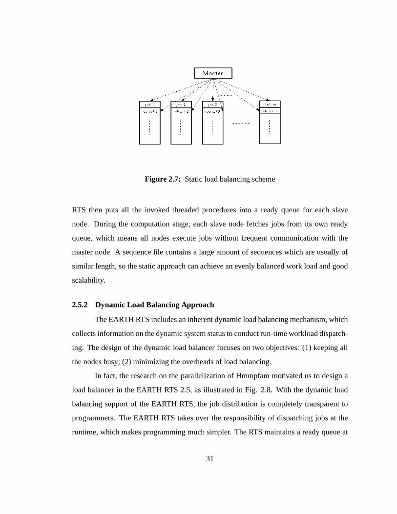
Figure 2.7: Static load balancing scheme

RTS then puts all the invoked threaded procedures into a ready queue for each slave

node. During the computation stage, each slave node fetchesjobs from its own ready

queue, which means all nodes execute jobs without frequent communication with the

master node. A sequence file contains a large amount of sequences which are usually of

similar length, so the static approach can achieve an evenlybalanced work load and good

scalability.

2.5.2 Dynamic Load Balancing Approach

The EARTH RTS includes an inherent dynamic load balancing mechanism, which

collects information on the dynamic system status to conduct run-time workload dispatch-

ing. The design of the dynamic load balancer focuses on two objectives: (1) keeping all

the nodes busy; (2) minimizing the overheads of load balancing.

In fact, the research on the parallelization of Hmmpfam motivated us to design a

load balancer in the EARTH RTS 2.5, as illustrated in Fig. 2.8. With the dynamic load

balancing support of the EARTH RTS, the job distribution is completely transparent to

programmers. The EARTH RTS takes over the responsibility ofdispatching jobs at the

runtime, which makes programming much simpler. The RTS maintains a ready queue at

31

Master

node 1 node 2

node 4 node 3

Request Job Release Job

Figure 2.8: Dynamic load balancing scheme

the master node and sends tasks to slave nodes one by one during the execution. Once

a slave node finishes a job, it requests another task from the EARTH RTS on the master

node.

The dynamic load balancing approach is more robust than the pre-determined job

assignments strategy. In the static load balancing approach, all jobs are put into the ready

queue of slave nodes during the initiation stage, and cannotbe moved away after that.

If one node has a heavier work load than others or even stops working, its jobs cannot

be reassigned to other nodes. The dynamic load balancing strategy, in contrast, is able

to avoid this situation because the EARTH RTS maintains the ready queue at the master

node. The robustness of Hmmpfam makes an important issue considering the fact that

Hmmpfam may run for quite a long time (e.g., several weeks). Also, on a supercom-

puting cluster that consists of hundreds of computing nodes, a robust approach becomes

necessary because it is not easy to guarantee that all nodes work properly without any

failure.

32

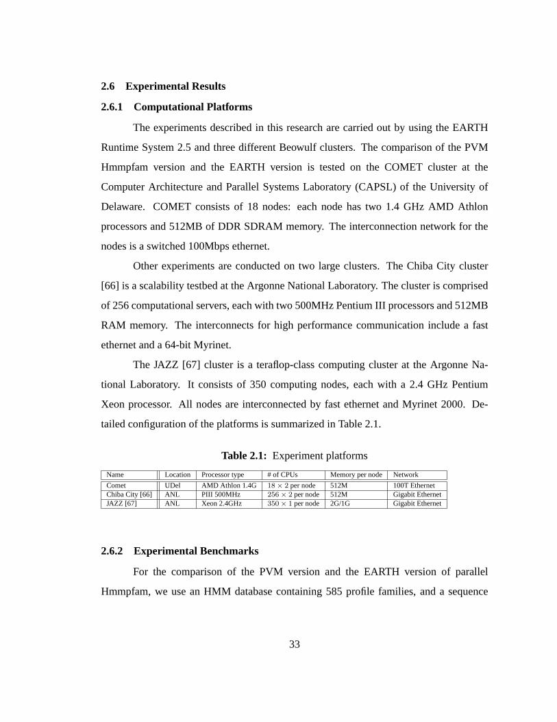
2.6 Experimental Results

2.6.1 Computational Platforms

The experiments described in this research are carried out by using the EARTH

Runtime System 2.5 and three different Beowulf clusters. The comparison of the PVM

Hmmpfam version and the EARTH version is tested on the COMET cluster at the

Computer Architecture and Parallel Systems Laboratory (CAPSL) of the University of

Delaware. COMET consists of 18 nodes: each node has two 1.4 GHzAMD Athlon

processors and 512MB of DDR SDRAM memory. The interconnection network for the

nodes is a switched 100Mbps ethernet.

Other experiments are conducted on two large clusters. The Chiba City cluster

[66] is a scalability testbed at the Argonne National Laboratory. The cluster is comprised

of 256 computational servers, each with two 500MHz Pentium III processors and 512MB

RAM memory. The interconnects for high performance communication include a fast

ethernet and a 64-bit Myrinet.

The JAZZ [67] cluster is a teraflop-class computing cluster at the Argonne Na-

tional Laboratory. It consists of 350 computing nodes, eachwith a 2.4 GHz Pentium

Xeon processor. All nodes are interconnected by fast ethernet and Myrinet 2000. De-

tailed configuration of the platforms is summarized in Table2.1.

Table 2.1: Experiment platforms

Name Location Processor type # of CPUs Memory per node Network

Comet UDel AMD Athlon 1.4G 18 × 2 per node 512M 100T EthernetChiba City [66] ANL PIII 500MHz 256 × 2 per node 512M Gigabit EthernetJAZZ [67] ANL Xeon 2.4GHz 350 × 1 per node 2G/1G Gigabit Ethernet

2.6.2 Experimental Benchmarks

For the comparison of the PVM version and the EARTH version ofparallel

Hmmpfam, we use an HMM database containing 585 profile families, and a sequence

33

file with 250 sequences. This benchmark is referred to as dataset-1 in the following

sections. Data set-1 is also used in the robustness experiment.

For testing both the static and dynamic load balancing version of EARTH Hmmp-

fam, we use an HMM database containing 50 profile families, and a sequence file con-

taining 38192 sequences. This benchmark is referred to as data set-2 in the following

sections.

2.6.3 Comparison of PVM-based and EARTH-based Implementations

The first test is conducted to compare the scalability of the PVM version and the

EARTH version on the COMET cluster using test data set-1. Fig.2.9a shows the absolute

speedup curve when both the PVM version and the EARTH versionare configured to use

only 1 CPU per node in COMET, while Fig. 2.9b shows the results for dual CPUs per

node configuration. From the figures, it is easily seen that the proposed new version has

much better scalability, especially in dual-CPU per node configuration. For example, with

16 nodes and 2 CPUs per node configuration, the absolute speedup of the PVM version is

18.50, while the speedup of our version is 30.91, which means40% reduction of execution

time. This is due to the fact that our implementation increases the computation granularity

and avoids most communication costs and internal barriers.

2.6.4 Scalability on Supercomputing Clusters

The second and third tests are conducted to show the performance of our EARTH

version Hmmpfam on large clusters, the Chiba City cluster and the JAZZ cluster, using

test data set-2. The results of both static load balancing and dynamic load balancing

schemes are shown in Fig. 2.10 to Fig. 2.11, where Fig. 2.10a and Fig. 2.10b show the

results for static load balancing on 1 CPU per node and 2 CPUs pernode configuration,

and Fig. 2.11a and Fig. 2.11b are the results for dynamic loadbalancing. The two

methods do not have much difference in the absolute speedup.This is due to the fact

that subtasks are relatively similar in size, which means static load balancing can also

34

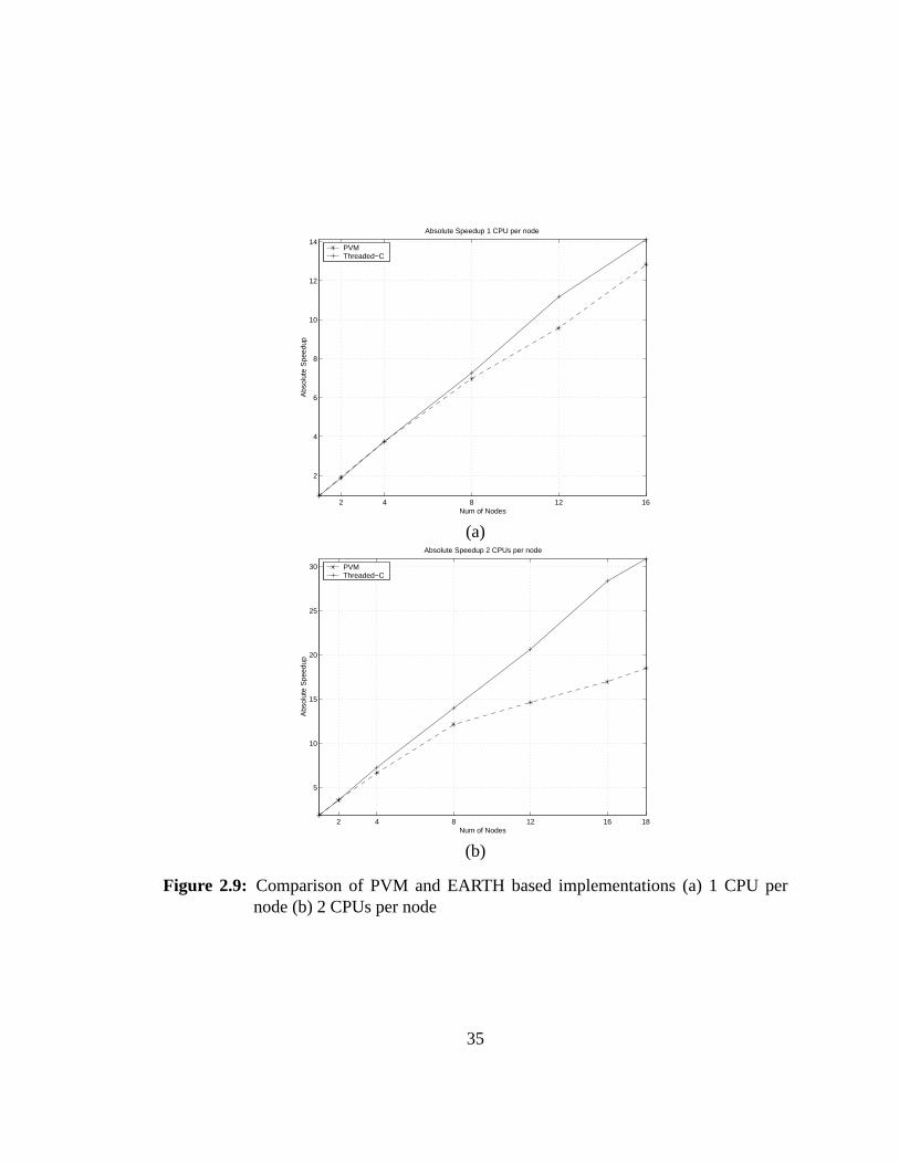
2 4 8 12 16

2

4

6

8

10

12

14

Num of Nodes

Abs

olut

e S

peed

up

Absolute Speedup 1 CPU per node

PVMThreaded−C

(a)

2 4 8 12 16 18

5

10

15

20

25

30

Num of Nodes

Abs

olut

e S

peed

up

Absolute Speedup 2 CPUs per node

PVMThreaded−C

(b)

Figure 2.9: Comparison of PVM and EARTH based implementations (a) 1 CPU pernode (b) 2 CPUs per node

35

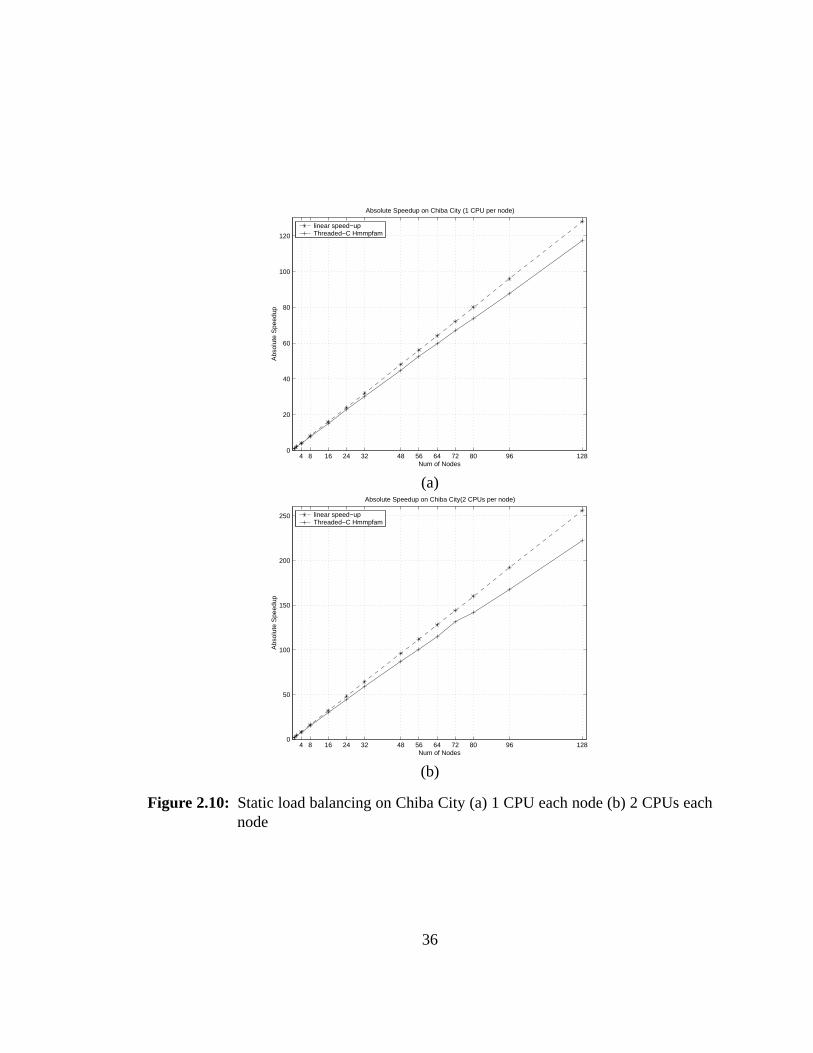
4 8 16 24 32 48 56 64 72 80 96 1280

20

40

60

80

100

120

Absolute Speedup on Chiba City (1 CPU per node)

Num of Nodes

Abs

olut

e S

peed

up

linear speed−upThreaded−C Hmmpfam

(a)

4 8 16 24 32 48 56 64 72 80 96 1280

50

100

150

200

250

Absolute Speedup on Chiba City(2 CPUs per node)

Num of Nodes

Abs

olut

e S

peed

up

linear speed−upThreaded−C Hmmpfam

(b)

Figure 2.10: Static load balancing on Chiba City (a) 1 CPU each node (b) 2 CPUs eachnode

36

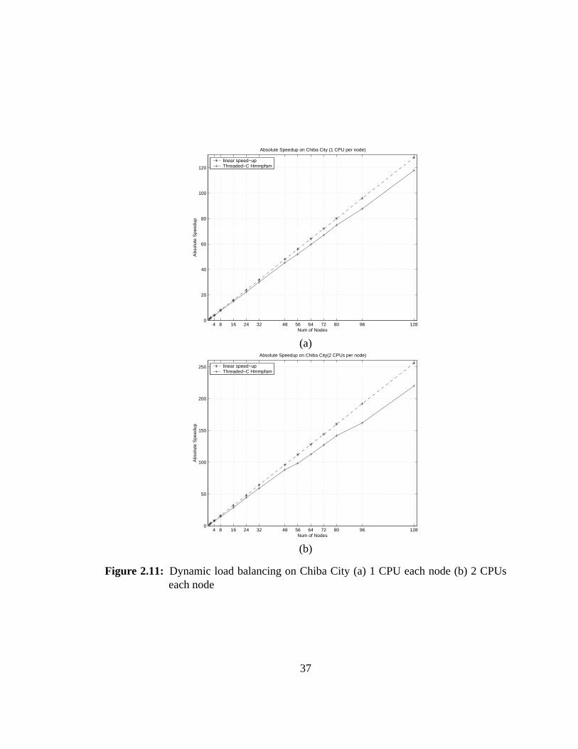
4 8 16 24 32 48 56 64 72 80 96 1280

20

40

60

80

100

120

Absolute Speedup on Chiba City (1 CPU per node)

Num of Nodes

Abs

olut

e S

peed

up

linear speed−upThreaded−C Hmmpfam

(a)

4 8 16 24 32 48 56 64 72 80 96 1280

50

100

150

200

250

Absolute Speedup on Chiba City(2 CPUs per node)

Num of Nodes

Abs

olut

e S

peed

up

linear speed−upThreaded−C Hmmpfam

(b)

Figure 2.11: Dynamic load balancing on Chiba City (a) 1 CPU each node (b) 2 CPUseach node

37

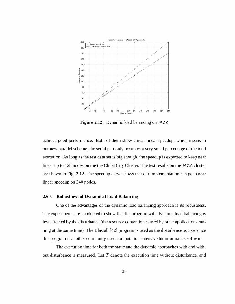
16 32 56 80 96 128 144 160 180 200 220 240

20

40

60

80

100

120

140

160

180

200

220

240

Num of Nodes

Abs

olut

e S

peed

up

Absolute Speedup on JAZZ(1 CPU per node)

linear speed−upThreaded−C Hmmpfam

Figure 2.12: Dynamic load balancing on JAZZ

achieve good performance. Both of them show a near linear speedup, which means in

our new parallel scheme, the serial part only occupies a verysmall percentage of the total

execution. As long as the test data set is big enough, the speedup is expected to keep near

linear up to 128 nodes on the the Chiba City Cluster. The test results on the JAZZ cluster

are shown in Fig. 2.12. The speedup curve shows that our implementation can get a near

linear speedup on 240 nodes.

2.6.5 Robustness of Dynamical Load Balancing

One of the advantages of the dynamic load balancing approachis its robustness.

The experiments are conducted to show that the program with dynamic load balancing is

less affected by the disturbance (the resource contention caused by other applications run-

ning at the same time). The Blastall [42] program is used as thedisturbance source since

this program is another commonly used computation-intensive bioinformatics software.

The execution time for both the static and the dynamic approaches with and with-

out disturbance is measured. LetT denote the execution time without disturbance, and

38

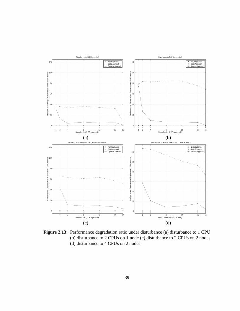
1 2 4 8 12 16 18

0

20

40

60

80

100

120

Disturbance to 1 CPU on node 1

Num of nodes (2 CPUs per node)

Pe

rfo

rma

nce

De

gra

da

tio

n R

atio

un

de

r D

istu

rba

nce

No DisturbanceStatic ApproachDynamic Approach

1 2 4 8 12 16 18

0

20

40

60

80

100

120

Disturbance to 2 CPUs on node 1

Num of nodes (2 CPUs per node)P

erf

orm

an

ce

De

gra

da

tio

n R

atio

n u

nd

er

Dis

turb

an

ce

No DisturbanceStatic ApproachDynamic Approach

(a) (b)

2 4 8 12 16 18

0

20

40

60

80

100

120

Disturbance to 1 CPU on node 1, and 1 CPU on node 2

Num of nodes (2 CPUs per node)

Pe

rfo

rma

nce

De

gra

da

tio

n R

atio

un

de

r D

istu

rba

nce

No DisturbanceStatic ApproachDynamic Approach

2 4 8 12 16 18

0

20

40

60

80

100

120

Disturbance to 2 CPUs on node 1 and 2 CPUs on node 2

Num of nodes (2 CPUs per node)

Pe

rfo

rma

nce

De

gra

da

tio

n R

atio

un

de

r D

istu

rba

nce

No DisturbanceStatic ApproachDynamic Approach

(c) (d)

Figure 2.13: Performance degradation ratio under disturbance (a) disturbance to 1 CPU(b) disturbance to 2 CPUs on 1 node (c) disturbance to 2 CPUs on 2 nodes(d) disturbance to 4 CPUs on 2 nodes

39

T ′ denote the execution time with disturbance. Define theperformance degradation ratio

under disturbance(PDRD) as:

PDRD = (T ′ − T

T) × 100% (2.5)

The PDRD is computed and plotted for both the static and the dynamic approaches. A

smaller PDRD indicates that the performance is less influenced by the introduction of

disturbance, thus implying the higher implementation robustness.

For the robustness experiment, the data set-1 is used on the COMET cluster. Fig.

2.13a shows the result when only one Blastall program is running on 1 CPU to disturb

the execution of Hmmpfam, and Fig. 2.13b shows the result when two CPUs of one node

are both disturbed. Fig. 2.13c and Fig. 2.13d show the resultwhen 2 computing nodes

are disturbed. From the figures, it is apparent that the dynamic load balancing program is

less affected by the disturbance and thus has higher robustness.

2.7 Summary

We implemented a new cluster-based solution of the HMM database searching

tool on the EARTH model and demonstrated significant performance improvement over

the original parallel version based on PVM. Our solution provides near linear scalability

on supercomputing clusters. Comparison between the static and dynamic load balancing

approaches shows that the latter is a more robust and practical solution for large-scale

time-consuming applications running on clusters.

This new implementation allows researchers to analyze biological sequences at a

much higher speed and also makes it possible for scientists to analyze problems that were

previously considered too large and too time consuming. Theparallelization implemen-

tation in this work motivated the addition of a robust dynamic load balancing support into

the EARTH model, which proves that applications could be thedriving force for design

of architecture and programming models.

40

Chapter 3

SPACE RIP TARGETED TO CELLULAR COMPUTER

ARCHITECTURE CYCLOPS-64

3.1 Introduction

This chapter presents the parallelization and performanceoptimization of another

biomedical application–SPACE RIP, a parallel imaging technique on the Cyclops-64

multiprocessor-on-a-chip computer architecture. Cyclops-64 [10–12, 34, 35] is a new ar-

chitecture being developed at the IBM T. J. Watson Research Center and the University

of Delaware. SPACE RIP (Sensitivity Profiles From an Array of Coils for Encoding and

Reconstruction in Parallel) is one of the parallel imaging techniques which use spatial

information contained in the component coils of an array to partially replace spatial en-

coding which would normally be performed using gradients inorder to reduce imaging

acquisition time. We present the parallelization and optimization of SPACE RIP at three

levels. The top level is the loop level parallelization. Theloop level parallelization decom-

poses SPACE RIP into many SVD problems. This is possible because the reconstructions

of each column in an image are independent of each other. The reconstruction of each

column is a pseudoinverse of a matrix, which is solved by the singular value decompo-

sition (SVD). The middle level is the parallelization of a SVD problem using one-sided

Jacobi algorithm and is implemented on Cyclops-64. At this level, an SVD problem is

decomposed into many tasks, each one of them is a matrix column rotation routine. The

bottom level further optimizes the matrix column rotation routine by using several mem-

ory preloading or loop unrolling approaches.

41

1. We implemented the parallelization and optimization of SPACE RIP at three lev-

els. The top level is the loop level parallelization, which decomposes SPACE RIP

into many tasks of a singular value decomposition (SVD) problem. The middle

level parallelizes the SVD problem using the one-sided Jacobi algorithm and is

implemented on Cyclops-64. At this level, an SVD problem is decomposed into

many matrix column rotation routines. The bottom level further optimizes the ma-

trix column rotation routine using several memory preloading or loop unrolling

approaches.

2. We developed a model and trace analyzer to decompose the total execution cycles

into four parts: total instruction counts, “DLL”, “DLF” and“DLI”, where “DLL”

represents the cycles spent on memory access, “DLF” represents the latency cy-

cles related to floating point operations, and “DLI” represents the latency cycles

related to integer operations. This simple model allows us to study the application

performance tradeoff for different algorithms.

3. Using a few application parameters such as matrix size, group size, and architec-

tural parameters such as onchip and offchip latency, we developed analytical equa-

tions for comparing different memory access approaches such as preloading and

loop unrolling. We used a cycle accurate simulator to validate the analysis and

compare the effect of different approaches on the “DLL” partand the total execu-

tion cycles.

The remainder of this chapter is organized as follows. The target platform

Cyclops-64 is introduced in Section 3.2. The background of MRIimaging is presented

in Section.3.3. The SPACE RIP technique is briefly reviewed in section 3.4 to expose the

parallelism inherent in the problem. The coarse grain loop level parallelization is pre-

sented in Section 3.5, and the fine grain parallelization of the SVD algorithm is presented

in Section 3.6. Different memory access approaches are introduced in Section 3.7 in order

42

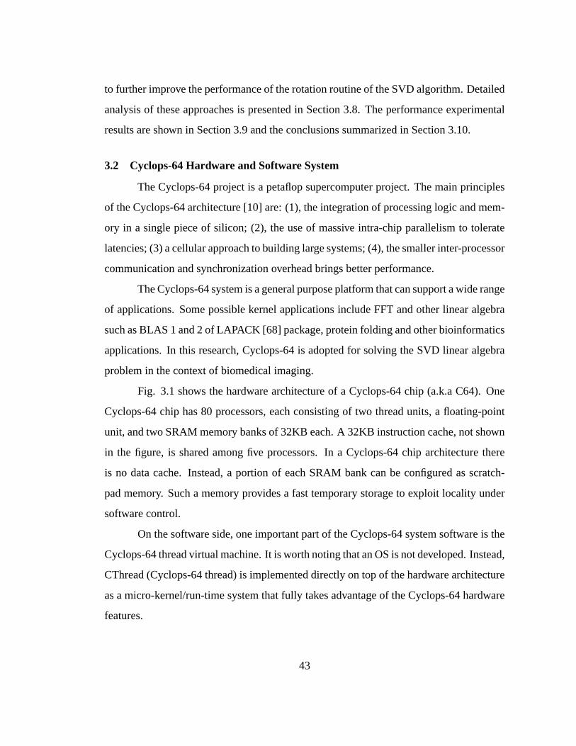
to further improve the performance of the rotation routine of the SVD algorithm. Detailed

analysis of these approaches is presented in Section 3.8. The performance experimental

results are shown in Section 3.9 and the conclusions summarized in Section 3.10.

3.2 Cyclops-64 Hardware and Software System

The Cyclops-64 project is a petaflop supercomputer project. The main principles

of the Cyclops-64 architecture [10] are: (1), the integration of processing logic and mem-

ory in a single piece of silicon; (2), the use of massive intra-chip parallelism to tolerate

latencies; (3) a cellular approach to building large systems; (4), the smaller inter-processor

communication and synchronization overhead brings betterperformance.

The Cyclops-64 system is a general purpose platform that can support a wide range

of applications. Some possible kernel applications include FFT and other linear algebra

such as BLAS 1 and 2 of LAPACK [68] package, protein folding and other bioinformatics

applications. In this research, Cyclops-64 is adopted for solving the SVD linear algebra

problem in the context of biomedical imaging.

Fig. 3.1 shows the hardware architecture of a Cyclops-64 chip(a.k.a C64). One

Cyclops-64 chip has 80 processors, each consisting of two thread units, a floating-point

unit, and two SRAM memory banks of 32KB each. A 32KB instruction cache, not shown

in the figure, is shared among five processors. In a Cyclops-64 chip architecture there

is no data cache. Instead, a portion of each SRAM bank can be configured as scratch-

pad memory. Such a memory provides a fast temporary storage to exploit locality under

software control.

On the software side, one important part of the Cyclops-64 system software is the

Cyclops-64 thread virtual machine. It is worth noting that anOS is not developed. Instead,

CThread (Cyclops-64 thread) is implemented directly on top ofthe hardware architecture

as a micro-kernel/run-time system that fully takes advantage of the Cyclops-64 hardware

features.

43

Mem

ory

Off−

chip

Mem

ory

Off−

chip

Mem

ory

Off−

chip

Mem

ory

Off−

chip

TU

FP

SP SP

TU TU

FP

SP SP

TU TU

FP

SP SP

TU TU

FP

SP SP

TU

GM GM GM GM GM GM GM GM

Chip

A−

switc

h

Processor

Board

ethe

rnet

Gig

abit

HD

3D−

mes

h

ATA

Crossbar Network

Figure 3.1: Cyclops-64 chip

The Cyclops-64 thread virtual machine includes a thread model, a memory model

and a synchronization model. The Cyclops-64 chip hardware supports a shared address

space model: all onchip SRAM and offchip DRAM banks are addressable from all thread

units/processors on the same chip, which means that all the threads can see a single shared

address space. More details are explained in [34, 35, 69].

In the thread synchronization model, the CThread mutex lock and unlock opera-

tions are directly implemented using Cyclops-64 hardware atomic test-and-set operations

and are thus very efficient. Furthermore, a very efficient barrier synchronization primitive

is provided. Barriers are implemented using the “Signal Bus” special purpose register.

The barrier function can be invoked by a group of threads. Threads will block until all the

threads participating in the operation have reached this routine.

The memory organization is summarized in Table 3.1. The default offchip latency

is 36 cycles. It can become larger when there is a heavy load ofmemory accesses from

many thread units. This parameter can be preset in the Cyclops-64 simulator. In this

experiment, the offchip latency is set to be 36 or 80.

Another set of parameters in the Cyclops-64 simulator is the delay of instructions.

The delay for an instruction is decomposed in two parts, execution cycles and latency

cycles. The execution unit is kept busy for the number of execution cycles and another

instruction cannot be issued during the execution cycles. The result is available after the

number of execution+latency cycles. The resources can, however, be utilized by other

44

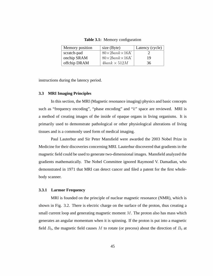
Table 3.1: Memory configuration

Memory position size (Byte) Latency (cycle)scratch-pad 80×2bank×16K 2onchip SRAM 80×2bank×16K 19offchip DRAM 4bank × 512M 36

instructions during the latency period.

3.3 MRI Imaging Principles

In this section, the MRI (Magnetic resonance imaging) physics and basic concepts

such as “frequency encoding”, “phase encoding” and “k” space are reviewed. MRI is

a method of creating images of the inside of opaque organs in living organisms. It is

primarily used to demonstrate pathological or other physiological alterations of living

tissues and is a commonly used form of medical imaging.

Paul Lauterbur and Sir Peter Mansfield were awarded the 2003 Nobel Prize in

Medicine for their discoveries concerning MRI. Lauterbur discovered that gradients in the

magnetic field could be used to generate two-dimensional images. Mansfield analyzed the

gradients mathematically. The Nobel Committee ignored Raymond V. Damadian, who

demonstrated in 1971 that MRI can detect cancer and filed a patent for the first whole-

body scanner.

3.3.1 Larmor Frequency

MRI is founded on the principle of nuclear magnetic resonance(NMR), which is

shown in Fig. 3.2. There is electric charge on the surface of the proton, thus creating a

small current loop and generating magnetic momentM . The proton also has mass which

generates an angular momentum when it is spinning. If the proton is put into a magnetic

field B0, the magnetic field causesM to rotate (or precess) about the direction ofB0 at

45

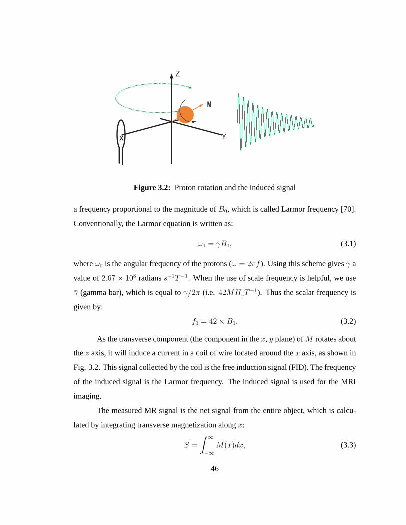
x Y

Z

Figure 3.2: Proton rotation and the induced signal

a frequency proportional to the magnitude ofB0, which is called Larmor frequency [70].

Conventionally, the Larmor equation is written as:

ω0 = γB0, (3.1)

whereω0 is the angular frequency of the protons (ω = 2πf ). Using this scheme givesγ a

value of2.67 × 108 radianss−1T−1. When the use of scale frequency is helpful, we use

γ (gamma bar), which is equal toγ/2π (i.e. 42MHzT−1). Thus the scalar frequency is

given by:

f0 = 42 × B0. (3.2)

As the transverse component (the component in thex, y plane) ofM rotates about

thez axis, it will induce a current in a coil of wire located aroundthex axis, as shown in

Fig. 3.2. This signal collected by the coil is the free induction signal (FID). The frequency

of the induced signal is the Larmor frequency. The induced signal is used for the MRI

imaging.

The measured MR signal is the net signal from the entire object, which is calcu-

lated by integrating transverse magnetization alongx:

S =

∫ ∞

−∞M(x)dx, (3.3)

46

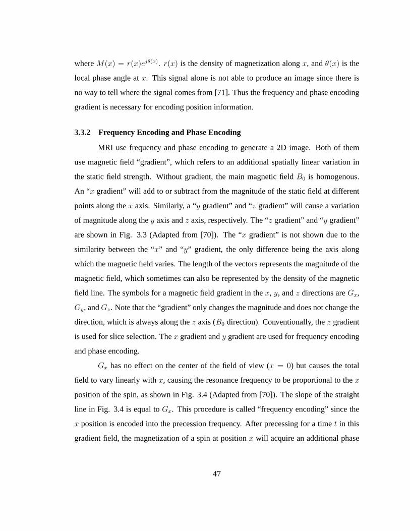
whereM(x) = r(x)ejθ(x). r(x) is the density of magnetization alongx, andθ(x) is the

local phase angle atx. This signal alone is not able to produce an image since thereis

no way to tell where the signal comes from [71]. Thus the frequency and phase encoding

gradient is necessary for encoding position information.

3.3.2 Frequency Encoding and Phase Encoding

MRI use frequency and phase encoding to generate a 2D image. Both of them

use magnetic field “gradient”, which refers to an additionalspatially linear variation in

the static field strength. Without gradient, the main magnetic field B0 is homogenous.

An “x gradient” will add to or subtract from the magnitude of the static field at different

points along thex axis. Similarly, a “y gradient” and “z gradient” will cause a variation

of magnitude along they axis andz axis, respectively. The “z gradient” and “y gradient”

are shown in Fig. 3.3 (Adapted from [70]). The “x gradient” is not shown due to the

similarity between the “x” and “y” gradient, the only difference being the axis along

which the magnetic field varies. The length of the vectors represents the magnitude of the

magnetic field, which sometimes can also be represented by the density of the magnetic

field line. The symbols for a magnetic field gradient in thex, y, andz directions areGx,

Gy, andGz. Note that the “gradient” only changes the magnitude and does not change the

direction, which is always along thez axis (B0 direction). Conventionally, thez gradient

is used for slice selection. Thex gradient andy gradient are used for frequency encoding

and phase encoding.

Gx has no effect on the center of the field of view (x = 0) but causes the total

field to vary linearly withx, causing the resonance frequency to be proportional to thex

position of the spin, as shown in Fig. 3.4 (Adapted from [70]). The slope of the straight

line in Fig. 3.4 is equal toGx. This procedure is called “frequency encoding” since the

x position is encoded into the precession frequency. After precessing for a timet in this

gradient field, the magnetization of a spin at positionx will acquire an additional phase

47

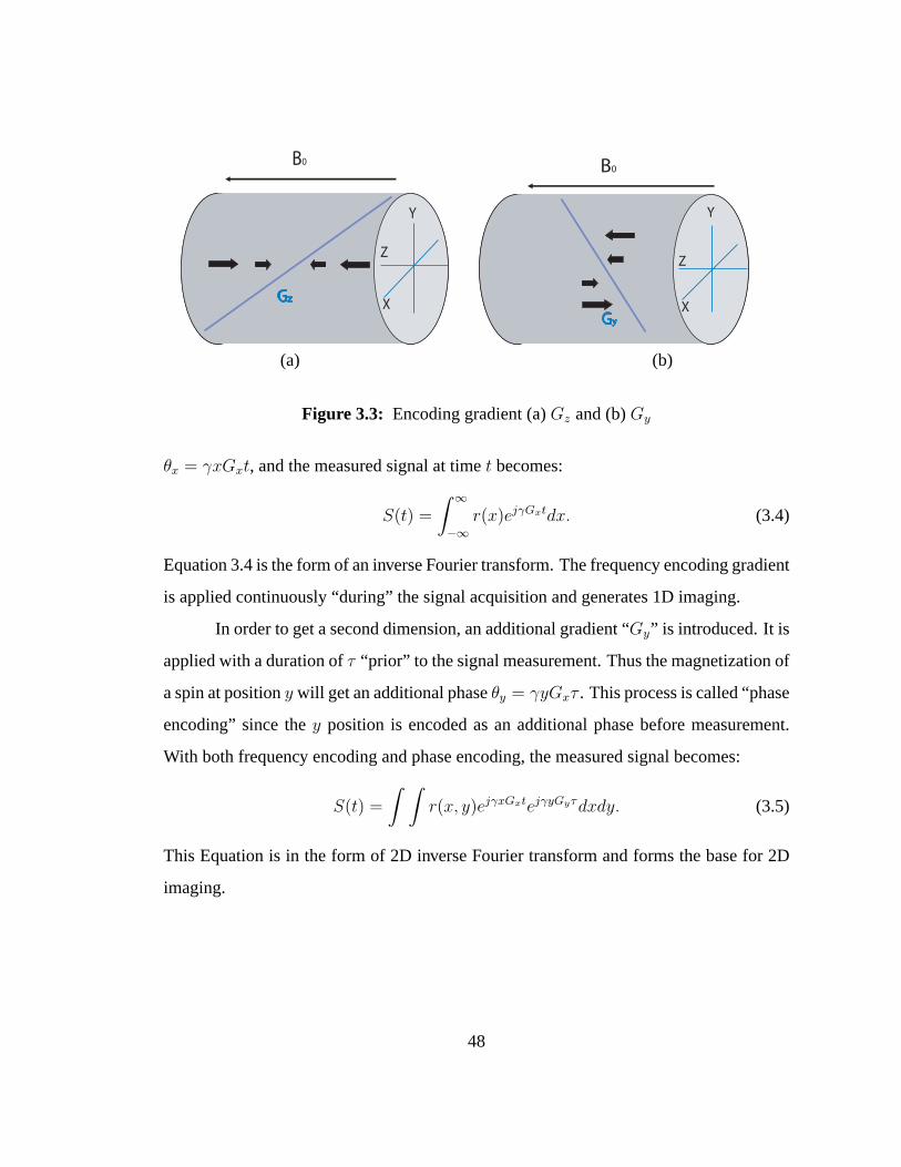
B0

GzX

Y

Z

B0

Gy

X

Y

Z

(a) (b)

Figure 3.3: Encoding gradient (a)Gz and (b)Gy

θx = γxGxt, and the measured signal at timet becomes:

S(t) =

∫ ∞

−∞r(x)ejγGxtdx. (3.4)

Equation 3.4 is the form of an inverse Fourier transform. Thefrequency encoding gradient

is applied continuously “during” the signal acquisition and generates 1D imaging.

In order to get a second dimension, an additional gradient “Gy” is introduced. It is

applied with a duration ofτ “prior” to the signal measurement. Thus the magnetization of

a spin at positiony will get an additional phaseθy = γyGxτ . This process is called “phase

encoding” since they position is encoded as an additional phase before measurement.

With both frequency encoding and phase encoding, the measured signal becomes:

S(t) =

∫ ∫

r(x, y)ejγxGxtejγyGyτdxdy. (3.5)

This Equation is in the form of 2D inverse Fourier transform and forms the base for 2D

imaging.

48

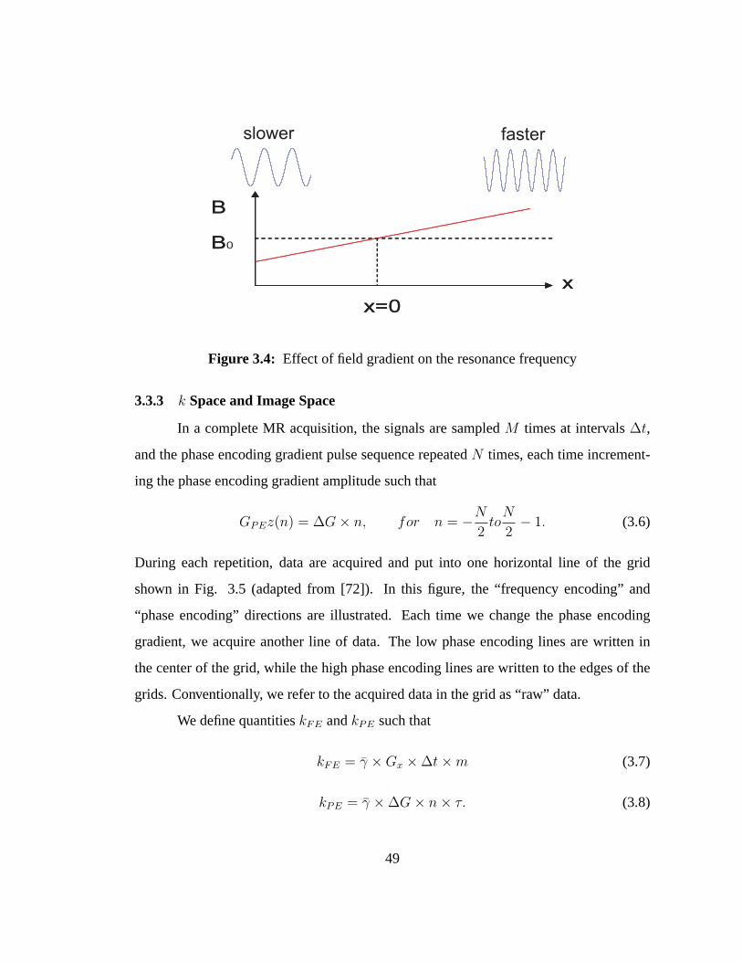
B

B

x=0

x

B

B0

x=0

x

slower faster

Figure 3.4: Effect of field gradient on the resonance frequency

3.3.3 k Space and Image Space

In a complete MR acquisition, the signals are sampledM times at intervals∆t,

and the phase encoding gradient pulse sequence repeatedN times, each time increment-

ing the phase encoding gradient amplitude such that

GPEz(n) = ∆G × n, for n = −N

2to

N

2− 1. (3.6)

During each repetition, data are acquired and put into one horizontal line of the grid

shown in Fig. 3.5 (adapted from [72]). In this figure, the “frequency encoding” and

“phase encoding” directions are illustrated. Each time we change the phase encoding

gradient, we acquire another line of data. The low phase encoding lines are written in

the center of the grid, while the high phase encoding lines are written to the edges of the

grids. Conventionally, we refer to the acquired data in the grid as “raw” data.

We define quantitieskFE andkPE such that

kFE = γ × Gx × ∆t × m (3.7)

kPE = γ × ∆G × n × τ. (3.8)

49

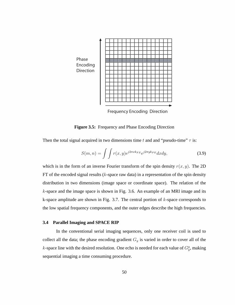
Frequency Encoding Direction

Phase

Encoding

Direction

Figure 3.5: Frequency and Phase Encoding Direction

Then the total signal acquired in two dimensions timet and and “pseudo-time”τ is:

S(m,n) =

∫ ∫

r(x, y)ej2πxkFEej2πykPEdxdy, (3.9)

which is in the form of an inverse Fourier transform of the spin densityr(x, y). The 2D

FT of the encoded signal results (k-space raw data) in a representation of the spin density

distribution in two dimensions (image space or coordinate space). The relation of the

k-space and the image space is shown in Fig. 3.6. An example of an MRI image and its

k-space amplitude are shown in Fig. 3.7. The central portionof k-space corresponds to

the low spatial frequency components, and the outer edges describe the high frequencies.

3.4 Parallel Imaging and SPACE RIP

In the conventional serial imaging sequences, only one receiver coil is used to

collect all the data; the phase encoding gradientGy is varied in order to cover all of the

k-space line with the desired resolution. One echo is needed for each value ofGgy, making

sequential imaging a time consuming procedure.

50

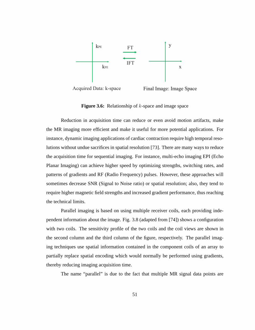
FT

IFTkkFEFE

kkPEPE

Acquired Data: k-space

xx

yy

Final Image: Image SpaceFinal Image: Image Space

Figure 3.6: Relationship ofk-space and image space

Reduction in acquisition time can reduce or even avoid motionartifacts, make

the MR imaging more efficient and make it useful for more potential applications. For

instance, dynamic imaging applications of cardiac contraction require high temporal reso-

lutions without undue sacrifices in spatial resolution [73]. There are many ways to reduce

the acquisition time for sequential imaging. For instance,multi-echo imaging EPI (Echo

Planar Imaging) can achieve higher speed by optimizing strengths, switching rates, and

patterns of gradients and RF (Radio Frequency) pulses. However, these approaches will

sometimes decrease SNR (Signal to Noise ratio) or spatial resolution; also, they tend to

require higher magnetic field strengths and increased gradient performance, thus reaching

the technical limits.

Parallel imaging is based on using multiple receiver coils,each providing inde-

pendent information about the image. Fig. 3.8 (adapted from[74]) shows a configuration

with two coils. The sensitivity profile of the two coils and the coil views are shown in

the second column and the third column of the figure, respectively. The parallel imag-

ing techniques use spatial information contained in the component coils of an array to

partially replace spatial encoding which would normally beperformed using gradients,

thereby reducing imaging acquisition time.

The name “parallel” is due to the fact that multiple MR signaldata points are

51

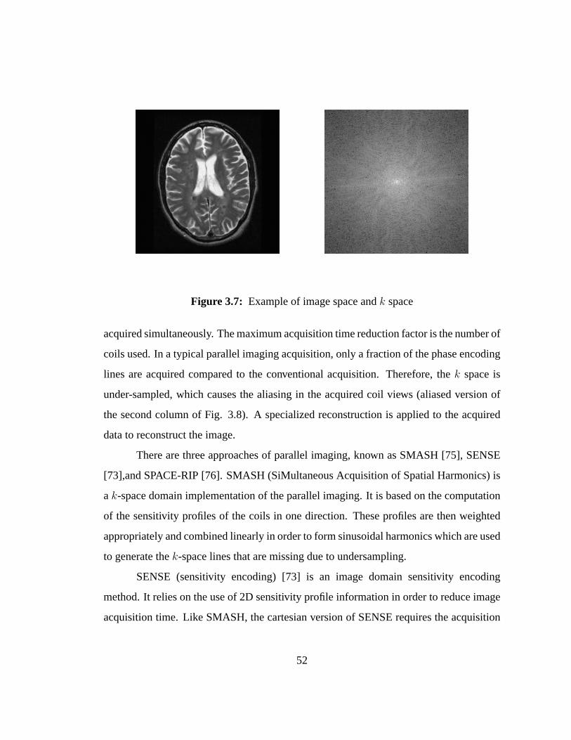
Figure 3.7: Example of image space andk space

acquired simultaneously. The maximum acquisition time reduction factor is the number of

coils used. In a typical parallel imaging acquisition, onlya fraction of the phase encoding

lines are acquired compared to the conventional acquisition. Therefore, thek space is

under-sampled, which causes the aliasing in the acquired coil views (aliased version of

the second column of Fig. 3.8). A specialized reconstruction is applied to the acquired

data to reconstruct the image.

There are three approaches of parallel imaging, known as SMASH [75], SENSE

[73],and SPACE-RIP [76]. SMASH (SiMultaneous Acquisition ofSpatial Harmonics) is

ak-space domain implementation of the parallel imaging. It isbased on the computation

of the sensitivity profiles of the coils in one direction. These profiles are then weighted

appropriately and combined linearly in order to form sinusoidal harmonics which are used

to generate thek-space lines that are missing due to undersampling.

SENSE (sensitivity encoding) [73] is an image domain sensitivity encoding

method. It relies on the use of 2D sensitivity profile information in order to reduce image

acquisition time. Like SMASH, the cartesian version of SENSE requires the acquisition

52

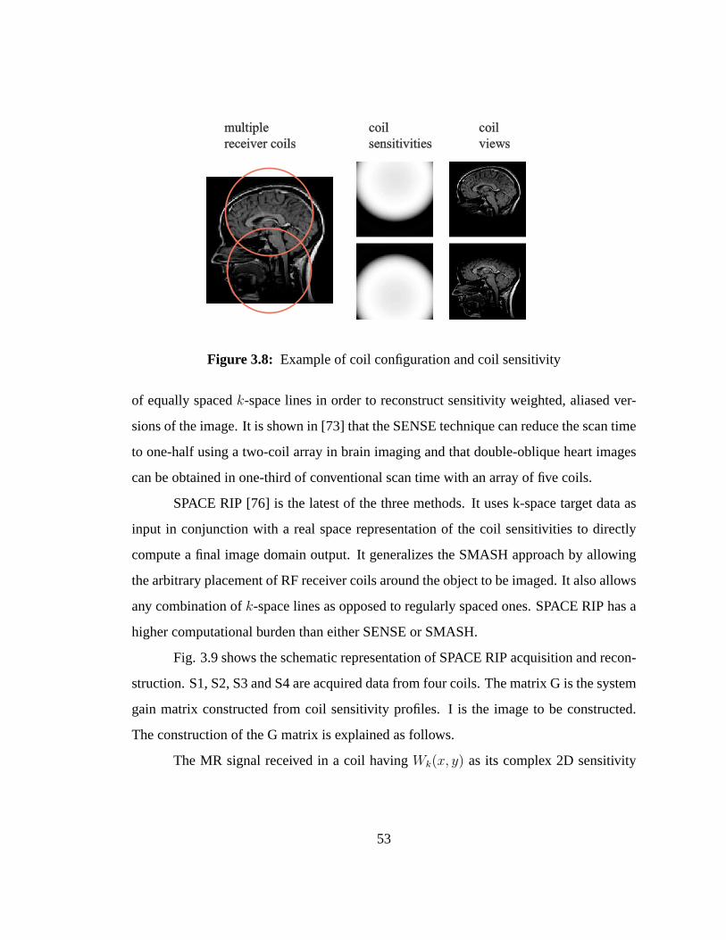
coil

views

coil

sensitivities

multiple

receiver coils

Figure 3.8: Example of coil configuration and coil sensitivity

of equally spacedk-space lines in order to reconstruct sensitivity weighted,aliased ver-

sions of the image. It is shown in [73] that the SENSE technique can reduce the scan time

to one-half using a two-coil array in brain imaging and that double-oblique heart images

can be obtained in one-third of conventional scan time with an array of five coils.

SPACE RIP [76] is the latest of the three methods. It uses k-space target data as

input in conjunction with a real space representation of thecoil sensitivities to directly

compute a final image domain output. It generalizes the SMASHapproach by allowing

the arbitrary placement of RF receiver coils around the object to be imaged. It also allows

any combination ofk-space lines as opposed to regularly spaced ones. SPACE RIP hasa

higher computational burden than either SENSE or SMASH.

Fig. 3.9 shows the schematic representation of SPACE RIP acquisition and recon-

struction. S1, S2, S3 and S4 are acquired data from four coils. The matrix G is the system

gain matrix constructed from coil sensitivity profiles. I isthe image to be constructed.

The construction of the G matrix is explained as follows.

The MR signal received in a coil havingWk(x, y) as its complex 2D sensitivity

53

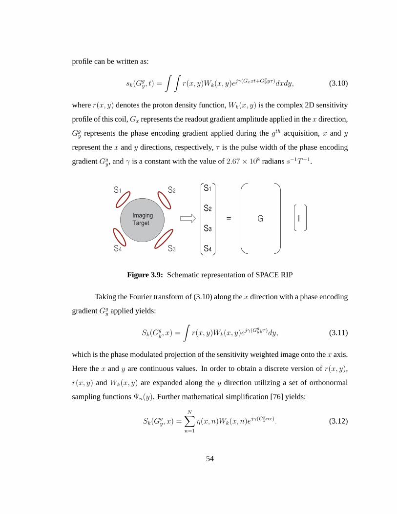
profile can be written as:

sk(Ggy, t) =

∫ ∫

r(x, y)Wk(x, y)ejγ(Gxxt+Ggyyτ)dxdy, (3.10)

wherer(x, y) denotes the proton density function,Wk(x, y) is the complex 2D sensitivity

profile of this coil,Gx represents the readout gradient amplitude applied in thex direction,

Ggy represents the phase encoding gradient applied during thegth acquisition,x andy

represent thex andy directions, respectively,τ is the pulse width of the phase encoding

gradientGgy, andγ is a constant with the value of2.67 × 108 radianss−1T−1.

Imaging

Target

Figure 3.9: Schematic representation of SPACE RIP

Taking the Fourier transform of (3.10) along thex direction with a phase encoding

gradientGgy applied yields:

Sk(Ggy, x) =

∫

r(x, y)Wk(x, y)ejγ(Ggyyτ)dy, (3.11)

which is the phase modulated projection of the sensitivity weighted image onto thex axis.

Here thex andy are continuous values. In order to obtain a discrete versionof r(x, y),

r(x, y) andWk(x, y) are expanded along they direction utilizing a set of orthonormal

sampling functionsΨn(y). Further mathematical simplification [76] yields:

Sk(Ggy, x) =

N∑

n=1

η(x, n)Wk(x, n)ejγ(Ggynτ). (3.12)

54

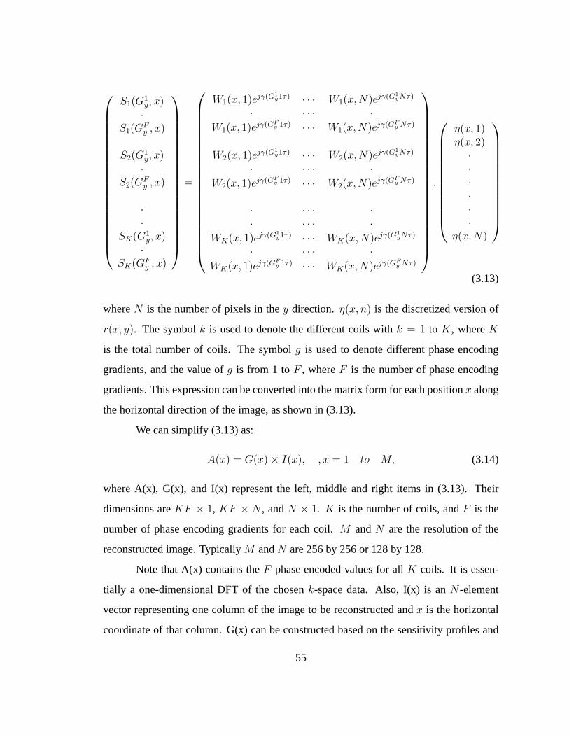
S1(G1y, x)·

S1(GFy , x)

S2(G1y, x)·

S2(GFy , x)

··

SK(G1y, x)·

SK(GFy , x)

=

W1(x, 1)ejγ(G1y1τ) · · · W1(x,N)ejγ(G1

yNτ)

· · · · ·

W1(x, 1)ejγ(GFy 1τ) · · · W1(x,N)ejγ(GF

y Nτ)

W2(x, 1)ejγ(G1y1τ) · · · W2(x,N)ejγ(G1

yNτ)

· · · · ·

W2(x, 1)ejγ(GFy 1τ) · · · W2(x,N)ejγ(GF

y Nτ)

· · · · ·· · · · ·

WK(x, 1)ejγ(G1y1τ) · · · WK(x,N)ejγ(G1

yNτ)

· · · · ·

WK(x, 1)ejγ(GFy 1τ) · · · WK(x,N)ejγ(GF

y Nτ)

.

η(x, 1)η(x, 2)

······

η(x,N)

(3.13)

whereN is the number of pixels in they direction. η(x, n) is the discretized version of

r(x, y). The symbolk is used to denote the different coils withk = 1 to K, whereK

is the total number of coils. The symbolg is used to denote different phase encoding

gradients, and the value ofg is from 1 toF , whereF is the number of phase encoding

gradients. This expression can be converted into the matrixform for each positionx along

the horizontal direction of the image, as shown in (3.13).

We can simplify (3.13) as:

A(x) = G(x) × I(x), , x = 1 to M, (3.14)

where A(x), G(x), and I(x) represent the left, middle and right items in (3.13). Their

dimensions areKF × 1, KF × N , andN × 1. K is the number of coils, andF is the

number of phase encoding gradients for each coil.M andN are the resolution of the

reconstructed image. TypicallyM andN are 256 by 256 or 128 by 128.

Note that A(x) contains theF phase encoded values for allK coils. It is essen-

tially a one-dimensional DFT of the chosenk-space data. Also, I(x) is anN -element

vector representing one column of the image to be reconstructed andx is the horizontal

coordinate of that column. G(x) can be constructed based on the sensitivity profiles and

55

phase encodes used. If an image hasM columns, thenx ranges from 1 toM . For each

particularx, we have an equation such as (3.14). TheseM equations can be constructed

and solved independently of each other, which means each column of the image can be

reconstructed independent of each other. IncreasingM andN increases the computa-

tion load. It can also be seen that the Gain matrix G(x) becomes larger whenK andF

increase, thus increasing the computation load.

3.5 Loop Level Parallelization

In this section, the coarse grain parallelization of the image reconstruction is pre-

sented. As shown in the previous section, the SPACE RIP reconstruction algorithm is

computed column by column. The algorithm begins by reading k-space data from the

data file, then a 1D DFT is computed along thex direction, followed by a major loop

reconstructing the columns one by one. This loop hasM iterations, whereM is thex

dimension of the reconstructed image. Inside each iteration, a matrixG(x), as in (3.13)

is constructed. The pseudoinverse of this matrix is then computed, and one column of

the image is finally reconstructed by multiplying the inverse matrix with the vectorA(X)

as in (3.13). Timing profiling of the program for a typical data set shows that the major

loop occupies about 98.79 % of the total execution time. Accordingly, this loop is the

bottleneck to be parallelized.

Both Pthread and OpenMP versions at the loop level are implemented. The

speedup result on a 12 CPUs Sunfire workstation are shown in section 3.9. On a shared-

memory multiprocessor computer, all CPUs share the same mainmemory and can work

on the same data concurrently. The major advantage of the shared-memory machine is

that no explicit message-passing is needed, thus making it easier for programmers to par-

allelize the sequential code of an application compared to message-passing-based parallel

languages, such as PVM or MPI.

Multithreaded programming is a programming paradigm tailored to shared-

memory multiprocessor systems. Multithreaded programming offers an alternative to

56

multi-process programming that is typically less demanding of system resources – here

the collection of interacting tasks are implemented as multiple threads within a single

process. The programmer can regard the individual threads as running concurrently and

need not implement task switching explicitly, which is instead handled by the operating

system or thread library in a manner similar to that for task switching between processes.

Libraries and operating system support for multithreaded programming are available to-

day on most platforms, including almost all available Unix variants. However, it is worth

noting that there is a certain amount of overhead for handling multiple threads, so the

performance gain archived by parallelization must outweigh this overhead. In our ap-

plication, the loop level parallelizations are at the coarse grain level, thus justifying the

overhead.

Pthread [31] is a standardized model for dividing a program into subtasks whose

executions can be interleaved or run in parallel. The OpenMPApplication Program Inter-

face (API) [77] supports multi-platform shared-memory parallel programming in C/C++

and Fortran on almost all architectures. Additionally, it is a portable, scalable model that

gives shared-memory parallel programmers a simple and flexible interface for developing

parallel applications.

It is worth noting that static variables are shared across all threads for both Pthread

and OpenMP programming. In the SPACE RIP code, some CLAPACK [68] routines

are used. The CLAPACK [68] routines, however, have many unnecessary static local

variables, which are not thread-safe since they cause some unwanted sharing. If not dealt

with, this unintended variable sharing causes false results or may affect performance.

In the current implementation, the memory for A(x), G(x) andI(x) as shown in

(3.14) are pre-allocated. Thus the program structure is quite simple, as all the threads

can work on independent memory locations and return the result to independent memory

locations. No communication issue needs to be considered due to the problem property.

In our implementation, a dynamic load balancing strategy isused for task distribution.

57

In fact, load balancing is not a big issue for our test platform because all the slave nodes

have similar performance and task computation loads according to our observation.

An MPI version of the loop level parallelization is implemented on a Linux Clus-

ter. The difference from the above SMP-based solution is that the MPI version needs

explicit message-passing. Specifically, theM iterations in the loop are distributed to

slave nodes dynamically. After the computation of the pseudoinverse for each column,

the slave nodes send back the result (Pseudo inverse of the Gain matrix) to the master

nodes. The master then sends a new column index to these slavenodes. Such a process

continues until all iterations are completed. At the beginning, the master nodes send all

necessary information to slaves, including the phase encoding gradient data and neces-

sary information about the image, such as image dimension. Also at each iteration, the

slave sends backKF ×N double precision complex numbers as the result, which causes

relatively heavy communication overhead.

3.6 Parallel SVD for Complex Matrices

The pseudoinverse of the gain matrix G(x) is solved by the singular value de-

composition. In this section, we present the parallelization of the one-sided Jacobi SVD

algorithm. The current existing algorithms for SVD are briefly reviewed first. Then a

one-sided Jacobi update algorithm for complex matrices is proposed. This is important

because the gain matrix is complex in this particular application. Then our parallel imple-

mentation is presented with the parallel ordering of GaoThomas [78]. GaoThomas paral-

lel ordering is briefly reviewed and related implementationissues on SMP are discussed.

The parallelization is implemented both on the current SMP and cellular architecture, the

latter of which is under development. The speedup result is presented in Section 3.9.

3.6.1 Singular Value Decomposition

One of the important problems in mathematical science and engineering is singu-

lar value decomposition (SVD). The SVD forms the core of manyalgorithms in signal

58

processing and has many interesting applications such as data compression, noise filter-

ing, and image reconstruction in biomedical imaging. It is one of the most important

factorizations of a real or complex matrices and is a computation-intensive problem. A

SVD of real or complexm by n matrix is its factorization into the product of three matri-

ces:

A = UΣV H , (3.15)

whereU is anm by n matrix with orthogonal columns,Σ is ann by n non-negative

diagonal matrix, andV is ann by n orthogonal matrix. Here we useH to denote the

complex conjugate transpose of a matrix. If a matrix is a realmatrix, thenH is the

transpose operation.

There are many algorithms for solving the SVD problem. Firstly, the QR algo-

rithm is used to solve singular value decomposition of a bidiagonal matrix. QR is used

to compute singular vectors in LAPACK’s [68] computational routine xBDSQR, which

is used by the driver routine of xGESVD to compute the SVD of dense matrices. The

xGESVD routine first reduces a matrix to bidiagonal form, andthen calls the QR routine

xBDSQR to find the SVD of the bidiagonal matrix. Originally, the SPACE RIP sequential

code utilizes ZGESVD routine to solve the SVD problem of a complex matrix. It is worth

noting that the Matlab SVD routine uses LAPACK routines DGESVD (for real matrices)

and ZGESVD (for complex matrices) to compute the singular value decomposition.

Another approach is the divide-and-conquer algorithm. It divides the matrix into

two halves, computes the SVD of each half, and integrates thesolutions together by solv-

ing a rational equation. Divide-and-conquer is implemented in the LAPACK [68] routine

xBDSDC, which is used by LAPACK driver routine xGESDD to computethe SVD of a

dense matrix. It is currently the fastest routine availablein LAPACK to solve the SVD

problem of a bidiagonal matrix larger than about 25 by 25 [79]. xGESDD is currently the

LAPACK algorithm of choice for the SVD of dense matrices. However, to our knowl-

edge, there is no current parallel version of the ZGESVD routine or the ZGESDD routine

59

in ScaLAPACK [80], which is a parallel version of LAPACK.

Finally, there is Jacobi’s algorithm [81, 82]. It is most suitable for parallel com-

puting. This transformation algorithm repeatedly multiplies on the right by elementary

orthogonal matrices (Jacobi rotations) until it convergesto UΣ, and the product of the

Jacobi rotations isV . The Jacobi approach is slower than any of the above transforma-

tion methods, but has the useful property that it can delivertiny singular values, and their

singular vectors, much more accurately than any of the abovemethods, provided that it is

properly implemented [83, 84]. Specifically, it is shown that the Jacobi algorithm is more

accurate than the QR algorithm [85].

3.6.2 One-sided Jacobi Algorithm

In our implementation, we focus on the one-sided Jacobi SVD algorithm since it

is most suitable for parallel computing. In the one-sided Jacobi algorithm, in order to

compute an SVD of anm×n matrixA, most algorithms adopt Jacobi rotations. The idea

is to generate an orthogonal matrixV such that the transformed matrixAV = W has

orthogonal columns. Normalizing the Euclidean length of each nonnull column ofW to

unity yields:

W = UΣ, (3.16)

where theU is a matrix whose nonnull columns form an orthonormal set of vectors and

Σ is a nonnegative diagonal matrix. SinceV HV = I, whereI is the identity matrix, we

have the SVD ofA given byA = UΣV H .

Hestenes [86] uses plane rotations to constructV . The remainder of this subsec-

tion first reviews Hestenes’s algorithm for real matrices and then extends the algorithm

for complex matrices.

Hestene generates a sequence of matrices{Ak} using the rotation

Ak+1 = AkQk, (3.17)

60

where the initialA1 = A andQk is a plane rotation. LetAk ≡ (~a(k)1 ,~a

(k)2 , · · · ,~a

(k)n ), and

Qk ≡ q(k)rs . SupposeQk represents a plane rotation in the(i, j) plane, withi < j, Let us

define:q(k)ii = c, q

(k)ij = s,

q(k)ji = −s, q

(k)jj = c.

(3.18)

The postmultiplication byQk affects only two columns:

(~a(k+1)i ,~a

(k+1)j ) = (~a

(k)i ,~a

(k)j )

c s

−s c

. (3.19)

To simplify the notation, let us define:

~u′ ≡ ~a(k+1)i , ~u ≡ ~a

(k)i ,

~v′ ≡ ~a(k+1)j , ~v ≡ ~a

(k)j .

(3.20)

Then we have:

(~u′, ~v′) = (~u,~v)

c s

−s c

. (3.21)

For real matrices, to make the two new columns orthogonal, wehave to satisfy(~u′)T~v′ =

0. Further mathematical manipulations yield:

(c2 − s2)w + cs(x − y) = 0, (3.22)

wherew = ~uT~v, x = ~uT~u, y = ~vT~v.

Rutishauser[87] proposed the formulas as in (3.23) to solve (3.22). They are in

use because they can diminish the accumulation of rounding errors:

α = y−x2w

, τ = sign(α)

|α|+√

1+α2,

c = 1√1+τ2

, s = τc.(3.23)

We setc = 1 ands = 0 if w = 0.

61

3.6.3 Extension to Complex Matrices

It is noteworthy that the above formulas only apply to real matrices. In order to

make the two new columns orthogonal In the case of complex matrices, we have to make

(~u′)H~v′ = 0. This still yield (3.22), except that the inner productsw, x andy are now

defined as:

w = ~uH~v, x = ~uH~u, y = ~vH~v. (3.24)

Thex andy variables are still real numbers, butw may be complex number, which makes

the solution, as shown in (3.23) no longer valid.

Park [88] proposed a real algorithm for Hermitian Eigenvalue decomposition for

complex matrices. Henrici [89] proposed a Jacobi algorithmfor computing the principal

values of a complex matrix. Both use two sided rotations. Inspired by their algorithms,

we derived the following one sided Jacobi rotation algorithm for complex matrices. We

modify the rotation as follows:

(~u′, ~v′) = (~u,~v)

ejβ 0

0 0

c s

−s c

e−jβ 0

0 1

, (3.25)

where we get the angleβ from w: w = |w|ejβ. The formula to getc ands are as follows:

α = y−x2|w| , τ = sign(α)

|α|+√

1+α2

c = 1√1+τ2

, s = τc.(3.26)

We setc = 1 ands = 0 if |w| = 0.

The idea is to first apply the complex rotation shown in (3.25). After this complex

rotation, the inner product of the two updated columns becomes real number. It is easy to

verify that the(~u′)H~v′ = 0 is satisfied with our proposed rotation algorithm.

If the matrixV is desired, the plane rotations can be accumulated. We compute

Vk+1 = VkQk (3.27)

and update theA andV simultaneously.

62

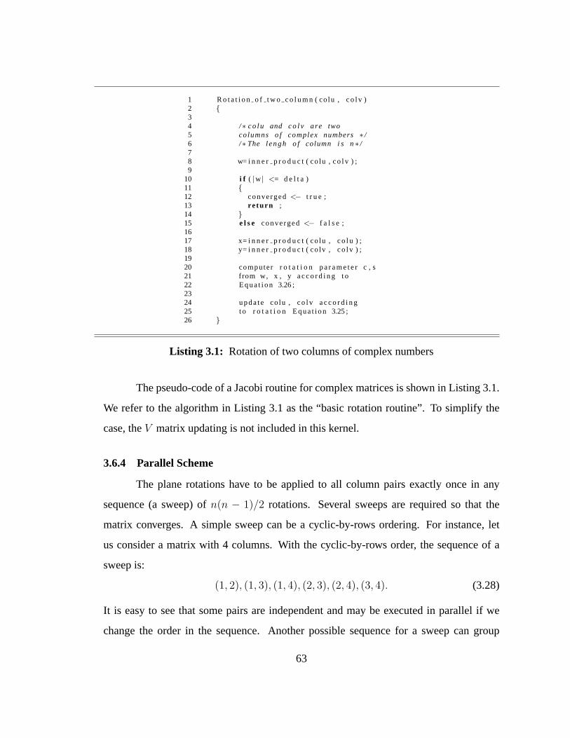
1 R o t a t i o n o f t w o c o l u m n ( co lu , co l v )2 {34 /∗ co lu and c o l v are two5 columns o f complex numbers∗ /6 /∗ The lengh o f column i s n∗ /78 w= i n n e r p r o d u c t ( co lu , co l v ) ;9

10 i f ( |w | <= d e l t a )11 {12 converged<− t r u e ;13 re turn ;14 }15 e l s e converged<− f a l s e ;1617 x= i n n e r p r o d u c t ( co lu , co lu ) ;18 y= i n n e r p r o d u c t ( co lv , co l v ) ;1920 computer r o t a t i o n p a r a m e t e r c , s21 from w, x , y a c c o r d i n g t o22 Equa t i on 3.26 ;2324 upda te co lu , co l v a c c o r d i n g25 t o r o t a t i o n Equa t i on 3.25 ;26 }

Listing 3.1: Rotation of two columns of complex numbers

The pseudo-code of a Jacobi routine for complex matrices is shown in Listing 3.1.

We refer to the algorithm in Listing 3.1 as the “basic rotation routine”. To simplify the

case, theV matrix updating is not included in this kernel.

3.6.4 Parallel Scheme

The plane rotations have to be applied to all column pairs exactly once in any

sequence (a sweep) ofn(n − 1)/2 rotations. Several sweeps are required so that the

matrix converges. A simple sweep can be a cyclic-by-rows ordering. For instance, let

us consider a matrix with 4 columns. With the cyclic-by-rowsorder, the sequence of a

sweep is:

(1, 2), (1, 3), (1, 4), (2, 3), (2, 4), (3, 4). (3.28)

It is easy to see that some pairs are independent and may be executed in parallel if we

change the order in the sequence. Another possible sequencefor a sweep can group

63

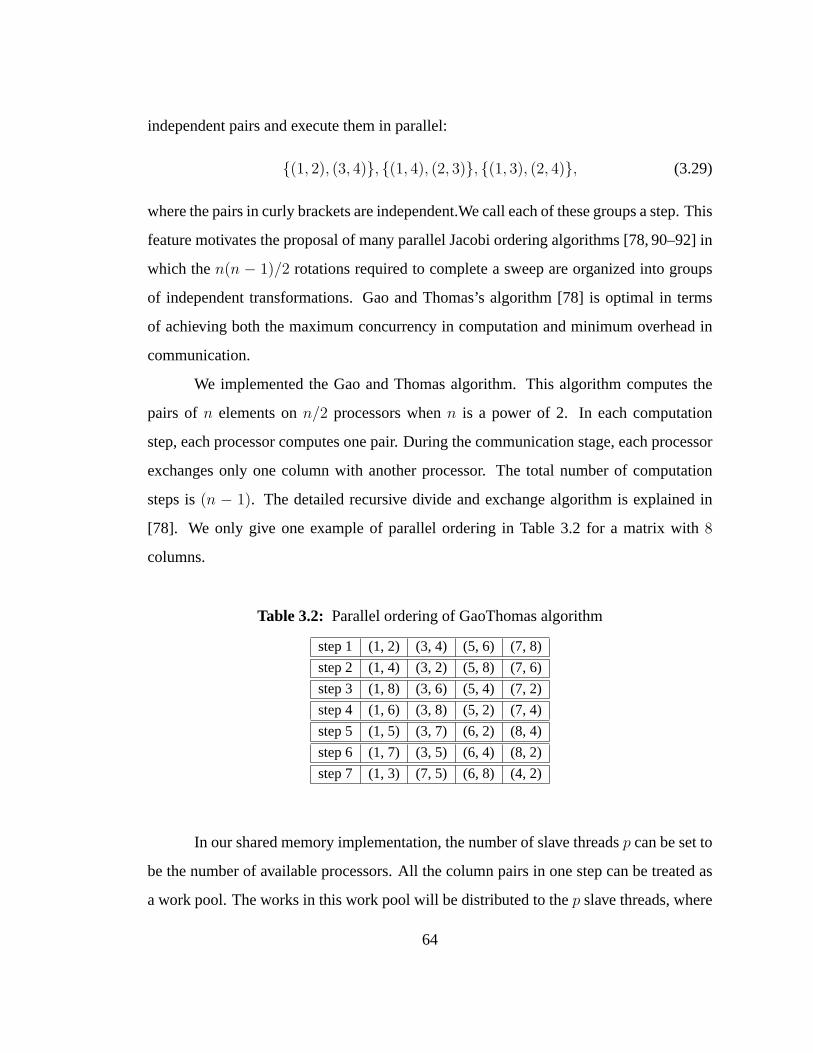
independent pairs and execute them in parallel:

{(1, 2), (3, 4)}, {(1, 4), (2, 3)}, {(1, 3), (2, 4)}, (3.29)

where the pairs in curly brackets are independent.We call each of these groups a step. This

feature motivates the proposal of many parallel Jacobi ordering algorithms [78, 90–92] in

which then(n − 1)/2 rotations required to complete a sweep are organized into groups

of independent transformations. Gao and Thomas’s algorithm [78] is optimal in terms

of achieving both the maximum concurrency in computation and minimum overhead in

communication.

We implemented the Gao and Thomas algorithm. This algorithmcomputes the

pairs ofn elements onn/2 processors whenn is a power of 2. In each computation

step, each processor computes one pair. During the communication stage, each processor

exchanges only one column with another processor. The totalnumber of computation

steps is(n − 1). The detailed recursive divide and exchange algorithm is explained in

[78]. We only give one example of parallel ordering in Table 3.2 for a matrix with8

columns.

Table 3.2: Parallel ordering of GaoThomas algorithm

step 1 (1, 2) (3, 4) (5, 6) (7, 8)

step 2 (1, 4) (3, 2) (5, 8) (7, 6)

step 3 (1, 8) (3, 6) (5, 4) (7, 2)

step 4 (1, 6) (3, 8) (5, 2) (7, 4)

step 5 (1, 5) (3, 7) (6, 2) (8, 4)

step 6 (1, 7) (3, 5) (6, 4) (8, 2)

step 7 (1, 3) (7, 5) (6, 8) (4, 2)

In our shared memory implementation, the number of slave threadsp can be set to

be the number of available processors. All the column pairs in one step can be treated as

a work pool. The works in this work pool will be distributed tothep slave threads, where

64

1 ≤ p ≤ n2. After each step, we implemented a barrier to make sure the stepk + 1 always

uses the updated column pairs from stepk. At the end of each sweep, we check whether

the convergence condition is satisfied. If not, we start a newsweep again. Otherwise, the

program terminates.

The convergence behavior of different orderings may not be the same. Hansen

[93] discusses the convergence properties associated withvarious ordering. In our imple-

mentation, we chose to use a threshold approach in order to enforce convergence [94].

We omit any rotation if the inner product(~u)H~v of the current column pairs~u and~v is

below a certain thresholdδ. Theδ is defined as :

δ = ǫ ·

N∑

i=1

A[i]HA[i], (3.30)

whereǫ is the machine precision epsilon andA[i] is theith column of the initialA matrix.

At the end of each sweep, if all the possible pairs in the sweephave converged according

to the above standard, then the problem has converged.

3.6.5 Group-based GaoThomas Algorithm

As stated previously, the GaoThomas algorithm can computen(n−1)/2 rotations

of a matrix withn columns onn/2 processors. When the size of the matrix increases,

group-based GaoThomas can be adopted. For instance, when the matrix size is2n and

we only haven/2 processors, we can group two columns together and treat themas one

single unit. Then the primary algorithm for a matrix withn columns can be used.

For a matrix withn columns, if we groupg columns together as a group, then we

haven/g groups and can use the basic GaoThomas algorithm forn/g elements, except

each element is a group. For instance, operations on a matrix16 by 16 can set the group

size to be 2, yielding 8 groups for which we can still use the divide and exchange algo-

rithm shown in Table 3.2. The only difference is that each bracket in the table is a rotation

of two groups, each group containing 2 columns in this case.

65

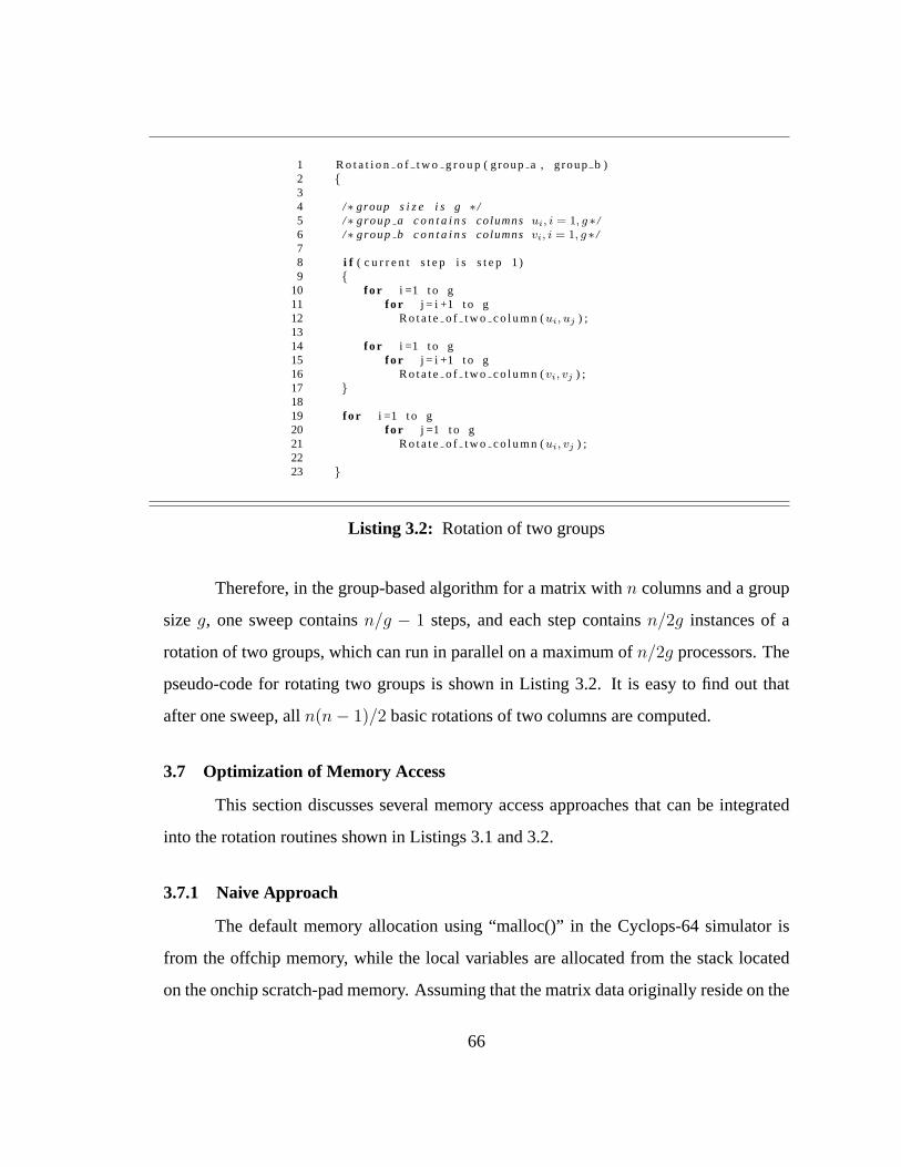
1 R o t a t i o n o f t w o g r o u p ( group a , g roup b )2 {34 /∗ group s i z e i s g ∗ /5 /∗ group a c o n t a i n s columnsui, i = 1, g ∗ /6 /∗ group b c o n t a i n s columnsvi, i = 1, g ∗ /78 i f ( c u r r e n t s t e p i s s t e p 1)9 {

10 f o r i =1 t o g11 f o r j = i +1 t o g12 R o t a t e o f t w o c o l u m n (ui, uj ) ;1314 f o r i =1 t o g15 f o r j = i +1 t o g16 R o t a t e o f t w o c o l u m n (vi, vj ) ;17 }1819 f o r i =1 t o g20 f o r j =1 t o g21 R o t a t e o f t w o c o l u m n (ui, vj ) ;2223 }

Listing 3.2: Rotation of two groups

Therefore, in the group-based algorithm for a matrix withn columns and a group

sizeg, one sweep containsn/g − 1 steps, and each step containsn/2g instances of a

rotation of two groups, which can run in parallel on a maximumof n/2g processors. The

pseudo-code for rotating two groups is shown in Listing 3.2.It is easy to find out that

after one sweep, alln(n − 1)/2 basic rotations of two columns are computed.

3.7 Optimization of Memory Access

This section discusses several memory access approaches that can be integrated

into the rotation routines shown in Listings 3.1 and 3.2.

3.7.1 Naive Approach

The default memory allocation using “malloc()” in the Cyclops-64 simulator is

from the offchip memory, while the local variables are allocated from the stack located

on the onchip scratch-pad memory. Assuming that the matrix data originally reside on the

66

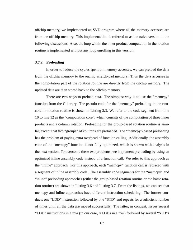
offchip memory, we implemented an SVD program where all the memory accesses are

from the offchip memory. This implementation is referred toas the naive version in the

following discussions. Also, the loop within the inner product computation in the rotation

routine is implemented without any loop unrolling in this version.

3.7.2 Preloading

In order to reduce the cycles spent on memory accesses, we canpreload the data

from the offchip memory to the onchip scratch-pad memory. Thus the data accesses in

the computation part of the rotation routine are directly from the onchip memory. The

updated data are then stored back to the offchip memory.

There are two ways to preload data. The simplest way is to use the “memcpy”

function from the C library. The pseudo-code for the “memcpy” preloading in the two-

column rotation routine is shown in Listing 3.3. We refer to the code segment from line

10 to line 12 as the “computation core”, which consists of thecomputation of three inner

products and a column rotation. Preloading for the group-based rotation routine is simi-

lar, except that two “groups” of columns are preloaded. The “memcpy”-based preloading

has the problem of paying extra overhead of function calling. Additionally, the assembly

code of the “memcpy” function is not fully optimized, which is shown with analysis in

the next section. To overcome these two problems, we implement preloading by using an

optimized inline assembly code instead of a function call. We refer to this approach as

the “inline” approach. For this approach, each “memcpy” function call is replaced with

a segment of inline assembly code. The assembly code segments for the “memcpy” and

“inline” preloading approaches (either the group-based rotation routine or the basic rota-

tion routine) are shown in Listing 3.6 and Listing 3.7. From the listings, we can see that

memcpy and inline approaches have different instruction scheduling. The former con-

ducts one “LDD” instruction followed by one “STD” and repeats for a sufficient number

of times until all the data are moved successfully. The latter, in contrast, issues several

“LDD” instructions in a row (in our case, 8 LDDs in a row) followed by several “STD”s

67

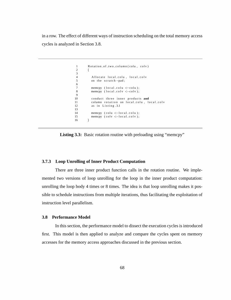
in a row. The effect of different ways of instruction scheduling on the total memory access

cycles is analyzed in Section 3.8.

1 R o t a t i o n o f t w o c o l u m n ( co lu , co l v )2 {34 A l l o c a t e l o c a l c o l u , l o c a l c o l v5 on t h e s c r a t c h−pad ;67 memcpy ( l o c a l c o l u <−co lu ) ;8 memcpy ( l o c a l c o l v <−co l v ) ;9

10 conduc t t h r e e i n n e r p r o d u c t sand11 column r o t a t i o n on l o c a lc o l u , l o c a l c o l v12 as i n L i s t i n g . 3.11314 memcpy ( co lu<− l o c a l c o l u ) ;15 memcpy ( co l v<− l o c a l c o l v ) ;16 }

Listing 3.3: Basic rotation routine with preloading using “memcpy”

3.7.3 Loop Unrolling of Inner Product Computation

There are three inner product function calls in the rotationroutine. We imple-

mented two versions of loop unrolling for the loop in the inner product computation:

unrolling the loop body 4 times or 8 times. The idea is that loop unrolling makes it pos-

sible to schedule instructions from multiple iterations, thus facilitating the exploitation of

instruction level parallelism.

3.8 Performance Model

In this section, the performance model to dissect the execution cycles is introduced

first. This model is then applied to analyze and compare the cycles spent on memory

accesses for the memory access approaches discussed in the previous section.

68

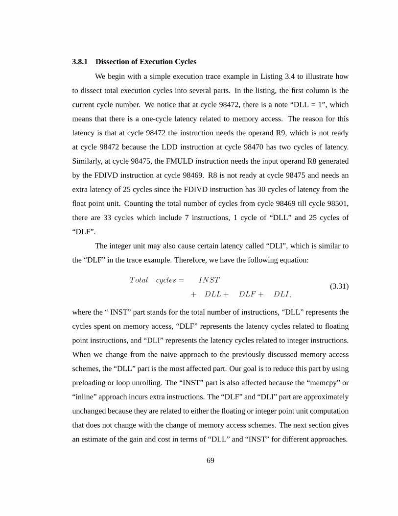
3.8.1 Dissection of Execution Cycles

We begin with a simple execution trace example in Listing 3.4to illustrate how

to dissect total execution cycles into several parts. In thelisting, the first column is the

current cycle number. We notice that at cycle 98472, there isa note “DLL = 1”, which

means that there is a one-cycle latency related to memory access. The reason for this

latency is that at cycle 98472 the instruction needs the operand R9, which is not ready

at cycle 98472 because the LDD instruction at cycle 98470 hastwo cycles of latency.

Similarly, at cycle 98475, the FMULD instruction needs the input operand R8 generated

by the FDIVD instruction at cycle 98469. R8 is not ready at cycle 98475 and needs an

extra latency of 25 cycles since the FDIVD instruction has 30cycles of latency from the

float point unit. Counting the total number of cycles from cycle 98469 till cycle 98501,

there are 33 cycles which include 7 instructions, 1 cycle of “DLL” and 25 cycles of

“DLF”.

The integer unit may also cause certain latency called “DLI”, which is similar to

the “DLF” in the trace example. Therefore, we have the following equation:

Total cycles = INST

+ DLL + DLF + DLI,(3.31)

where the “ INST” part stands for the total number of instructions, “DLL” represents the

cycles spent on memory access, “DLF” represents the latencycycles related to floating

point instructions, and “DLI” represents the latency cycles related to integer instructions.

When we change from the naive approach to the previously discussed memory access

schemes, the “DLL” part is the most affected part. Our goal isto reduce this part by using

preloading or loop unrolling. The “INST” part is also affected because the “memcpy” or

“inline” approach incurs extra instructions. The “DLF” and“DLI” part are approximately

unchanged because they are related to either the floating or integer point unit computation

that does not change with the change of memory access schemes. The next section gives

an estimate of the gain and cost in terms of “DLL” and “INST” for different approaches.

69

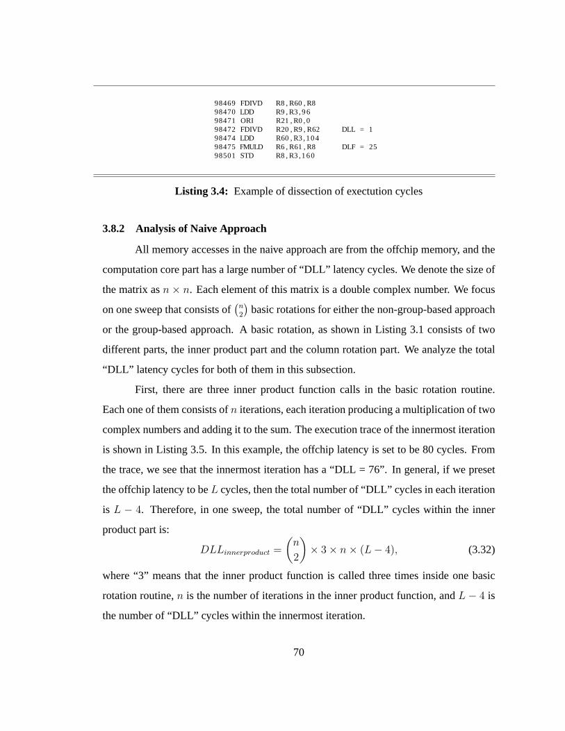
98469 FDIVD R8 , R60 , R898470 LDD R9 , R3 ,9698471 ORI R21 , R0 , 098472 FDIVD R20 , R9 , R62 DLL = 198474 LDD R60 , R3 ,10498475 FMULD R6 , R61 , R8 DLF = 2598501 STD R8 , R3 ,160

Listing 3.4: Example of dissection of exectution cycles

3.8.2 Analysis of Naive Approach

All memory accesses in the naive approach are from the offchip memory, and the

computation core part has a large number of “DLL” latency cycles. We denote the size of

the matrix asn × n. Each element of this matrix is a double complex number. We focus

on one sweep that consists of(

n2

)

basic rotations for either the non-group-based approach

or the group-based approach. A basic rotation, as shown in Listing 3.1 consists of two

different parts, the inner product part and the column rotation part. We analyze the total

“DLL” latency cycles for both of them in this subsection.

First, there are three inner product function calls in the basic rotation routine.

Each one of them consists ofn iterations, each iteration producing a multiplication of two

complex numbers and adding it to the sum. The execution traceof the innermost iteration

is shown in Listing 3.5. In this example, the offchip latencyis set to be 80 cycles. From

the trace, we see that the innermost iteration has a “DLL = 76”. In general, if we preset

the offchip latency to beL cycles, then the total number of “DLL” cycles in each iteration

is L − 4. Therefore, in one sweep, the total number of “DLL” cycles within the inner

product part is:

DLLinnerproduct =

(

n

2

)

× 3 × n × (L − 4), (3.32)

where “3” means that the inner product function is called three times inside one basic

rotation routine,n is the number of iterations in the inner product function, and L − 4 is

the number of “DLL” cycles within the innermost iteration.

70

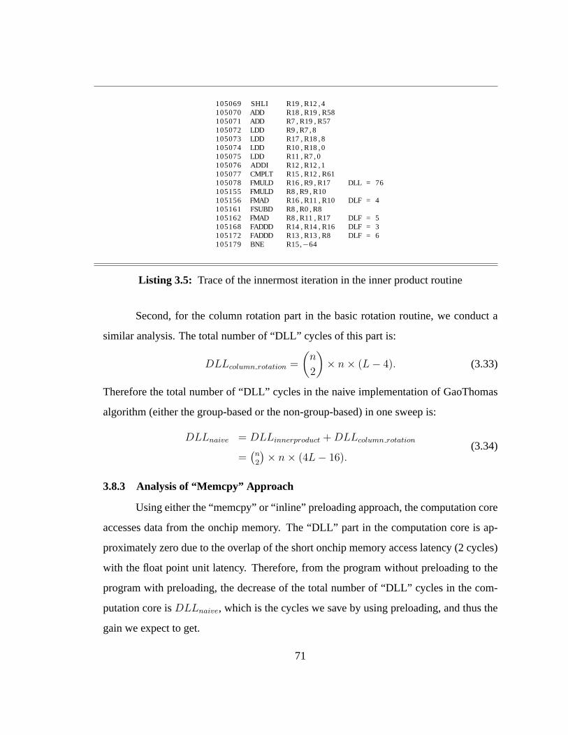
105069 SHLI R19 , R12 , 4105070 ADD R18 , R19 , R58105071 ADD R7 , R19 , R57105072 LDD R9 , R7 , 8105073 LDD R17 , R18 , 8105074 LDD R10 , R18 , 0105075 LDD R11 , R7 , 0105076 ADDI R12 , R12 , 1105077 CMPLT R15 , R12 , R61105078 FMULD R16 , R9 , R17 DLL = 76105155 FMULD R8 , R9 , R10105156 FMAD R16 , R11 , R10 DLF = 4105161 FSUBD R8 , R0 , R8105162 FMAD R8 , R11 , R17 DLF = 5105168 FADDD R14 , R14 , R16 DLF = 3105172 FADDD R13 , R13 , R8 DLF = 6105179 BNE R15,−64

Listing 3.5: Trace of the innermost iteration in the inner product routine

Second, for the column rotation part in the basic rotation routine, we conduct a

similar analysis. The total number of “DLL” cycles of this part is:

DLLcolumn rotation =

(

n

2

)

× n × (L − 4). (3.33)

Therefore the total number of “DLL” cycles in the naive implementation of GaoThomas

algorithm (either the group-based or the non-group-based)in one sweep is:

DLLnaive = DLLinnerproduct + DLLcolumn rotation

=(

n2

)

× n × (4L − 16).(3.34)

3.8.3 Analysis of “Memcpy” Approach

Using either the “memcpy” or “inline” preloading approach,the computation core

accesses data from the onchip memory. The “DLL” part in the computation core is ap-

proximately zero due to the overlap of the short onchip memory access latency (2 cycles)

with the float point unit latency. Therefore, from the program without preloading to the

program with preloading, the decrease of the total number of“DLL” cycles in the com-

putation core isDLLnaive, which is the cycles we save by using preloading, and thus the

gain we expect to get.

71

Moving data from the offchip memory to the onchip memory results in an extra

cost, which consists of two parts: the first part is the total “DLL” cycles in the code

segment that is responsible for moving data, and the second part is the extra instructions

incurred.

Firstly, we derive the total number of “memcpy” function calls (which are respon-

sible for loading data “in”). For the basic non-group-basedGaoThomas algorithm, there

is a total of(

n2

)

basic rotations (shown in Listing 3.1) in one sweep. A basic rotation needs

to load in two columns, each of lengthn. Loading a double complex number needs two

“LDD” instructions. Therefore, the total number of “LDD”s for preloading data is:

LDDmemcpy no group =(

n2

)

× 2 × n × 2

=(

n2

)

× 4n,(3.35)

where the first “2” stands for loading “two” columns,n is the length of the column, and

the second “2” means that loading a double complex number needs two LDDs.

For the group-based algorithm, if the group size isg, there is a total of(

n/g2

)

group-

based rotations. At the beginning of each group-based rotation, we need to load in two

groups of columns (i.e,2 × g columns) and each column needsn × 2 LDDs. Therefore,

the total number of LDDs for preloading data during one sweepis:

LDDmemcpy =(

n/g2

)

× 2g × n × 2

=(

n/g2

)

× g × 4n.(3.36)

If we treat the non-group-based GaoThomas algorithm as a group-based algorithm

with group size one, then we can use (3.36) for either the group-based algorithm or non-

group-based algorithm.

Secondly, we compute the latency incurred by the LDDs. The execution trace

segment of the assembly code for the “memcpy” function is shown in Listing 3.6, with

the offchip latency set to be 80. From Listing 3.6, we observethat each LDD instruction

causes a long latency of 80 cycles. This latency is reflected where the “STD” instructions

72

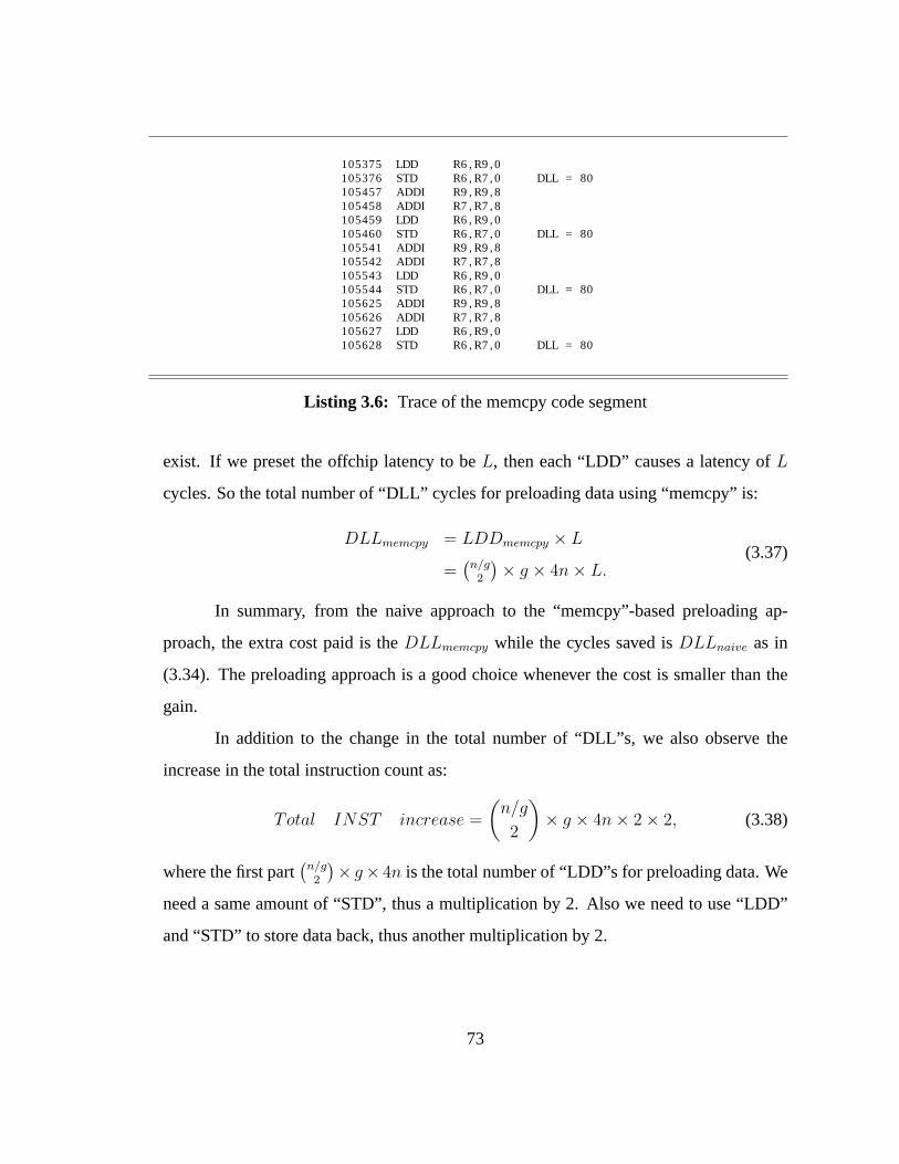
105375 LDD R6 , R9 , 0105376 STD R6 , R7 , 0 DLL = 80105457 ADDI R9 , R9 , 8105458 ADDI R7 , R7 , 8105459 LDD R6 , R9 , 0105460 STD R6 , R7 , 0 DLL = 80105541 ADDI R9 , R9 , 8105542 ADDI R7 , R7 , 8105543 LDD R6 , R9 , 0105544 STD R6 , R7 , 0 DLL = 80105625 ADDI R9 , R9 , 8105626 ADDI R7 , R7 , 8105627 LDD R6 , R9 , 0105628 STD R6 , R7 , 0 DLL = 80

Listing 3.6: Trace of the memcpy code segment

exist. If we preset the offchip latency to beL, then each “LDD” causes a latency ofL

cycles. So the total number of “DLL” cycles for preloading data using “memcpy” is:

DLLmemcpy = LDDmemcpy × L

=(

n/g2

)

× g × 4n × L.(3.37)

In summary, from the naive approach to the “memcpy”-based preloading ap-

proach, the extra cost paid is theDLLmemcpy while the cycles saved isDLLnaive as in

(3.34). The preloading approach is a good choice whenever the cost is smaller than the

gain.

In addition to the change in the total number of “DLL”s, we also observe the

increase in the total instruction count as:

Total INST increase =

(

n/g

2

)

× g × 4n × 2 × 2, (3.38)

where the first part(

n/g2

)

× g× 4n is the total number of “LDD”s for preloading data. We

need a same amount of “STD”, thus a multiplication by 2. Also we need to use “LDD”

and “STD” to store data back, thus another multiplication by2.

73

3.8.4 Analysis of “Inline” Approach

The total amount of data preloaded for the “inline” preloading approach is the

same as the “memcpy” approach. Therefore, the total number of “LDD”s of the inline

approach is the same as the “memcpy” approach:

LDDinline =(

n/g2

)

× 2g × n × 2

=(

n/g2

)

× g × 4n,(3.39)

wheren is the matrix size andg is the group size..

The difference between the “inline” approach and “memcpy” approach is the

scheduling of the LDD and STD instructions in the assembly code. As shown in List-

ing 3.6, each LDD in the “memcpy” approach is followed immediately by one STD. In

the “inline” approach, 8 LDDs in a row are followed by 8 STDs ina row, as shown in

Listing 3.7. From the trace we can see that we will have one “DLL=73” every 8 LDDs

if we preset the offchip latency to be 80. If the offchip latency is L cycles, there is a

“DLL= L − 7” every 8 “LDD” instructions. Therefore, the total number of“DLL” cycles

for preloading data using the “inline” approach is:

DLLinline = LDDinline/8 × (L − 7)

= 18×

(

n/g2

)

× g × 4n × (L − 7).(3.40)

From (3.40), we can see very clearly that preloading data using the “inline” approach

is better than using the “memcpy” approach becauseDLLinline is approximately1/8 of

DLLmemcpy.

From the naive approach to the “inline” preloading approach, the extra cost paid

is theDLLinline, while the cycles saved isDLLnaive as in (3.34). Increase in the total

instruction count is computed according to (3.38). It is also noteworthy that the “inline”

approach should have a smaller instruction count increase than the “memcpy” approach

since the former does not need the instructions involved in function calling.

74

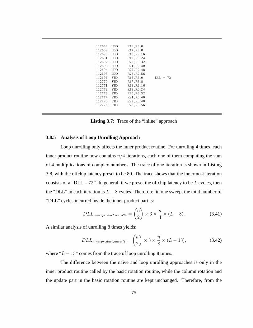
112688 LDD R16 , R9 , 0112689 LDD R17 , R9 , 8112690 LDD R18 , R9 ,16112691 LDD R19 , R9 ,24112692 LDD R20 , R9 ,32112693 LDD R21 , R9 ,40112694 LDD R22 , R9 ,48112695 LDD R28 , R9 ,56112696 STD R16 , R6 , 0 DLL = 73112770 STD R17 , R6 , 8112771 STD R18 , R6 ,16112772 STD R19 , R6 ,24112773 STD R20 , R6 ,32112774 STD R21 , R6 ,40112775 STD R22 , R6 ,48112776 STD R28 , R6 ,56

Listing 3.7: Trace of the “inline” approach

3.8.5 Analysis of Loop Unrolling Approach

Loop unrolling only affects the inner product routine. For unrolling 4 times, each

inner product routine now containsn/4 iterations, each one of them computing the sum

of 4 multiplications of complex numbers. The trace of one iteration is shown in Listing

3.8, with the offchip latency preset to be 80. The trace showsthat the innermost iteration

consists of a “DLL = 72”. In general, if we preset the offchip latency to beL cycles, then

the “DLL” in each iteration isL− 8 cycles. Therefore, in one sweep, the total number of

“DLL” cycles incurred inside the inner product part is:

DLLinnerproduct unroll4 =

(

n

2

)

× 3 ×n

4× (L − 8). (3.41)

A similar analysis of unrolling 8 times yields:

DLLinnerproduct unroll8 =

(

n

2

)

× 3 ×n

8× (L − 13), (3.42)

where “L − 13” comes from the trace of loop unrolling 8 times.

The difference between the naive and loop unrolling approaches is only in the

inner product routine called by the basic rotation routine,while the column rotation and

the update part in the basic rotation routine are kept unchanged. Therefore, from the

75

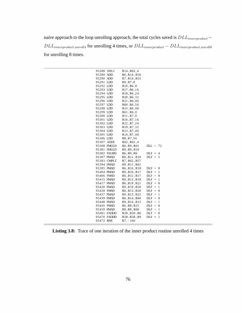
naive approach to the loop unrolling approach, the total cycles saved isDLLinnerproduct−

DLLinnerproduct unroll4 for unrolling 4 times, orDLLinnerproduct − DLLinnerproduct unroll8

for unrolling 8 times.

95288 SHLI R14 , R62 , 495289 ADD R6 , R14 , R5695290 ADD R7 , R14 , R5595291 LDD R9 , R7 , 895292 LDD R10 , R6 , 895293 LDD R17 , R6 ,1695294 LDD R18 , R6 ,2495295 LDD R20 , R6 ,3295296 LDD R21 , R6 ,4095297 LDD R60 , R6 ,5695298 LDD R15 , R6 ,4895299 LDD R61 , R6 , 095300 LDD R11 , R7 , 095301 LDD R16 , R7 ,1695302 LDD R12 , R7 ,2495303 LDD R19 , R7 ,3295304 LDD R13 , R7 ,4095305 LDD R14 , R7 ,4895306 LDD R8 , R7 ,5695307 ADDI R62 , R62 , 495308 FMULD R6 , R9 , R61 DLL = 7295381 FMULD R9 , R9 , R1095382 FSUBD R6 , R0 , R6 DLF = 495387 FMAD R6 , R11 , R10 DLF = 595393 CMPLT R7 , R62 , R5795394 FMAD R9 , R11 , R6195395 FMAD R6 , R16 , R18 DLF = 895404 FMAD R9 , R16 , R17 DLF = 195406 FMSD R6 , R12 , R17 DLF = 895415 FMAD R9 , R12 , R18 DLF = 195417 FMAD R6 , R19 , R21 DLF = 895426 FMAD R9 , R19 , R20 DLF = 195428 FMSD R6 , R13 , R20 DLF = 895437 FMAD R9 , R13 , R21 DLF = 195439 FMAD R6 , R14 , R60 DLF = 895448 FMAD R9 , R14 , R15 DLF = 195450 FMSD R6 , R8 , R15 DLF = 895459 FMAD R9 , R8 , R60 DLF = 195461 FADDD R59 , R59 , R6 DLF = 895470 FADDD R58 , R58 , R9 DLF = 195472 BNE R7,−160

Listing 3.8: Trace of one iteration of the inner product routine unrolled4 times

76

3.9 Experimental Results

In this section, we present experimental results: the speedup of the loop level

parallelization and the fine level parallelization of SVD, as well as the comparison of

different memory access schemes.

3.9.1 Target Platform and Simulation Environment

Our test platforms include a Sunfire SMP machine from Sun Inc., a Linux cluster

and a cellular computer architecture Cyclops-64.

The software tool chain of the Cyclops-64 platform currentlyprovides a compiler,

linker and simulator for users. A number of optimization levels are supported by the

compiler. A functional accurate simulator (FAST) is also provided. The main features

are: (1) the simulator supports most of the features of Cyclops-64 architecture, including

multithreaded execution, Cyclops-64 ISA, floating point unit, interrupts, memory mapped

features (interthread interrupt and wakeup signal); (2) FAST can generate the execution

trace and/or an instruction statistics report to help a software/application developer tuning

and optimizing a program. Furthermore, the macros “Trace On” and “Trace off” allow

us to generate trace for a specific segment of code and save thetrace to a file; (3) It can

also generate a timing result at the cycle level of a program.For an application to be

simulated, the code must be slightly modified. The Cyclops-64software tool chain runs

on Linux environment.

We also developed a Trace Analyzer that can take the output trace from the simu-

lator and generate the dissection of execution cycles and analysis of the code simulated.

The trace analyzer can generate the following statistics: (1) the dissection of the execution

cycles to the four different parts, as shown in (3.31); (2) the analyzer can also generate sta-

tistics about the total “DLL” related to a certain instruction. For instance, in the example

shown in Listing 3.7, the “DLL” latencies caused by the “LDD”instruction are reflected

in the STD instruction. We call such latencies “associated”with the STD instruction. The

analyzer can sum the total “DLL”s associated with the STD instruction. The sum is the

77

total memory access cycles in the code segment of data preloading, as in (3.37) or (3.40).

Similarly, the “DLL”s associated with the float point instructions such as “FMULD” or

“FMAD” are the “DLL”s in the computation core, as in (3.34).

3.9.2 Loop Level Parallelization

The loop level parallelization is carried out on a Sunfire SMPmachine and a Linux

cluster. The SMP machine used is the DBI-RNA1 at the Delaware Biotechnology Insti-

tute. DBI-RNA1 is a Sun Sunfire 4800 Server with 12 SPARC 750MHz CPUs, and a 24

gigabyte memory. The code has also been ported to the Cellularcomputer architecture

Cyclops-64. However, due to the fact that the Simulator at this stage is slow to carry out

the loop level parallelization experiment, we only presentthe Loop level parallelization

result on a Sunfire SMP machine and a Linux cluster.

In the data used in this experiment, the number of coils is 4, the image size is 128

by 128 and the number of phase encodes is 38.

Fig. 3.10 presents the result of both Pthread and OpenMP. Thespeedup of both

the total execution time and the loop only are presented. From the figure, it is seen that

both Pthread and OpenMP achieved near linear performance upto 12 threads. This is due

to the fact that the tasks (iterations) of the loop are totally independent of each other.

According to the well known “Amdahl’s” law, if a program can be expressed as

two portions, the serial portion S and the parallel portion P, then the timeT (n) required

to complete a task onn parallel processors is:

T (n) = S +P

n, (3.43)

and the speedup for n CPUs can be expressed as:

sp =T (1)

T (n)=

S + P

S + Pn

. (3.44)

78

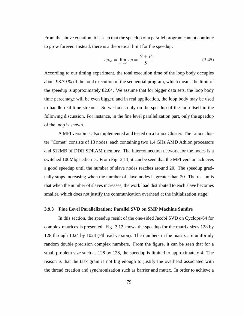
From the above equation, it is seen that the speedup of a parallel program cannot continue

to grow forever. Instead, there is a theoretical limit for the speedup:

sp∞ = limn→∞

sp =S + P

S. (3.45)

According to our timing experiment, the total execution time of the loop body occupies

about 98.79 % of the total execution of the sequential program, which means the limit of

the speedup is approximately 82.64. We assume that for bigger data sets, the loop body

time percentage will be even bigger, and in real application, the loop body may be used

to handle real-time streams. So we focus only on the speedup of the loop itself in the

following discussion. For instance, in the fine level parallelization part, only the speedup

of the loop is shown.

A MPI version is also implemented and tested on a Linux Cluster. The Linux clus-

ter “Comet” consists of 18 nodes, each containing two 1.4 GHz AMD Athlon processors

and 512MB of DDR SDRAM memory. The interconnection network for the nodes is a

switched 100Mbps ethernet. From Fig. 3.11, it can be seen that the MPI version achieves

a good speedup until the number of slave nodes reaches around20. The speedup grad-

ually stops increasing when the number of slave nodes is greater than 20. The reason is

that when the number of slaves increases, the work load distributed to each slave becomes

smaller, which does not justify the communication overheadat the initialization stage.

3.9.3 Fine Level Parallelization: Parallel SVD on SMP Machine Sunfire

In this section, the speedup result of the one-sided Jacobi SVD on Cyclops-64 for

complex matrices is presented. Fig. 3.12 shows the speedup for the matrix sizes 128 by

128 through 1024 by 1024 (Pthread version). The numbers in the matrix are uniformly

random double precision complex numbers. From the figure, itcan be seen that for a

small problem size such as 128 by 128, the speedup is limited to approximately 4. The

reason is that the task grain is not big enough to justify the overhead associated with

the thread creation and synchronization such as barrier andmutex. In order to achieve a

79

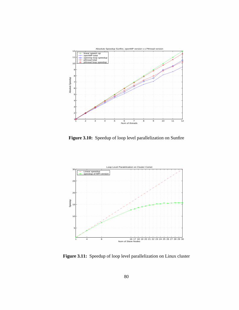
1 2 3 4 5 6 7 8 9 10 11 121

2

3

4

5

6

7

8

9

10

11

12

Num of threads

Abso

lute

Spe

edup

Absolute Speedup Sunfire, openMP version v.s Pthread version

linear speed−upopenMP totalopenmp loop speeduppthread totalpthread loop speedup

Figure 3.10: Speedup of loop level parallelization on Sunfire

1 4 8 16 17 18 19 20 21 22 23 24 25 26 27 28 29 30

5

10

15

20

25

30

Num of Slave Nodes

Spee

dup

Loop Level Paralelization on Cluster Comet

Linear speedupspeedup of MPI version

Figure 3.11: Speedup of loop level parallelization on Linux cluster

80

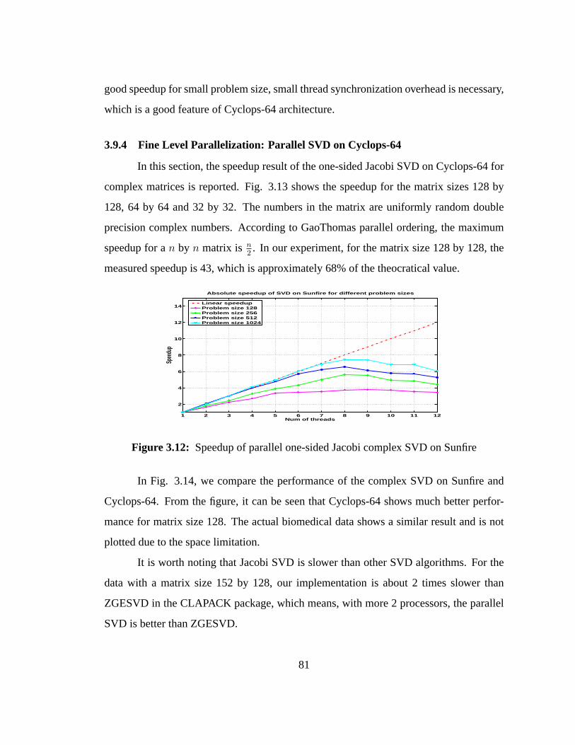
good speedup for small problem size, small thread synchronization overhead is necessary,

which is a good feature of Cyclops-64 architecture.

3.9.4 Fine Level Parallelization: Parallel SVD on Cyclops-64

In this section, the speedup result of the one-sided Jacobi SVD on Cyclops-64 for

complex matrices is reported. Fig. 3.13 shows the speedup for the matrix sizes 128 by

128, 64 by 64 and 32 by 32. The numbers in the matrix are uniformly random double

precision complex numbers. According to GaoThomas parallel ordering, the maximum

speedup for an by n matrix is n2. In our experiment, for the matrix size 128 by 128, the

measured speedup is 43, which is approximately 68% of the theocratical value.

1 2 3 4 5 6 7 8 9 10 11 12

2

4

6

8

10

12

14

Num of threads

Spee

dup

Absolute speedup of SVD on Sunfire for different problem sizes

Linear speedupProblem size 128Problem size 256Problem size 512Problem size 1024

Figure 3.12: Speedup of parallel one-sided Jacobi complex SVD on Sunfire

In Fig. 3.14, we compare the performance of the complex SVD onSunfire and

Cyclops-64. From the figure, it can be seen that Cyclops-64 shows much better perfor-

mance for matrix size 128. The actual biomedical data shows asimilar result and is not

plotted due to the space limitation.

It is worth noting that Jacobi SVD is slower than other SVD algorithms. For the

data with a matrix size 152 by 128, our implementation is about 2 times slower than

ZGESVD in the CLAPACK package, which means, with more 2 processors, the parallel

SVD is better than ZGESVD.

81

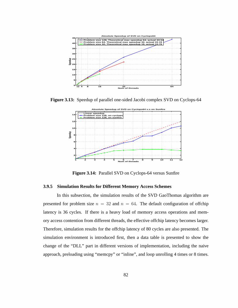
12 4 8 16 32 640

5

10

15

20

25

30

35

40

45

Num of threads

Spee

dup

Absolute Speedup of SVD on Cyclops64

Problem size 128, Theoretical max speedup 64, actual 43.54Problem size 64, Theoretical max speedup 32, actual 22.15Problem size 32, Theoretical max speedup 16, actual 10.76

Figure 3.13: Speedup of parallel one-sided Jacobi complex SVD on Cyclops-64

1 2 3 4 5 6 7 8 9 10 11 12

2

4

6

8

10

12

14

Num of threads

Spee

dup

Absolute Speedup of SVD on Cyclops64 v.s on Sunfire

Linear speedupProblem size 128, on cyclopsProblem size 128, on sunfire

Figure 3.14: Parallel SVD on Cyclops-64 versus Sunfire

3.9.5 Simulation Results for Different Memory Access Schemes

In this subsection, the simulation results of the SVD GaoThomas algorithm are

presented for problem sizen = 32 andn = 64. The default configuration of offchip

latency is 36 cycles. If there is a heavy load of memory accessoperations and mem-

ory access contention from different threads, the effective offchip latency becomes larger.

Therefore, simulation results for the offchip latency of 80cycles are also presented. The

simulation environment is introduced first, then a data table is presented to show the

change of the “DLL” part in different versions of implementation, including the naive

approach, preloading using “memcpy” or “inline”, and loop unrolling 4 times or 8 times.

82

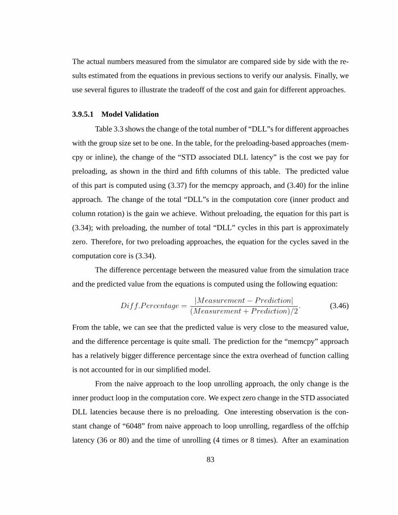
The actual numbers measured from the simulator are comparedside by side with the re-

sults estimated from the equations in previous sections to verify our analysis. Finally, we

use several figures to illustrate the tradeoff of the cost andgain for different approaches.

3.9.5.1 Model Validation

Table 3.3 shows the change of the total number of “DLL”s for different approaches

with the group size set to be one. In the table, for the preloading-based approaches (mem-

cpy or inline), the change of the “STD associated DLL latency” is the cost we pay for

preloading, as shown in the third and fifth columns of this table. The predicted value

of this part is computed using (3.37) for the memcpy approach, and (3.40) for the inline

approach. The change of the total “DLL”s in the computation core (inner product and

column rotation) is the gain we achieve. Without preloading, the equation for this part is

(3.34); with preloading, the number of total “DLL” cycles inthis part is approximately

zero. Therefore, for two preloading approaches, the equation for the cycles saved in the

computation core is (3.34).

The difference percentage between the measured value from the simulation trace

and the predicted value from the equations is computed usingthe following equation:

Diff.Percentage =|Measurement − Prediction|

(Measurement + Prediction)/2. (3.46)

From the table, we can see that the predicted value is very close to the measured value,

and the difference percentage is quite small. The prediction for the “memcpy” approach

has a relatively bigger difference percentage since the extra overhead of function calling

is not accounted for in our simplified model.

From the naive approach to the loop unrolling approach, the only change is the

inner product loop in the computation core. We expect zero change in the STD associated

DLL latencies because there is no preloading. One interesting observation is the con-

stant change of “6048” from naive approach to loop unrolling, regardless of the offchip

latency (36 or 80) and the time of unrolling (4 times or 8 times). After an examination

83

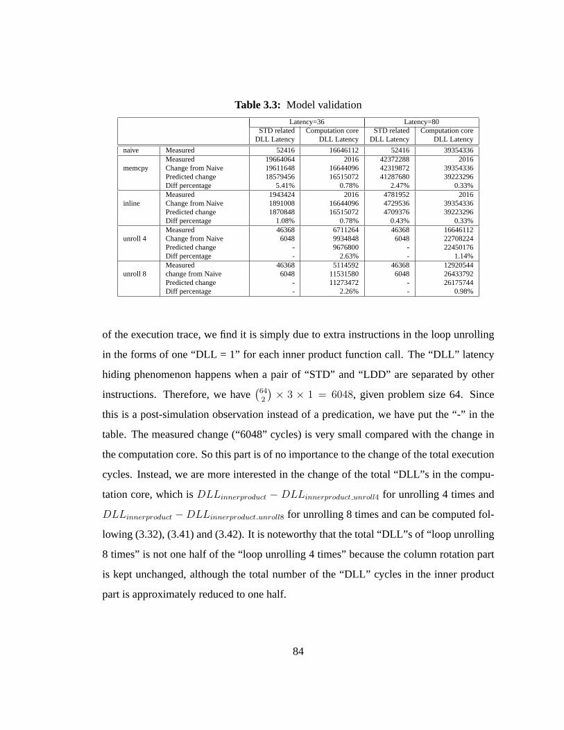
Table 3.3: Model validation

Latency=36 Latency=80STD related Computation core STD related Computation core

DLL Latency DLL Latency DLL Latency DLL Latency

naive Measured 52416 16646112 52416 39354336Measured 19664064 2016 42372288 2016

memcpy Change from Naive 19611648 16644096 42319872 39354336Predicted change 18579456 16515072 41287680 39223296Diff percentage 5.41% 0.78% 2.47% 0.33%Measured 1943424 2016 4781952 2016

inline Change from Naive 1891008 16644096 4729536 39354336Predicted change 1870848 16515072 4709376 39223296Diff percentage 1.08% 0.78% 0.43% 0.33%Measured 46368 6711264 46368 16646112

unroll 4 Change from Naive 6048 9934848 6048 22708224Predicted change - 9676800 - 22450176Diff percentage - 2.63% - 1.14%Measured 46368 5114592 46368 12920544

unroll 8 change from Naive 6048 11531580 6048 26433792Predicted change - 11273472 - 26175744Diff percentage - 2.26% - 0.98%

of the execution trace, we find it is simply due to extra instructions in the loop unrolling

in the forms of one “DLL = 1” for each inner product function call. The “DLL” latency

hiding phenomenon happens when a pair of “STD” and “LDD” are separated by other

instructions. Therefore, we have(

642

)

× 3 × 1 = 6048, given problem size 64. Since

this is a post-simulation observation instead of a predication, we have put the “-” in the

table. The measured change (“6048” cycles) is very small compared with the change in

the computation core. So this part is of no importance to the change of the total execution

cycles. Instead, we are more interested in the change of the total “DLL”s in the compu-

tation core, which isDLLinnerproduct − DLLinnerproduct unroll4 for unrolling 4 times and

DLLinnerproduct − DLLinnerproduct unroll8 for unrolling 8 times and can be computed fol-

lowing (3.32), (3.41) and (3.42). It is noteworthy that the total “DLL”s of “loop unrolling

8 times” is not one half of the “loop unrolling 4 times” because the column rotation part

is kept unchanged, although the total number of the “DLL” cycles in the inner product

part is approximately reduced to one half.

84

3.9.5.2 Comparison of Different Approaches

Fig. 3.15 illustrates the comparison of the five approaches by decomposing total

execution cycles into four parts as in (3.31). Each figure consists of five clusters of stacked

bars. The first cluster shows the results of five approaches with group size one, the second

one shows results for group size 2, and so on and so forth. Within each cluster, the leftmost

stacked bar illustrates the four-part dissection for the naive approach, the second and third

one depict the dissection for loop unrolling four times and eight times, and the fourth and

the fifth represent the “memcpy” and the “inline” preloadingapproaches. Within each

stacked bar, the brown bar (at the top), the deep blue bar (at the bottom), the light blue bar

and the yellow bar (in the middle) represent the “DLL” part, the number of instructions,

the “DLI” and the “DLF” part, respectively. The “DLI” part cannot be actually seen at

the current scale since it is very small compared to the otherparts.

We can see from the figure that the measurement matches the previous perfor-

mance analysis. Firstly, all the proposed approaches except the “memcpy” approach

achieve better performance – less execution cycles – than the naive approach. The “mem-

cpy” approach performs worse than the naive approach because its scheduling of “LDD”

and “STD” instructions results inL latency cycles for each “LDD/STD” pair in the data

preloading section. The “inline” approach, in contrast, has a better scheduling in which

every 8 “STD”s only incurL−7 latency cycles. Therefore, the “DLL” part of the “inline”

approach is approximately one eighth of that of the “memcpy”approach.

Secondly, the way that the “DLL” part changes with the increase of the group size

also confirms our analysis. For the preloading-based approaches (either “memcpy” or

“inline”), the “DLL” part reduces to approximately one halfwhen the group size doubles,

which coincides with the predictions of (3.37) and (3.40). The “memcpy” approach has

a large value for the “DLL” part when the group size equals one; thus its “DLL” part

decreases significantly from group size one to two and becomes smaller than that of the

naive approach when the group size reaches three. On the contrary, the “DLL” part of

85

the loop unrolling-based approach does not change with the change of the group size, as

indicated by (3.41) and (3.42).

Thirdly, from the naive approach to the other four approaches, the increase or de-

crease of the number of total instructions (the bottom bar inthe stacked bar) also matches

our expectation. The extra overhead for data preloading constitutes the increase of this

part for the preloading-based approaches, which can be estimated according to (3.38).

The “memcpy” approach has more instructions than the “inline” approach because func-

tion calls incur extra instructions. On the other hand, the loop unrolling approach reduces

the total instruction cycles from the naive approach since it has a smaller number of times

that the loop control statement gets executed.

Fourthly, the “DLF” part in the figures approximately does not change no matter

which approaches we use. This is due to the fact that it represents the latencies related to

the floating point instructions that are kept unchanged. However, the figures do show a mi-

nor increase of “DLF” from the naive approach to the preloading-based approaches. The

reason is explained as follows. A code segment often includes both floating point opera-

tions and memory access operations; thus the “DLL” part and the “DLF” part sometimes

overlap with each other. Without preloading, the memory accesses in the computation

core have a long latency, thus the “DLF”s that overlap with “DLL”s get hidden by long

“DLL”s. With preloading, the memory operations are mainly from onchip memory and

the access latency becomes short; thus those “DLF”s can no longer be hidden by “DLL”s

and become explicit. Nonetheless, the change of the “DLF” part is very small compared

to the change of the “DLL” part and thus can be omitted safely.

Lastly, we can see that the “inline” preloading approach performs the best out of

all five approaches. In fact, from the naive approach to the “inline” approach, the number

of total execution cycles is reduced by 52% for latency 80, and 43% for latency 36 (with

the problem size 64 by 64 and the group size 1).

86

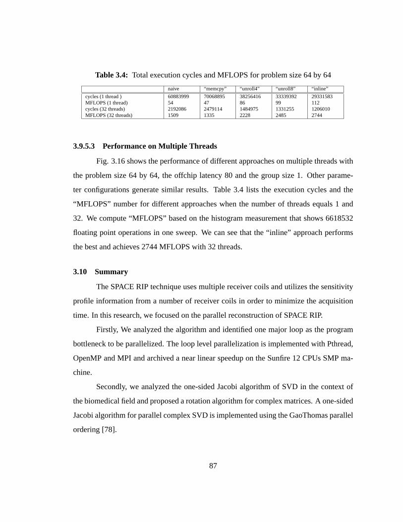
Table 3.4: Total execution cycles and MFLOPS for problem size 64 by 64

naive “memcpy” “unroll4” “unroll8” “inline”

cycles (1 thread ) 60883999 70068895 38256416 33339392 29331583MFLOPS (1 thread) 54 47 86 99 112cycles (32 threads) 2192086 2479114 1484975 1331255 1206010MFLOPS (32 threads) 1509 1335 2228 2485 2744

3.9.5.3 Performance on Multiple Threads

Fig. 3.16 shows the performance of different approaches on multiple threads with

the problem size 64 by 64, the offchip latency 80 and the groupsize 1. Other parame-

ter configurations generate similar results. Table 3.4 lists the execution cycles and the

“MFLOPS” number for different approaches when the number ofthreads equals 1 and

32. We compute “MFLOPS” based on the histogram measurement that shows 6618532

floating point operations in one sweep. We can see that the “inline” approach performs

the best and achieves 2744 MFLOPS with 32 threads.

3.10 Summary

The SPACE RIP technique uses multiple receiver coils and utilizes the sensitivity

profile information from a number of receiver coils in order to minimize the acquisition

time. In this research, we focused on the parallel reconstruction of SPACE RIP.

Firstly, We analyzed the algorithm and identified one major loop as the program

bottleneck to be parallelized. The loop level parallelization is implemented with Pthread,

OpenMP and MPI and archived a near linear speedup on the Sunfire 12 CPUs SMP ma-

chine.

Secondly, we analyzed the one-sided Jacobi algorithm of SVDin the context of

the biomedical field and proposed a rotation algorithm for complex matrices. A one-sided

Jacobi algorithm for parallel complex SVD is implemented using the GaoThomas parallel

ordering [78].

87

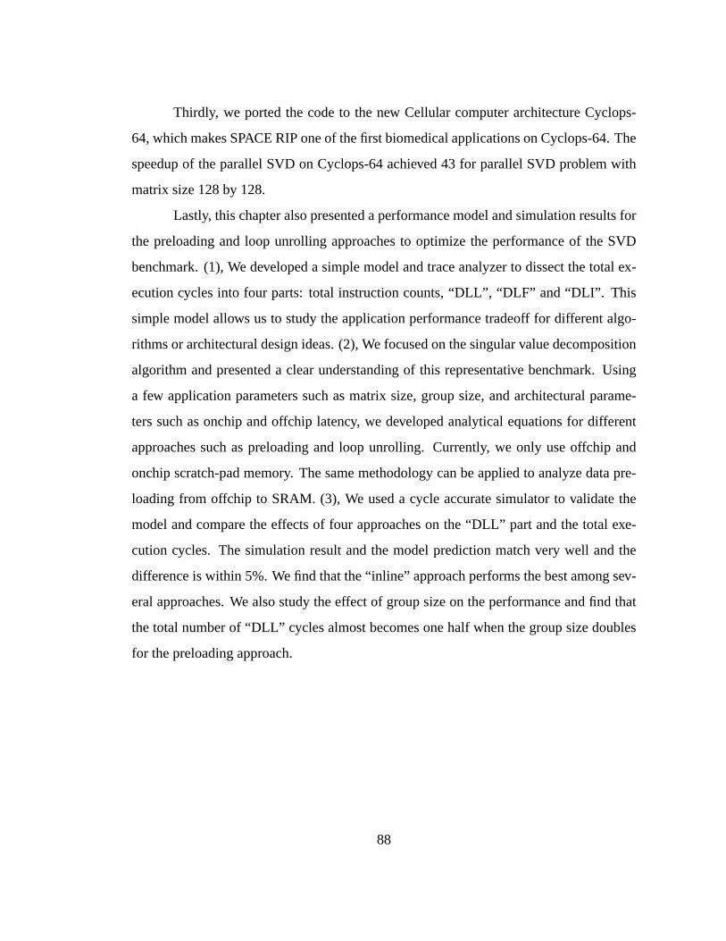
Thirdly, we ported the code to the new Cellular computer architecture Cyclops-

64, which makes SPACE RIP one of the first biomedical applications on Cyclops-64. The

speedup of the parallel SVD on Cyclops-64 achieved 43 for parallel SVD problem with

matrix size 128 by 128.

Lastly, this chapter also presented a performance model andsimulation results for

the preloading and loop unrolling approaches to optimize the performance of the SVD

benchmark. (1), We developed a simple model and trace analyzer to dissect the total ex-

ecution cycles into four parts: total instruction counts, “DLL”, “DLF” and “DLI”. This

simple model allows us to study the application performancetradeoff for different algo-

rithms or architectural design ideas. (2), We focused on thesingular value decomposition

algorithm and presented a clear understanding of this representative benchmark. Using

a few application parameters such as matrix size, group size, and architectural parame-

ters such as onchip and offchip latency, we developed analytical equations for different

approaches such as preloading and loop unrolling. Currently, we only use offchip and

onchip scratch-pad memory. The same methodology can be applied to analyze data pre-

loading from offchip to SRAM. (3), We used a cycle accurate simulator to validate the

model and compare the effects of four approaches on the “DLL”part and the total exe-

cution cycles. The simulation result and the model prediction match very well and the

difference is within 5%. We find that the “inline” approach performs the best among sev-

eral approaches. We also study the effect of group size on theperformance and find that

the total number of “DLL” cycles almost becomes one half whenthe group size doubles

for the preloading approach.

88

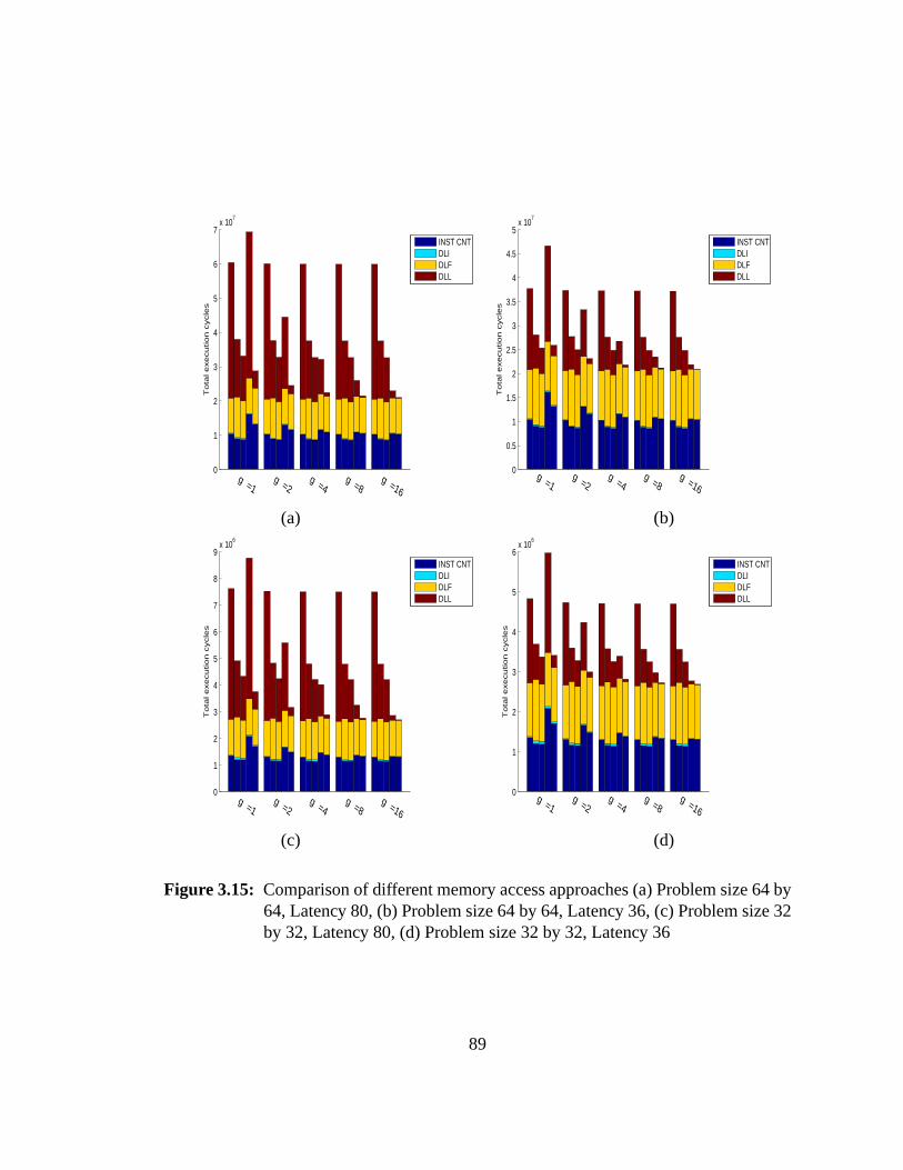
0

1

2

3

4

5

6

7x 10

7

To

tal e

xe

cu

tio

n c

ycle

s

g =1

g =2

g =4

g =8

g =16

INST CNTDLIDLFDLL

0

0.5

1

1.5

2

2.5

3

3.5

4

4.5

5x 10

7

To

tal e

xe

cu

tio

n c

ycle

s

g =1

g =2

g =4

g =8

g =16

INST CNTDLIDLFDLL

(a) (b)

0

1

2

3

4

5

6

7

8

9x 10

6

To

tal e

xe

cu

tio

n c

ycle

s

g =1

g =2

g =4

g =8

g =16

INST CNTDLIDLFDLL

0

1

2

3

4

5

6x 10

6

To

tal e

xe

cu

tio

n c

ycle

s

g =1

g =2

g =4

g =8

g =16

INST CNTDLIDLFDLL

(c) (d)

Figure 3.15: Comparison of different memory access approaches (a) Problem size 64 by64, Latency 80, (b) Problem size 64 by 64, Latency 36, (c) Problem size 32by 32, Latency 80, (d) Problem size 32 by 32, Latency 36

89

1 2 4 8 16 320

1

2

3

4

5

6

7

8x 10

7

Num of threads

Instr

ucti

on

Cycle

s

Performance of Different Approaches on Multiple Threads, problem size 64 by 64, offchip latency 80

BaseMemcpyUnroll8unroll4Inline

Figure 3.16: Performance of different approaches on multiple threads

90

Chapter 4

GENERATION OF TACTILE GRAPHICS WITH MULTILEVEL

DIGITAL HALFTONING

4.1 Introduction

Humans receive all of their information about the world using one or more of the

five senses [95]: the gustatory sense, the olfactory sense, the auditory sense, the tactual

sense, and the visual sense. The visual sense has the highestbandwidth among the five

senses, making the illustration of ideas and concepts visually through images and graphics

an efficient means of communications. Loss of one of the five senses requires information

to be translated from one sense to another. One possible translation is the visual to audio

translation, e.g., screen reading software [96] interactswith speech synthesizers to enable

visually impaired individuals to access information through voice output. Screen readers,

however, can only read text, thus limiting access to graphicinformation.

Another possible information translation is the visual to tactile translation. The

visual to tactile translation can further help with understanding graphics, including ob-

ject shape and texture, while the visual to audio translation is suitable for understanding

concepts. Many techniques have been proposed to translate text and graphics information

into the tactile modality. In 1934, Louis Braille invented the Braille system for sightless

reading and writing, regarded as one of the most significant contributions to the education

of blind individuals [97]. This approach, however, is also limited to text-based informa-

tion. Tactile pattern and graphics access were also made possible with the invention of

the Optacon [98], which can convert a visual image into a pattern of pin vibrations that

91

can be read with one finger. Martinet al. [99] developed methods to present business

graphics to blind individuals, converting pie charts, bar charts and other representations

into the tactile modality.

Recent work includes [100, 101], which successfully developed software algo-

rithms for the automatic generation of tactile graphics. Meaningful information, includ-

ing edges and boundaries, is identified and extracted from visual image data via a multi-

step procedure. A shortcoming of simple line edge-map-based tactile graphics is that

the resulting edges often intersect and do not form closed structures. This shortcoming

can be addressed by segmentation procedures as well as multi-resolution edge detection

[102–104]. Closed contours often yield improved representations over simple line edge-

map-based representations.

A shortcoming of binary edge maps, whether generated from anedge detection

algorithm or segmentation procedures, is that features andregions are identified only by

their boundaries. Such identification yields no information on the grayscale value, color,

or texture of a given region. To address the issue of tactile texture representation, a tac-

tile texture generation method for the TIE (Tactile Image Enhancer) [105] was proposed

[106]. In this work, the human tactile system and tactile printing process model, along

with binary halftoning algorithms, are developed and optimized for the TIE printer.

Digital halftoning is a method for rendering the illusion ofcontinuous-tone pic-

tures on display or printing devices that are capable of producing only a limited range of

tone levels. Recent research has yielded numerous halftoning methods, many of which

are reviewed in [107–109]. Halftoning algorithms generatebinary on/off pixel patterns

to create the visual illusion of gray level or color. This is possible due to the low pass

nature of the human visual system, which averages black dotsand white space to yield

the perceived grayscale level. A similar approach can be taken to produce tactile textures,

utilizing the low pass property of the human tactile system [106].

Although the generation of tactile patterns through halftoning procedures appears

92

promising, numerous open problems must be addressed beforethe method can be used

in practice. For instance, halftoning algorithms must be applied and optimized to other

tactile printers, such as the TIGER embossing tactile printer [105], which is a commonly

used tactile printer that has the ability to punch dots of different heights on the paper, and

thus can be regarded as a multilevel system. Also, differenthalftoning algorithms need to

be implemented to generate and compare different texture patterns, such as the determin-

istic textures or stochastic textures, clustered dot textures or dispersed dot textures, etc.

This research addresses these specific issues.

To address the first issue, multilevel halftoning algorithms are implemented on

the TIGER printer to generate tactile texture patterns. As an extension of binary halfton-

ing, multilevel halftoning techniques are commonly adopted on printers that can generate

several output levels. Therefore, multilevel halftoning is a natural choice for the TIGER

printer to take advantage of the printer’s variable-heightpunching ability. To address the

second issue, four different multilevel halftoning algorithms, including AM, Bayer’s, er-

ror diffusion, and green noise halftoning [108–112], are implemented, of which, AM

and Bayer’s are deterministic algorithms and the latter two are stochastic algorithms.

Experiments are conducted to compare the halftoning-basedapproach with the simple

commonly utilized thresholding-based approach. It is shown that the halftoning-based

approaches achieved significant improvement in terms of texture pattern discrimination

ability and that green noise halftoning achieved the best performance result amongst the

four types of halftoning algorithms.

The remainder of this chapter is organized as follows. A brief review of tactile

printing and the TIGER printer hardware and software are presented in section 4.2. In sec-

tions 4.3 and 4.4 we discuss the basics of halftoning techniques and multilevel halftoning

algorithms specifically adapted for the TIGER printer. Section 4.5 presents the experi-

ment design, protocol, and evaluation results. Finally, a brief summary is presented in

section 4.7.

93

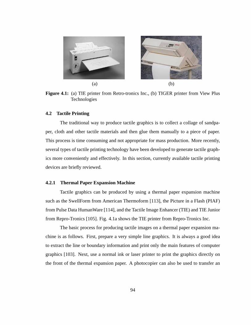
(a) (b)

Figure 4.1: (a) TIE printer from Retro-tronics Inc., (b) TIGER printer from View PlusTechnologies

4.2 Tactile Printing

The traditional way to produce tactile graphics is to collect a collage of sandpa-

per, cloth and other tactile materials and then glue them manually to a piece of paper.

This process is time consuming and not appropriate for mass production. More recently,

several types of tactile printing technology have been developed to generate tactile graph-

ics more conveniently and effectively. In this section, currently available tactile printing

devices are briefly reviewed.

4.2.1 Thermal Paper Expansion Machine

Tactile graphics can be produced by using a thermal paper expansion machine

such as the SwellForm from American Thermoform [113], the Picture in a Flash (PIAF)

from Pulse Data HumanWare [114], and the Tactile Image Enhancer (TIE) and TIE Junior

from Repro-Tronics [105]. Fig. 4.1a shows the TIE printer from Repro-Tronics Inc.

The basic process for producing tactile images on a thermal paper expansion ma-

chine is as follows. First, prepare a very simple line graphics. It is always a good idea

to extract the line or boundary information and print only the main features of computer

graphics [103]. Next, use a normal ink or laser printer to print the graphics directly on

the front of the thermal expansion paper. A photocopier can also be used to transfer an

94

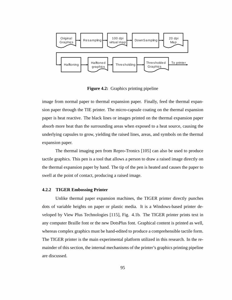
Origina lGraphics

20 dpiMap

Resampling100 dpi

virtua l mapDownSampling

Halftonedgraphics

ThresholdedGraphics

Halftoning ThresholdingTo printer

Figure 4.2: Graphics printing pipeline

image from normal paper to thermal expansion paper. Finally, feed the thermal expan-

sion paper through the TIE printer. The micro-capsule coating on the thermal expansion

paper is heat reactive. The black lines or images printed on the thermal expansion paper

absorb more heat than the surrounding areas when exposed to aheat source, causing the

underlying capsules to grow, yielding the raised lines, areas, and symbols on the thermal

expansion paper.

The thermal imaging pen from Repro-Tronics [105] can also be used to produce

tactile graphics. This pen is a tool that allows a person to draw a raised image directly on

the thermal expansion paper by hand. The tip of the pen is heated and causes the paper to

swell at the point of contact, producing a raised image.

4.2.2 TIGER Embossing Printer

Unlike thermal paper expansion machines, the TIGER printerdirectly punches

dots of variable heights on paper or plastic media. It is a Windows-based printer de-

veloped by View Plus Technologies [115], Fig. 4.1b. The TIGER printer prints text in

any computer Braille font or the new DotsPlus font. Graphicalcontent is printed as well,

whereas complex graphics must be hand-edited to produce a comprehensible tactile form.

The TIGER printer is the main experimental platform utilized in this research. In the re-

mainder of this section, the internal mechanisms of the printer’s graphics printing pipeline

are discussed.

95

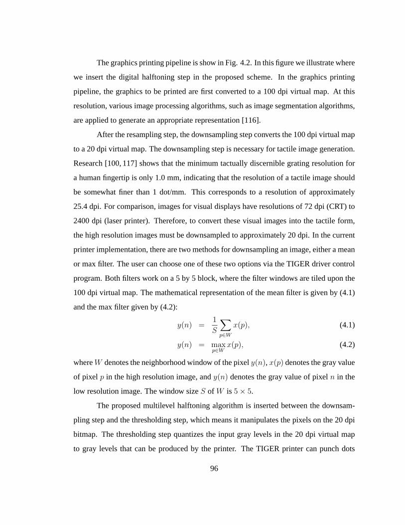
The graphics printing pipeline is show in Fig. 4.2. In this figure we illustrate where

we insert the digital halftoning step in the proposed scheme. In the graphics printing

pipeline, the graphics to be printed are first converted to a 100 dpi virtual map. At this

resolution, various image processing algorithms, such as image segmentation algorithms,

are applied to generate an appropriate representation [116].

After the resampling step, the downsampling step converts the 100 dpi virtual map

to a 20 dpi virtual map. The downsampling step is necessary for tactile image generation.

Research [100, 117] shows that the minimum tactually discernible grating resolution for

a human fingertip is only 1.0 mm, indicating that the resolution of a tactile image should

be somewhat finer than 1 dot/mm. This corresponds to a resolution of approximately

25.4 dpi. For comparison, images for visual displays have resolutions of 72 dpi (CRT) to

2400 dpi (laser printer). Therefore, to convert these visual images into the tactile form,

the high resolution images must be downsampled to approximately 20 dpi. In the current

printer implementation, there are two methods for downsampling an image, either a mean

or max filter. The user can choose one of these two options via the TIGER driver control

program. Both filters work on a 5 by 5 block, where the filter windows are tiled upon the

100 dpi virtual map. The mathematical representation of themean filter is given by (4.1)

and the max filter given by (4.2):

y(n) =1

S

∑

p∈W

x(p), (4.1)

y(n) = maxp∈W

x(p), (4.2)

whereW denotes the neighborhood window of the pixely(n), x(p) denotes the gray value

of pixel p in the high resolution image, andy(n) denotes the gray value of pixeln in the

low resolution image. The window sizeS of W is 5 × 5.

The proposed multilevel halftoning algorithm is inserted between the downsam-

pling step and the thresholding step, which means it manipulates the pixels on the 20 dpi

bitmap. The thresholding step quantizes the input gray levels in the 20 dpi virtual map

to gray levels that can be produced by the printer. The TIGER printer can punch dots

96

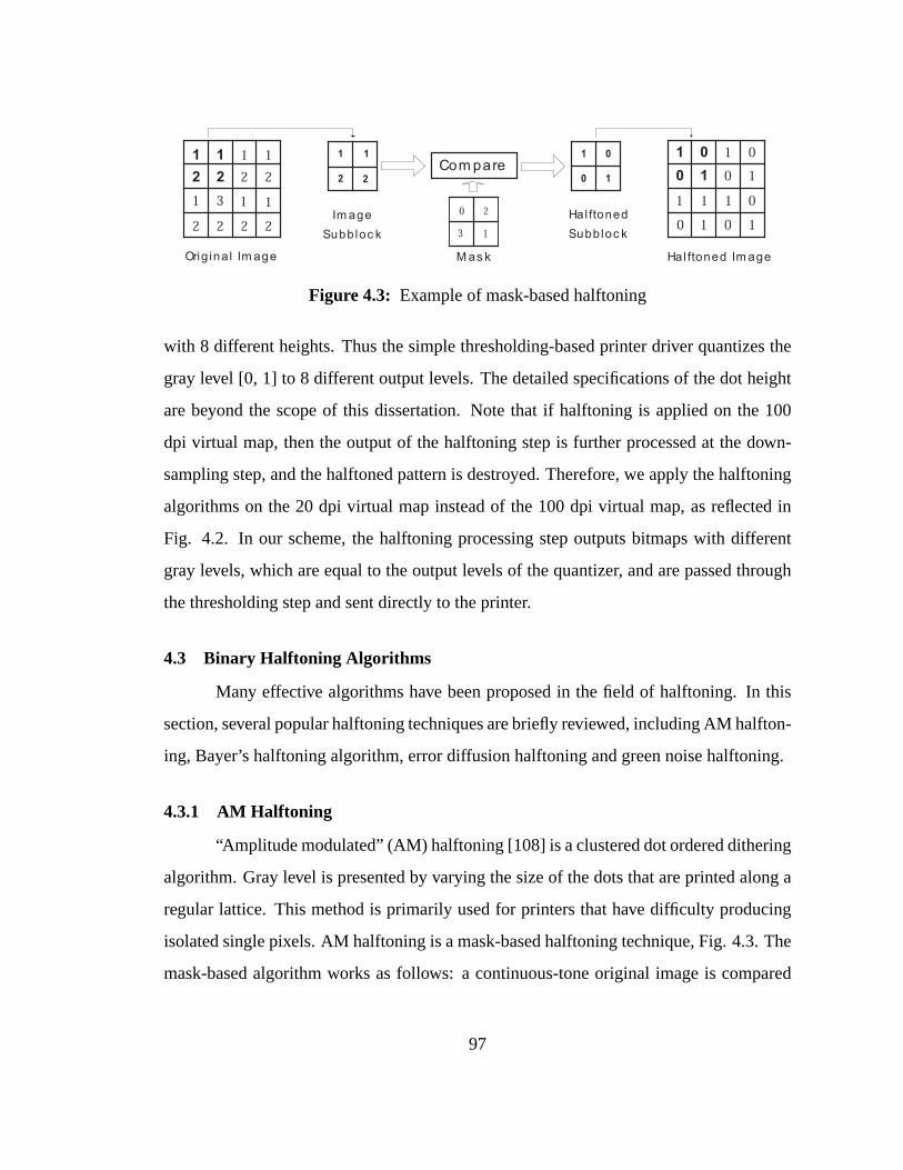
0

13

2

1

2 2

1 3

2 2 2

1

2

1 1 1

2 2

0 0

1 1

1 1

1 1

0 0

1 1

0

1

22

1

Com pare1

10

0

1 0

0

Orig ina l Im age Hal ftoned Im age

Im age

Subbloc k

Hal ftoned

Subbloc k

M as k

1

Figure 4.3: Example of mask-based halftoning

with 8 different heights. Thus the simple thresholding-based printer driver quantizes the

gray level [0, 1] to 8 different output levels. The detailed specifications of the dot height

are beyond the scope of this dissertation. Note that if halftoning is applied on the 100

dpi virtual map, then the output of the halftoning step is further processed at the down-

sampling step, and the halftoned pattern is destroyed. Therefore, we apply the halftoning

algorithms on the 20 dpi virtual map instead of the 100 dpi virtual map, as reflected in

Fig. 4.2. In our scheme, the halftoning processing step outputs bitmaps with different

gray levels, which are equal to the output levels of the quantizer, and are passed through

the thresholding step and sent directly to the printer.

4.3 Binary Halftoning Algorithms

Many effective algorithms have been proposed in the field of halftoning. In this

section, several popular halftoning techniques are brieflyreviewed, including AM halfton-

ing, Bayer’s halftoning algorithm, error diffusion halftoning and green noise halftoning.

4.3.1 AM Halftoning

“Amplitude modulated” (AM) halftoning [108] is a clustereddot ordered dithering

algorithm. Gray level is presented by varying the size of thedots that are printed along a

regular lattice. This method is primarily used for printersthat have difficulty producing

isolated single pixels. AM halftoning is a mask-based halftoning technique, Fig. 4.3. The

mask-based algorithm works as follows: a continuous-tone original image is compared

97

to the mask, where each pixel of the original image is converted directly into a binary

dot based on a pixel-by-pixel comparison with the mask. Pixels with a gray level greater

than their corresponding threshold in the mask are converted to “on” pixels in the final

halftoned image, while pixels less than the corresponding thresholds are turned “off”. The

mask is tiled end-to-end on the original image. The mask is generated such that the output

“on” pixels tend to cluster together. One example of the AM mask [109] is shown in Fig.

4.4a. The AM halftoned pattern of a gray level ramp is shown inFig. 4.5b.

4.3.2 Bayer’s Halftoning Algorithm

Bayer’s algorithm [110] is a dispersed dot ordered ditheringtechnique. This tech-

nique is also a mask-based method, but it turns pixels “on” individually without grouping

them into clusters. In Bayer’s mask, consecutive thresholdsare dispersed as much as

possible, an example [108] of which is shown in Fig. 4.4b. By maintaining the size of

printed dots for all gray levels as an individual pixel, dispersed dot halftoning techniques

vary the spacing between printed dots according to the gray level, earning the name “fre-

quency modulated” or FM halftoning. The Bayer’s method produces periodic structures.

In the visual case, these structures introduce an unnaturalvisual appearance. However,

the periodic structure may be helpful for perception in the tactile case, which is why we

include Bayer’s algorithm here and implement it into the TIGER printer driver. Like AM

halftoning, the Bayer halftoning algorithm is a deterministic halftoning algorithm. The

Bayer’s halftoned pattern of a gray level ramp is shown in Fig.4.5c.

4.3.3 Error Diffusion Halftoning

The error diffusion halftoning technique was proposed by Floyd and Steinberg

[111]. This algorithm is a stochastic dispersed dot halftoning. Error diffusion also keeps

the dot size fixed as a single pixel, and the required illusionof continuous tone is achieved

by varying the distance between printed dots. This process adopts a stochastic method

for quantizing the gray level of each pixel. The quantization error produced in each of

98

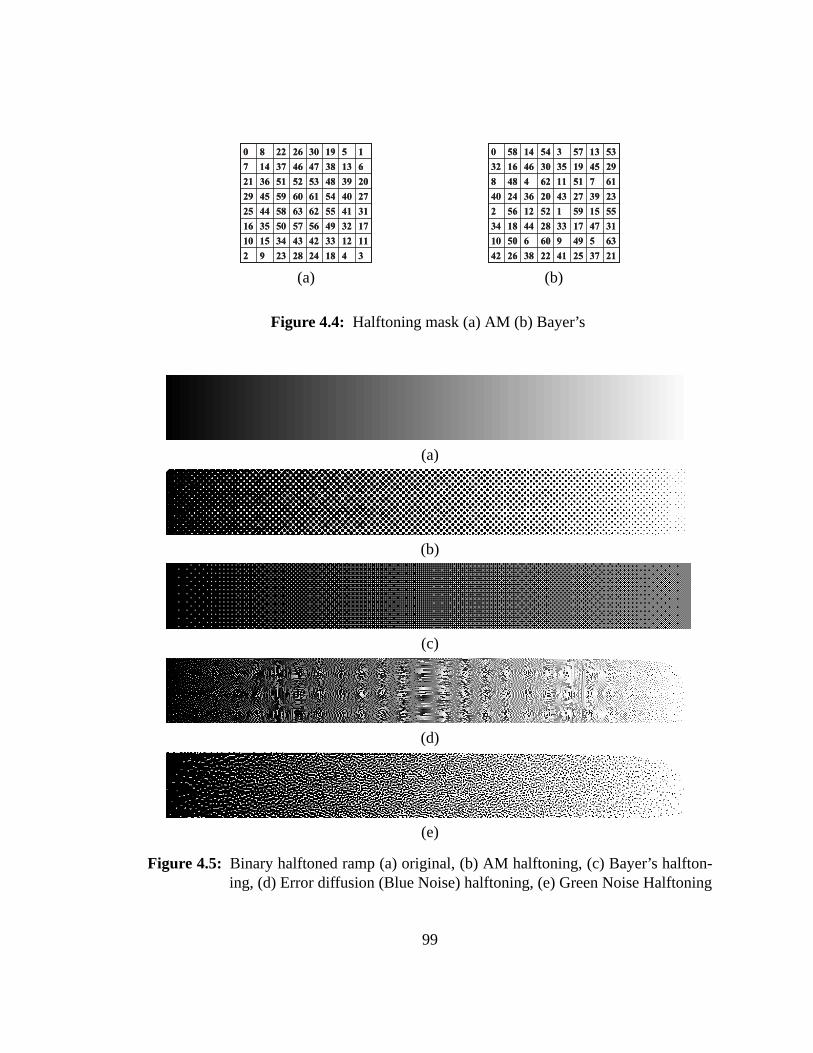
341824282392

1112334243341510

1732495657503516

3141556263584425

2740546160594529

2039485352513621

61338474637147

151930262280

341824282392

1112334243341510

1732495657503516

3141556263584425

2740546160594529

2039485352513621

61338474637147

151930262280

2137254122382642

6354996065010

3147173328441834

55155915212562

2339274320362440

6175111624488

2945193530461632

53135735414580

2137254122382642

6354996065010

3147173328441834

55155915212562

2339274320362440

6175111624488

2945193530461632

53135735414580

(a) (b)

Figure 4.4: Halftoning mask (a) AM (b) Bayer’s

(a)

(b)

(c)

(d)

(e)

Figure 4.5: Binary halftoned ramp (a) original, (b) AM halftoning, (c) Bayer’s halfton-ing, (d) Error diffusion (Blue Noise) halftoning, (e) Green Noise Halftoning

99

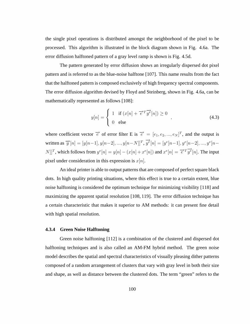
the single pixel operations is distributed amongst the neighborhood of the pixel to be

processed. This algorithm is illustrated in the block diagram shown in Fig. 4.6a. The

error diffusion halftoned pattern of a gray level ramp is shown is Fig. 4.5d.

The pattern generated by error diffusion shows an irregularly dispersed dot pixel

pattern and is referred to as the blue-noise halftone [107].This name results from the fact

that the halftoned pattern is composed exclusively of high frequency spectral components.

The error diffusion algorithm devised by Floyd and Steinberg, shown in Fig. 4.6a, can be

mathematically represented as follows [108]:

y[n] =

1 if (x[n] + −→e T−→ye [n]) ≥ 0

0 else, (4.3)

where coefficient vector−→e of error filter E is−→e = [e1, e2, ..., eN ]T , and the output is

written as−→y [n] = [y[n−1], y[n−2], ..., y[n−N ]]T ,−→ye [n] = [ye[n−1], ye[n−2], ..., ye[n−

N ]]T , which follows fromye[n] = y[n]− (x[n] +xe[n]) andxe[n] = −→e T−→ye [n]. The input

pixel under consideration in this expression isx[n].

An ideal printer is able to output patterns that are composedof perfect square black

dots. In high quality printing situations, where this effect is true to a certain extent, blue

noise halftoning is considered the optimum technique for minimizing visibility [118] and

maximizing the apparent spatial resolution [108, 119]. Theerror diffusion technique has

a certain characteristic that makes it superior to AM methods: it can present fine detail

with high spatial resolution.

4.3.4 Green Noise Halftoning

Green noise halftoning [112] is a combination of the clustered and dispersed dot

halftoning techniques and is also called an AM-FM hybrid method. The green noise

model describes the spatial and spectral characteristics of visually pleasing dither patterns

composed of a random arrangement of clusters that vary with gray level in both their size

and shape, as well as distance between the clustered dots. The term “green” refers to the

100

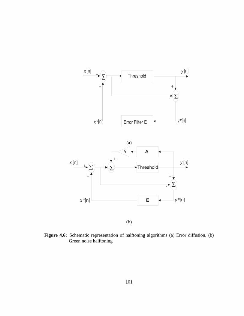
Σ

Σ

x [n] y [n]

y e[n]x e[n]

+

+

+

-

Error Filter E

Threshold

(a)

E

Σ

Σx [n] y [n]

y e[n]x e[n]

+

+

+

-

Σ

Ah

+

+ Threshold

(b)

Figure 4.6: Schematic representation of halftoning algorithms (a) Error diffusion, (b)Green noise halftoning

101

mid-frequency content of the corresponding halftone patterns, as green light is the mid-

frequency of white light. The green noise halftoned patternof a gray level ramp is shown

in Fig. 4.5e.

In green noise halfoned images, the minority pixel clustersare distributed ho-

mogenously. The green noise halftone is generated as an extension to the error diffusion

technique proposed by Levien [112] and referred to as the error diffusion with output

dependent feedback. The block diagram of the algorithm is shown in Fig. 4.6b. In this

algorithm, a weighted sum of previous output pixels is used to vary the threshold. This

makes minority pixels more likely to occur in clusters. The amount of clustering is con-

trolled through the hysteresis constanth. Large values ofh cause large clustering and

small values lead to smaller clusters.

Levien’s algorithm is precisely defined as follows [108]:

y[n] =

1 if (x[n] + −→e T−→ye [n] + h−→a T−→y [n]) ≥ 0

0 else, (4.4)

where−→a = [a1, a2, ..., aN ]T ,−→e = [e1, e2, ..., eN ]T ,∑N

i=0 ai = 1,∑N

i=0 ei = 1, and the

output−→y [n] and−→ye [n] are defined as before. The coefficient vector−→e of error filter E,

coefficient vector−→a of hysteresis filter A, and hysteresis constanth can take on a wide

range of values, including special cases such as Floyd-Steinberg [111], Jarvis [120] and

Stucki [121] filter coefficients.

4.4 Multilevel Halftoning Algorithms

In ink and laser printing, technologies that can generate more than two output

levels are becoming increasingly common [109]. The image quality studies by Huang

et al. [122] demonstrated that a few intermediate output levels can provide a substantial

improvement to halftoned images. Therefore, multilevel halftoning [123, 124] extensions

from traditional binary halftoning algorithms are also becoming more common. In this

102

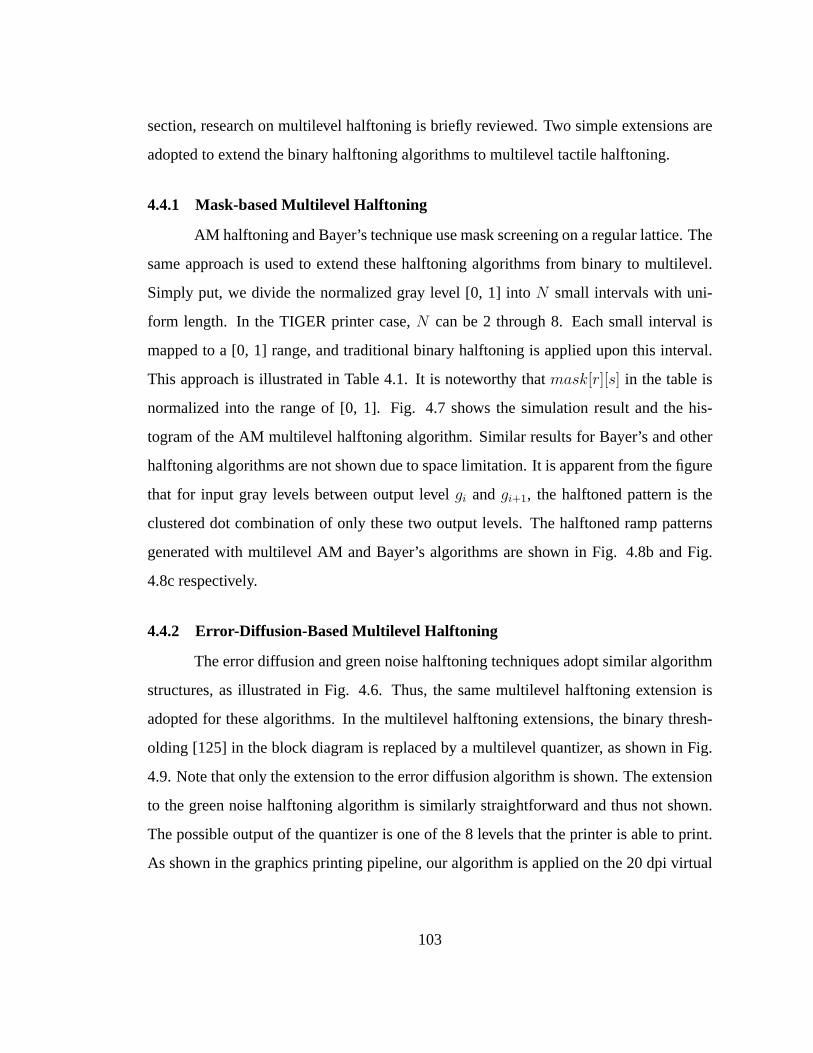
section, research on multilevel halftoning is briefly reviewed. Two simple extensions are

adopted to extend the binary halftoning algorithms to multilevel tactile halftoning.

4.4.1 Mask-based Multilevel Halftoning

AM halftoning and Bayer’s technique use mask screening on a regular lattice. The

same approach is used to extend these halftoning algorithmsfrom binary to multilevel.

Simply put, we divide the normalized gray level [0, 1] intoN small intervals with uni-

form length. In the TIGER printer case,N can be 2 through 8. Each small interval is

mapped to a [0, 1] range, and traditional binary halftoning is applied upon this interval.

This approach is illustrated in Table 4.1. It is noteworthy thatmask[r][s] in the table is

normalized into the range of [0, 1]. Fig. 4.7 shows the simulation result and the his-

togram of the AM multilevel halftoning algorithm. Similar results for Bayer’s and other

halftoning algorithms are not shown due to space limitation. It is apparent from the figure

that for input gray levels between output levelgi andgi+1, the halftoned pattern is the

clustered dot combination of only these two output levels. The halftoned ramp patterns

generated with multilevel AM and Bayer’s algorithms are shown in Fig. 4.8b and Fig.

4.8c respectively.

4.4.2 Error-Diffusion-Based Multilevel Halftoning

The error diffusion and green noise halftoning techniques adopt similar algorithm

structures, as illustrated in Fig. 4.6. Thus, the same multilevel halftoning extension is

adopted for these algorithms. In the multilevel halftoningextensions, the binary thresh-

olding [125] in the block diagram is replaced by a multilevelquantizer, as shown in Fig.

4.9. Note that only the extension to the error diffusion algorithm is shown. The extension

to the green noise halftoning algorithm is similarly straightforward and thus not shown.

The possible output of the quantizer is one of the 8 levels that the printer is able to print.

As shown in the graphics printing pipeline, our algorithm isapplied on the 20 dpi virtual

103

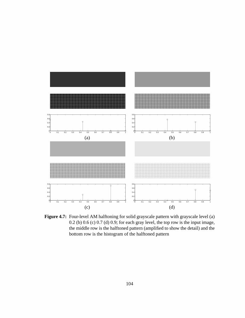
0 0.1 0.2 0.3 0.4 0.5 0.6 0.7 0.8 0.9 10

0.2

0.4

0.6

0.8

0 0.1 0.2 0.3 0.4 0.5 0.6 0.7 0.8 0.9 10

0.2

0.4

0.6

0.8

(a) (b)

0 0.1 0.2 0.3 0.4 0.5 0.6 0.7 0.8 0.9 10

0.2

0.4

0.6

0.8

0 0.1 0.2 0.3 0.4 0.5 0.6 0.7 0.8 0.9 10

0.2

0.4

0.6

0.8

(c) (d)

Figure 4.7: Four-level AM halftoning for solid grayscale pattern with grayscale level (a)0.2 (b) 0.6 (c) 0.7 (d) 0.9; for each gray level, the top row is the input image,the middle row is the halftoned pattern (amplified to show thedetail) and thebottom row is the histogram of the halftoned pattern

104

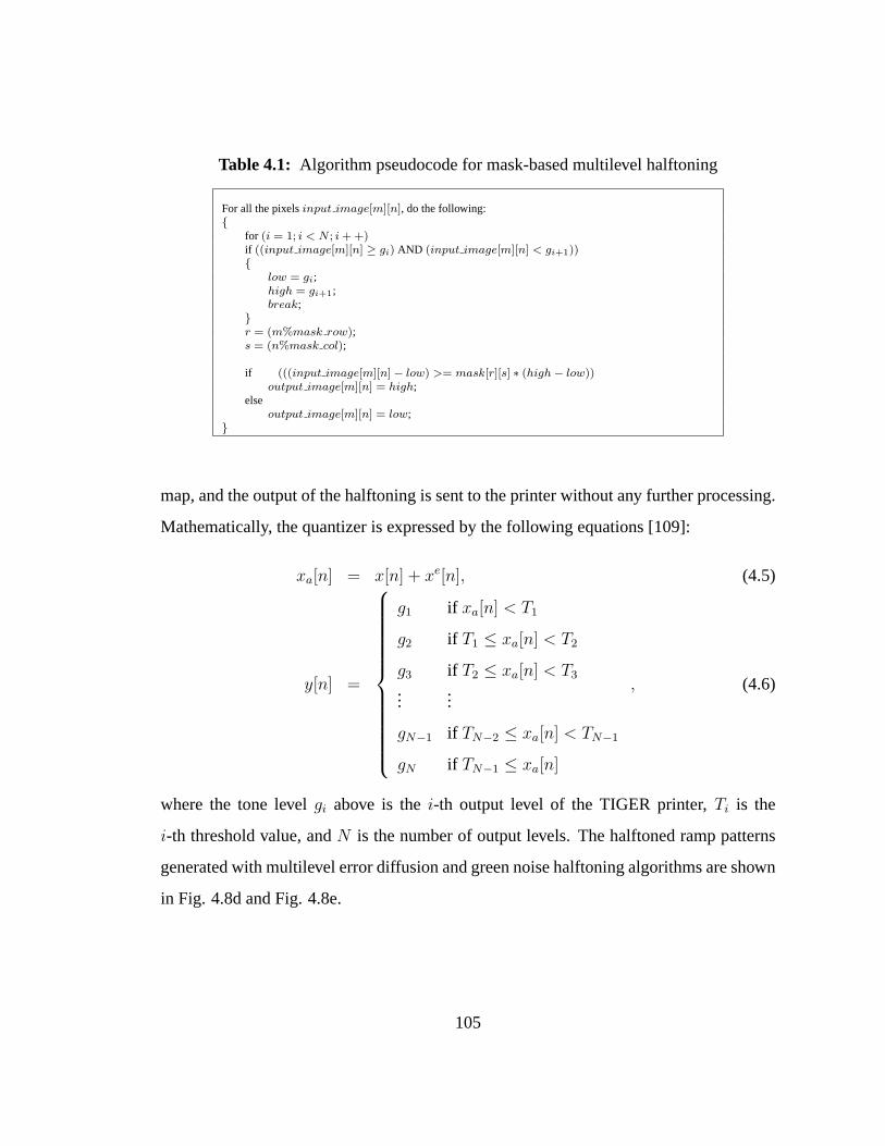
Table 4.1: Algorithm pseudocode for mask-based multilevel halftoning

For all the pixelsinput image[m][n], do the following:{

for (i = 1; i < N ; i + +)if ((input image[m][n] ≥ gi) AND (input image[m][n] < gi+1)){

low = gi;high = gi+1;break;

}r = (m%mask row);s = (n%mask col);

if (((input image[m][n] − low) >= mask[r][s] ∗ (high − low))output image[m][n] = high;

elseoutput image[m][n] = low;

}

map, and the output of the halftoning is sent to the printer without any further processing.

Mathematically, the quantizer is expressed by the following equations [109]:

xa[n] = x[n] + xe[n], (4.5)

y[n] =

g1 if xa[n] < T1

g2 if T1 ≤ xa[n] < T2

g3 if T2 ≤ xa[n] < T3

......

gN−1 if TN−2 ≤ xa[n] < TN−1

gN if TN−1 ≤ xa[n]

, (4.6)

where the tone levelgi above is thei-th output level of the TIGER printer,Ti is the

i-th threshold value, andN is the number of output levels. The halftoned ramp patterns

generated with multilevel error diffusion and green noise halftoning algorithms are shown

in Fig. 4.8d and Fig. 4.8e.

105

(a)

(b)

(c)

(d)

(e)

Figure 4.8: Multilevel halftoned Ramp with four output levels (a) original , (b) AMhalftoning , (c) Bayer’s Halftoning, (d) error diffusion (bue noise) halftoning,(e) green Noise Halftoning

106

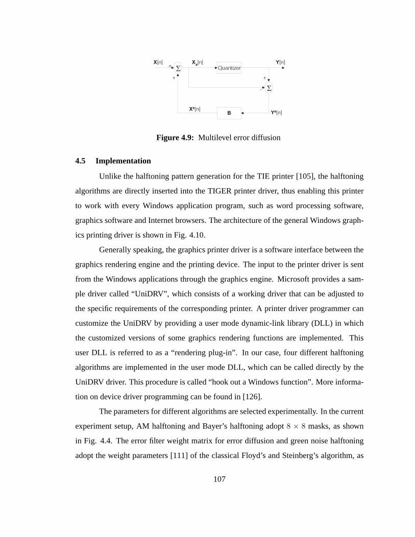
Quantizer

B

Σ

Σ

X[n] Y[n]

Ye[n]Xe[n]

+

+

+

-

Xa[n]

Figure 4.9: Multilevel error diffusion

4.5 Implementation

Unlike the halftoning pattern generation for the TIE printer [105], the halftoning

algorithms are directly inserted into the TIGER printer driver, thus enabling this printer

to work with every Windows application program, such as wordprocessing software,

graphics software and Internet browsers. The architectureof the general Windows graph-

ics printing driver is shown in Fig. 4.10.

Generally speaking, the graphics printer driver is a software interface between the

graphics rendering engine and the printing device. The input to the printer driver is sent

from the Windows applications through the graphics engine.Microsoft provides a sam-

ple driver called “UniDRV”, which consists of a working driver that can be adjusted to

the specific requirements of the corresponding printer. A printer driver programmer can

customize the UniDRV by providing a user mode dynamic-link library (DLL) in which

the customized versions of some graphics rendering functions are implemented. This

user DLL is referred to as a “rendering plug-in”. In our case,four different halftoning

algorithms are implemented in the user mode DLL, which can becalled directly by the

UniDRV driver. This procedure is called “hook out a Windows function”. More informa-

tion on device driver programming can be found in [126].

The parameters for different algorithms are selected experimentally. In the current

experiment setup, AM halftoning and Bayer’s halftoning adopt 8 × 8 masks, as shown

in Fig. 4.4. The error filter weight matrix for error diffusion and green noise halftoning

adopt the weight parameters [111] of the classical Floyd’s and Steinberg’s algorithm, as

107

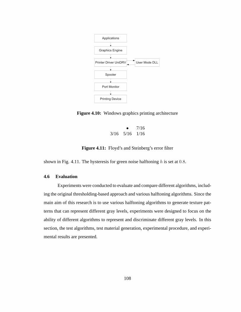
Applications

Graphics Engine

Printer Driver UniDRV

Spooler

Port Monitor

Printing Device

User Mode DLL

Figure 4.10: Windows graphics printing architecture

• 7/163/16 5/16 1/16

Figure 4.11: Floyd’s and Steinberg’s error filter

shown in Fig. 4.11. The hysteresis for green noise halftoning h is set at0.8.

4.6 Evaluation

Experiments were conducted to evaluate and compare different algorithms, includ-

ing the original thresholding-based approach and various halftoning algorithms. Since the

main aim of this research is to use various halftoning algorithms to generate texture pat-

terns that can represent different gray levels, experiments were designed to focus on the

ability of different algorithms to represent and discriminate different gray levels. In this

section, the test algorithms, test material generation, experimental procedure, and experi-

mental results are presented.

108

4.6.1 Test Algorithms

There are four types of halftoning algorithms to be evaluated: AM, Bayer’s, Error

diffusion and Green noise halftoning algorithms. For each algorithm, we can use binary

halftoning, in which the output pattern is composed of either “no dot” (blank paper) or

highest dot. Alternatively, we can use three-level halftoning, in which the output pattern

is composed of three possibilities: “no dot”, dot with medium height, or highest dot.

Similarly, four-level or five-level halftoning algorithmscan also be implemented.

Of interest is the determination of whether or not the multilevel halftoning al-

gorithms generate better tactile patterns in the sense of better discrimination ability and

effectiveness. Also of interest is the optimal number of output levels, i.e., which of the

binary, three-level or four-level halftoning, etc is the best choice. Our hypothesis is that

more output levels do not necessarily result in better discrimination ability. If we use too

many output levels, then the height difference between two neighboring output levels be-

comes negligible. Since the multilevel halftoning algorithms are designed such that a gray

level is represented by the combination of two neighboring output levels, the texture may

not be apparent enough to be discriminated with the sense of touch if the two neighboring

output heights are insufficiently distinct.

Therefore, different algorithms with different output levels are included in the

experiments in order to answer the previous questions and totest whether our hypothesis

is correct. Preliminary tests show that tactile patterns generated with five output levels

are insufficiently distinct to be discriminated. Therefore, five-level algorithms are not

included in the presented result. The algorithms tested arelisted in the first column of

Table 4.3.

4.6.2 Test Material

The experiments conducted are discrimination experimentsin which subjects ex-

plore freely left and right tactile image pairs and tell whether they are different or not.

Therefore, the test materials include image pairs. Each image is a square of one specific

109

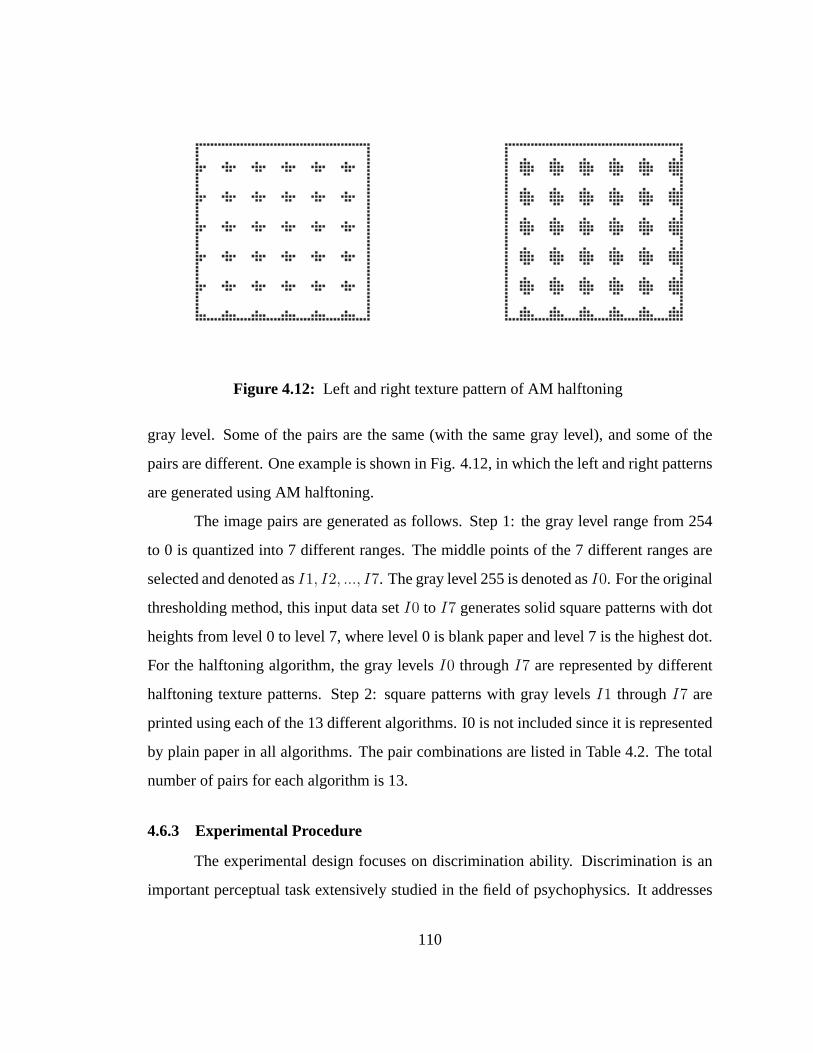
Figure 4.12: Left and right texture pattern of AM halftoning

gray level. Some of the pairs are the same (with the same gray level), and some of the

pairs are different. One example is shown in Fig. 4.12, in which the left and right patterns

are generated using AM halftoning.

The image pairs are generated as follows. Step 1: the gray level range from 254

to 0 is quantized into 7 different ranges. The middle points of the 7 different ranges are

selected and denoted asI1, I2, ..., I7. The gray level 255 is denoted asI0. For the original

thresholding method, this input data setI0 to I7 generates solid square patterns with dot

heights from level 0 to level 7, where level 0 is blank paper and level 7 is the highest dot.

For the halftoning algorithm, the gray levelsI0 throughI7 are represented by different

halftoning texture patterns. Step 2: square patterns with gray levelsI1 throughI7 are

printed using each of the 13 different algorithms. I0 is not included since it is represented

by plain paper in all algorithms. The pair combinations are listed in Table 4.2. The total

number of pairs for each algorithm is 13.

4.6.3 Experimental Procedure

The experimental design focuses on discrimination ability. Discrimination is an

important perceptual task extensively studied in the field of psychophysics. It addresses

110

Table 4.2: Test pairs

Type of Pair Combinations

Left and right Different (I1, I2), (I2, I3), (I3, I4), (I4, I5), (I5, I6), (I6, I7)Left and right Same (I1, I1), (I2, I2), (I3, I3), (I4, I4), (I5, I5), (I6, I6), (I7, I7)

the question “Is one stimulus different from another one?”.In our experiments, the test

subjects explore two tactile objects, only by the sense of touch, and indicate whether they

think they are the same or not.

Ten sighted test subjects participated voluntarily in the experiment. Seven subjects

are male and three subjects are female. It is widely believedthat touch sensitivity varies

little from subject to subject, and that there is no statistical difference between the sighted

and unsighted populations [127, 128]. Therefore, information on how individuals with

visual impairment perceive can be inferred from the sightedsubject results.

Each subject was asked to perform a discrimination task using one complete set of

13 pairs per algorithm× 13 algorithms. Subjects were seated at a table, blindfoldedand

presented with a set of13 × 13 sheets in random order. Subjects were briefly introduced

to the basic features of different algorithms at the beginning of the experiments. For each

sheet, subjects freely explored the pairs of tactile imageson the sheet for a time period.

This gives the subjects enough time to glean information about the texture/gray level of

the images. Then the subjects were asked to report whether the images felt the same or

different. Subjects also could make a guess if they could notsay one way or the other.

During this procedure, the responses were recorded.

4.6.4 Experimental Results, Observations and Analyses

The experimental results are summarized in Table 4.3 and depicted in Fig. 4.13.

For each of the 13 algorithms, 13 images pairs× 10 subjects constitute the total num-

ber of experiments. Out of the 130 responses, only the numberof correct answers are

111

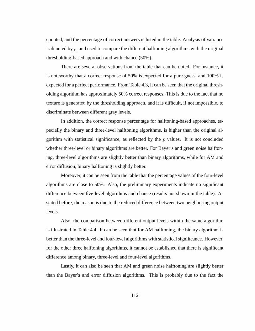
counted, and the percentage of correct answers is listed in the table. Analysis of variance

is denoted byp, and used to compare the different halftoning algorithms with the original

thresholding-based approach and with chance (50%).

There are several observations from the table that can be noted. For instance, it

is noteworthy that a correct response of 50% is expected for apure guess, and 100% is

expected for a perfect performance. From Table 4.3, it can beseen that the original thresh-

olding algorithm has approximately 50% correct responses.This is due to the fact that no

texture is generated by the thresholding approach, and it isdifficult, if not impossible, to

discriminate between different gray levels.

In addition, the correct response percentage for halftoning-based approaches, es-

pecially the binary and three-level halftoning algorithms, is higher than the original al-

gorithm with statistical significance, as reflected by thep values. It is not concluded

whether three-level or binary algorithms are better. For Bayer’s and green noise halfton-

ing, three-level algorithms are slightly better than binary algorithms, while for AM and

error diffusion, binary halftoning is slightly better.

Moreover, it can be seen from the table that the percentage values of the four-level

algorithms are close to 50%. Also, the preliminary experiments indicate no significant

difference between five-level algorithms and chance (results not shown in the table). As

stated before, the reason is due to the reduced difference between two neighboring output

levels.

Also, the comparison between different output levels within the same algorithm

is illustrated in Table 4.4. It can be seen that for AM halftoning, the binary algorithm is

better than the three-level and four-level algorithms withstatistical significance. However,

for the other three halftoning algorithms, it cannot be established that there is significant

difference among binary, three-level and four-level algorithms.

Lastly, it can also be seen that AM and green noise halftoningare slightly better

than the Bayer’s and error diffusion algorithms. This is probably due to the fact the

112

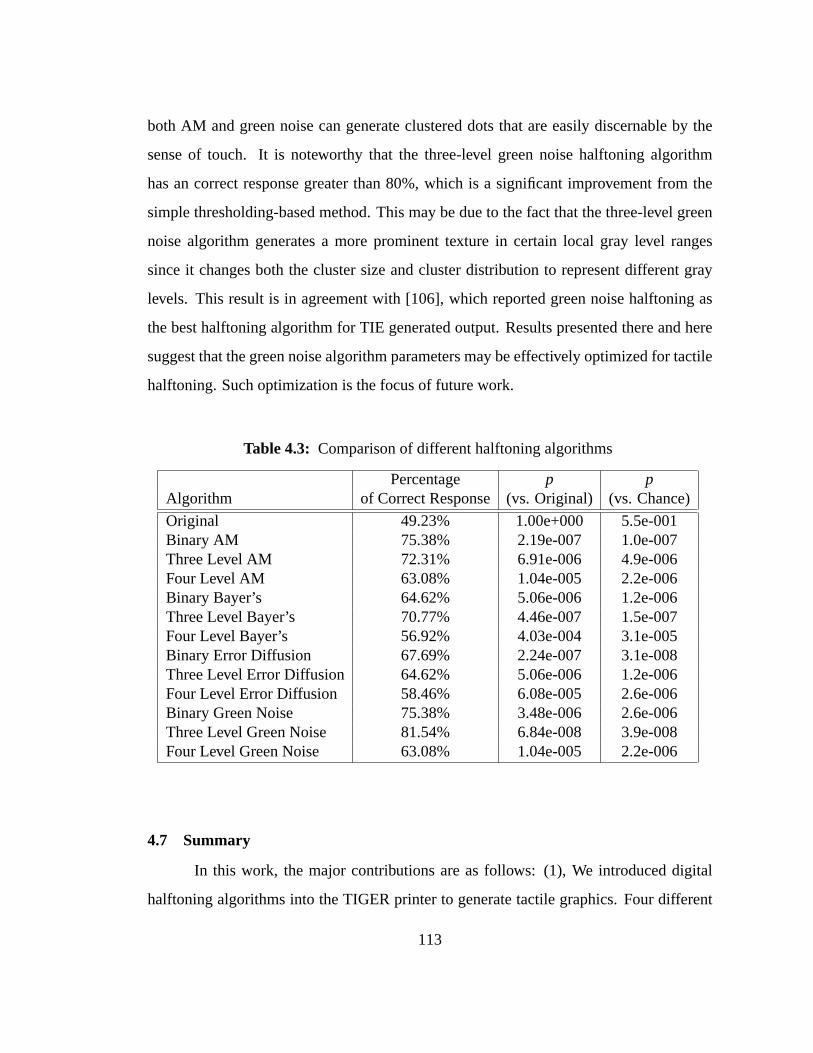
both AM and green noise can generate clustered dots that are easily discernable by the

sense of touch. It is noteworthy that the three-level green noise halftoning algorithm

has an correct response greater than 80%, which is a significant improvement from the

simple thresholding-based method. This may be due to the fact that the three-level green

noise algorithm generates a more prominent texture in certain local gray level ranges

since it changes both the cluster size and cluster distribution to represent different gray

levels. This result is in agreement with [106], which reported green noise halftoning as

the best halftoning algorithm for TIE generated output. Results presented there and here

suggest that the green noise algorithm parameters may be effectively optimized for tactile

halftoning. Such optimization is the focus of future work.

Table 4.3: Comparison of different halftoning algorithms

Percentage p pAlgorithm of Correct Response(vs. Original) (vs. Chance)

Original 49.23% 1.00e+000 5.5e-001Binary AM 75.38% 2.19e-007 1.0e-007Three Level AM 72.31% 6.91e-006 4.9e-006Four Level AM 63.08% 1.04e-005 2.2e-006Binary Bayer’s 64.62% 5.06e-006 1.2e-006Three Level Bayer’s 70.77% 4.46e-007 1.5e-007Four Level Bayer’s 56.92% 4.03e-004 3.1e-005Binary Error Diffusion 67.69% 2.24e-007 3.1e-008Three Level Error Diffusion 64.62% 5.06e-006 1.2e-006Four Level Error Diffusion 58.46% 6.08e-005 2.6e-006Binary Green Noise 75.38% 3.48e-006 2.6e-006Three Level Green Noise 81.54% 6.84e-008 3.9e-008Four Level Green Noise 63.08% 1.04e-005 2.2e-006

4.7 Summary

In this work, the major contributions are as follows: (1), Weintroduced digital

halftoning algorithms into the TIGER printer to generate tactile graphics. Four different

113

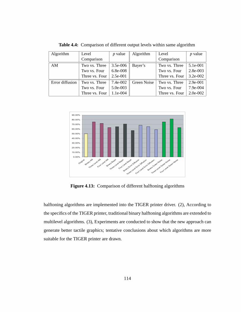
Table 4.4: Comparison of different output levels within same algorithm

Algorithm Level p value Algorithm Level p valueComparison Comparison

AM Two vs. Three 3.5e-006 Bayer’s Two vs. Three 5.1e-001Two vs. Four 6.8e-008 Two vs. Four 2.8e-003Three vs. Four 2.5e-001 Three vs. Four 3.2e-002

Error diffusion Two vs. Three 7.4e-002 Green Noise Two vs. Three 2.9e-001Two vs. Four 5.0e-003 Two vs. Four 7.9e-004Three vs. Four 1.1e-004 Three vs. Four 2.0e-002

0.00%

10.00%

20.00%

30.00%

40.00%

50.00%

60.00%

70.00%

80.00%

90.00%

Original

Binary

AM

Three

Leve

l AM

Four Lev

el AM

Binary

Baye

r

Three

Leve

l Bay

er

Four Lev

el Baye

r

Binary

Erro

r Diffu

sion

Three

Leve

l Erro

r Diff

usio

n

Four Lev

el Erro

r Diffu

sion

Binary

Gre

en Nois

e

Three

Leve

l Gre

en N

oise

Four Lev

el Gre

en Noise

Figure 4.13: Comparison of different halftoning algorithms

halftoning algorithms are implemented into the TIGER printer driver. (2), According to

the specifics of the TIGER printer, traditional binary halftoning algorithms are extended to

multilevel algorithms. (3), Experiments are conducted to show that the new approach can

generate better tactile graphics; tentative conclusions about which algorithms are more

suitable for the TIGER printer are drawn.

114

Chapter 5

CONCLUSIONS AND FUTURE DIRECTIONS

In this dissertation, we concentrated on performance optimization of three repre-

sentative applications from the bioinformatics or biomedical area using state-of-the-art

computer architectures and technologies. We believe the methodologies adopted in the

study of these three applications can be applied to other interesting applications as well.

First of all, we proposed a new task decomposition scheme to reduce data com-

munication and generated a scalable and robust cluster-based parallel Hmmpfam using

the EARTH (Efficient Architecture for Running Threads) model. The methodology is to

balance the computation and communication in cluster-based computing environments.

Secondly, we used the real biomedical application SPACE RIP asa context and

focused on the core algorithm SVD. We implemented the one-sided Jacobi parallel SVD

on Cyclops-64 to exploit the thread-level parallelism. We also developed a performance

model for the dissection of total execution cycles into fourparts and used this model to

compare different memory access approaches. We observed a significant performance

gain with the combination of these parallelization and optimization approaches.

Our work on the parallelization and optimization of SPACE RIP is one of the

attempts to adapt to the era of multicore processor designs.The new trend of multi-

core processors forces a fundamental change of software programming models. Many

applications have enjoyed free and regular performance gains for several decades, some-

times even without releasing new software versions and doing anything special, because

the CPU manufactures have enabled ever-faster mainstream systems. With the multi-

core processors, the “free lunch” is over [9]. Multithreaded software must be developed

115

to fully exploit the power of multicore processors. Moreover, efficiency and performance

tuning will get more important. With the results and conclusions from our optimization of

the SPACE RIP application, future extensions and optimizations to existing programming

languages and compilers may be developed.

Finally, we adapted different halftoning algorithms to a specific tactile printer and

conducted experiments to compare and evaluate them. The idea is to find a good way to

utilize modern computer technologies and image processingalgorithms to convert graph-

ics to multilevel halftoning texture patterns that are manually perceivable by individuals

with visual impairment. We concluded that the halftoning-based approach achieves sig-

nificant improvement in terms of its texture pattern discrimination ability and that the

green noise halftoning performs the best among different halftoning algorithms.

This dissertation shows the promise of using parallel computing technology and

digital imaging algorithms to find better solutions for realapplications. At the conclu-

sion of our research, we found that following areas have opened up for further explo-

ration. First of all, in the direction of combining bioinformatics/biomedical applications

and parallel computing, we may focus on other interesting and challenging applications.

Porting applications, such as multiple sequence alignment(MSA), to Cyclops-64 may

generate interesting findings, such as novel parallel schemes and insights for architecture

designs. Secondly, the current halftoning-based approachfor tactile graphics can be fur-

ther extended to process color images using digital color halftoning techniques. Digital

halftoning can also be integrated with other tactile imaging techniques, such as image

segmentation and edge detection, to generate the texture inthe segmented regions.

In conclusion, we feel that the combination of parallel computing and bioinfor-

matics/biomedical algorithm/applications is indeed an interesting multi-disciplinary area.

It is worthy to take long term efforts to develop innovative approaches and provide better

solutions to existing and emerging problems.

116

BIBLIOGRAPHY

[1] T. Sterling, D. Becker, and D. Savarese, “BEOWULF: A parallel workstation forscientific computation,”Proceedings of the 1995 International Conference on Par-allel Processing (ICPP), pp. 11–14, 1995.

[2] The 24th TOP500 Supercomputer List for Nov 2004. [Online]. Available:http://www.top500.org

[3] K. B. Theobald, “EARTH: An efficient architecture for running threads,” Ph.D.dissertation, McGill University, Montreal, 1999.

[4] H. H. J. Hum, O. Maquelin, K. B. Theobald, X. Tian, X. Tang, and G. R. G. et al.,“A design study of the EARTH multiprocessor,”Proceedings of the Conference onParallel Architectures and Compilation Techniques (PACT), pp. 59–68, 1995.

[5] T. Ungerer, B. Robic, and J.Silc, “A survey of processors with explicit multithread-ing,” ACM Comput. Surv., vol. 35, no. 1, pp. 29–63, 2003.

[6] G. R. Gao, L. Bic, and J.-L. Gaudiot, Eds.,Advanced Topics in Dataflow Com-puting and Multithreading. IEEE Comp. Soc. Press, 1995, book contains paperspresented at the Second Intl. Work. on Dataflow Computers, Hamilton Island, Aus-tralia, May 1992.

[7] S. J. Eggers, J. S. Emer, H. M. Levy, J. L. Lo, R. L. Stamm, andD. M. Tullsen,“Simultaneous multithreading: A platform for next-generation processors,”IEEEMicro, vol. 17, no. 5, pp. 12–19, 1997.

[8] G. A. Alverson, S. Kahan, R. Korry, C. McCann, and B. J. Smith, “Schedulingon the Tera MTA,” inIPPS ’95: Proceedings of the Workshop on Job SchedulingStrategies for Parallel Processing. London, UK: Springer-Verlag, 1995, pp. 19–44.

[9] H. Sutter, “The free lunch is over: A fundamental turn toward concurrency insoftware,”Dr. Dobb’s Journal, vol. 30, no. 3, March 2005. [Online]. Available:http://www.gotw.ca/publications/concurrency-ddj.htm

117

[10] C. Cascaval, J. G. C. nos, L. Ceze, M. Denneau, M. Gupta, D. Lieber, J. E. Moreira,K. Strauss, and H. S. W. Jr., “Evaluation of a multithreaded architecture for cellularcomputing,” inHPCA, 2002, pp. 311–322.

[11] G. Almai, C. Cascaval, J. G. Castanos, M. Denneau, D. Lieber, Jose E. Moreira,and J. Henry S. Warren, “Dissecting cyclops: a detailed analysis of a multithreadedarchitecture,”SPECIAL ISSUE: MEDEA workshop, vol. 31, pp. 26 – 38, 2003.

[12] G. S. Almasi, C. Cascaval, J. E. Moreira, M. Denneau, W. Donath, M. Elefthe-riou, M. Giampapa, H. Ho, D. Lieber, D. Newns, M. Snir, and J. Henry S. Warren,“Demonstrating the scalability of a molecular dynamics application on a petaflopcomputer,” inICS ’01: Proceedings of the 15th international conference onSuper-computing. New York, NY, USA: ACM Press, 2001, pp. 393–406.

[13] S. F. Altschul, W. Gish, W. Miller, E. W. Myers, , and D. J.Lipman, “A basic localalignment search tool,”Journal of Molecular Biology, vol. 215, p. 403C410, 1990.

[14] HMMER: sequence analysis using profile hidden Markov models. [Online].Available: http://hmmer.wustl.edu/

[15] V. S. Pande, I. B. 1, J. Chapman, S. P. Elmer, S. Khaliq, S. M.Larson, Y. M.Rhee, M. R. Shirts, C. D. Snow, E. J. Sorin, and B. Zagrovic, “Atomistic proteinfolding simulations on the submillisecond time scale usingworldwide distributedcomputing,”Biopolymers, vol. 68, no. 1, pp. 91–109, 2003.

[16] B. M. E. Moret, D. A. Bader, and T. Warnow, “High-performance algorithm en-gineering for computational phylogenetics,”J. Supercomput., vol. 22, no. 1, pp.99–111, 2002.

[17] C. Laurent, F. Peyrin, J.-M. Chassery, and M. Amiel, “Parallel image reconstruc-tion on MIMD computers for three-dimensional cone-beam tomography,”ParallelComputing, vol. 24, no. 9-10, pp. 1461–1479, 1998.

[18] S. K. Warfield, F. A. Jolesz, and R. Kikinis, “A high performance computing ap-proach to the registration of medical imaging data,”Parallel Computing, vol. 24,no. 9-10, pp. 1345–1368, 1998.

[19] G. E. Christensen, “MIMD vs. SIMD parallel processing: Acase study in 3d med-ical image registration.”Parallel Computing, vol. 24, no. 9-10, pp. 1369–1383,1998.

[20] M. Stacy, D. P. Hanson, J. J. Camp, and R. A. Robb, “High performance computingin biomedical imaging research,”Parallel Computing, vol. 24, no. 9-10, pp. 1287–1321, 1998.

118

[21] Wikipedia, the free encyclopedia. [Online]. Available:http://en.wikipedia.org/wiki/

[22] M. J. Flynn, “Some computer organizations and their effectiveness,”IEEE Trans.on Computers, vol. 21, no. 9, pp. 948–960, Sep. 1972.

[23] Barry Wilkinson and Michael Allen,Parallel Programming: Techniques and Ap-plications Using Networked Workstations and Parallel Computers, 1st ed. UpperSaddle River, New Jersey: Prentice Hall, August 12 1998.

[24] D. Culler, J. Singh, and A. Gupta,Parallel Computer Architecture : A Hardware/-Software Approach, 1st ed. San Francisco, CA: Morgan Kaufmann, August 11998.

[25] N. Adiga, M. Blumrich, and T. Liebsch, “An overview of theBlueGene/L super-computer,” inProceedings of the 2002 ACM/IEEE conference on Supercomputing,Baltimore, Maryland, 2002, pp. 1 – 22.

[26] A. Geist, A. Beguelin, J. Dongarra, W. Jiang, R. Manchek, and V. Sunderam,PVM:Parallel Virtual Machine – A Users’ Guide and Tutorial for Networked ParallelComputing. MIT Press, 1994.

[27] W. Gropp, E. Lusk, and A. Skjellum,Using MPI: Portable Parallel Programmingwith the Message-Passing Interface. Cambrdge, MA: MIT Press, Oct. 1994.

[28] S. Y. Borkar, P. Dubey, K. C. Kahn, D. J. Kuck, H. Mulder, S. S. Pawlowski,and J. R. Rattner, “Platform 2015: Intel processor and platform evolution forthe next decade,”Technology at Intel Magazine, 2005. [Online]. Available:http://www.intel.com/technology/magazine/computing/platform-2015-0305.htm

[29] D. A. Patterson and J. L. Hennessy,Computer architecture: a quantitative ap-proach. San Francisco, CA, USA: Morgan Kaufmann Publishers Inc., 1996.

[30] W. A. Wulf and S. A. McKee, “Hitting the memory wall: implications of the obvi-ous,”SIGARCH Comput. Archit. News, vol. 23, no. 1, pp. 20–24, 1995.

[31] D. R. Butenhof,Programming with POSIX(R) Threads. Addison-Wesley Pub.Co., 1997.

[32] P. Thulasiraman, “Irregular computations on fine-grain multithreaded architec-ture,” Ph.D. dissertation, University of Delaware, Newark, DE, 2000.

[33] J. B. Dennis and G. R. Gao, “Multithreaded architectures:Principles, projects, andissues,” inMultithreaded Computer Architecture: A Summary of the Stateof theArt, R. A. Iannucci, G. R. Gao, R. H. Halstead, Jr., and B. Smith, Eds. Norwell,

119

Mass.: Kluwer Academic Pub., 1994, ch. 1, pp. 1–72, book contains papers pre-sented at the Workshop on Multithreaded Computers, Albuquerque, N. Mex., Nov.1991.

[34] J. del Cuvillo, W. Zhu, Z. Hu, and G. R. Gao, “Fast: A functionally accurate sim-ulation toolset for the cyclops-64 cellular architecture,” in Workshop on Modeling,Benchmarking and Simulation (MoBS), held in conjunction with the 32nd AnnualInterantional Symposium on Computer Architecture (ISCA’05), Madison, Wiscon-sin, June 4 2005.

[35] ——, “Tiny threads: a thread virtual machine for the cyclops64 cellular architec-ture,” in Fifth Workshop on Massively Parallel Processing (WMPP), held in con-junction with the 19th International Parallel and Distributed Processing System,Denver, Colorado, April 3 - 8 2005.

[36] J.-L. Gaudiot and L. Bic, Eds.,Advanced Topics in Data-Flow Computing. En-glewood Cliffs, N. Jer.: Prentice-Hall, 1991, book containspapers presented at theFirst Workshop on Data-Flow Computing, Eilat, Israel, May 1989.

[37] J. von Neumann, “First draft of a report on the EDVAC,”IEEE Ann. Hist. Comput.,vol. 15, no. 4, pp. 27–75, 1993.

[38] R. A. Iannucci, “Toward a dataflow/von Neumann hybrid architecture,” inProc.of the 15th Ann. Intl. Symp. on Computer Architecture, Honolulu, Haw., May–Jun.1988, pp. 131–140.

[39] Platform 2015 Unveiled at IDF Spring 2005. [Online]. Available:http://www.intel.com/technology/techresearch/idf/platform-2015-keynote.htm

[40] J. Tisdall,Beginning Perl for Bioinformatics, 1st ed. Sebastopol, CA: O’Reilly,October 15 2001.

[41] The NCBI genebank statistics. [Online]. Available:http://www.ncbi.nlm.nih.gov/Genbank/genbankstats.html

[42] NCBI blast. [Online]. Available: http://www.ncbi.nlm.nih.gov/BLAST/

[43] M. Cameron, H. E. Williams, and A. Cannane, “Improved gapped alignment inblast,” IEEE/ACM Trans. Comput. Biol. Bioinformatics, vol. 1, no. 3, pp. 116–129,2004.

[44] C. A. Stewart, D. Hart, D. K. Berry, G. J. Olsen, E. A. Wernert, and W. Fischer,“Parallel implementation and performance of fastDNAml: a program for maximumlikelihood phylogenetic inference,” inSupercomputing ’01: Proceedings of the

120

2001 ACM/IEEE conference on Supercomputing (CDROM). New York, NY, USA:ACM Press, 2001, pp. 20–30.

[45] B. M. Moret, D. Bader, T. Warnow, S. Wyman, and M. Yan, “GRAPPA: a high-performance computational tool for phylogeny reconstruction from gene-orderdata,” inBotany 2001, Albuquerque, NM, August 12-16 2001.

[46] D. A. Bader, “Computational biology and high-performance computing,”Com-mun. ACM, vol. 47, no. 11, pp. 34–41, 2004.

[47] W. Zhu, Y. Niu, J. Lu, C. Shen, and G. R. Gao, “A cluster-based solution for highperformance hmmpfam using earth execution model,” inproceedings of Cluster2003, Hong Kong. P.R.China, December 1-4 2003, accepted to be published ina Special Issue of the International Journal of High Performance Computing andNetworking (IJHPCN).

[48] Y. Niu, Z. Hu, and G. R. Gao, “Parallel reconstruction forparallel imaging spacerip on cellular computer architecture,” inProceedings of The 16th IASTED Inter-national Conference on Parallel and Distributed Computing and Systems, Cam-bridge, MA, November 9-11, 2004.

[49] Y. Niu and K. E. Barner, “Generation of tactile graphics with multilevel digitalhalftoning,”IEEE transactions on Neural Systems and Rehabilitation Engineering,Oct 2004, submitted.

[50] D. W. Mount, Bioinformatics: Sequence and Genome Analysis, 1st ed. ColdSpring Harbor Laboratory Press, March 15 2001.

[51] J. T. L. Wang, Q. heng Ma, and C. H. Wu, “Application of neural network to bio-logical data mining: A case study in protein sequence classification,” Proceedingsof KDD-2000, pp. 305–309, 2000.

[52] T. K. Attwood, M. E. Beck, D. R. Flower, P. Scordis, and J. N.Selley, “ThePRINTS protein fingerprint database in its fifth year,”Nucleic Acids Research,vol. 26, no. 1, p. 304C308, 1998.

[53] S. Eddy, “Profile hidden markov models,”Bioinformatics, vol. 14, pp. 755–763,1998.

[54] A. Krogh, M. Brown, I. Mian, K. Sjolander, and D. Haussler, “Hidden markovmodels in computational biology: applications to protein modeling,” Journal ofMolecular Biology, vol. 235, pp. 1501–1531, 1994.

121

[55] P. Baldi, Y. Chauvin, T. Hunkapiller, and M. A. McClure, “Hidden markov modelsof biologicalprimary sequence information,”PNAS, vol. 91, no. 3, pp. 1059–1063,1994.

[56] S.E.Levinson, L.R.Rabiner, and M.M.Sondhi, “An introduction to the applicationof the theory of probabilistic functions of a markov processto automatic speechrecognition,”Bell Syst.Tech.J., vol. 62, pp. 1035–1074, 1983.

[57] P. Baldi and S. Brunak,Bioinformatics: The Machine Learning Approach, 2nd ed.Cambridge, MA: The MIT Press, August 1 2001.

[58] A. Bateman, E. Birney, L. Cerruti, R. Durbin, L. Etwiller, S.R. Eddy, S. Griffiths-Jones, K.L. Howe, M. Marshall, and E.L.L. Sonnhammer, “The pfam protein fam-ilies database,”Nucleic Acids Research, vol. 30, no. 1, pp. 276–280, 2002.

[59] E.L.L Sonnhameer, S.R. Eddy, and R. Durbin, “Pfam: A comprehensive databaseof protein domain families based on seed alignments,”Proteins, vol. 28, pp. 405–420, 1997.

[60] E.L.L Sonnhameer, S.R. Eddy, E. Birney, A. Bateman, and R. Durbin, “Pfam:Multiple sequence alignments and hmm-profiles of protein domains,”Nucl. AcidsRes., vol. 26, pp. 320–322, 1998.

[61] G. Tremblay, K. B. Theobald, C. J. Morrone, M. D. Butala, J. N. Amaral, andG. R. Gao, “Threaded-c language reference manual (release 2.0),” CAPSL Techni-cal Memo 39, 2000.

[62] C. J. Morrone, “An EARTH runtime system for multi-processor/multi-node Be-owulf clusters,” Master’s thesis, Univ. of Delaware, Newark, DE, May 2001.

[63] C. Li, “EARTH-SMP: Multithreading support on an SMP cluster,” Master’s thesis,Univ. of Delaware, Newark, DE, Apr. 1999.

[64] C. Shen, “A portable runtime system and its derivation for the hardware SU imple-mentation,” Master’s thesis, Univ. of Delaware, Newark, DE, December 2003.

[65] H. H. J. Hum, K. B. Theobald, and G. R. Gao, “Building multithreaded architec-tures with off-the-shelf microprocessors,”In Proceedings of the 8th InternationalParallel Processing Symposium, pp. 288–294, 1994.

[66] The Argonne Scalable Cluster. [Online]. Available: http://www-unix.mcs.anl.gov/chiba/

[67] The Argonne JAZZ Cluster, Laboratory Computing Resource Center (LCRC).[Online]. Available: http://www.lcrc.anl.gov/jazz/

122

[68] E. Anderson, Z. Bai, C. Bischof, S. Blackford, J. Demmel, J. Dongarra, J. Du Croz,A. Greenbaum, S. Hammarling, A. McKenney, and D. Sorensen,LAPACK Users’Guide, 3rd ed. Philadelphia, PA: Society for Industrial and Applied Mathematics,1999.

[69] J. B. del Cuvillo, Z. Hu, W. Zhu, F. Chen, and G. R. Gao, “CAPSL memo 55:Toward a software infrastructure for the cyclops64 cellular architecture,” CAPSLGroup, Department of ECE, University of Delaware, Tech. Rep.,2004.

[70] D. W. McRobbie, E. A. Moore, M. J. Graves, and M. R. Prince,MRI from Pictureto Proton. Cambridge University Press, December 5 2002.

[71] R. B. Buxton,Introduction to Functional Magnetic Resonance Imaging : Princi-ples and Techniques. Cambridge University Press, November 2001.

[72] P. Woodward,MRI for Technologists. McGraw-Hill Companies, October 2000.

[73] Pruessmann KP, Weiger M, Boernert P, and Boesiger P, “SENSE, sensitivity en-coding for fast MRI,”Magn Reson Med, vol. 42, pp. 952–962, 1999.

[74] D. Atkinson, “Parallel imaging reconstruction,” inWorkshop on Image Process-ing for MRI, held in conjunction with The 2004 British Chapter ISMRM meeting,Edinburgh, UK, September 2004.

[75] Sodickson DK and Manning WJ, “Simultaneous acquistion of spatial harmon-ics(SMASH): fast imaging with radiofrequency coil arrays,” Magn Reson Med,vol. 38, no. 4, pp. 591–603, 1997.

[76] Kyriakos WE, Panych LP, Kacher DF, Westin C-F, Bao SM, Mulkern RV, andJolesz FA, “Sensitivity profiles from an array of coils for encoding and reconstruc-tion in parallel (SPACE RIP),”Magn Reson Med, vol. 44, no. 2, pp. 301–308, 2000.

[77] R. Chandra, R. Menon, L. Dagum, D. Kohr, D. Maydan, and J. McDonald,ParallelProgramming in OpenMP. Morgan Kaufmann, 2000.

[78] G. R. Gao and S. J. Thomas, “An optimal parallel jacobi-like solution method forthe singular value decomposition,” inProc. Internat. Conf. Parallel Proc., 1988,pp. 47–53.

[79] M. Gu, J. Demmel, and I. Dhillon, “Efficient computationof the singular value de-composition with applications to least squares problems,”Computer Science Dept.,University of Tennessee, Knoxville, Tech. Rep. CS-94-257, 1994, LAPACK Work-ing Note 88, http://www.netlib.org/lapack/lawns/lawn88.ps.

123

[80] L. S. Blackford, J. Choi, A. Cleary, E. D’Azevedo, J. Demmel, I. Dhillon, J. Don-garra, S. Hammarling, G. Henry, A. Petitet, K. Stanley, D. Walker, and R. C. Wha-ley, ScaLAPACK Users’ Guide. Philadelphia, PA: Society for Industrial and Ap-plied Mathematics, 1997.

[81] J. Demmel,Applied Numerical Linear Algebra. SIAM, 1997.

[82] G. Golub and C. V. Loan,Matrix Computations. The Johns Hopkins UniversityPress, Baltimore, 1996.

[83] J. Demmel, M. Gu, S. Eisenstat, I. Slapnicar, K. Veselic, and Z. Drmac, “Comput-ing the singular value decomposition with high relative accuracy,”Linear AlgebraAppl., vol. 299, pp. 21–80, 1999.

[84] J. Demmel, “Accurate SVDs of structured matrices,”SIAM J. Matrix Anal. Appl.,vol. 21, no. 3, pp. 562–580, 2000.

[85] J. Demmel and K. Veselic, “Jacobi’s method is more accurate than QR,”October 1989, lapack Working Note 15 (LAWN-15), Available from netlib,http://www.netlib.org/lapack/.

[86] M. R. Hestenes, “Inversion of matrices of biorthogonalization and related results,”J. Soc. Induct. Appl. Math., vol. 6, pp. 51–90, 1958.

[87] H. Rutishauser, “The jacobi method for real symmetric matrices,” inJ. H. Wilkin-son and C. Reinsch, editors, Linear Algebra, Volumn II of Handbook for AutomaticComputations, chapter II/1, vol. II, 1971, pp. 202–211.

[88] H. Park, “A real algorithm for the hermitian eigenvaluedecomposition,”BIT,vol. 33, pp. 158–171, 1993.

[89] G. E. Forsythe and P. Henrici, “The cyclic jacobi methodfor computing the prin-cipal values of a complex matrix,”Transactions of the American MethematicalSociety, vol. 94, no. 1, pp. 1–23, 1960.

[90] R. P. Brent and F. T. Luk, “The solution of singular-value and symmetric eigenvalueproblems on multiprocessor arrays,”SIAM Journal on Scientific and StatisticalComputing, vol. 6, no. 1, pp. 69–84, January 1985.

[91] R. P. Brent, F. T. Luk, and Charles F. Van Loan, “Computation of the singular valuedecomposition using mesh-connected processors,”Journal of VLSI and ComputerSystems, vol. 1, no. 3, pp. 242–260, 1985.

[92] D. Royo, M. Valero-Garcıa, and Antonio Gonzalez, “Implementing the one-sidedjacobi method on a 2D/3D mesh multicomputer,”Parallel Computing, vol. 27,no. 9, pp. 1253–1271, August 2001.

124

[93] E. R. Hansen, “On cyclic jacoib methods,”Journal of Soc. Indust. Appl. Math.,vol. 11, pp. 448–459, 1963.

[94] J. H. Wilkinson, The Algebraic Eigenvalue Problem, pp. 277-278. Oxford:Clarendon Press, 1965.

[95] S. Coren and L. Ward,Sensation and Perception (3rd Edition). San Diego, Cali-fornia: Harcout Brace Jovanovich, 1989.

[96] ALVA Access Group Homepage. [Online]. Available: http://www.aagi.com/

[97] B. Lowenfield,The Changing Status of the Blind: From Separations to Integration.Springfield, Illinois: Charles C. Thomas, 1975.

[98] J. Bliss, “A relatively high-resolution reading aid forthe blind,” IEEE Transactionson Man-Machine Systems, vol. 10, no. 1, pp. 1–9, 1969.

[99] M. Kurze, L. Reichert, and T. Strothotte, “Access to business graphics for blindpeople,” in Proceedings of the RESNA’94 Annual conference, Nashville, Ten-nessee, June 17-22 1994.

[100] T. P. Way and K. E. Barner, “Automatic visual to tactile translation, part I: Humanfactors, access methods and image manipulation,”IEEE Transactions on Rehabil-itation Engineering, vol. 5, no. 1, pp. 81–94, March 1997.

[101] ——, “Automatic visual to tactile translation, part II: Evaluation of the tactile im-age creation system,”IEEE Transactions on Rehabilitation Engineering, vol. 5,no. 1, pp. 95–105, March 1997.

[102] S. Hernandez and K. E. Barner, “Joint region merging criteria for watershed-basedimage segmentation,” inInternational Conference on Image Processing, Vancou-ver, BC, Canada, September 10-13 2000.

[103] ——, “Tactile imaging using watershed-based image segmentation,” inProceed-ings of the fourth international ACM conference on Assistivetechnologies, Arling-ton, Virginia, November 13-15 2000, pp. 26 – 33.

[104] S. Hernandez, K. E. Barner, and Y. Yuan, “Region merging using region homo-geneity and edge integrity for watershed-based image segmentation,” Optical En-gineering, July 2004, accepted for publication.

[105] Repro-Tronics Homepage. [Online]. Available: http://www.repro-tronics.com/

[106] A. Nayak and K. E. Barner, “Optimal halftoning for tactile imaging,”IEEE Trans-actions on Neural Systems and Rehabilitation Engineering, vol. 12, no. 2, pp. 216–227, June 2004.

125

[107] R. A. Ulichney,Digital Halftoning. Cambridge, MA: MIT Press, 1975.

[108] D. L. Lau,Modern Digital Halftoning. New York, NY: Marcel Dekker, 2000.

[109] H. R. Kang,Digital Color Halftoning. New York, NY: IEEE Press, 2000.

[110] B. E. Bayer, “An optimum method for two level rendition ofcontinuous-tone pic-tures,” in IEEE International Conference on Communications, Seattle, Washing-ton, June 11-13 1973, pp. 11–15.

[111] R. W. Floyd and L. Steinberg, “An adaptive algorithm forspatial gray-scale,” inProceedings Society Information Display, vol. 17, February 1976, pp. 75–77.

[112] R. Levien, “Output dependant feedback in error diffusion halftoning,” inIS&T’sEighth International Congress on Advances in Non-Impact Printing Technologies,Willianmsburg, Virginia, October 25-30 1992, pp. 280–282.

[113] American Thermoform Corporation Homepage. [Online].Available:http://www.atcbrleqp.com/swell.htm

[114] Pulse Data International Homepage. [Online]. Available:http://www.pulsedata.co.nz

[115] ViewPlus Technologies. [Online]. Available: http://www.viewplustech.com

[116] S. Ellwanger and K. E. Barner, “Tactile image conversion and printing,” IEEETransactions on Neural Systems and Rehabilitation Engineering, August 2004,submitted for publication.

[117] K. O. Johnson and J. R. Phillips, “Tactile spatial resolution: Two-point discrimi-nation, gap detection, grating resolution, and letter recognition,” Journal of Neuro-physiology, vol. 46, no. 6, 1981.

[118] J. Sullivan, L. Ray, and R. Miller, “Design of minimum visual modulation halftonepatterns,”IEEE Transactions on Systems, Man and Cybernetics, vol. 21, no. 1, pp.33–38, Jan/Feb 1991.

[119] M. Rodriguez, “Graphic arts perspective on digital halftoning,” in Proceedings ofSPIE, Human Vision, Visual Processing and Digital Display V, B. E. Rogowitz andJ. P. Allebach, Eds., vol. 2179, Feb 1994, pp. 144–149.

[120] J. F. Jarvis, C. N. Judice, and W. H. Ninke, “A survey of technique for the displayof continuous-tone pictures on bilevel displays,”Computer Graphics and ImageProcessing, vol. 5, no. 1, pp. 13–40, 1976.

126

[121] P. Stucki, “Mecca-a multiple-error correcting computation algorithm for bilevelimage hardcopy reproduction,” RZ 1060 IBM Research Laboratory, Zurich,Switzerland, Tech. Rep., 1981.

[122] T. S. Hang, “PCM picture transmission,”IEEE Spectrum, vol. 2, no. 12, pp. 57–63,1965.

[123] R. S. Gentile, E. Walowit, and J. P. Allebach, “Quantization and multilevel halfton-ing of color images for near original image quality,”Journal of the Optical Societyof America A, vol. 7, no. 6, pp. 1019–1026, 1990.

[124] K.E.Spaulding, R.L.Miller, and J. Schildkraut, “Methods for generating blue-noisedither matrices for digital halftoning,”Journal of Electronic Imaging, vol. 6, no. 3,pp. 208–230, 1997.

[125] F. Faheem, D. L. Lau, and G. R. Arce, “Digital multitoning using gray level separa-tion,” The Journal of Imaging Science and Technology, vol. 46, no. 5, pp. 385–397,September 2002.

[126] Microsoft Corporation, Ed.,Microsoft Windows 2000 Driver Development Kit.Microsoft Press, April 2000.

[127] B. Lowenfeld, “Effects of blindness on the cognitive functions of children,” inBerthold Lowefeld on Blindness and Blind People, B. Lowenfeld, Ed. AmericanFoundation for the Blind, 1981.

[128] T. P. Way, “Automatic generation of tactile graphics,” Master’s thesis, Universityof Delaware, Newark, DE, Fall 1996.

127