See discussions, stats, and author profiles for this publication at: https://www.researchgate.net/publication/340731400

A Novel Hyperspectral Anomaly Detection Algorithm for Real Time Applications

with Push-broom Sensors

Preprint · April 2020

CITATIONS

0READS

17

6 authors, including:

Some of the authors of this publication are also working on these related projects:

ENABLE-S3 View project

ADRES/DRESC View project

Pablo Horstrand

Universidad de Las Palmas de Gran Canaria

16 PUBLICATIONS   87 CITATIONS   

SEE PROFILE

Maria Diaz

Universidad de Las Palmas de Gran Canaria

18 PUBLICATIONS   59 CITATIONS   

SEE PROFILE

Raul Guerra Hernández

IUMA

31 PUBLICATIONS   176 CITATIONS   

SEE PROFILE

Sebastian Lopez

Universidad de Las Palmas de Gran Canaria

133 PUBLICATIONS   930 CITATIONS   

SEE PROFILE

All content following this page was uploaded by Pablo Horstrand on 18 April 2020.

The user has requested enhancement of the downloaded file.

1

A Novel Hyperspectral Anomaly DetectionAlgorithm for Real Time Applications with

Push-broom SensorsPablo Horstrand, María Díaz, Raúl Guerra, Sebastián López, Member, IEEE, and José Fco. López

Abstract—Most practical hyperspectral anomaly detection(AD) applications require real-time processing for detectingcomplex targets from their background. This is especially criticalin defense and surveillance domains, but also in many otherscenarios in which a rapid response is mandatory to save humanlives. Dealing with such a high dimensionality of data requires theconception of new algorithms to ease the demanding computingperformance. Push-broom scanning represents the mainstreamin hyperspectral imaging, introducing added complexity to theequation as there is no information of future pixels. In thispaper a novel technique named Line-by-line Anomaly Detection(LbL-AD) algorithm, is presented as a way of performing real-time processing with a push-broom sensor. The sensor has beenmounted on an unmanned aerial vehicle (UAV), and the acquiredimages, together with others from the scientific literature and syn-thetic ones, have been used to extensively validate the proposedalgorithm in terms of accuracy, based on different metrics, andprocessing time. Comparisons with state-of-the-art algorithmswere accomplished in order to evaluate the goodness of the LbL-AD, giving as a result an outstanding performance.

Index Terms—anomaly detection; unmanned aerial vehicle;push-broom sensor; hyperspectral imagery; onboard processing

I. INTRODUCTION

THE use of unmanned aerial vehicles (UAVs) equippedwith multi/hyperspectral sensors has gained momentum

in the last few years as a smart strategy for collecting datafor inspection, surveillance and monitoring in the areas ofdefense, security, environmental protection and civil domains,among others. The advantages of these aerial platforms overEarth Observation satellites or manned airborne platforms isthat they represent a lower-cost approach with a more flexiblerevisit time, while providing better spatial and sometimes evenbetter spectral imagery resolutions, which permits a deeper anda more accurate data analysis [1].

There are several applications that benefit from these aerialplatforms. For instance in the agriculture domain, the utiliza-tion of UAVs for the acquisition of remotely sensed data hasexperienced an exponential growth [2], due to their capacityof periodically monitoring the state of the crops, their growth,ground water content and other valuable information for the

This work has been supported by the European Commission through theECSEL Joint Undertaking (ENABLE-S3 project, No. 692455), the SpanishGoverment through the projects ENABLE-S3 (No. PCIN-2015-225) andPLATINO (No. TEC2017-86722-C4-1-R) and the Agencia Canaria de Investi-gación, Innovación y Sociedad de la Información (ACIISI)" of the "Conserjeríade Economía, Industria, Comercio y Conocimiento" of the "Gobierno deCanarias", which is part-financed by the European Social Fund (FSE) (POC2014-2020, Eje 3 Tema Prioritario 74 (85%).

farmers, potentially increasing productivity and decreasingthe costs. This application shares a common pattern withmany others that also make use of UAV platforms withmulti/hyperspectral sensors: images are first captured, thendata are downloaded after the flight is completed, and finallydata are processed offline to provide a result hours or evendays later.

Nevertheless, there exist other applications in which aprompt response is mandatory. This is the case of the ap-plication motivating this work, which is a particular use casewithin the European H2020 project ENABLE-S3 (EuropeanInitiative to Enable Validation for Highly Automated Safeand Secure Systems). The goal for this particular scenariois the automated driving of a harvester in an agriculturalfield performing the cropping, watering or pesticide sprayingtasks. Initially, a drone equipped with a hyperspectral camerainspects the terrain in order to generate a set of maps withdifferent vegetation indices which gives information relatedto the status of the crop. This information, together withthe specific coordinates, is then sent to the harvester, whichinitiates its autonomous driving to the region of interest andstarts its labour. In relation with this driving activity, muchhas been reported related to fatal accidents due to agriculturalmowing operations which injure or kill animals. Additionally,any collision with a big obstacle (animal or rock) means arepairing cost which in some cases could be prohibitive. Inorder to avoid these situations and promote a wildlife friendlyagro operation, a scheme similar to the one shown in Figure1 is depicted. The drone flies at an altitude, h, and somemeters ahead of the harvester (security distance), whichdepends on the harvester speed. If the hyperspectral cameradetects an obstacle, a stop&go signal is sent to the harvester,and depending on the characteristic of the obstacle (dynamicor static) the harvester will stop till the dynamic obstacledisappears, or start an avoidance maneuver if it is static.

The presented scenario entails some major challenges thatare not overlooked by the authors and need to be further de-tailed. For instance, it is well known that the current autonomyof commercial UAV solutions powered by batteries is in theorder of tens of minutes making the whole operation too dis-continuous and therefore unattractive for potential users. Thereare nonetheless works in the scientific literature proposingdifferent solutions for such problem. On one hand, a wirelesspower charge approach in order to reduce the stopping time[3]. On the other hand the use of alternative propulsion systems(or hybrid combinations of some of them), which alleviate the

2

restrictions imposed by electric batteries in terms of autonomy,are attracting great attention from the scientific community[4][5][6]. Another important aspect to take into account whenit comes to UAVs, being an autonomous vehicle, is the safetycritical operation it implies. Regulations are rather strict andsometimes even present an additional economical burden.However, as we see in other domains such as fire monitoring[7], construction hazards [8], or even photogrammetry underextreme weather conditions [9], the safety operation can bekept and at the same time profit the advantages of the use ofsuch system

There are different strategies that have been evaluated tosort the problematic raised by the ENABLE-S3 Farming UseCase presented before, mainly based on thermal sensors [10]and LIDARs. When implementing such autonomous vehicletechnologies, being at stake animals and human being lives,safety and security becomes a critical issue and therefore, theright approach is the combination of different technologies.Thermal approach may fail in warm environments where livingbeings are not so well distinguish anymore, and of course aswell detecting inert objects. On the other hand, LIDARs, mightbe alternatively installed in the harvesting vehicle or in thesupervisory drone. When mounted on the harvester, an uneventerrain profile or the height of the crop can produce falsepositives, while mounting it on the drone has the drawbackof additional weight and power consumption, reducing thewhole system autonomy. In this sense, great effort has beencarried out by the scientific community to reduce the sensorweight [11][12]. For the mentioned reasons, a new approach,is proposed in this work, consisting in using hyperspectralimages (HSIs) that could complement the results obtainedby the mentioned technologies. Since we are dealing witha homogeneous field with small objects coming up in thescene from time to time, anomaly detection (AD) has beenselected as an alternative approach to tackle the problem. Suchtechnique applied to hyperspectral data allows distinguishingrare objects with unknown spectral signatures that are not par-ticularly abundant in a scene. This possibility of distinguishinga scarce group of pixels whose spectral signature significantlydiffers from their surroundings represents a crucial feature andhas inspired the appearance of a huge amount of hyperspectralAD algorithms in the recent scientific literature.

The Reed-Xiaoli (RX) algorithm [13] is one of the firstdevelopments in this field, being viewed as a benchmarkto which other methods are compared. The RX anomalydetector is based on the Mahalanobis distance between thepixel under test and the background class. It assumes thatthe background follows a single Gaussian normal distributionand the probability density function is used to classify pixelsas part of the background class. Thus, the background meanand the inverse covariance matrix must be well estimated;otherwise, they could be contaminated by anomalies causinga subsequent misclassification. Several variations of the RXdetection technique have been proposed in the literature inorder to improve its performance. Subspace RX (SSRX) [14]and RX after orthogonal subspace projection (OSPRX) [15]are global anomaly detectors that apply principal componentanalysis (PCA) or singular value decomposition (SVD) to the

datacube. The goal is to reduce the data volume to a smallersubspace where the first PCA/SVD bands are supposed torepresent the background class. SSRX discards these bands,and then, RX is applied to the remaining subspace. Onthe contrary, OSPRX projects the data onto the orthogonalsubspace before applying RX.

In the recent years, new approaches to the problemhave emerged, in order to cope, for instance, with inad-equate Gaussian-distributed representations for nonhomoge-neous backgrounds [16], the presence of noise in the images,by using a combined similarity criterion anomaly detector(CSCAD) method [17], as well as the removal of outliers byusing a collaborative representation detector (CRD) [18][19].Other authors have explored techniques extensively used inother machine vision domains as it is the use of dictionaries,to separate the anomalies from the background [20], and evencombined the anomaly detection process with another verycommon processing stage in HSI such as compression [21].

stop

&go

signa

l

h

drone speed

harvester speed

(a)

Fig. 1: Automated harvesting process, with the UAV a fewmeters in front of the harvester scanning the field ahead forobstacle detection.

Unfortunately, all these algorithms require the sensing of thewhole hyperspectral image before starting with the process offinding the anomalies in the captured scene. However, the mostwidely used sensors in nowadays remote sensing applicationsare based on push-broom hyperspectral scanners, in which theimage is captured in a line-by-line fashion, since they providean outstanding spectral resolution and take advantage of themovement of the UAV, aircraft or satellite that carries them forcapturing the whole hypercube. Hence, for applications understrict real-time constraints in which the captured images mustbe processed in a short period of time, it is more efficientif the anomalies are uncovered as soon as the hyperspectral

3

data are sensed. Moreover, this kind of on-the-fly anomalydetection drastically reduces the vast amount of memory thatis required on-board the sensing platform in order to store theentire hypercubes.

In this scenario, this paper proposes a novel hyperspectralanomaly detection algorithm specially conceived for beingable to process the lines of pixels captured by a push-broomscanner as soon as they are sensed. More concretely, theproposed Line-by-Line Anomaly Detection (LbL-AD) algo-rithm is based, similar to the OSPRX algorithm, on theconcept of orthogonal subspace projections but employing alow computational processing chain that guarantees a precisedetection of the anomalies present in a hyperspectral scene.

For the purpose of testing the performance of the algorithmpresented in this paper, synthetic images as well as real imagescaptured both by commercial aerial platforms and by our ownUAV platform based on a Specim FX10 VNIR hyperspectralpush-broom sensor [22] mounted on a DJI Matrice 600 drone[23], have been used.

The rest of the paper is organized as follows. Section II de-scribes, step by step, the proposed LbL-AD algorithm. SectionIII presents the hyperspectral data and the assessment metricsutilized for comparing the performance given by the LbL-AD algorithm versus other state-of-the-art proposals. SectionIV outlines the main results obtained in terms of detectionperformance and execution performance. Finally, Section Vdraws the most representative conclusions achieved in thiswork as well as further research directions.

II. THE LBL-AD ALGORITHM

As it has been already mentioned, the LbL-AD algorithmis an anomaly detection algorithm suitable for real-time appli-cations using push-broom hyperspectral sensors whose mainadvantage is its fast computation combined with a gooddetection performance, being able to process each line ofpixels as soon as they are sensed. This implies a reductionin the required memory resources since it is not necessary tostore the full hypercube prior to its processing.

In order to keep a low computational complexity of theanomaly detection process, the proposed LbL-AD algorithmfollows a twofold strategy: it starts processing as a wholebunch the first n lines captured and then it follows a pro-gressive line-by-line processing for the rest of the lines ofthe image in which only a reduced amount of operations areperformed in order to update the results for the new acquiredline of pixels.

In particular, the following procedure is carried out for thefirst n lines captured by the sensor:

1) A reference average pixel is computed considering all thepixels contained in these lines.

2) The previously obtained average value is subtracted toeach sensed pixel.

3) The covariance matrix corresponding to these pixels iscalculated. At this point, it is worth to highlight that thiscovariance matrix is not divided by the total number ofpixels, since in this way this matrix can be reutilized inthe next iterations (next lines of pixels), adding to it the

new covariance matrix of the acquired line. For this towork, the number of pixels so far processed needs to beaccounted as well.

4) Principal component analysis is performed then onto thecovariance matrix to find the d highest eigenvalues andtheir associated eigenvectors. Here, in order to keep theLbL-AD algorithm within a low computational burden,the following computing strategy is applied:

a) First, the highest eigenvalue and its associated eigen-vector are obtained by means of the power iterationmethod [24].

b) Afterwards, deflation [25] is performed onto the co-variance matrix to calculate the next d− 1 eigenvaluesand eigenvectors, by means of successively applyingthe power iteration method. This process is repeateduntil the d desired number of components is obtained.

The reason for having selected this combination of meth-ods is dual: on one hand, it is a very fast method forjust obtaining a few principal components, and on theother hand, if the algorithm is wisely initialized, thecomputation time can be significantly reduced. This lastcharacteristic is exploited by the proposed LbL-AD algo-rithm, as for each iteration (each new line of pixels thatis acquired after the first n lines) the subspace calculatedfrom the previously sensed pixels is used for initializingthe algorithm, which brings a significant speedup factorto the process.

5) The pixels are projected onto the subspace spanned bythe d eigenvectors obtained in the previous step.

6) The Mahalanobis distance is calculated for each pixel, asit is done in the original RX algorithm. This step involvesthe calculation of the pseudoinverse of the covariancematrix. However, as far as the covariance matrix in thenew projected subspace is a diagonal matrix, its inverse isobtained by just inverting its single elements individually,which is again a huge save in terms of computing time.

7) Based on the calculated distance result, it is decidedwhether each pixel is an anomaly or not. Thanks to thegood separability between background and anomalies ofthe result provided by the algorithm, this task is carriedout applying a simple technique of outlier detection.

8) The background pixels Mahalanobis distance mean valueand standard deviation are computed for later use in theprocess.

Once these n lines of pixels have been processed thefollowing line-by-line procedure is carried out for the rest ofthe pixels in the hyperspectral scene under analysis:

A. The average pixel obtained previously in step 1 is sub-tracted to each pixel of the line under processing.

B. The covariance matrix of the line under processing iscalculated and added to the existing covariance matrixcalculated previously in step 3. As with step A, this isperformed under the assumption that the average pixelobtained in step 1 remains approximately constant, whichallows to skip the full computation of a new covariancematrix for each new line of pixels. Moreover, this methodallows us to keep in memory just the previous covariance

4

matrix, but not the entire amount of pixels processed,which means a huge save in memory space and numberof memory transactions.

C. Steps 4 to 7 are applied to the line of pixels underprocessing.

D. If in step 7, anomalies were detected, then the recentlycalculated covariance matrix is discarded, and the previ-ous covariance matrix available recovered for processingthe next line. The reason for doing this is to keep asmuch as possible the covariance matrix modeling onlythe background, so whenever an anomaly is coming intothe scene it will be something new. This confides theresult an homogeneity that otherwise it would not have.

E. Finally, previous step 8 is applied, exclusively to thebackground pixels.

Figure 2 shows a general vision of the stages involved inthe described algorithm. The following subsections will detailthe different parts of the proposed algorithm.

Buffer n lines

HSI frame

Obtain eigenvalues & eigenvectors

Project Image into new subspace

Obtain Mahalanobis distance of each pixel

Update Σ

i < ni < n

i = n

Pro

cess

the f

rst

n lin

es

i > n

µCalculate µ

Calculate Σ

Select Σ for next iteration

Σ

Fig. 2: General overview of the LbL-AD algorithm.

A. Computation of first n lines

The first n lines are buffered into a matrix, M , whichafterwards is used to calculate the average pixel, µ, to besubstracted to every processed image line. The covariancematrix, Σ, results from the obtained normalized matrix M ′,for which the eigenvectors, ~u1, ..., ~ud, and the eigenvalues,s1, ..., sd, are calculated. After that, the new subspace iscalculated as explained in the next subsection. Algorithm 1

shows the pseudocode of the algorithm initialization, where rstands for each captured line of nc pixels.

Algorithm 1: Computation of first n linesInputs: M = [r1, r2, ..., rn] where ri = [si1, si2, ..., sinc];

{Initial portion of the HSI}d, {Number of principal components to be selected}N = n× nc, {Number pixels contained in the first nlines}

P.1 µ = mean(M); {Average pixel}P.2 for i = 1 to n doP.3 for j = 1 to nc doP.4 sij = sij − µ;P.5 endP.6 endP.7 Σ = MTM;

P.8 M’ =Σ

N;

P.9 [Psi, S] = PCA(M’,d);Outputs:Σ, {Covariance matrix}S, {Eigenvalues}PSI, {Eigenvectors}n, {Number of processed pixels}µ, {Average pixel}

B. Subspace calculation. Power Iteration method and defla-tion.

On the first run the subspace is calculated for the computedcovariance matrix, Σ, from the buffered n lines and then itis updated on each iteration after the covariance matrix hasbeen updated. Since in the first iteration there are no previouseigenvectors for feeding the algorithm, the input eigenvectors,PSIin, are initialized with random values. However, on thesubsequent iterations the set of eigenvectors defining theprevious subspace are introduced as inputs of the algorithmand used to initialize the calculation, considering that thereshall not be a big difference between the set of eigenvectorscomputed from two consecutive iterations. The other twoinputs to the algorithm are the number of eigenvalues andeigenvectors to be calculated, d, and a stop condition for theconvergence of the power iteration method, tol. An auxiliarymatrix, B, is used to deflate the original covariance matrix andkeep calculating subsequent eigenvalues and eigenvectors. Thedeflation process mainly consists in obtaining a new matrixthat provides the same result than the original one in theorthogonal direction to it and it is zero otherwise. A detaileddescription of the subspace calculation process is presented inAlgorithm 2.

The subspace algorithm makes a recurrent call to thePower Method function, whose behavior is described inAlgorithm 3, until all d eigenvalues and eigenvectors havebeen obtained. As explained earlier, the initialization with theprevious obtained eigenvector is used to speed up convergence,which combined with the use of the Rayleigh coefficient,rayl, has proven to be very efficient [26]. This coefficient is

5

Algorithm 2: Subspace calculationInputs: Σ, {Covariance matrix}PSIin, {Input Eigenvectors }d, {number of eigenvalues to be calculated}tol, {stop condition for the power iteration method}

P.1 [PSI1, S1] = power method(Σ, tol, PSI_in1);P.2 i = 2;P.3 B = Σ; {Support matrix to compute deflation}P.4 while i <= d doP.5 B = B− PSITi−1PSIi−1;P.6 [PSIi, Si] = powermethod(Σ, tol, PSI_ini);P.7 i = i + 1;P.8 end

Outputs:S, {Eigenvalues}PSI, {Eigenvectors }

calculated using the eigenvector approximation and representsin its turn a very good approximation of the eigenvalue. Themethod consists in iteratively calculating the new coefficient,rayl, with the recently obtained vector and comparing it withthe value calculated in the previous iteration, rayl0, until thedifference between them is lower than the input tolerance, tol.

Algorithm 3: Power MethodInputs: Σ, {Covariance matrix}bk, {Input Eigenvector}tol, {stop condition}

P.1 rayl0 = 0;

P.2 rayl =bTk Σbk

bTk bk

;P.3 while abs(rayl0 − rayl) > tol doP.4 rayl0 = rayl;P.5 bk+1 = Σbk

‖Σbk‖ ;

P.6 rayl =bTk Σbk

bTk bk

;P.7 end

Outputs:rayl, {Calculated Eigenvalue}bk, {Calculated Eigenvector}

C. Image Projection and Distance Calculation

After the first n lines have been processed, the proposedalgorithm processes the sensed data line by line, as it isdescribed in Algorithm 4. As it has been already mentioned,the average pixel, µ, obtained in the first stage of the algorithm,is substracted from each pixel, and then, the covariance matrixis updated to obtain Σnew and the new set of d eigenvaluesand eigenvectors from the updtaed Σnew. The process thencontinues projecting the image onto the new subspace andobtaining the Mahalanobis distance for each pixel. Finally,the mean value, µdist, and the standard deviation, σdist, ofthe Mahalanobis distance of just the background pixels arecalculated and updated on every iteration, in order to accountfor possible outliers, and thus, anomalies. In case anomalies

are found, the covariance matrix of the previous iteration isused, instead of the updated one as long as it is not the firstiteration. As it can be seen in the pseudocode, a very largevalue, for instance 15 times the standard deviation is usedto be very conservative and avoid covariance update in caseanomalies are found. The reason for updating the covariancematrix selectively is to obtain a more homogeneous result interms of the anomalies.

Algorithm 4: Image Projection and RXInputs: rk = [sk1, sk2, ..., sknc] where k > n; {captured

frame of nc pixels}Σ_in, {Covariance matrix of the already processedimage}µ, {Average pixel}µdist_in, σdist_in, {Background distance mean andstandard deviation}Bmask_in = [b1,b2, ...,bk−1], {Binary result ofprocessed pixels so far}

P.1 L = k× nc, {Number of pixels processed so far, line kincluded }

P.2 for j = 1 to nc doP.3 skj = skj − µ;P.4 endP.5 Σ = MTM + Σ_in;P.6 [PSI, S] = Algorithm_2(Σ

L ,PSI,d, tol);P.7 Y = PSIT ×M ; {Projected Image to the new calculated

subspace}P.8 P = RX(s) = sTS−1sP.9 update = 1

P.10 for j = 1 to nc doP.11 if pj > µdist_in + σdist_in ∗ 15 thenP.12 bn+j = 1;P.13 update = 0;P.14 elseP.15 bn+j = 0;P.16 endP.17 endP.18 µdist =

∑nci=1 pi∗biL

P.19 σdist =

√∑nci=1(pi−µdist)2∗bi

L−1 ;Outputs:P {Vector of Mahalanobis distances}Bmask {Binary result of processed pixels}PSI, {Eigenvectors}µdist, σdist, {Bck distance mean and std deviation}if update then

Σ, {Covariance matrix};else

Σ_in, {Input covariance matrix};end

III. DATA AND EVALUATION METRICS

A. Reference Hyperspectral Data

In this paper, both simulated and real HSIs have been usedto evaluate the performance and effectiveness of the proposed

6

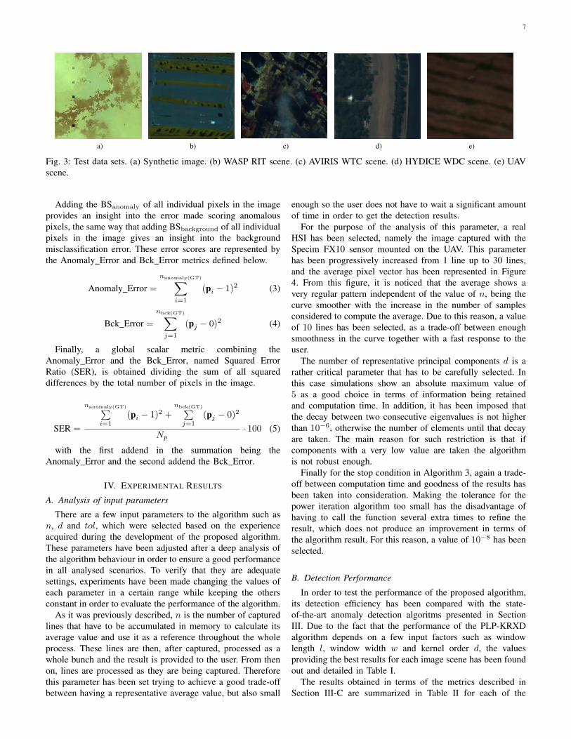
method. The simulated data have a size of 150x150 pixelsand 429 spectral bands. It was generated using a spectrallibrary collected from the United States Geological Survey(USGS) [27]. Background was simulated using four differentspectral signatures whose abundances were generated using aGaussian spherical distribution [28]. Twenty panels of differentsizes arranged in a 5x4 matrix were introduced as anomalies.There are five 4x4 pure-pixel panels lined up in five rows inthe first column, five 2x2 mixed-pixel panels in the secondcolumn, five subpixel panels combined with the backgroundin a proportion of 50% in the third column and five subpixelpanels blended with the background at 75%. Therefore, thesimulated image has 110 anomaly pixels, a 0.49% of theimage, as it is illustrated in Figure 3a. This data set is verychallenging for AD because of the high spectral similaritiesbetween some anomalous and background signatures.

In order to test the proposed algorithm in a more realisticscenario, four real hyperspectral data sets have been also used:three well known data sets available in the literature, anda data set captured by an UAV available at our lab. Thefirst real data set was taken over the Rochester Institute ofTechnology (RIT) by the Wildfire Airborne Sensor Program(WASP) Imaging System [29]. The system covers the visible,short, mid and long-wave infrared regions of the spectrum.The sensor was comprised by a high-resolution colour cameracovering the visible spectrum, a short infrared imager covering0.9 - 1.5 µm, mid infrared imager covering 3.0 - 5.0 µm anda long infrared imager covering 8.0 - 9.2 µm. A portion of theoverall image taken over a parking lot with a size of 180 x180 pixels and 120 bands has been used in this study, as canbe seen in Figure 3b where anomalies are fabric targets whichconsist of 72 pixels and account for 0.22% of the image. Thesecond real data set was collected by the NASA Jet PropulsionLaboratory's Airborne Visible Infra-Red Imaging Spectrometer(AVIRIS) over the World Trade Centre (WTC) area in NewYork City on September 16, 2001 [30]. The original dataset has a size of 614 x 512 pixels and 224 spectral bandsfrom 0.4 to 2.5 µm although a smaller region with size of200 x 200 pixels was selected as data set. Anomalies arethermal hot spots which consist of 83 pixels and account for0.21% of the image scene. Figure 3c shows a representationof this image. The third real data set is a portion of 67 × 80pixels cropped from the well−known Washington DC Mallhyperspectral data set, obtained through Purdue University’sMultiSpec freeware project. This data set was acquired by theairborne mounted Hyperspectral Digital Imagery CollectionExperiment (HYDICE) which measures pixel response in the0.4 to 2.4 µm region of the visible and infrared spectrum.Bands in the 0.9 and 1.4 µm region where the atmosphere isopaque have been omitted from the data set, leaving 191 bands.Figure 3d shows a RGB representation of the area chosen forthis analysis, which mainly consists of trees and a river andwhere the anomalous pixels belong to a building placed amongthe trees. The number of anomalous pixels is 15, 0.28 % ofthe image scene.

Finally, the last real HSI was captured by one of ourhyperspectral sensors mounted on an UAV. In particular, thesensor is the Specim hyperspectral FX10 which operates in

the visible and near infrared range (VNIR), i.e. between 0.4-1.0 µm. It is a push-broom camera which provides 1024 spatialpixels and 224 spectral bands [22]. However, due to the low-signal-to-noise ratio (SNR) of the first and last spectral bands,they were removed (1-10, 191-224), so that, 180 bands havebeen retained. The original image scene covers an area of1024x4967 pixels but a much shorter scene has been croppedcontaining the anomalies of the scene. Hence, the final sizeof the image utilized in this work is 250x250 pixels as shownin Figure 3e. Finally, it should be mentioned that the anomalytarget is a human being and that, in the whole scene, anomaliesconsist of 121 pixels, 0.19% of the total image while thebackground represented in the scene consists of a few rows ofwine crop and the soil in between.

B. Reference Algorithms

The LbL-AD algorithm has been compared against themost relevant algorithms of the state-of-the-art in the fieldof hyper-spectral AD, both computing the image as a wholeand in a line-by-line fashion as the LbL-AD algorithm does.The intention is to test the quality of the detection resultsand the separability between anomalies and background, aswell as the complexity and required computational effort.The selected algorithms are the Reed-Xiaoli after orthogonalsubspace projection (OSPRX), which computes the anomaliesonce the entire image is captured, and the progressive lineprocessing of kernel Reed-Xiaoli anomaly detection algorithmfor hyperspectral imagery PLP-KRXD [31], which follows aline-by-line fashion.

C. Assessment Metrics

Receiver Operating Characteristic (ROC) curves and thearea under these curves (AUC) have been widely used in theliterature to evaluate different anomaly detection algorithms.ROC curves are two dimensional graphical plots which illus-trate the relation between true positive rates (TPR) and falsepositive rates (FPR) obtained for various threshold settings.To compare the performance of several AD algorithms, AUCis used as a scalar measure, so that, a representation withthe biggest AUC outperforms the others. However, this metricdoes not always reflect how well the algorithm separates theanomalies from the background. For this reason, two extraquality metrics will be employed in this work: Brier Score(BS) and Squared Error Ratio (SER)[32].

BS measures the accuracy of probability predictions interms of marking anomalies and background pixels with thehighest and the lowest scores, respectively. If anomaly pixelsare represented as ones and background pixels as zeros in theground-truth, then, the BS for each type of pixel is calculatedas:

BSanomaly = (pi − 1)2; (1)

BSbackground = (pi − 0)2; (2)

being pi, the output of the algorithm, spanned in the range[0− 1].

7

a) b) c) d) e)

Fig. 3: Test data sets. (a) Synthetic image. (b) WASP RIT scene. (c) AVIRIS WTC scene. (d) HYDICE WDC scene. (e) UAVscene.

Adding the BSanomaly of all individual pixels in the imageprovides an insight into the error made scoring anomalouspixels, the same way that adding BSbackground of all individualpixels in the image gives an insight into the backgroundmisclassification error. These error scores are represented bythe Anomaly_Error and Bck_Error metrics defined below.

Anomaly_Error =

nanomaly(GT)∑i=1

(pi − 1)2 (3)

Bck_Error =

nbck(GT)∑j=1

(pj − 0)2 (4)

Finally, a global scalar metric combining theAnomaly_Error and the Bck_Error, named Squared ErrorRatio (SER), is obtained dividing the sum of all squareddifferences by the total number of pixels in the image.

SER =

nanomaly(GT)∑i=1

(pi − 1)2 +nbck(GT)∑j=1

(pj − 0)2

Np· 100 (5)

with the first addend in the summation being theAnomaly_Error and the second addend the Bck_Error.

IV. EXPERIMENTAL RESULTS

A. Analysis of input parameters

There are a few input parameters to the algorithm such asn, d and tol, which were selected based on the experienceacquired during the development of the proposed algorithm.These parameters have been adjusted after a deep analysis ofthe algorithm behaviour in order to ensure a good performancein all analysed scenarios. To verify that they are adequatesettings, experiments have been made changing the values ofeach parameter in a certain range while keeping the othersconstant in order to evaluate the performance of the algorithm.

As it was previously described, n is the number of capturedlines that have to be accumulated in memory to calculate itsaverage value and use it as a reference throughout the wholeprocess. These lines are then, after captured, processed as awhole bunch and the result is provided to the user. From thenon, lines are processed as they are being captured. Thereforethis parameter has been set trying to achieve a good trade-offbetween having a representative average value, but also small

enough so the user does not have to wait a significant amountof time in order to get the detection results.

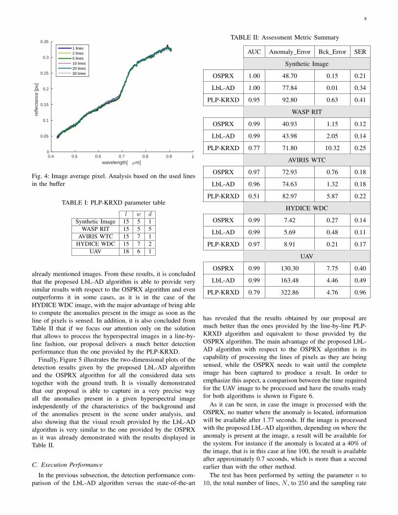
For the purpose of the analysis of this parameter, a realHSI has been selected, namely the image captured with theSpecim FX10 sensor mounted on the UAV. This parameterhas been progressively increased from 1 line up to 30 lines,and the average pixel vector has been represented in Figure4. From this figure, it is noticed that the average shows avery regular pattern independent of the value of n, being thecurve smoother with the increase in the number of samplesconsidered to compute the average. Due to this reason, a valueof 10 lines has been selected, as a trade-off between enoughsmoothness in the curve together with a fast response to theuser.

The number of representative principal components d is arather critical parameter that has to be carefully selected. Inthis case simulations show an absolute maximum value of5 as a good choice in terms of information being retainedand computation time. In addition, it has been imposed thatthe decay between two consecutive eigenvalues is not higherthan 10−6, otherwise the number of elements until that decayare taken. The main reason for such restriction is that ifcomponents with a very low value are taken the algorithmis not robust enough.

Finally for the stop condition in Algorithm 3, again a trade-off between computation time and goodness of the results hasbeen taken into consideration. Making the tolerance for thepower iteration algorithm too small has the disadvantage ofhaving to call the function several extra times to refine theresult, which does not produce an improvement in terms ofthe algorithm result. For this reason, a value of 10−8 has beenselected.

B. Detection Performance

In order to test the performance of the proposed algorithm,its detection efficiency has been compared with the state-of-the-art anomaly detection algoritms presented in SectionIII. Due to the fact that the performance of the PLP-KRXDalgorithm depends on a few input factors such as windowlength l, window width w and kernel order d, the valuesproviding the best results for each image scene has been foundout and detailed in Table I.

The results obtained in terms of the metrics described inSection III-C are summarized in Table II for each of the

8

wavelength[ 7m]0.4 0.5 0.6 0.7 0.8 0.9 1

refle

ctan

ce [p

u]

0

0.05

0.1

0.15

0.2

0.25

0.3

0.35

1 lines2 lines5 lines10 lines20 lines30 lines

Fig. 4: Image average pixel. Analysis based on the used linesin the buffer

TABLE I: PLP-KRXD parameter table

l w dSynthetic Image 15 5 1

WASP RIT 15 5 5AVIRIS WTC 15 7 1

HYDICE WDC 15 7 2UAV 18 6 1

already mentioned images. From these results, it is concludedthat the proposed LbL-AD algorithm is able to provide verysimilar results with respect to the OSPRX algorithm and evenoutperforms it in some cases, as it is in the case of theHYDICE WDC image, with the major advantage of being ableto compute the anomalies present in the image as soon as theline of pixels is sensed. In addition, it is also concluded fromTable II that if we focus our attention only on the solutionthat allows to process the hyperspectral images in a line-by-line fashion, our proposal delivers a much better detectionperformance than the one provided by the PLP-KRXD.

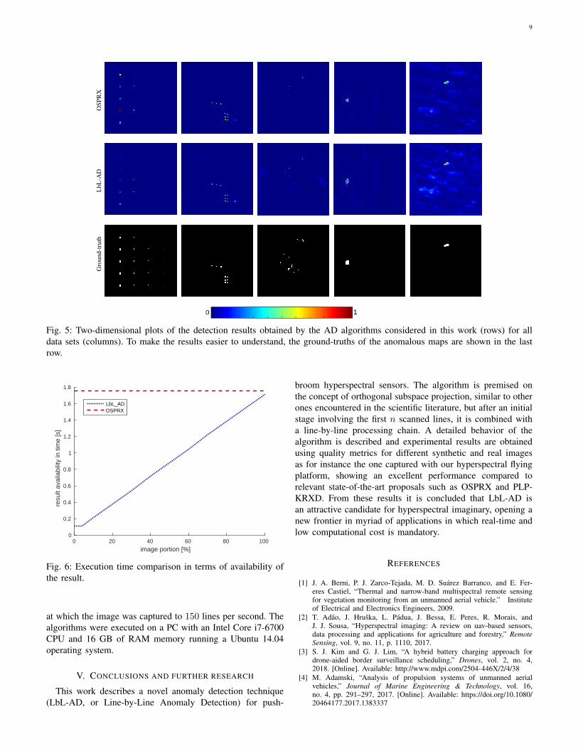
Finally, Figure 5 illustrates the two-dimensional plots of thedetection results given by the proposed LbL-AD algorithmand the OSPRX algorithm for all the considered data setstogether with the ground truth. It is visually demonstratedthat our proposal is able to capture in a very precise wayall the anomalies present in a given hyperspectral imageindependently of the characteristics of the background andof the anomalies present in the scene under analysis, andalso showing that the visual result provided by the LbL-ADalgorithm is very similar to the one provided by the OSPRXas it was already demonstrated with the results displayed inTable II.

C. Execution Performance

In the previous subsection, the detection performance com-parison of the LbL-AD algorithm versus the state-of-the-art

TABLE II: Assessment Metric Summary

AUC Anomaly_Error Bck_Error SER

Synthetic Image

OSPRX 1.00 48.70 0.15 0.21

LbL-AD 1.00 77.84 0.01 0.34

PLP-KRXD 0.95 92.80 0.63 0.41

WASP RIT

OSPRX 0.99 40.93 1.15 0.12

LbL-AD 0.99 43.98 2.05 0.14

PLP-KRXD 0.77 71.80 10.32 0.25

AVIRIS WTC

OSPRX 0.97 72.93 0.76 0.18

LbL-AD 0.96 74.63 1.32 0.18

PLP-KRXD 0.51 82.97 5.87 0.22

HYDICE WDC

OSPRX 0.99 7.42 0.27 0.14

LbL-AD 0.99 5.69 0.48 0.11

PLP-KRXD 0.97 8.91 0.21 0.17

UAV

OSPRX 0.99 130.30 7.75 0.40

LbL-AD 0.99 163.48 4.46 0.49

PLP-KRXD 0.79 322.86 4.76 0.96

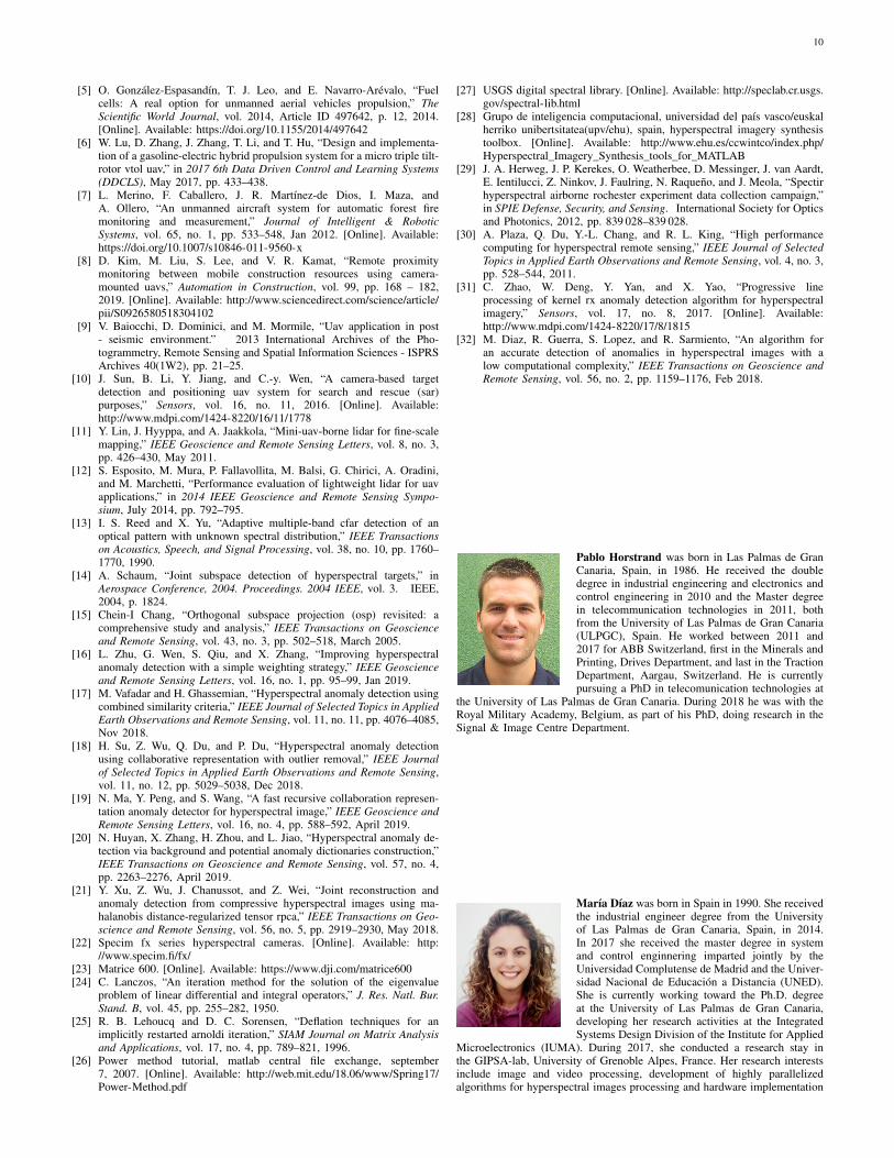
has revealed that the results obtained by our proposal aremuch better than the ones provided by the line-by-line PLP-KRXD algorithm and equivalent to those provided by theOSPRX algorithm. The main advantage of the proposed LbL-AD algorithm with respect to the OSPRX algorithm is itscapability of processing the lines of pixels as they are beingsensed, while the OSPRX needs to wait until the completeimage has been captured to produce a result. In order toemphasize this aspect, a comparison between the time requiredfor the UAV image to be processed and have the results readyfor both algorithms is shown in Figure 6.

As it can be seen, in case the image is processed with theOSPRX, no matter where the anomaly is located, informationwill be available after 1.77 seconds. If the image is processedwith the proposed LbL-AD algorithm, depending on where theanomaly is present at the image, a result will be available forthe system. For instance if the anomaly is located at a 40% ofthe image, that is in this case at line 100, the result is availableafter approximately 0.7 seconds, which is more than a secondearlier than with the other method.

The test has been performed by setting the parameter n to10, the total number of lines, N , to 250 and the sampling rate

9

OSP

RX

LbL

-AD

Gro

und-

trut

h

Fig. 5: Two-dimensional plots of the detection results obtained by the AD algorithms considered in this work (rows) for alldata sets (columns). To make the results easier to understand, the ground-truths of the anomalous maps are shown in the lastrow.

image portion [%]0 20 40 60 80 100

resu

lt av

aila

bilit

y in

tim

e [s

]

0

0.2

0.4

0.6

0.8

1

1.2

1.4

1.6

1.8

LbL_ADOSPRX

Fig. 6: Execution time comparison in terms of availability ofthe result.

at which the image was captured to 150 lines per second. Thealgorithms were executed on a PC with an Intel Core i7-6700CPU and 16 GB of RAM memory running a Ubuntu 14.04operating system.

V. CONCLUSIONS AND FURTHER RESEARCH

This work describes a novel anomaly detection technique(LbL-AD, or Line-by-Line Anomaly Detection) for push-

broom hyperspectral sensors. The algorithm is premised onthe concept of orthogonal subspace projection, similar to otherones encountered in the scientific literature, but after an initialstage involving the first n scanned lines, it is combined witha line-by-line processing chain. A detailed behavior of thealgorithm is described and experimental results are obtainedusing quality metrics for different synthetic and real imagesas for instance the one captured with our hyperspectral flyingplatform, showing an excellent performance compared torelevant state-of-the-art proposals such as OSPRX and PLP-KRXD. From these results it is concluded that LbL-AD isan attractive candidate for hyperspectral imaginary, opening anew frontier in myriad of applications in which real-time andlow computational cost is mandatory.

REFERENCES

[1] J. A. Berni, P. J. Zarco-Tejada, M. D. Suárez Barranco, and E. Fer-eres Castiel, “Thermal and narrow-band multispectral remote sensingfor vegetation monitoring from an unmanned aerial vehicle.” Instituteof Electrical and Electronics Engineers, 2009.

[2] T. Adão, J. Hruška, L. Pádua, J. Bessa, E. Peres, R. Morais, andJ. J. Sousa, “Hyperspectral imaging: A review on uav-based sensors,data processing and applications for agriculture and forestry,” RemoteSensing, vol. 9, no. 11, p. 1110, 2017.

[3] S. J. Kim and G. J. Lim, “A hybrid battery charging approach fordrone-aided border surveillance scheduling,” Drones, vol. 2, no. 4,2018. [Online]. Available: http://www.mdpi.com/2504-446X/2/4/38

[4] M. Adamski, “Analysis of propulsion systems of unmanned aerialvehicles,” Journal of Marine Engineering & Technology, vol. 16,no. 4, pp. 291–297, 2017. [Online]. Available: https://doi.org/10.1080/20464177.2017.1383337

10

[5] O. González-Espasandín, T. J. Leo, and E. Navarro-Arévalo, “Fuelcells: A real option for unmanned aerial vehicles propulsion,” TheScientific World Journal, vol. 2014, Article ID 497642, p. 12, 2014.[Online]. Available: https://doi.org/10.1155/2014/497642

[6] W. Lu, D. Zhang, J. Zhang, T. Li, and T. Hu, “Design and implementa-tion of a gasoline-electric hybrid propulsion system for a micro triple tilt-rotor vtol uav,” in 2017 6th Data Driven Control and Learning Systems(DDCLS), May 2017, pp. 433–438.

[7] L. Merino, F. Caballero, J. R. Martínez-de Dios, I. Maza, andA. Ollero, “An unmanned aircraft system for automatic forest firemonitoring and measurement,” Journal of Intelligent & RoboticSystems, vol. 65, no. 1, pp. 533–548, Jan 2012. [Online]. Available:https://doi.org/10.1007/s10846-011-9560-x

[8] D. Kim, M. Liu, S. Lee, and V. R. Kamat, “Remote proximitymonitoring between mobile construction resources using camera-mounted uavs,” Automation in Construction, vol. 99, pp. 168 – 182,2019. [Online]. Available: http://www.sciencedirect.com/science/article/pii/S0926580518304102

[9] V. Baiocchi, D. Dominici, and M. Mormile, “Uav application in post- seismic environment.” 2013 International Archives of the Pho-togrammetry, Remote Sensing and Spatial Information Sciences - ISPRSArchives 40(1W2), pp. 21–25.

[10] J. Sun, B. Li, Y. Jiang, and C.-y. Wen, “A camera-based targetdetection and positioning uav system for search and rescue (sar)purposes,” Sensors, vol. 16, no. 11, 2016. [Online]. Available:http://www.mdpi.com/1424-8220/16/11/1778

[11] Y. Lin, J. Hyyppa, and A. Jaakkola, “Mini-uav-borne lidar for fine-scalemapping,” IEEE Geoscience and Remote Sensing Letters, vol. 8, no. 3,pp. 426–430, May 2011.

[12] S. Esposito, M. Mura, P. Fallavollita, M. Balsi, G. Chirici, A. Oradini,and M. Marchetti, “Performance evaluation of lightweight lidar for uavapplications,” in 2014 IEEE Geoscience and Remote Sensing Sympo-sium, July 2014, pp. 792–795.

[13] I. S. Reed and X. Yu, “Adaptive multiple-band cfar detection of anoptical pattern with unknown spectral distribution,” IEEE Transactionson Acoustics, Speech, and Signal Processing, vol. 38, no. 10, pp. 1760–1770, 1990.

[14] A. Schaum, “Joint subspace detection of hyperspectral targets,” inAerospace Conference, 2004. Proceedings. 2004 IEEE, vol. 3. IEEE,2004, p. 1824.

[15] Chein-I Chang, “Orthogonal subspace projection (osp) revisited: acomprehensive study and analysis,” IEEE Transactions on Geoscienceand Remote Sensing, vol. 43, no. 3, pp. 502–518, March 2005.

[16] L. Zhu, G. Wen, S. Qiu, and X. Zhang, “Improving hyperspectralanomaly detection with a simple weighting strategy,” IEEE Geoscienceand Remote Sensing Letters, vol. 16, no. 1, pp. 95–99, Jan 2019.

[17] M. Vafadar and H. Ghassemian, “Hyperspectral anomaly detection usingcombined similarity criteria,” IEEE Journal of Selected Topics in AppliedEarth Observations and Remote Sensing, vol. 11, no. 11, pp. 4076–4085,Nov 2018.

[18] H. Su, Z. Wu, Q. Du, and P. Du, “Hyperspectral anomaly detectionusing collaborative representation with outlier removal,” IEEE Journalof Selected Topics in Applied Earth Observations and Remote Sensing,vol. 11, no. 12, pp. 5029–5038, Dec 2018.

[19] N. Ma, Y. Peng, and S. Wang, “A fast recursive collaboration represen-tation anomaly detector for hyperspectral image,” IEEE Geoscience andRemote Sensing Letters, vol. 16, no. 4, pp. 588–592, April 2019.

[20] N. Huyan, X. Zhang, H. Zhou, and L. Jiao, “Hyperspectral anomaly de-tection via background and potential anomaly dictionaries construction,”IEEE Transactions on Geoscience and Remote Sensing, vol. 57, no. 4,pp. 2263–2276, April 2019.

[21] Y. Xu, Z. Wu, J. Chanussot, and Z. Wei, “Joint reconstruction andanomaly detection from compressive hyperspectral images using ma-halanobis distance-regularized tensor rpca,” IEEE Transactions on Geo-science and Remote Sensing, vol. 56, no. 5, pp. 2919–2930, May 2018.

[22] Specim fx series hyperspectral cameras. [Online]. Available: http://www.specim.fi/fx/

[23] Matrice 600. [Online]. Available: https://www.dji.com/matrice600[24] C. Lanczos, “An iteration method for the solution of the eigenvalue

problem of linear differential and integral operators,” J. Res. Natl. Bur.Stand. B, vol. 45, pp. 255–282, 1950.

[25] R. B. Lehoucq and D. C. Sorensen, “Deflation techniques for animplicitly restarted arnoldi iteration,” SIAM Journal on Matrix Analysisand Applications, vol. 17, no. 4, pp. 789–821, 1996.

[26] Power method tutorial, matlab central file exchange, september7, 2007. [Online]. Available: http://web.mit.edu/18.06/www/Spring17/Power-Method.pdf

[27] USGS digital spectral library. [Online]. Available: http://speclab.cr.usgs.gov/spectral-lib.html

[28] Grupo de inteligencia computacional, universidad del país vasco/euskalherriko unibertsitatea(upv/ehu), spain, hyperspectral imagery synthesistoolbox. [Online]. Available: http://www.ehu.es/ccwintco/index.php/Hyperspectral_Imagery_Synthesis_tools_for_MATLAB

[29] J. A. Herweg, J. P. Kerekes, O. Weatherbee, D. Messinger, J. van Aardt,E. Ientilucci, Z. Ninkov, J. Faulring, N. Raqueño, and J. Meola, “Spectirhyperspectral airborne rochester experiment data collection campaign,”in SPIE Defense, Security, and Sensing. International Society for Opticsand Photonics, 2012, pp. 839 028–839 028.

[30] A. Plaza, Q. Du, Y.-L. Chang, and R. L. King, “High performancecomputing for hyperspectral remote sensing,” IEEE Journal of SelectedTopics in Applied Earth Observations and Remote Sensing, vol. 4, no. 3,pp. 528–544, 2011.

[31] C. Zhao, W. Deng, Y. Yan, and X. Yao, “Progressive lineprocessing of kernel rx anomaly detection algorithm for hyperspectralimagery,” Sensors, vol. 17, no. 8, 2017. [Online]. Available:http://www.mdpi.com/1424-8220/17/8/1815

[32] M. Diaz, R. Guerra, S. Lopez, and R. Sarmiento, “An algorithm foran accurate detection of anomalies in hyperspectral images with alow computational complexity,” IEEE Transactions on Geoscience andRemote Sensing, vol. 56, no. 2, pp. 1159–1176, Feb 2018.

Pablo Horstrand was born in Las Palmas de GranCanaria, Spain, in 1986. He received the doubledegree in industrial engineering and electronics andcontrol engineering in 2010 and the Master degreein telecommunication technologies in 2011, bothfrom the University of Las Palmas de Gran Canaria(ULPGC), Spain. He worked between 2011 and2017 for ABB Switzerland, first in the Minerals andPrinting, Drives Department, and last in the TractionDepartment, Aargau, Switzerland. He is currentlypursuing a PhD in telecomunication technologies at

the University of Las Palmas de Gran Canaria. During 2018 he was with theRoyal Military Academy, Belgium, as part of his PhD, doing research in theSignal & Image Centre Department.

María Díaz was born in Spain in 1990. She receivedthe industrial engineer degree from the Universityof Las Palmas de Gran Canaria, Spain, in 2014.In 2017 she received the master degree in systemand control enginnering imparted jointly by theUniversidad Complutense de Madrid and the Univer-sidad Nacional de Educación a Distancia (UNED).She is currently working toward the Ph.D. degreeat the University of Las Palmas de Gran Canaria,developing her research activities at the IntegratedSystems Design Division of the Institute for Applied

Microelectronics (IUMA). During 2017, she conducted a research stay inthe GIPSA-lab, University of Grenoble Alpes, France. Her research interestsinclude image and video processing, development of highly parallelizedalgorithms for hyperspectral images processing and hardware implementation

11

Raúl Guerra was born in Las Palmas de GranCanaria, Spain, in 1988. He received the industrialengineer degree by the University of Las Palmasde Gran Canaria in 2012. In 2013 he received themaster degree in telecommunications technologiesimparted by the Institute of Applied Microelectron-ics, IUMA. He was funded by this institute to dohis PhD research in the Integrated System DesignDivision, receiving his PhD in TelecommunicationsTechnologies by the University of Las Palmas deGran Canarias in 2017. During 2016 he worked as

a researcher in the Configurable Computing Lab in Virginia Tech University.His current research interests include the parallelization of algorithms for mul-tispectral and hyperspectral images processing and hardware implementation.

Sebastián López (M’08 - SM’15) was born in LasPalmas de Gran Canaria, Spain, in 1978. He receivedthe electronic engineering degree from the Univer-sity of La Laguna, San Cristobal de La Laguna,Spain, in 2001, and the Ph.D. degree in electronicengineering from the University of Las Palmas deGran Canaria, Las Palmas de Gran Canaria, in2006. He is currently an Associate Professor withthe University of Las Palmas de Gran Canaria,where he is involved in research activities with theIntegrated Systems Design Division, Institute for

Applied Microelectronics. He has co-authored more than 120 papers ininternational journals and conferences. His research interests include real-time hyperspectral imaging, reconfigurable architectures, high-performancecomputing systems, and image and video processing and compression. Dr.LÃspez was a recipient of regional and national awards during his electronicengineering degree. He is an Associate Editor of the IEEE Journal of SelectedTopics in Applied Earth Observations and Remote Sensing, MDPI RemoteSensing, and the Mathematical Problems in Engineering Journal. He was anAssociate Editor of the IEEE Transactions on Consumer Electronics from2008 to 2013. He also serves as an active reviewer for different JCR journalsand as program committee member of a variety of reputed internationalconferences. Furthermore, he acted as one of the program chairs of theIEEE Workshop on Hyperspectral Image and Signal Processing: Evolution inRemote Sensing (WHISPERS) in its 2014 edition and of the SPIE Conferenceof High Performance Computing in Remote Sensing from 2015 to 2018.Moreover, he has been the Guest Editor of different special issues in JCRjournals related with his research interests.

José F. López received the M.S. degree in physics(specializing in electronics) from the University ofSeville and the Ph.D. degree from the Universityof Las Palmas de Gran Canaria (ULPGC), Spain,being awarded by this University for his researchin the field of High Speed Integrated Systems. Hehas conducted his investigations at the Institute forApplied Microelectronics (IUMA), where he acts asDeputy Director since 2009. He currently lecturesat the School of Telecommunication & ElectronicsEngineering and at the MSc. Program of IUMA, in

the ULPGC. He was with Thomson Composants Microondes, Orsay, France,in 1992. In 1995 he was with the Center for Broadband Telecommunicationsat the Technical University of Denmark (DTU), Lyngby, Denmark, and in1996, 1997, 1999, and 2000, he was visiting researcher at Edith CowanUniversity (ECU), Perth, Western Australia. Presently his main areas ofinterest are in the field of image processing, UAVs, hyperspectral technologyand their applications. Dr. López has been actively enrolled in more than 40research projects funded by the European Community, Spanish Governmentand international private industries located in Europe, USA and Australia.He has written around 140 papers in national and international journals andconferences.

View publication statsView publication stats