A new Convection Parameterization:A new Convection Parameterization:

Some Achievements and Some ChallengesSome Achievements and Some Challenges

Hans-F Graf, Cambridge

Till M Wagner, Oxford (was Cambridge )

IPAM, UCLA, May 2010

Some motivation:Some motivation:

- Clouds are beautiful

- Clouds drive general circulation

Convective clouds Radiation

Layered clouds Turbulence

- Clouds are un-resolved

State of the art:State of the art:

Separation into stratiform and convective clouds, detraining water from convective clouds is source for stratiform clouds => radiative effects

If convective clouds change so do stratiform.

water

Latent heat

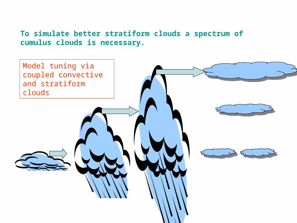
To simulate better stratiform clouds a spectrum of cumulus clouds is necessary.

Model tuning via coupled convective and stratiform clouds

Disparity of Scales• Deep convective clouds

– larger vertical than horizontal extent– reaching depth of a few to several kilometres

• Boundary layer clouds– on top of turbulent boundary layer– 100m to one kilometre thick

• Explicit representation in numerical model requires horizontal to vertical aspect ratio < 1:– dx < 5km for deep convective clouds– dx < 1km for boundary layer clouds

• Current horizontal spatial resolution too coarse

– in climate models: dx = 100-200 km– convection unresolved– paramaterization needed to include effect

Vertical scales:Vertical scales:Since in-cloud vertical temperature gradient is ~6K/1km a vertical model resolution of 1 km in the middle troposphere is inadequate to find the freezing level.

However, freezing is critical for cloud microphysics, efficiency of rain formation and, ultimately, latent heat release.

Also aerosol- cloud microphysics interaction effects may critically depend on whether mixed phase is reached and this may affect the maximum cloud height, especially if weak free tropospheric inversion layers are present.

Hence, deep convection parameterization has to be done on higher vertical resolution of the order of 100 m. (Graf 2004)

Convection Parameterizations

• Adjustment schemes (Manabe, 1965): – Only temperature, moisture adjustment– No transport– No microphysics

• Moisture budget schemes (Kuo, 1974): – Redistribution of temperature, moisture– Coupled to moisture convergence

• Spectral mass flux scheme (Arakawa & Schubert, 1974)– Too difficult

• Bulk mass flux schemes (Tiedtke, 1989; Gregory & Rowntree, 1990): – Temperature, moisture, momentum, tracer transport– Basic microphysics

Quasi-equilibrium closure!

Arakawa-Schubert parameterisationquasi-equilibrium closure

• Solve

for to determine the cloud mass flux

• Characteristics– Mass flux must be positive semidefinite ( ) – Positive semidefiniteness of solution not guaranteed

usually no exact solution possible approximate/optimal solution (Lord, 1982; Hack et al, 1984)

Kij = effect of cloud j on cloud i, Fi = environmental forcing for cloud i

MBj = mass flux at base of cloud j

• Goals

– Better representation of dynamics and microphysics

• mixed phase microphysics

• droplet nucleation & cloud ice initiation

– Additional in-cloud variables besides massflux

• vertical velocity spectrum

• super-saturation & nucleation rate

• Concept:

single cloud model + cloud spectrum calculation

Convective Cloud Field Model

Nober and Graf 2005

Model Concept –single cloud model

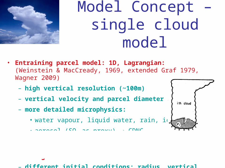
• Entraining parcel model: 1D, Lagrangian:(Weinstein & MacCready, 1969, extended Graf 1979, Wagner 2009)

– high vertical resolution (~100m)

– vertical velocity and parcel diameter

– more detailed microphysics:

• water vapour, liquid water, rain, ice, snow

• aerosol (SO4 as proxy) CDNC

• Calculates cloud types that can potentially exist within grid cell

– different initial conditions: radius, vertical velocity

Model Concept - cloud spectrum calculation

• Multivariate Lotka-Volterra (LV) system of ODEs

– describes competitive system of N species

• Dynamical closure of Arakawa-Schubert type

– clouds forced by environment (CAPE)

– clouds mutually interactvia influence of the environment

– dynamical evolution of cloud spectrumwithin large scale time step

(Arakawa and Schubert, 1974)

Convective Cloud Field Model- dynamical cloud balance

• Multivariate Lotka-Volterra (LV) system of ODEs

• Describes competitive system of N species

• Carrying capacity of species i :

– Equilibrium amount of species i in absence of other species

– Used as solution of the relaxed Arakawa-Schubert scheme (just one cloud at a time, Moorthi & Suarez, 1992)

K = cloud-cloud interaction

F = environment impact on cloud

A = cloud work function (conversion of potential to kinetic energy)

ni = number of species i

Comparing AS against CCFM:

Convective cloud field closure formulation can be regarded as a generalisation of the quasi-equilibrium equation of Arakawa and Schubert (1974) dropping two assumptions:

1) kinetic energy equilibrium dK/dt = 0 is not assumed

2) stationarity, i.e. dx/dt = 0 or equivalently dM/dt = 0 is not assumed

Further, an explicit cloud model is used and this allows to also include explicit vertical velocities and a much better possibility to include more complex cloud microphysics (e.g. activation of CCN!).

For those wishing the details:

The original model was completely rewritten, tested and a solid mathematical derivation and description is provided here:

CCFM is now included into Global Climate Model (ECHAM5-HAM, also in single column mode!) and Limited Area Model (REMO and REMOTE)

In single column mode both reanalysis and radio sonde data can be used to facilitate comparison against observations.

For initializing the cloud spectrum a maximum cloud base radius is determined from the height of PBL. Then a number (usually 15-20) of smaller initial cloud radii is set down to a minimum of 100m.

First guess of cloud spectrum results from carrying capacity.

Vertical velocity at cloud base is dependent on TKE.

There are only few useful data sets to compare a model with reality. One of those is from ARM stations.

CCFM in single column mode clearly much improves the sequence of precipitation events and their variable intensity both, over land and over tropical ocean.

One of the really nice features of CCFM is that it allows to identify rainfall intensity spectra for each time step and for each grid cell.

The daily cycle of precipitation very closely follows observations.

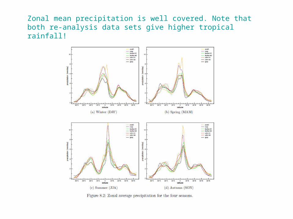
Zonal mean precipitation is well covered. Note that both re-analysis data sets give higher tropical rainfall!

Annual mean precipitation

Only sparse observations!

ECHAM5-CCFM is in ballpark of re-analysis and the highly tuned ECHAM5-Tiedtke.

CCFM reduces bias in tropical West Pacific but introduces problems in tropical Indian Ocean.

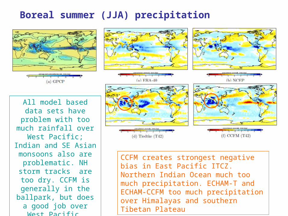
Boreal summer (JJA) precipitation

All model based data sets have problem with too

much rainfall over West Pacific; Indian and SE

Asian monsoons also are problematic. NH storm

tracks are too dry. CCFM is generally in the ballpark, but does a good job over

West Pacific.

CCFM creates strongest negative bias in East Pacific ITCZ. Northern Indian Ocean much too much precipitation. ECHAM-T and ECHAM-CCFM too much precipitation over Himalayas and southern Tibetan Plateau

Anomalous cyclonic circulation, forced by convective heating?

Anomalously strong low and convergence over Tibetan Plateau forced by radiative heating?

Wind vectors and geopotential difference from zonal mean during the Indian summer monsoon season.

The Tibet problem

What is the effect of the daily cycle in cloud cover on the radiative budget?

Diffuse radiation is minimal

Solar constant

PBL clouds like Cu hum are not present in the models, hence solar radiation directly heats the ground, creating a strong heat low and this affects large scale circulation and moisture transport.

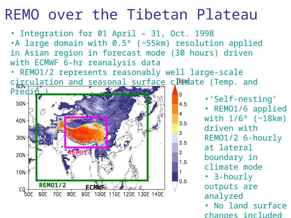
REMO over the Tibetan Plateau• Integration for 01 April – 31, Oct. 1998 •A large domain with 0.5º (~55km) resolution applied in Asian region in forecast mode (30 hours) driven with ECMWF 6-hr reanalysis data• REMO1/2 represents reasonably well large-scale circulation and seasonal surface climate (Temp. and Precip.)

REMO1/2

REMO1/6

ECMWF

•‘Self-nesting’• REMO1/6 applied with 1/6º (~18km) driven with REMO1/2 6-hourly at lateral boundary in climate mode• 3-hourly outputs are analyzed• No land surface changes included

REMO 1/2o REMO 1/6o

Direct comparison of rainfall simulated by REMO at different resolution, driven 6-hourly by ECMWF re-analysis for two well maintained stations (GAME-Tibet). Cui et al. 2007

While REMO 1/2 fails to simulate correct precipitation amount, REMO 1/6 does well. The coarse model produces less latent heat and surface cooling.

The Tibet problem …

Is very much a problem of resolution.

The Indian summer monsoon problem

What is the contribution of aerosol-microphysics interaction to the solution?

The Indian summer monsoon bias of ECHAM is enhanced by CCFM

Adding aerosols over land slightly improves the situation…

Echam5-Tiedtke Echam5-CCFM

SEA summer monsoon:

Too much rain over Arabian Sea and Bay of Bengal, too much right over Himalayas and ECHAM-T too much over warm pool.

Increasing the number of aerosol particles simply by factor of 10 over land and sea has strong impact on BoB precipitation and South China Sea. There precipitation bias decreases. Arabian Sea bias slightly enhances. ECHAM5-CCFM 10xCCN

Using CCFM in the ECHAM-HAM (including prognostic aerosol) environment will have strong impact on model performance.

Strong winds over Arabian Sea lead to enhanced water vapour flux?

Enhanced trough over Bay of Bengal enhancing convection?

CCFM already now improves geopotential height distribution, problems over Tibet remain as do the strong winds over the warm waters of the Indian Ocean.

The Indian summer monsoon problem

Is more complex since it involves a number of processes not covered completely by convection parameterization.

Conclusions

CCFM is a new parameterization of convective clouds that has a number of benefits. It is, without any tuning, able to reproduce and to also at some places improve simulated convective activity.

If run in SCM (without large scale the biases of the host model) CCFM strongly improves precipitation and related parameters.

This gives space for further improvements, especially since processes like microphysics in convective clouds, impact of aerosols of different nature can relatively easily be included.

CCFM provides more information (e.g. on convective transport, spectrum of precipitation intensity etc.) than other parameterizations.

Challenges remain with respect to organized convection, entrainment and detrainment profiles, close link to stratiform clouds, and others.