A monotone nonlinear ﬁnite volume method for advection...

Russ. J. Numer. Anal. Math. Modelling, Vol. 25, No. 4, pp. 335–358 (2010)

DOI 10.1515/ RJNAMM.2010.022

c© de Gruyter 2010

A monotone nonlinear finite volume method

for advection–diffusion equationson unstructured polyhedral meshes in 3D

K. NIKITIN∗ and Yu. VASSILEVSKI∗

Abstract — We present a new monotone finite volume method for the advection–diffusion equationwith a full anisotropic discontinuous diffusion tensor and a discontinuous advection field on 3D con-formal polyhedral meshes. The proposed method is based on a nonlinear flux approximation both fordiffusive and advective fluxes and guarantees solution non-negativity. The approximation of the dif-fusive flux uses the nonlinear two-point stencil described in [9]. Approximation of the advective fluxis based on the second-order upwind method with a specially designed minimal nonlinear correction[26]. The second-order convergence rate and monotonicity are verified with numerical experiments.

The discrete maximum principle (DMP) and local mass conservation are importantproperties of a numerical scheme for the approximate solution of the steady stateadvection–diffusion equation. An accurate discretization method satisfying DMP ishard to develop. We address the monotonicity condition as the simplified versionof the DMP, which guarantees only solution non-negativity. A number of physicalquantities (concentration, temperature, etc.) are non-negative by their nature andtheir approximations should be non-negative as well. We present a nonlinear finitevolume (FV) method on conformal polyhedral meshes that satisfies the monotonic-ity condition for a wide range of problem coefficients. We admit a jumping diffusioncoefficient represented by full anisotropic tensors, a jumping advection coefficient,which may be produced by the Darcy equation in multimaterial media, and bothdiffusion-dominated and advection-dominated regimes. The presented method isthe extension of numerical schemes [9, 26] developed for the 3D diffusion equation[9] and the 2D advection–diffusion equation with continuous coefficients [26].

The major difficulty encountered in the design of a monotone numerical schemeis suppressing unwanted spurious (non-physical) oscillations in the numerical solu-tion. These oscillations may appear in advection-dominated problems due to in-ternal shocks and boundary layers, and in diffusion-dominated problems in highlyanisotropic media due to inappropriate approximations of the diffusive flux.

In the finite element (FE) context, efficient damping of spurious oscillationsin advection-dominated regimes has been developed within the streamline upwind

∗Institute of Numerical Mathematics, Russian Academy of Sciences, Moscow 119333, Russia

This work has been supported in part by RFBR grants 08-01-00159, 09-01-00115, Federal Pro-gram ‘Scientific and Educational Stuff of Innovative Russia’, and grant from Upstream Research Cen-ter, ExxonMobil corp.

336 K. Nikitin and Yu. Vassilevski

Petrov–Galerkin (SUPG) method [5]. However, spurious oscillations around sharplayers may still appear in the SUPG solution. Spurious oscillations at layers dimi-nishing (SOLD) methods [11] are generalizations of SUPG, which satisfy the DMPat least in some model cases. Spurious oscillations of FE solutions in diffusion-dominated regimes are caused by approximation difficulties in the case of generalmeshes and diffusion tensors. The theoretical analysis of DMP in the FE methods[8, 15, 32] imposes severe restrictions on the coefficients and the computationalmesh. An algebraic flux correction [16, 17] is the alternative approach to the designof monotone FE methods. We note, however, that many FE methods are formallynot locally conservative on the cells of the original computational mesh.

The finite volume (FV) methods, in contrast, guarantee the local mass conserva-tion by their construction. The development of new FV methods for the advection–diffusion equation has been a popular topic of research, (see [3, 4, 10, 20, 28, 36])for the steady equation and [35] for the unsteady equation and references therein).The advective fluxes can be approximated via the upwinding approach and con-trolled with different slope-limiting techniques [4, 7, 23] or the introduction ofartificial viscosity [2, 28]. Many advanced second-order accurate linear methodsfor the diffusion equation fail to satisfy the monotonicity condition [1, 24, 30].Nonlinear methods have seemed to be the feasible approach towards monotoneand second-order accurate discretization [4, 11]. Nonlinear methods have beendeveloped for the Poisson equation [6] and for the general diffusion equation[9, 14, 18, 21, 22, 24, 27, 29, 35, 37].

Our approximation of the advective flux is the 3D extension of the 2D nonli-near method proposed in [26]. The method follows the idea of the MUSCL method[34] and uses a piecewise linear discontinuous reconstruction of the FV solutionon polyhedral cells, whose slope is limited via a three-by-three matrix with nonlin-ear entries. More precisely, we minimize the deviation of the reconstructed linearfunction from the given values at selected points subject to some monotonicity con-straints, which form a convex set in the space of the function gradient components.The constraints are related to those considered in [12], but differ in the set of se-lected points and in the norm of deviation.

For the discretization of the diffusive flux we adopt the nonlinear two-pointflux approximation on polyhedral meshes proposed in [9]. The original idea wasproposed by Le Potier in [21] for the explicit scheme for the unsteady diffusionequation on triangular meshes. Further developments of the method [14, 24, 35, 37]extend it to a wider class of meshes and equations, but inherit the interpolation fromprimary unknowns defined at the mesh cells to secondary unknowns at the meshvertices. The use of interpolation affects the accuracy of the numerical scheme,as well as the properties of nonlinear solvers. An interpolation-free nonlinear FVmethod on 2D meshes with polygonal cells was developed in [25]. It was extendedto polyhedral meshes in [9] using physical interpolation for secondary unknowns atboundary faces and faces where the diffusion tensor jumps.

The proposed FV method is exact for linear solutions. Therefore, for problemswith smooth solutions, one can expect the second-order asymptotic convergence

A monotone nonlinear finite volume method 337

rate, which is confirmed in our numerical experiments. The monotone properties ofthe discrete solution are illustrated by the numerical experiments as well. The two-point stencil for flux approximation results in sparse matrices even on polyhedralmeshes. For cubic meshes and a diagonal diffusion tensor these matrices reduce tothe conventional 7-point discretization. Although the method is not interpolation-free, most of the interpolation operations are based on physical principles and thusdo not affect the numerical properties of the method.

The major computational overhead in nonlinear FV methods is related to twonested iterations in the solution of a nonlinear algebraic problem. The outer iterationis the Picard method, which guarantees the solution non-negativity on each iteration.The set of admissible gradients in linear reconstruction used in the discretization ofthe advective fluxes is chosen to guarantee the stability of Picard iterations. Theinner iteration is the Krylov subspace method for solving linearized problems.

The paper outline is as follows. In Section 1, we state the steady advection–diffusion problem. In Section 2, we describe the construction of discrete fluxeswhich form the basis of our method. In Section 3, we discuss the properties of theresulting algebraic system and present our algorithm for the generation and solu-tion of that system. In Section 4, we present the numerical properties of the schemeusing tetrahedral, hexahedral, and triangular prismatic meshes.

1. Steady-state advection–diffusion equation

Let Ω be a three-dimensional polyhedral domain with the boundary Γ = ΓN ∪ΓD where ΓD ∩ ΓN = ∅ and ΓD has a non-zero measure. We consider a modeladvection–diffusion problem for an unknown concentration c [see 19, 31]:

div (vc−K∇c) = g in Ω

c = gD on ΓD (1.1)

−(K∇c) ·n = gN on ΓN

where K(x) is a symmetric positive definite possibly anisotropic piecewise conti-nuous diffusion tensor, v(x) is a piecewise continuous velocity field, g ∈ L2(Ω) isa source term, n is the exterior normal vector, and gD, gN are given boundary data.It is known [19] that under the above assumptions and appropriate restrictions on

gD, gN , equation (1.1) has a unique weak solution c ∈W 10 (Ω). We denote by Γout

the outflow part of Γ where v · n > 0, and define Γin = Γ \Γout. We assume thatΓN ⊂ Γout.

The sufficient conditions for the non-negativity of the solution c(x) are g(x) >

0, gD > 0, and gN 6 0. We assume that these conditions hold. From a physicalviewpoint, the requirements g(x) > 0 and gN 6 0 mean that no mass can be takenout of the system.

The Dirichlet boundary condition on Γout and the discontinuity in boundary dataon Γin may result in parabolic boundary layers. Exponential boundary layers mayappear at the part of Γout where v ·n > 0. An ideal discretization scheme must add


a numerical diffusion, which is small enough to avoid excessive smearing of theboundary layers, but sufficient to damp non-physical oscillations.

2. Monotone nonlinear FV scheme on polyhedral meshes

In this section, we derive a FV scheme with a nonlinear two-point flux approxi-mation. Let q = −K∇c+ cv denote the total flux, which satisfies the mass balanceequation:

div q = g inΩ. (2.1)

Let T be a conformal polyhedral mesh composed of NT shape-regular cellswith planar faces. We assume that each cell is a star-shaped 3D domain with respectto its barycenter, and each face is a star-shaped 2D domain with respect to the face’sbarycenter. We assume that T is face-connected, i.e. it cannot be split into twomeshes having no common faces. We also assume that the tensor function K(x) andthe velocity field v(x) vary slightly inside each cell and div v ∈ L2(Ω), div v > 0for almost every x ∈ Ω; however K and v may jump across the mesh faces, as wellas may change the direction (the principal directions for K), although the normalcomponent of vmust be continuous on any mesh face. We denote by nT the exteriorunit normal vector to ∂T and by n f the normal vector to face f fixed once and forall. On a boundary face, the vector n f is exterior. We assume that |n f | = | f | where| f | denotes the area of face f .

Let NB be the number of boundary faces. By FI , FB we denote disjoint sets ofinterior and boundary faces. The subset FJ of FI includes the faces where K(x) orv(x) jump. The set FB is further split into subsets FD

B and FNB where the Dirichlet

and Neumann boundary conditions, respectively, are imposed. Alternatively, the setFB is split into subsets F out

B and F inB of faces belonging to Γout and Γin, respec-

tively. Finally, FT and ET denote the sets of the faces and edges of the polyhedronT respectively, whereas E f denotes the set of the edges of the face f .

Integrating equation (2.1) over a polyhedron T and using Green’s formula weget:

∑f∈∂T

χT, f q f ·n f =∫

Tf dx, q f =

1

| f |

∫

fqds (2.2)

where q f is the average flux density for the face f , and χT, f is either 1 or −1,depending on the mutual orientation of the normal vectors n f and nT .

For each cell T , we assign one degree of freedom, CT , for the concentrationc. Let C be the vector of all discrete concentrations. If two cells T+ and T− havea common face f and n f is exterior to T+, the two-point flux approximation is asfollows:

qhf ·n f = M+f CT+ −M−

f CT− (2.3)

where M+f and M−

f are some coefficients. In a linear FV method, these coefficients

are equal and fixed. In the nonlinear FV method, they may be different and dependon the concentrations in the adjacent cells. On a face f ∈ ΓD, the flux has a form


similar to (2.3) with an explicit value for one of the concentrations. For the Dirichletboundary value problem, ΓD = ∂Ω, substituting (2.3) into (2.2), we obtain a systemof NT equations with NT unknowns CT .

Therefore, the cornerstone of the cell–centered FV method is the definition ofdiscrete flux (2.3). Our method of the discrete flux definition generalizes the defini-tion of the diffusive flux [9] to the case of an advective–diffusive flux on the basisof the 2D method [26]. In order to present our method, we introduce the notationsborrowing them from [9].

For every cell T in T , we define the collocation point xT at the barycenter ofT . For every face f ∈ FB∪FI , we denote the face barycenter by x f and associate acollocation point with x f for f ∈ FB∪FJ. We also define the collocation points atthe centers xe of the edges e ∈ E f , f ∈ FB∪FJ.

We shall refer to the collocation points on faces and edges as auxiliary collo-cation points. They are introduced for mathematical convenience and will not enterthe final algebraic system, although may affect the system coefficients. In contrast,we shall refer to the other collocation points as primary collocation points, whosediscrete concentrations form the unknown vector in the algebraic system.

For every cell T we define a set ΣT of nearby collocation points as follows. First,we add to ΣT the collocation point xT . Then, for every face f ∈FT \(FJ ∪FB), weadd the collocation point xT ′

f, where T ′

f is the cell, other than T , that has the face f .

Finally, for any other face f ∈ FT ∩ (FB ∪FJ), we add the collocation point x f .Let N(ΣT ) denote the number of elements in the set ΣT .

Similarly, for every face f ∈ FB ∪FJ belonging to a cell T we define a setΣ f ,T of nearby collocation points. We initialize Σ f ,T = x f ,xT and add to Σ f ,T thepoints from ΣT , which are the barycenters of the cells or faces that have commonpoints with f . The cardinality of Σ f ,T is denoted by N(Σ f ,T ).

We assume that for every cell–face pair T → f , T ∈ T , f ∈ FT , there existthree points x f ,1, x f ,2, and x f ,3 in the set ΣT such that the following condition holds(see Fig. 1): The co-normal vector ℓℓℓ f = K(x f )n f starting from xT belongs to thetrihedral angle formed by the vectors

t f ,1 = x f ,1−xT , t f ,2 = x f ,2−xT , t f ,3 = x f ,3−xT (2.4)

and

1

|ℓℓℓ f |ℓℓℓ f =

α f

|t f ,1|t f ,1 +

β f

|t f ,2|t f ,2 +

γ f|t f ,3|

t f ,3 (2.5)

where α f > 0, β f > 0, γ f > 0.

The coefficients α f , β f , γ f are computed as follows:

α f =D f ,1

D f

, β f =D f ,2

D f

, γ f =D f ,3

D f

(2.6)


t

f,1t

f,3

XT

l f

t f,2

Figure 1. Co-normal vector and vector triplet.

where

D f =

∣

∣t f ,1 t f ,2 t f ,3∣

∣

|t f ,1||t f ,2||t f ,3|, D f ,1 =

∣

∣ℓℓℓ f t f ,2 t f ,3∣

∣

|ℓℓℓ f ||t f ,2||t f ,3|

D f ,2 =

∣

∣t f ,1 ℓℓℓ f t f ,3∣

∣

|t f ,1||ℓℓℓ f ||t f ,3|, D f ,3 =

∣

∣t f ,1 t f ,2 ℓℓℓ f∣

∣

|t f ,1||t f ,2||ℓℓℓ f |

and |a b c| = |(a×b) · c|.Similarly, we assume that for every face–cell pair f → T , f ∈FB∪FJ , T : f ∈

FT there exist three points x f ,1, x f ,2, and x f ,3 in the set Σ f ,T such that the vectorℓℓℓ f ,T = −KT (x f )n f starting from x f belongs to the trihedral angle formed by thevectors

t f ,1 = x f ,1−x f , t f ,2 = x f ,2−x f , t f ,3 = x f ,3−x f (2.7)

and (2.5), (2.6) hold true.

A simple and efficient algorithm for searching triplets for the pairs T → f andf → T is presented in [9]. For the sake of brevity we omit the description of thealgorithm and refer to [9].

The main idea of the proposed flux definition (2.3) is to define the diffusive andadvective fluxes separately.

2.1. Nonlinear two-point diffusion flux approximation for an interior face

The definition of the diffusive flux is taken from [9] and is just outlined here.

Let f be an interior face shared by the cells T+ and T−. We assume that n f isoutward for T+ and x± (or xT± ) is the collocation point of T± andC± (orCT±) is thediscrete concentration in T±.

We begin with the case f /∈ FJ and introduce K f = K(x f ). Let T = T+. Using


the above notations, the definition of the directional derivative,

∂c

∂ℓℓℓ f|ℓℓℓ f | = ∇c · (K f n f )

and assumption (2.5), we write

q f ,d ·n f = −|ℓℓℓ f |

| f |

∫

f

∂c

∂ℓℓℓ fds = −

|ℓℓℓ f |

| f |

∫

f

(

α f

∂c

∂ t f ,1+β f

∂c

∂ t f ,2+ γ f

∂c

∂ t f ,3

)

ds. (2.8)

To derive a two-point flux approximation, we replace the partial derivatives withthe finite differences and derive another approximation of the flux through the face fusing T = T−. To distinguish between T+ and T−, we add subscripts ± and omit thesubscript f . Since n f is the internal normal vector for T−, we have to change thesign of the right-hand side:

qh±,d ·n f = ∓|ℓℓℓ f |

(

α±

|t±,1|(C±,1−C±)+

β±|t±,2|

(C±,2−C±)+γ±

|t±,3|(C±,3−C±)

)

(2.9)where α±, β± and γ± are given by (2.6) and C±,i denote the concentrations at thepoints x±,i from ΣT± .

We define a new discrete flux as a linear combination of qh±,d · n f with non-

negative weights µ±:

qhf ,d ·n f = µ+qh+,d ·n f +µ−qh−,d ·n f . (2.10)

The weights are chosen so that qhf ,d · n f results in a two-point flux formula and

qhf ,d · n f approximates the true diffusive flux. These requirements lead us to the

following system

−µ+d+ +µ−d− = 0

(2.11)µ+ +µ− = 1

where

d± = |ℓℓℓ f |

(

α±

|t±,1|C±,1 +

β±|t±,2|

C±,2 +γ±

|t±,3|C±,3

)

. (2.12)

Since coefficients d± depend on both geometry and concentration, the weights µ±do as well. Thus, the resulting two-point flux approximation is nonlinear.

If the collocation point of C+,i (C−,i), i = 1,2,3, coincides with the collocationpoint ofC− (C+), the terms in (2.12) are changed so that they do not incorporateC±.

The solution of (2.11) can be written explicitly. In all cases d± > 0 if C > 0. Ifd± = 0, we set µ+ = µ− = 1/2. Otherwise,

µ+ =d−

d− +d+, µ− =

d+

d− +d+.


Substituting this into (2.10), we get the two-point diffusive flux formula

qhf ,d ·n f = D+f CT+ −D−

f CT− (2.13)

with non-negative coefficients

D±f = µ±|ℓℓℓ f |(α±/|t±,1|+β±/|t±,2|+ γ±/|t±,3|). (2.14)

Now we consider the case f ∈ FJ when K+(x f ) and K−(x f ) differ, where

K±(x f ) = limx∈T±, x→x f

K(x).

We derive two-point flux approximations in the cells T+ and T− independently:

(qhf ,d ·n f )+ = N+C+−N+f C f (2.15)

−(qhf ,d ·n f )− = N−C−−N−f C f . (2.16)

Non-negative coefficients N+, N+f , N

−, N−f are derived similarly to coefficients

(2.14) on the basis of discrete concentrations at collocation points from ΣT± , Σ f ,T±and ℓℓℓ± = ∓K±(x f )n f , the co-normal vectors to the face f outward with respect toT±. The continuity of the normal component of the total flux and the advection fieldimplies the continuity of the normal component of the diffusive flux. This assertionallows us to eliminate C f from (2.15), (2.16)

C f = (N+C+ +N−C−)/(N+f +N−

f ) (2.17)

and derive the two-point flux approximation (2.3) with coefficients

D±f = N±N∓

f /(N+f +N−

f ). (2.18)

If both N±f = 0, we set D±

f = N±/2 and C f = (C+ +C−)/2.

2.2. Nonlinear advection flux on interior faces

The method of the definition of the discrete advective flux is the generalization ofthe 2D method [26]. For any interior face f ∈ FI the advective flux

q f ,a =1

| f |

∫

fcvds

is approximated via an upwinded linear reconstruction RT of the concentration overcell T

qhf ,a ·n f = v+f RT+(x f )+ v−f RT−(x f ) (2.19)


where

v+f =

1

2(v f + |v f |), v−f =

1

2(v f −|v f |), v f =

1

| f |

∫

fv ·n f ds.

We define the reconstruction RT as a linear function

RT (x) =CT +gT · (x−xT ) ∀x ∈ T (2.20)

with a gradient vector gT . Since CT is collocated at the barycenter of T , this recon-struction preserves the mean value of the concentration for any choice of gT .

The conventional reconstructions of the gradient target stable approximations ofthe second order. Let GT be a set of admissible gradients gT , which will be definedbelow. The gradient vector gT is the solution to the following constrained minimiza-tion problem:

gT = arg mingT∈GT

JT (gT ) (2.21)

where the functional

JT (gT ) =1

2∑

xk∈ΣT

[CT + gT · (xk−xT )−Ck]2

measures the deviation of the reconstructed function from the targeted values Ck

collocated at points xk from a set ΣT . The set ΣT is built as follows. First, the auxil-iary set ΣT is defined by eliminating the secondary collocation points x f , f ∈ F out

B ,

from the set ΣT . Second, the set ΣT is extended whenever it is either too small or

ill-conditioned. More precisely, if ΣT = xT ,xT ′ or ΣT = xT ,xT ′ ,xT ′′, we add

to it the elements of ΣT ′ and ΣT ′′ other than xT . If ΣT = xT ,xT ′ ,xT ′′ ,xT ′′′ and the

volume of the tetrahedron formed by these four points is less than 10−3|T |, we addto it the elements of ΣT ′ , ΣT ′′ , and ΣT ′′′ other than xT . The resulting set forms the setΣT .

The set of admissible gradients GT is defined via three constraints suppressingnon-physical oscillations. These constraints (as well as the set ΣT ) have been de-signed to be practical and at the same time as weak as possible. First, a linear recon-struction defined by the admissible gradient gT must be bounded at the collocationpoints xk ∈ ΣT :

min

C1,C2, . . . ,CN(ΣT )

6CT + gT · (xk−xT ) 6 max

C1,C2, . . . ,CN(ΣT )

. (2.22)

Due to (2.22), we get that gT ≡ 0 in local minima and maxima.

Second, for the sake of the correct sign of the advective flux, we require that thereconstructed function must be non-negative at points x f on faces f ∈ FT wherev f > 0:

CT + gT · (x f −xT ) > 0. (2.23)


gT

gLST

π+k

π−k

π f

gT

gLST

π+k

π−k

π f

(a) Original problem (b) Scaled problem

Figure 2. Original and scaled constrained problems.

We note that when the face center x f lies outside the convex hull of points xk ∈ ΣT ,the reconstructed function may be negative at x f even if (2.22) is satisfied.

Third, the reconstructed function must be bounded from below at the secondarycollocation points on Γout (they do not belong to ΣT ):

min

C1,C2, . . . ,CN(ΣT )

6CT + gT · (x f −xT ), f ∈ FT ∩F outB . (2.24)

Ignoring constraint (2.24) may produce instability in the iterative solution of theresulting nonlinear algebraic system.

It can be proved [26] that minimization problem (2.21) with constraints (2.22),(2.23), (2.24) has a unique solution.

Constraint (2.22) describes the slice between two planes in 3D-space:

π−k :CT + gT · (xk−xT ) = min

C1,C2, . . . ,CN(ΣT )

π+k :CT + gT · (xk−xT ) = max

C1,C2, . . . ,CN(ΣT )

.

Constraints (2.23) and (2.24) define half-spaces bounded by planes π f :

π f =

CT + gT · (x f −xT ) = 0, f ∈ FT , v f > 0

CT + gT · (x f −xT ) = min

C1, . . . ,CN(ΣT )

, f ∈ FT ∩F outB .

Let P denote the set of all such planes π±k : xk ∈ ΣT and P f denote the set of

planes π f .The deviation functional JT has ellipsoidal isosurfaces in the general case. The

scaling operator ST transforms the ellipsoids into spheres (see 2D case in Fig. 2), sothat minimization of the functional reduces to a simple projection. The same opera-tor maps the planes π ∈ P ∪P f into planes π , the solution of the non-constrained

minimization problem (2.21) point gLST into gLST and thus reduces problem (2.21) toits scaled counterpart.

Algorithm 2.1 uses the scaled problem for searching the solution gT of the orig-inal constrained minimization problem (2.21).


Algorithm 2.1. Solution of constrained minimization problem (2.21).

Use the least squares method to find the solution gLST of the non-constrained coun-terpart of (2.21);if gLST satisfies (2.22), (2.23) and (2.24) then

gT = gLST .Exit;

end ifSet gT = 0,0,0;Apply the scaling operator ST to transform ellipsoidal isosurfaces into spheresand define π = ST (π), gLST = ST (gLST ) and gT = ST (gT );for π ∈ P ∪P f do

ifπ = π±

i ∈ P and gLST satisfies (2.22) for k = i, or

π = π f ′ ∈ P f and gLST satisfies (2.23) or (2.24) for f = f ′then

Continue;else

Project gLST onto the plane π to the point g′T ;

if S −1T (g′T ) satisfies (2.22)–(2.24) and |gLST − g′T | < |gLST − gT | then

gT = g′T ;end if

end ifend forfor any pair π,π ′ ∈ P ∪P f do

Find intersection line g = π ∩π ′;Find the segment s of g where all constrains are satisfied.if the segment s is not empty then

Project gLST onto the segment ST (s) to get the point g′′T ;if |gLST − g′′T | < |gLST − gT | then

gT = g′′T ;end if

end ifend forApply inverse mapping gT = S −1

T (gT ).

Using (2.19) and (2.20), we represent the advective flux as the sum of a linearpart (the first-order approximation) and a nonlinear part (the second-order correc-tion):

qhf ,a ·n f = A+f C+ −A−

f C− (2.25)

where

A±f = ±v±f (1+g± · (x f −x±)C−1

± ) (2.26)

subscript ± stands for T± and g± = gT± .

The coefficients A±f are non-negative for positive concentrations. If CT = 0 in a

cell T , then gT must be the zero vector and A±f = ±v±f .


2.3. Fluxes on boundary faces

Consider a Neumann boundary face f ∈FNB and a cell T containing f . The diffusive

flux through this face is

qhf ,d ·n f = gN, f | f | (2.27)

where gN, f is the mean value of gN on the face f . We can think about f as a cell withzero volume neighbouring T . Replacing C+ and C− by CT and C f , respectively, weget from formula (2.25) the approximation of the advective flux:

qhf ,a ·n f = A+f CT . (2.28)

Thus, the equation for the total flux is

(qhf ,d +qhf ,a) ·n f = gN, f |n f |+A+f CT , f ∈ FN

B (2.29)

where coefficient A+f is non-negative for non-negative concentrations.

Consider a Dirichlet boundary face f ∈ FDB and the cell T containing this face.

For the face f we define

C f = gD, f =1

| f |

∫

fgD ds (2.30)

and for every edge e ∈ E f of the face f :

Ce = gD,e =1

|e|

∫

egD dx. (2.31)

The approximation of the diffusive flux is given by the formula

qhf ,d ·n f = D+f CT −D−

f C f (2.32)

where coefficients D±f are given by (2.14). The approximation of the advective flux

depends on the velocity direction on the face f . If f ∈ F outB , the approximation

adopts formulas (2.28) and (2.26). If f ∈ F inB , we use

qhf ,a ·n f = −A−f (2.33)

whereA−f = −gD, f v f ≡−gD, f v

−f > 0. (2.34)

2.4. Recovery of discrete solution at auxiliary collocation points

Coefficients D±f in (2.14), (2.18) may depend on the discrete solution C f and Ce at

auxiliary collocation points x f , f ∈ FB ∪FJ , and xe, e ∈ E f . On the other hand,the discrete FV system is formulated only for concentrations CT at the primarycollocation points. The values C f , Ce, f ∈ FD

B , e ∈ E f , are computed by (2.30),


(2.31) from the Dirichlet data. The values C f , f ∈ FJ , are recovered from (2.17).

However, the values C f , Ce, f ∈ FNB , e ∈ E f , e /∈ ΓD and the values Ce, e ∈ E f ,

e /∈ ΓD, f ∈ FJ have to be recovered from available data.We recover the concentrations at Neumann faces from CT using (2.32) and

(2.27). The coefficients D±f can depend on the values at primary collocation points

and C f , f ∈ FJ ∪FB, and Ce, e ∈ E f . Therefore, concentrations C f at mesh facesf , f ∈ FJ ∪FB, are interpolated from the cell data on the basis of physical rela-tionships, such as the diffusion flux continuity or the given diffusion flux. The coef-ficients of interpolation can depend on concentrations Ce to be found at xe, e ∈ E f ,

f ∈FJ ∪FNB , e /∈ ΓD. For every such edge, we suggest to computeCe by arithmetic

averaging of C f for all faces f ∈ FNB ∪FJ sharing e. These are the only rare data

whose recovery is based on mathematical rather than physical arguments.

3. Discrete system and properties of discrete solution

Substituting two-point flux formula (2.3) with non-negative coefficients M±f =

D±f +A±

f given by (2.14), (2.18) and (2.26) into the mass balance equation (2.2) and

eliminating the boundary concentrations, we get a nonlinear system of NT equa-tions with NT unknowns:

M(C)C = G(C) (3.1)

where C is the vector of discrete concentrations at the primary collocation points.The matrix M(C) is assembled from 2×2 matrices

M f (C) =

(

M+f (C) −M−

f (C)

−M+f (C) M−

f (C)

)

(3.2)

for the interior faces and 1× 1 matrices M f (C) = M+f (C) for the Dirichlet faces.

The right-hand side vector G(C) is generated by the source and the boundary data:

GT (C) =

∫

Tgdx + ∑

f∈FDB ∩∂T

M−f (C)gD, f − ∑

f∈FNB ∩∂T

| f |gN, f ∀T ∈ T . (3.3)

For g(x) > 0, gD > 0, and gN 6 0 the components of vector G are non-negative.We use the Picard iterations to solve nonlinear system (3.1). Our method of thegeneration and the solution of the algebraic system is summarized in Algorithm 3.1.

Algorithm 3.1. Generation and solution of nonlinear system (3.1).

For each cell–face pair T → f , f ∈ FT , and each face–cell pair f → T , f ∈FJ ∪FB find vectors t f ,1, t f ,2, t f ,3, satisfying conditions (2.4), (2.5) and (2.7),(2.5), respectively;

Select initial vectors C0 ∈ ℜNT and C0f ∈ ℜ

NFJ+N

FNB with non-negative entries

and a small value εnon > 0;


Calculate concentrations C0e at the auxiliary collocation points on edges using

(2.31) or arithmetic averaging of neighbouring data C0f ;

for k = 0, . . . , doAssemble the global matrix Mk = M(Ck) from the face-based matricesM f (C

k). To form M f (Ck), use (2.14), (2.18), (2.26) and concentrations

Ckf , C

ke at auxiliary collocation points;

Calculate the right-hand side vector Gk = G(Ck) using (3.3) and concen-trations Ck

f , Cke at auxiliary collocation points;

Stop if ‖MkCk−Gk‖ 6 εnon ‖M0C

0−G0‖.SolveMkC

k+1 = Gk;

Calculate concentrations Ck+1f at the auxiliary collocation points on faces

f ∈ FJ ∪FB using (2.17), (2.27), (2.30), (2.32), and data Ck+1, Ckf , C

ke;

Calculate concentrations Ck+1e at the auxiliary collocation points on edges

using (2.31) or arithmetic averaging of neighbouring data Ck+1f .

end for

The linear system in Step 8 with the non-symmetric matrix M(Ck) can besolved, for example, by the preconditioned Bi-Conjugate Gradient Stabilized(BiCGStab) method [33]. The BiCGStab iterations are terminated when the rela-tive norm of the residual becomes smaller than εlin.

We note that since our method is exact for linear functions, we can expect theasymptotic second-order convergence rate on all sequences of meshes.

The next two theorems show that the solution to (3.1) is non-negative, providedthat it exists, and that the nonlinear iterates Ck are non-negative vectors, providedthat εlin = 0. The proofs of the theorems can be found in [26].

Theorem 3.1. Let ΓN = ∅, FDB ≡ FB, g > 0, div v > 0 in Ω, gD > 0 on ΓD ≡

∂Ω and the solution C to (3.1) exist. Then C > 0.

Theorem 3.2. Let g > 0, gD > 0, gN 6 0 and ΓD 6= ∅ in (1.1). If C0 > 0 and

linear systems in the Picard method be solved exactly, then Ck > 0 for k > 1.

Remark 3.1. Theorems 3.1 and 3.2 hold true also for linear advective fluxes:

qhf ,a ·n f = A+f C+−A−

f C−, A±f = ±v±f .

The above assertions allow us to refer to the presented method as monotone,although it may violate the discrete maximum principle, see Subsection 4.2.


4. Numerical experiments

In all but one experiments, we set ΓN = ∅. For advection-dominated problems, thishelps to find more analytical solutions, such that the right-hand side vector is non-negative, G(C) > 0, for any non-negative vector C.

We use the following discrete L2-norms to evaluate relative discretization errorsfor the concentration c and the flux q:

εc2 =

∑T∈T

(

c(xT )−CT

)2|T |

∑T∈T

(

c(xT ))2|T |

1/2

, εq2 =

∑f∈FI∪FB

(

(q f −qhf ) ·n f

)2|Vf |

∑f∈FI∪FB

(

q f ·n f

)2|Vf |

1/2

where |Vf | is the arithmetic average of the volumes of mesh cells sharing the facef . The nonlinear iterations are terminated when the reduction of the initial residualnorm becomes smaller then εnon = 10−7. The convergence tolerance for the linearsolver is set to εlin = 10−12. The linear regression algorithm has been used for cal-culating the convergence rates.

We consider three classes of polyhedral meshes for the unit cube [0,1]3 intro-duced in [9]. All meshes are considered to be quasiuniform.

Hexahedral meshes are constructed from uniform cubic meshes by the distortionof the internal nodes. In each plane x = 0.5, y = 0.5, and z = 0.5 the nodes arerandomly shifted along the planes. The position of other nodes is determined by therequirement of the face planarity. The distance and direction in which the nodes areshifted from the original position, are chosen randomly. The shifts of all nodes donot exceed 0.3h, where h is the cubic mesh size.

Prismatic meshes are constructed as a tensor product of a quasiuniform unstruc-tured triangular xy-mesh and 1D z-mesh, both meshes having the size h. Addition-ally, z-planes are slightly tilted in such a way, that they do not intersect each otherand the distance between them is at least 0.75h. The height of each cell in thesemeshes lies between 0.75h and 1.25h.

Tetrahedral meshes are quasiuniform unstructured tetrahedral meshes with themesh size h. There is no hierarchical relation between a coarser and a finer meshes.

Representative examples of all three mesh classes are shown in Fig. 3.

4.1. Convergence study

At the first stage, the convergence study is performed for a smooth solution ontetrahedral, prismatic and hexahedral mesh sequences. We recall that we considersequences of distorted meshes and thus perform the most challenging test for anumerical scheme. Let the exact solution, the velocity field and the diffusion tensorbe as follows:

c(x,y,z) = xcos(πy

2

)

+πy

2, v = (1,1,1)T , K =

K 0 00 K 00 0 K

.


(a) (b) (c)

Figure 3. Examples of hexahedral (a), triangular prismatic (b), and tetrahedral (c) meshes.

Table 1.

Convergence analysis for diffusion-dominated problems (K = 1).

Hexahedral Prismatic Tetrahedral

h εC2 εq2 εC2 ε

q2 εC2 ε

q2

1/10 4.54e-4 3.64e-3 1.68e-4 2.01e-3 3.69e-4 8.59e-31/20 1.13e-4 1.24e-3 4.17e-5 8.09e-4 1.04e-4 3.88e-31/40 2.86e-5 4.15e-4 1.02e-5 2.51e-4 2.48e-5 1.89e-3

rate 1.99 1.57 2.02 1.50 1.95 1.09

Table 2.

Convergence analysis for advection-dominated problems (K = 0.01).

Hexahedral Prismatic Tetrahedral

h εC2 εq2 εC2 ε

q2 εC2 ε

q2


rate 2.09 2.05 2.64 2.17 2.43 2.32

The forcing term f and the Dirichlet boundary data gD are set according to theexact solution. Table 1 shows the relative L2-norms of the errors for a diffusion-dominated problem (K = 1) and Table 2 shows the relative L2-norms of the errorsfor an advection-dominated problem (K = 0.01).

The convergence rate for the concentration is close to the second order, whilethe convergence rate for the flux is higher than the first order.

At the second stage, we consider the convergence towards the solution of theproblem with a jumping diffusion tensor and a jumping velocity field. Let Ω =(0,1)3 be split into two non-overlapping subdomains Ω(1) = Ω∩x< 0.5, Ω(2) =Ω∩x > 0.5, with the interface defined by the plane x = 0.5, the tensor K and the


K(2)K

(1)

2

4

10

0.1

v v(2)

(1)

Figure 4. Tensor K and velocity v jumping across the interface x = 0.5.

Figure 5. The solution isolines in the xy-plane for the problem with a jumping diffusion tensor.

Table 3.

Convergence analysis for the problem with the jumping diffusion tensor

and velocity field.

h Hexahedral Prismatic Tetrahedral

εC2 εq2 εC2 ε

q2 εC2 ε

q2


rate 1.96 1.55 1.87 1.48 1.91 1.03


velocity v jump across the interface (see Fig. 4). Let K(x) = K(i) for x∈Ω(i), where

K(1) =

3 1 01 3 00 0 1

, K(2) =

10 3 03 1 00 0 1

and the velocity field is v(x) = v(i) for x ∈Ω(i), where

v(1) = (1,1,0) , v(2) = (1,0.3,0) .

The spectral decomposition K(i) = (W (i))TΛ(i)W (i) demonstrates the strong

jump of the eigenvalues and the orientation of the eigenvectors of K(x):

Λ(1) = diag4,2,1, Λ(2) ≈ diag10.908,0.092,1

W (1) ≈

0.707 0.707 0−0.707 0.707 0

0 0 1

, W (2) ≈

0.957 0.290 0−0.290 0.957 0

0 0 1

.

We define the following exact solution of (1.1) with ΓD = ∂Ω:

c(x) =

9−4x2− y2−8xy−6x+4y, x ∈Ω(1)

6−2x2− y2−2xy− x+ y, x ∈Ω(2)

so that the right-hand side is

g(x) =

44.0−16x−10y, x ∈Ω(1)

53.3−4.6x−2.6y, x ∈Ω(2).

The numerical tests were performed on the hexahedral, prismatic and tetrahedralmeshes defined above. The meshes were generated so that the interface x = 0.5 isapproximated by the mesh faces exactly. The solution isolines in the xy-plane areshown in Fig. 5. The convergence results presented in Table 3 demonstrate that thediscontinuity of the diffusion tensor does not affect the convergence rate for all theconsidered meshes.

4.2. Monotonicity tests

At the first stage, we consider the advection-dominated problem with discontinuousDirichlet boundary data. The discontinuity produces an internal shock in the solu-tion, in addition to exponential boundary layers. This is a popular test case for thediscretization schemes designed for advection-dominated problems (see [11, 13]).Following [11], we set

v =(

cosπ

3,−sin

π

3,0)

, K = νI, ν = 10−8.


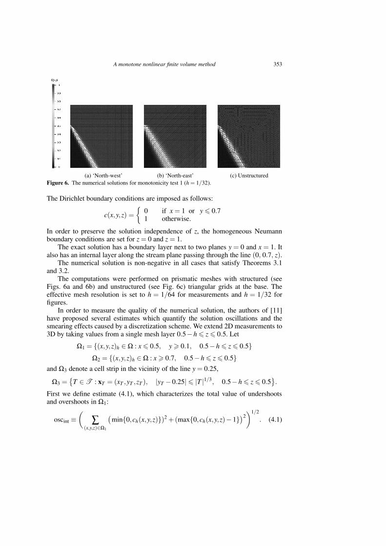
(a) ‘North-west’ (b) ‘North-east’ (c) Unstructured

Figure 6. The numerical solutions for monotonicity test 1 (h = 1/32).

The Dirichlet boundary conditions are imposed as follows:

c(x,y,z) =

0 if x = 1 or y 6 0.71 otherwise.

In order to preserve the solution independence of z, the homogeneous Neumannboundary conditions are set for z = 0 and z = 1.

The exact solution has a boundary layer next to two planes y = 0 and x = 1. Italso has an internal layer along the stream plane passing through the line (0, 0.7, z).

The numerical solution is non-negative in all cases that satisfy Theorems 3.1and 3.2.

The computations were performed on prismatic meshes with structured (seeFigs. 6a and 6b) and unstructured (see Fig. 6c) triangular grids at the base. Theeffective mesh resolution is set to h = 1/64 for measurements and h = 1/32 forfigures.

In order to measure the quality of the numerical solution, the authors of [11]have proposed several estimates which quantify the solution oscillations and thesmearing effects caused by a discretization scheme. We extend 2D measurements to3D by taking values from a single mesh layer 0.5−h 6 z 6 0.5. Let

Ω1 = (x,y,z)h ∈Ω : x 6 0.5, y > 0.1, 0.5−h 6 z 6 0.5

Ω2 = (x,y,z)h ∈Ω : x > 0.7, 0.5−h 6 z 6 0.5

and Ω3 denote a cell strip in the vicinity of the line y = 0.25,

Ω3 =

T ∈ T : xT = (xT ,yT ,zT ), |yT −0.25| 6 |T |1/3, 0.5−h 6 z 6 0.5

.

First we define estimate (4.1), which characterizes the total value of undershootsand overshoots in Ω1:

oscint ≡

(

∑(x,y,z)∈Ω1

(

min0,ch(x,y,z))2 +(max0,ch(x,y,z)−1

)2

)1/2

. (4.1)


Table 4.

‘North-west’ grid (see Fig. 6a), comparison of oscilla-

tions and smearing.

Name oscint oscexp smearint smearexp

SUPG 5.9e-1 2.1e-0 3.7e-2 5.6e-1MH85 6.1e-13 0 5.8e-2 1.1e-5FVMON 7.8e-8 1.6e-6 4.7e-2 1.7e-5

Table 5.

‘North-east’ grid (see Fig. 6b), comparison of oscilla-

tions and smearing.


SUPG 6.9e-1 3.8e-0 6.2e-2 1.7e-0MH85 0 0 1.0e-1 1.2e-5FVMON 2.1e-11 1.7e-7 1.1e-1 1.8e-5

Table 6.

Unstructured grids (see Fig. 6c), comparison of oscilla-

tions and smearing.


SUPG 5.9e-1 1.5e-0 5.5e-2 4.1e-1MH85 4.9e-15 1.8e-14 9.7e-2 5.3e-2FVMON 3.5e-6 5.0e-7 5.9e-2 2.2e-5

Second, we define estimate (4.2), which quantifies the oscillations near the boundarylayer in Ω2:

oscexp ≡

(

∑(x,y,z)∈Ω2

(

max0,ch(x,y,z)−1)2

)1/2

. (4.2)

Third, we define two estimates (4.3) and (4.4), which measure the thickness of theboundary layer and the internal shock, respectively:

smearexp ≡

(

∑(x,y,z)∈Ω2

(

min0,ch(x,y,z)−1)2

)1/2

(4.3)

smearint ≡ x2− x1 (4.4)

wherex1 = min

xT∈Ω3,C(xT )>0.1xT , x2 = max

xT∈Ω3,C(xT )60.9xT .

For the continuous solution these estimates depend only on the diffusion process,so they are much smaller than the considered mesh size. For the numerical solution,


Figure 7. The solution isolines in the xy-plane for the problem with the no-flow outer boundaryconditions.

Table 7.

The maximum concentration values for the problem with

the no-flow outer boundary conditions.

h 1/11 1/22 1/44 1/88

maxC 1.882 1.219 1.041 1.020

small values of estimates (4.1)–(4.4) characterize an almost non-oscillatory and al-most non-diffusive discrete solution. The smaller width of the internal shock andthe boundary layer in a numerical solution, the less smearing is introduced by thediscretization scheme.

The results obtained by the nonlinear FV, SUPG, and MH85 methods are shownin Tables 4, 5, and 6. Our method is competitive with the best 2D results presentedin review [11]. The increase in the internal shock width on the ‘north-east’ prismaticmesh is caused by the larger cell size in the direction normal to the ‘shock’.

At the second stage, we demonstrate that the FV discrete solution can violatethe DMP even on cubic meshes.

We extend the test case investigated in [1, 9] to the advection–diffusion equationby introducing a velocity field. We consider a unit cube with two vertical holes P1,

P2, Ω= (0,1)3 \(P1∪P2), Pi = Si×(0,1), i= 1,2, S1 = [3/11,4/11]× [5/11,6/11],S2 = [7/11,8/11]× [5/11,6/11]. The domain boundary is split into the outer partΓN where the homogeneous Neumann (no-flow) boundary condition is set, and twoinner parts ΓD,1, ΓD,2 where the Dirichlet boundary conditions are set: gD(x) = 0,x ∈ ΓD,1, gD(x) = 1, x ∈ ΓD,2.


The anisotropic diffusion tensor is

K = Rz(−θz)Ry(−θy)Rx(−θx)diag(k1,k2,k3)Rx(θx)Ry(θy)Rz(θz) (4.5)

where k1 = k3 = 1, k2 = 10−3, θx = θy = 0, θz = 67.5, and Ra(α) is the rotationmatrix in the plane orthogonal to oa with the angle α .

The velocity field is v = (10−2,10−2,0). According to the maximum principlefor elliptic PDEs the exact solution should be between 0 and 1 and have no extremaon the no-flow boundary ΓN .

The FV discrete solution on the cubic mesh with h= 1/32 is shown in Fig. 7. Itis non-negative in agreement with Theorem 3.2, but demonstrates overshoots nearthe no-flow boundary. These overshoots decrease rapidly as we refine the mesh, seeTable 7.

Conclusion

We have presented a new monotone finite volume method on polyhedral meshes forthe advection–diffusion equation with a piecewise continuous full anisotropic dif-fusion tensor and a piecewise continuous advection field. The method is the naturalextension of the 3D scheme for the diffusion equation [9] and the 2D scheme forthe advection–diffusion equation [26]. The numerical solution is non-negative, pro-vided that the source term and the Dirichlet boundary data are non-negative and theflux on the Neuman boundary is non-positive. The method does not require to inter-polate the solution to the mesh nodes and can be applied to unstructured polyhedralmeshes. The numerical experiments demonstrate the second-order convergence ratefor the concentration and the first-order convergence rate for the flux on randomlydistorted meshes in both advection-dominated and diffusion-dominated regimes.

References

1. I. Aavatsmark, G. Eigestad, B. Mallison, and J. Nordbotten, A compact multipoint flux approxi-mation method with improved robustness. Numer. Meth. Partial Diff. Equations (2008) 24, No. 5,1329–1360.

2. D. Benson, A new two-dimensional flux-limited shock viscosity for impact calculations. Comp.Meth. Appl. Mech. Engrg. (1991) 93, 39–95.

3. E. Bertolazzi and G. Manzini, A cell-centered second-order accurate finite volume method forconvection–diffusion problems on unstructured meshes. Math. Models Meth. Appl. Sci. (2004)14, No. 8, 1235–1260.

4. E. Bertolazzi and G. Manzini, A second-order maximum principle preserving finite volumemethod for steady convection–diffusion problems. SIAM J. Numer. Anal. (2005) 43, No. 5, 2172–2199.

5. A. N. Brooks and T. J. R. Hughes, Streamline upwind/Petrov–Galerkin formulations for convec-tion dominated flows with particular emphasis on the incompressible Navier–Stokes equations.Comp. Meth. Appl. Mech. Engrg. (1982) 32, No. 1–3, 199–259.

6. E. Burman and A. Ern, Discrete maximum principle for Galerkin approximations of the Laplaceoperator on arbitrary meshes. Comptes Rendus Mathematique (2004) 338, No. 8, 641–646.


7. G. Chavent and J. Jaffre, Mathematical Models and Finite Elements for Reservoir Simulation.Elsevier Science Publishers, B.V., Netherlands, 1986.

8. P. G. Ciarlet and P.-A. Raviart, Maximum principle and uniform convergence for the finite ele-ment method, Comp. Meth. Appl. Mech. Engrg. (1973) 2, 17–31.

9. A. A. Danilov and Yu. V. Vassilevski, A monotone nonlinear finite volume method for diffusionequations on conformal polyhedral meshes. Russ. Numer. Anal. Math. Modelling (2009) 24,No. 3, 207–227.

10. F. Gao, Y. Yuan, and D. Yang, An upwind finite-volume element scheme and its maximum-principle-preserving property for nonlinear convection–diffusion problem. Int. J. Numer. Meth.Fluids (2008) 56, No. 12, 2301–2320.

11. V. John and P. Knobloch, On spurious oscillations at layers diminishing (SOLD) methods forconvection–diffusion equations: Part I. A review. Comp. Meth. Appl. Mech. Engrg. (2007) 196,2197–2215.

12. M. E. Hubbard, Multidimensional slope limiters for MUSCL-type finite volume schemes onunstructured grids. J. Comp. Phys. (1999) 155, No. 1, 54–74.

13. T. J. R. Hughes, M. Mallet, and A. Mizukami, A new finite element formulation for computa-tional fluid dynamics. II. Beyond SUPG. Comp. Meth. Appl. Mech. Engrg. (1986) 54, 341–355.

14. I. Kapyrin, A family of monotone methods for the numerical solution of three-dimensional dif-fusion problems on unstructured tetrahedral meshes. Dokl. Math. (2007) 76, No. 2, 734–738.

15. S. Korotov, M. Krızek, and P. Neittaanmaki, Weakened acute type condition for tetrahedral tri-angulations and the discrete maximum principle. Math. Comp. (2001) 70, No. 233, 107–119(electronic).

16. D. Kuzmin, On the design of general-purpose flux limiters for finite element schemes, I. Scalarconvection. J. Comp. Phys. (2006) 219, No. 2, 513–531.

17. D. Kuzmin and M. Moller, Algebraic flux correction, I. Scalar conservation laws. In: Flux-Corrected Transport: Principles, Algorithms, and Applications (Eds. D. Kuzmin, R. Lohner,and S. Turek). Springer-Verlag, Berlin, 2005, pp. 155–206.

18. D. Kuzmin, M. J. Shashkov, and D. Svyatskiy, A constrained finite element method satisfyingthe discrete maximum principle for anisotropic diffusion problems. J. Comp. Phys. (2009) 228,No. 9, 3448–3463.

19. O. Ladyzhenskaya and N. Uraltseva, Linear and Quasilinear Elliptic Equations. Nauka,Moscow, 1973 (in Russian).

20. S. Lamine and M. G. Edwards, Higher-resolution convection schemes for flow in porous mediaon highly distorted unstructured grids. Int. J. Numer. Meth. Engrg. (2008) 76, No. 8, 1139–1158.

21. C. LePotier, Schema volumes finis monotone pour des operateurs de diffusion fortementanisotropes sur des maillages de triangle non structures. C. C. Acad. Sci., Paris (2005) 341,787–792.

22. C. LePotier, Finite volume scheme satisfying maximum and minimum principles for anisotropicdiffusion operators. In: (Eds. R. Eymard and J.-M. Herard). Finite Volumes for Complex Appli-cations V (2008), 103–118.

23. R. J. LeVeque, Finite Volume Methods for Hyperbolic Problems. Cambridge Univ. Press, Cam-bridge, 2002.

24. K. Lipnikov, D. Svyatskiy, M. Shashkov, and Y. Vassilevski, Monotone finite volume schemesfor diffusion equations on unstructured triangular and shape-regular polygonal meshes. J. Comp.Phys. (2007) 227, 492–512.


25. K. Lipnikov, D. Svyatskiy, and Y. Vassilevski, Interpolation-free monotone finite volume methodfor diffusion equations on polygonal meshes. J. Comp. Phys. (2009) 228, No. 3, 703–716.

26. K. Lipnikov, D. Svyatskiy, and Y. Vassilevski, A monotone finite volume method for advection–diffusion equations on unstructured polygonal meshes. J. Comp. Phys. (2010) 229, 4017–4032.

27. R. Liska and M. Shashkov, Enforcing the discrete maximum principle for linear finite elementsolutions of second-order elliptic problems. Commun. Comp. Phys. (2008) 3, No. 4, 852–877.

28. G. Manzini and A. Russo, A finite volume method for advection–diffusion problems inconvection-dominated regimes. Comp. Meth. Appl. Mech. Engrg. (2008) 197, No. 13–16, 1242–1261.

29. K. B. Nakshatrala and A. J. Valocchi, Non-negative mixed finite element formulations for atensorial diffusion equation, J. Comp. Phys. (2008) 228, No. 18, 6726–6752.

30. J. M. Nordbotten, I. Aavatsmark, and G. T. Eigestad, Monotonicity of control volume methods.Numer. Math. (2007) 106, No. 2, 255–288.

31. A. Quarteroni and A. Valli, Numerical Approximation of Partial Differential Equations.Springer-Verlag, Heidelberg, SCM Series No. 23, 1994.

32. V. Ruas Santos, On the strong maximum principle for some piecewise linear finite element ap-proximate problems of nonpositive type. J. Fac. Sci. Univ. Tokyo Sect. IA Math. (1982) 29, No. 2,473–491.

33. H. van der Vorst, Bi-CGSTAB: a fast and smoothly converging variant of Bi-CG for the solutionof non-symmetric linear systems. SIAM J. Sci. Stat. Comp. (1992) 13, No. 2, 631–644.

34. B. van Leer, Towards the ultimate conservative difference scheme. V. A second-order sequel toGodunov’s method. J. Comp. Phys. (1979) 32, No. 1, 101–136.

35. Yu. Vassilevski and I. Kapyrin, Two splitting schemes for nonstationary convection–diffusionproblems on tetrahedral meshes. Comp. Math. Math. Phys. (2008) 48, No. 8, 1349–1366.

36. D. Wollstein, T. Linss, and R. Hans-Gorg, Uniformly accurate finite volume discretization for aconvection–diffusion problem Electronic Transactions on Numer. Anal. (2002) 13, 1–11.

37. A. Yuan and Z. Sheng, Monotone finite volume schemes for diffusion equations on polygonalmeshes. J. Comp. Phys. (2008) 227, No. 12, 6288–6312.

A monotone nonlinear ﬁnite volume method for advection...

Documents

Transcript of A monotone nonlinear ﬁnite volume method for advection...