A Modern Macroeconomic Perspective - people.ucsc.eduhutch/Hutchison and Pasricha chap Ex Rate... ·...

Chetan Ghate ⋅ Kenneth M. KletzerEditors

Monetary Policy in IndiaA Modern Macroeconomic Perspective

Foreword by John B. Taylor

123

[email protected]

Exchange Rate Trends and Managementin India

Michael M. Hutchison and Gurnain Kaur Pasricha

1 Introduction

This chapter evaluates developments in India’s nominal and real exchange ratesover the past two decades, describing longer term trends as well as short-termmovements and volatility. Exchange rate movements are influenced by a host ofreal and nominal determinants, including government policy, especially foreignexchange market intervention, capital controls, and monetary policy. We explorehow these policies in India responded to exchange rate movements and how theyhave, in turn, influenced the exchange rate.

India has been developing its foreign exchange market and the average dailyturnover in the onshore market, sum of spot, and forward transactions, increasedtenfold in about 15 years—from 2.7 billion USD in March 1999 to about 30 billionUSD in March 2015.1 Rapid growth in the foreign exchange market reflects India’srise in international trade, especially in services, the broadening and deepening ofthe financial sector, and increasing globalization of the economy.

We would like to thank Bryce Shelton for excellent research assistance, and Rose Cunningham,Mark Kruger, and Errol D’Souza for helpful comments. The views expressed in this paper arethose of the authors. No responsibility for them should be attributed to the Bank of Canada.

M.M. Hutchison (✉)Department of Economics, University of California, Santa Cruz, CA 95064, USAe-mail: [email protected]

G.K. PasrichaInternational Economic Analysis Department, Bank of Canada, Ottawa, Canadae-mail: [email protected]

1Source: Reserve Bank of India, Database on the India economy. The numbers cited are the sum ofmerchant and interbank purchases and monthly averages of daily data.

© Springer India 2016C. Ghate and K.M. Kletzer (eds.), Monetary Policy in India,DOI 10.1007/978-81-322-2840-0_12

357

[email protected]

Maintaining orderly conditions in the foreign exchange markets is an officialobjective of the Reserve Bank of India (RBI).2 RBI is the manager of the ForeignExchange Regulation Act (FEMA, 2004), which also gives it the power to imposecapital controls.3 In practice, this objective has meant very active management ofcontrols on international capital movements and frequent foreign exchange marketintervention operations, as well as at least one episode of interest rate defense of theexchange rate in 2013.4 These considerations make understanding the linkagesbetween monetary policy, capital controls, and foreign exchange market interven-tion operations central to a study of exchange rates in India.

We begin in Sect. 2 with a statistical representation and analysis of the Rupeeexchange rate, comparing the bilateral rate against US dollar (USD) with thetrade-weighted multilateral nominal and real exchange rates. The bilateral exchangerate against the USD is the rate that the RBI monitors most closely and attempts tostabilize, through its interventions in the spot and forward markets. However, themultilateral rate is probably the most important, measured in real terms, for theIndian economy. Overall, the bilateral and multilateral measures point to largecumulative nominal depreciation of the rupee over January 1998–December 2014.Trend inflation in India over this period was much higher than inflation in the U.S.,however, resulting in substantial real (price-adjusted) appreciation of the rupeeagainst USD. By contrast, nominal trend depreciation of the rupee currency on amultilateral basis largely offset moderate inflation differentials between India and abroad index of its trading partners, leading to a fairly stable real multilateral realexchange rate—formal tests of long-term purchasing power parity (PPP) cannot berejected. Exchange rates by either measure have not moved uniformly since 1998,leading us to identify several distinct “regimes” during which exchange rate trendsand volatilities exhibited quite different patterns. Exchange rate volatility rosemarkedly in the mid-2000s, especially since the Global Financial Crisis (GFC).

Section three considers the policy levers that affect exchange rates—exchangerate management—and in particular whether foreign exchange market interventionand changes in the intensity of capital controls are consistent with, and directedtoward, an exchange rate objective. This section also considers how interventionand capital controls interact with monetary policy in navigating a balance betweenexternal and internal policy objectives. Section four concludes. We argue that the

2See for example, Khan (2011) which notes “Excessive volatility in exchange rate is a potentialsource of macroeconomic instability, and accordingly, the RBI aims at containing volatility toensure a stable macroeconomic environment.”.3Quotation from RBI website: https://www.rbi.org.in/scripts/FS_Overview.aspx?fn=5.4That is to say that the exchange rate enters into the RBI’s policymaking not only due to its impacton inflation but also its potential impact on economic growth directly and on financial stability. Incountries where central bank targets inflation (since 2015 for the RBI) and the central bankcredibility is high, exchange rate pass-through to inflation is typically low. Many advancedeconomies have seen the exchange rate pass-through decline over time (BIS, 2005), and centralbanks worry about exchange rate movements mainly to the extent that they affect current orexpected inflation.

358 M.M. Hutchison and G.K. Pasricha

[email protected]

gradual rise in financial openness in India has pushed the RBI to accept moreinstability in the exchange rate in favor of greater monetary independence.Monetary independence since the GFC has primarily focused on stimulating outputgrowth and employment, and not controlling inflation.

2 Nominal and Real Exchange Rates: Bilateraland Trade-Weighted Baskets

2.1 Trends

Chart 1 shows the development of two nominal exchange rate measures for theIndian rupee (INR) from January 1998 through December 2014: the U.S.Dollar/INR exchange rate and the INR against a trade-weighted basket of 36 tradingpartners.5 The base for each index is set as 100 for January 1998, and a decline inthe index represents a fall in the value of the rupee. Monthly data is shown.

Cumulative nominal depreciation in the USD/INR rate over January 1998–-December 2014 was about 40 %, while declining on a broad trade-weighted basisby almost 30 %. However, three phases in the nominal exchange rate are identifi-able from Chart 1, consistent across the two INR measures and denoted by verticallines: (a) a period of moderate fluctuations during 1998–2007, initially character-ized by gradual nominal depreciation until 2006, followed by robust appreciation;the result was quite similar exchange rate values in 1998 and early 2008; (b) aperiod of sharp depreciation and very high volatility from mid-2008 to mid-2013;(c) a period of relative stability since October 2013.

Measures of the real exchange rate, by contrast, reveal quite different longer-term patterns. Chart 2 shows the corresponding real USD/INR exchange rate andthe 36-country trade-weighted real multilateral exchange rate. The base is set to 100in January 2001 (sample is limited by data availability on relative prices). A rise ineach index implies a real exchange rate appreciation. We again distinguish the threenominal exchange rate episodes by vertical lines, contrasting nominal with realexchange rate developments. As is apparent, real exchange rate developments aremore difficult to classify than nominal exchanges into distinct phases and showsubstantial medium-term swings.

The indices demonstrate substantial cumulative real exchange rate appreciationagainst the U.S. Dollar over the 15-year period (more than 40 %). But against abroad basket of 36 currencies the INR has appreciated relatively little (9 %) and wasat virtually the same real value in September 2013 as early 2001. Strong realappreciation in 2014 pushed the real value of the 36-country weighted exchangerate again above its stable “Purchasing Power Parity” (PPP) value. Despite thelarger movements in real bilateral than trade-weighted index, the two series are

5See appendix A for data sources and descriptions.

Exchange Rate Trends and Management in India 359

[email protected]

highly correlated, with a correlation coefficient of 0.83 over the period January2001–December 2014. The nominal series, by contrast, have a correlation coeffi-cient of only 0.23 over the same period.

The divergent trends in nominal and real exchange rates are explained, of course,by relative price developments in India vis-à-vis the U.S. and vis-à-vis India’scounterparts in the currency baskets. Chart 3 shows two series—the relative Indian

40

60

80

100

120

1998 2000 2002 2004 2006 2008 2010 2012 2014

Index

Indian Rupee vis-à-vis US$

Nominal effective exchange rate -36 currency index

Index. January 1998 = 100Increase = Appreciation

Chart 1 Nominal exchange rate movements Sources U.S. Federal Reserve, Reserve Bank ofIndia, and Bank of Canada calculations

60708090100110120130140150160170

2001 2003 2005 2007 2009 2011 2013

Index

Real Indian Rupee vis-à-vis US$Real effective exchange rate -36 currency indexIndian Rupee vis-à-vis USD (Nominal)

Index: January 2001 = 100

Chart 2 Real exchange rate movements Sources Bloomberg, Reserve Bank of India, and Bank ofCanada calculations


[email protected]

price level against the U.S. and the relative Indian price level against atrade-weighted average of 36 countries. The chart shows that, since 2001, therelative Indian price level climbed more than 90 % compared to the U.S. price leveland almost 50 % against a broad price index of trading partners. The comparativelyrapid rise in the Indian price level explains why the USD/INR exchange rateappreciated by 42 % in real terms over this period despite an almost 30 % depre-ciation in the nominal exchange rate. By contrast, the modest 11 % real appreciationof the INR against the broad currency basket during 2001–2015 reflects the effect ofa 25 % nominal deprecation largely offsetting the larger rise in the Indian price levelrelative to its trading partners.

A few other noteworthy observations emerge during the subsamples. First, trendreal appreciation against the USD is evident in the second phase (mainly during2009–2012). This contrasts markedly with the relatively steady nominal exchangerate values during this period. Second, the substantial instability and volatility in thereal exchange rate with alternating bouts of depreciation followed by rebounds isparticularly noteworthy in the second phase. Movements in the real USD/INR ratewere greatest, with a real value index of 138 in December 2007, falling to a low of115 in February 2009 and then sharply appreciating to 162 by July 2011. Sub-stantial depreciation again followed, reaching 128 by August 2013. The realtrade-weighted index followed a similar pattern, but with less extreme movements,ending this episode (August 2013) with about a 10 % cumulative real depreciationagainst the broad (36 country) multilateral index. Third, the final episode in oursample, August 2013 through January 2015, showed substantial real appreciation.

80

100

120

140

160

180

200

2001 2003 2005 2007 2009 2011 2013

Index

Real price differential between U.S. and India CPI

Real Indian Rupee vis-à-vis US$

Index: January 2001 = 100

Chart 3 Relative price movements Sources U.S. Bureau of Labor Statistics, India Ministry ofStatistics and Programme Implementation, Reserve Bank of India, and Bank of Canadacalculations


[email protected]

2.2 Volatility

Chart 4 shows that high volatility and turbulence in the INR during 2008–2013 isquite distinct compared with the relative stability of the two other periods. Gen-erally, month-to-month fluctuations in the INR/USD rate over most of the samplehave been within a ±2.5 % band. The exchange rate volatility increased post-2004,but the volatility of the Global Financial Crisis and its aftermath—characterized bya higher frequency of days exceeding the 2.5 % ± band—is clearly distinct fromthe other periods. The volatility of the nominal trade-weighted index also increasedbetween 2008 and 2013, but the shift is not as dramatic as for the INR/USD spotrate.

Though volatility of the INR/USD was relatively high compared to the broadtrade-weighted index, it was comparatively low compared to the two other mostactively traded and heavily weighted (in the broad currency basket) internationalcurrencies in the index—the British pound (GBP) and the euro. This reflects theRBI’s focus on mitigating volatility in the INR/USD rate over much of the period.Chart 5 plots the annualized volatility of the INR spot exchange rate against theUSD, the GBP, and the euro. These are computed as the annualized volatility of thedaily percentage spot exchange rate changes in the month, and smoothed by takingthe lagged 6-month moving average. The chart shows that, through the end of 2006,volatility of the INR/USD pair was much lower than that of INR against these twoother major international currencies. Although other factors were at work, thispattern is consistent with central bank actions attempting to mitigate INR/USDvolatility. However, post-2007, and particularly between 2008 and 2013, volatility

-10

-5

0

5

10

1998 2000 2002 2004 2006 2008 2010 2012 2014

%

Nominal effective exchange rate -36 currency index

US$ vis-à-vis Indian Rupee

+/-2 per cent band

Month-over-month percentage change

Chart 4 Monthly percentage change in nominal exchange rates Sources Bloomberg and authors’calculations


[email protected]

in the INR/USD was closer to the volatility of INR against the GBP and the euro,suggesting limited intervention (or limited effectiveness of such intervention).

In terms of real exchange volatility, shown in Chart 6, both bilateral and mul-tilateral indices show substantial fluctuations over the sample period, frequentlyexceeding the ±2.5 % band. There are two similarities between the nominal

0

5

10

15

20

1998 2000 2002 2004 2006 2008 2010 2012 2014

%

Indian Rupee vis-à-vis US$Indian Rupee vis-à-vis the EuroIndian rupee vis-à-vis British Pound

Monthly volatility of daily spot exchange rate changes, 6-month moving average

Chart 5 Annualized Volatility of Rupee spot exchange rates Sources Datastream, Reserve Bankof India, and Bank of Canada calculations

-10

-5

0

5

10

1998 2000 2002 2004 2006 2008 2010 2012 2014

%

Real Indian Rupee vis-à-vis US$Real effective exchange rate -36 currency index+/-2 per cent band

Month-over-month percentage change

Chart 6 Monthly percentage change in real exchange rates Sources Bloomberg, Reserve Bank ofIndia, and Bank of Canada calculations


[email protected]

exchange rate volatilities (Chart 4) and real exchange rate volatilities (Chart 6). Aswith nominal exchange rates, volatility was greatest for real exchange rate duringthe GFC and its aftermath (2008–2013). Nominal and real exchange rate volatilityagainst USD has also been larger than that against the trade-weighted basket ofcurrencies. The main difference between the nominal and real exchange ratevolatilities is that real exchange rate volatility was relatively higher even in thepre-2006 period, with frequent deviations outside the ±2.5 % band.

2.3 Long-Term Linkages Between Prices and ExchangeRates: PPP and Cointegration Tests

The descriptive analysis indicates the Indian real exchange rate against the USD hasshown a much larger trend appreciation, and greater volatility, than against a broadbasket of currencies. These observations are borne out by formal cointegration testswhere we investigate whether purchasing power parity (PPP) holds in the longerterm. This procedure amounts to testing for a long-term linkage (cointegration)between the (log) nominal exchange rate and (log) relative prices. Formal PPPwould indicate a 1:1 long-term (negative) linkage between the nominal exchangerate and relative prices. However, we postulate a weaker relationship, testingwhether a cointegrating vector exists between the nominal exchange rate and rel-ative price, allowing for a linear trend as a deterministic variable. We consider boththe Granger–Engle and the Phillips–Ouliaris (residual) tests of cointegration andreport both the tau-statistic and the Z-statistic. The null is that the nominal exchangerate and relative prices are not cointegrated, hence rejecting the null indicates along-run relationship between the two series.

Table 1 reports the results of the cointegration tests for the USD/INR exchangerate and the Indian/US relative CPI price. Table 2 reports the results between the

Table 1 Cointegration between nominal INR/USD exchange rate and relative CPI

Variable Coefficient Standard error t-Statistic Probability

Constant 0.073 0.021 3.523 0.001Log(RPRICE_IND_US) −0.416 0.063 −6.582 0.000R2 54.9Adjusted R2 54.6Null hypothesis: series are not cointegrated

Value Probabilitya

Engle–Granger tau-statistic 0.549 0.694Engle–Granger Z-statistic 0.546 0.660Phillips–Ouliaris tau-statistic 0.078 0.670Phillips–Ouliaris Z-statistic 0.028 0.634aMacKinnon (1996) p-values


[email protected]

broad multilateral exchange rate index and the Indian price level vis-à-vis theforeign country weighted price index. The first part of each table reports the pointestimates of the long-run relationship (using fully modified least squares), includinga constant term and linear trend, and the second part reports the formal cointe-gration tests on the residual series.

Comparing the point estimates across the two series, it is evident that the linkageof relative Indian price level bilaterally against the USD is much weaker thanagainst the multilateral basket of currencies, i.e., the point estimate of the former is−0.42 (USDINR rate depreciates only 0.42 % in response to a 1 % rise in relativeprice level in India relative to U.S.) and the point estimate of the latter is −0.82(trade-weighted nominal exchange rate depreciates 0.82 % in response to a 1 % risein relative price level in India relative to group of trading partners). However, thestrict PPP restriction of −1.0 as a cointegrating term is decisively rejected for bothequations at the 1 % level of significance. In line with observations of volatility, thelong-run variance estimate against the USD is much larger than against the basketof currencies.

Not surprisingly, the weaker test of cointegration (any stable longer-term link,not necessarily 1:1) is strongly rejected between exchange rates and prices in Indiaand the U.S. by both the Granger–Engle and Phillips–Ouliaris tests (Table 1).Trend movements in the USD/INR exchange rate simply do not reflect longer termmovements in relative prices between the two countries.

Cointegration is not rejected, however, between relative prices and the multi-lateral exchange rate (Table 2). Three of the test statistics reject the “no cointe-gration” null at the 5 % level of significance, and the fourth rejects at the 6 % level.This is strong descriptive and statistical evidence that longer term trends in theIndian nominal exchange rate, measured as a weighted average of a large group oftrading partners, reflects relative movements in price levels. It appears that a weakform of PPP holds, meaning that the real exchange rate for a broad basket ofcurrencies shows large fluctuations over the short- and medium-term horizons but

Table 2 Cointegration between nominal rupee trade-weighted (36 countries) exchange rate andrelative prices

Variable Coefficient Standard error t-Statistic Probability

Constant 4.621 0.006 822.186 0.000Log(RPRICE36) −0.828 0.038 −21.818 0.000R2 88.5Adjusted R2 88.5Null hypothesis: series are not cointegrated

Value Probabilitya

Engle–Granger tau-statistic −3.371 0.058Engle–Granger Z-statistic −21.911 0.043Phillips–Ouliaris tau-statistic −3.528 0.039Phillips–Ouliaris Z-statistic −23.991 0.027aMacKinnon (1996) p-values


[email protected]

reverts to a stable trend over longer periods—the nominal exchange rate largelyadjusts (about 82 % of the movement) to offset relative price movements overlonger periods.

3 Exchange Rate Policy: Intervention, Capital Controls,and Monetary Policy

Although long-term movements in the INR exchange rate may largely reflect rel-ative price trends between India and its trading partners, as well as real factors suchas relative productivity developments and other “real” shocks, short-andmedium-term fluctuations are influenced by a host of factors including govern-ment policy, especially foreign exchange market intervention, capital controls andmonetary policy.

The objectives of an exchange policy are typically multifaceted, but generallyfocus on mitigating exchange rate volatility and turbulence as well as influencingthe medium-term path of the exchange rate. However, the mix of policies is alsoconstrained by the “trilemma” which suggests limits to independent policies acrossthree dimensions: exchange rates, external capital controls (financial openness), andmonetary policy. We explore how different dimensions of policy in India may haveinfluenced the exchange rate. In what follows, we discuss intervention, capitalcontrols, and monetary policy as they relate to capital inflows and exchange rates.

Mitigating exchange rate volatility has been an explicit objective of the ReserveBank of India (RBI) for decades, long acknowledged in official documents andspeeches.6 RBI is also the manager under the Foreign Exchange Management Act(FEMA) 1999, which gives it the objective of “promoting the orderly developmentand maintenance of foreign exchange market in India” and the powers to restricttransactions in foreign currency.7 In consultation with the government, the RBI mayspecify the class of capital account transactions that are permissible and the limit upto which foreign exchange can be made available for these transactions. Further, theRBI has broad powers to issue regulations to prohibit, restrict, and regulate trans-actions between residents and nonresidents in securities, lending, immovable

6For example, page 15 of RBI’s (2014) Annual report states that RBI’s response to the devel-opments following the US Fed’s indication that it would taper its large-scale asset purchaseprogram “aimed at containing exchange rate volatility, compressing the current account deficit(CAD) and rebuilding buffers.”.7FEMA 1999 was passed to replace the Foreign exchange Regulation Act, (FERA) 1973 (lateramended as FERA 1993). FERA 1973 was a draconian law that made violation of foreignexchange regulations a criminal offense and presumed guilty until proven innocent. In addition toreversing these provisions of the FERA and other liberalizations, the FEMA 1999 also made therupee convertible on the current account. However, the RBI and the Government of India con-tinued to have the power to regulate transactions on both current and capital account and themarket for foreign exchange. The full text of the act is available here: http://finmin.nic.in/the_ministry/dept_eco_affairs/capital_market_div/FEMA_act_1999.pdf.


[email protected]

property, deposits, and currency notes. The RBI used capital controls as well asforeign exchange intervention to stabilize the exchange rate or to lean against thewind, to give some room to monetary policy responsive to domestic conditions.However, the constraints of the trilemma seemed to bind to some degree for theentire sample period, limiting monetary policy autonomy.

3.1 Exchange Rate Policy and Intervention

The policy shifts between maintaining exchange rate parities and allowing flexi-bility are evident throughout our sample period, with the RBI choosing differentconfigurations over time. Considerably more exchange rate variation is evident inrecent years, caused partly by the nature of the domestic and external environment(i.e., larger and more variance in external shocks) and partly by gradually openingof the external financial flows and willingness of the authorities to allow greaterexchange rate flexibility as a “shock absorber” to external shocks.

Greater financial openness and flexibility in exchange rates has also beenencouraged by the IMF. For example, the 2013 IMF Article IV Consultation Reportlauds the virtues of exchange rate flexibility and states that: “The floating Rupee isan important shock absorber. Rupee flexibility has offset inflation differentials andprevented exchange rate misalignment. Such flexibility would be particularlyimportant in case of renewed global financial stresses.” (IMF 2013, p. 20).8 Poli-cymakers allowing greater flexibility in recent years are consistent with the evi-dence in the Sect. 2 on how exchange rate depreciation is offsetting high inflationrates in India compared with its trading partners, Similarly, even in the face of quitehigh exchange rate volatility following the GFC and its aftermath, the 2015 IMFArticle IV Report states: “Given India’s increased and adequate reserve buffers,greater exchange rate flexibility would be welcome and thereby encourage privatesector entities to limit excessive risk taking. Foreign exchange intervention shouldbe limited to preventing disruptive movements in the exchange rate. If globalfinancial market volatility resurfaces, exchange rate flexibility should be animportant shock absorber.” (IMF 2015, p. 21).

Although the Indian authorities may accept greater exchange rate flexibility, theauthorities have nonetheless continued to engage in extensive interventions in theforeign exchange market. Chart 7 shows the accumulation of foreign exchangereserves in India from the RBI database and measured in (monthly) flows in billionsof USD. This is a measure of foreign exchange intervention, with increases rep-resenting purchases of USD in the foreign exchange market and decreases repre-senting sales of USD in the foreign exchange market. Generally, purchases ofdollars (sales of INR) by the RBI in the foreign exchange market are designed to

8The reports are not always consistent in the views expressed about the merits of exchange rateflexibility, however.


[email protected]

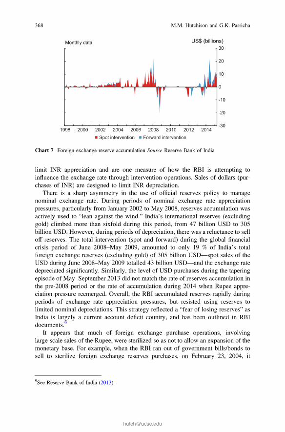
limit INR appreciation and are one measure of how the RBI is attempting toinfluence the exchange rate through intervention operations. Sales of dollars (pur-chases of INR) are designed to limit INR depreciation.

There is a sharp asymmetry in the use of official reserves policy to managenominal exchange rate. During periods of nominal exchange rate appreciationpressures, particularly from January 2002 to May 2008, reserves accumulation wasactively used to “lean against the wind.” India’s international reserves (excludinggold) climbed more than sixfold during this period, from 47 billion USD to 305billion USD. However, during periods of depreciation, there was a reluctance to selloff reserves. The total intervention (spot and forward) during the global financialcrisis period of June 2008–May 2009, amounted to only 19 % of India’s totalforeign exchange reserves (excluding gold) of 305 billion USD—spot sales of theUSD during June 2008–May 2009 totalled 43 billion USD—and the exchange ratedepreciated significantly. Similarly, the level of USD purchases during the taperingepisode of May–September 2013 did not match the rate of reserves accumulation inthe pre-2008 period or the rate of accumulation during 2014 when Rupee appre-ciation pressure reemerged. Overall, the RBI accumulated reserves rapidly duringperiods of exchange rate appreciation pressures, but resisted using reserves tolimited nominal depreciations. This strategy reflected a “fear of losing reserves” asIndia is largely a current account deficit country, and has been outlined in RBIdocuments.9

It appears that much of foreign exchange purchase operations, involvinglarge-scale sales of the Rupee, were sterilized so as not to allow an expansion of themonetary base. For example, when the RBI ran out of government bills/bonds tosell to sterilize foreign exchange reserves purchases, on February 23, 2004, it

-30

-20

-10

0

10

20

30

1998 2000 2002 2004 2006 2008 2010 2012 2014

US$ (billions)

Spot intervention Forward intervention

Monthly data

Chart 7 Foreign exchange reserve accumulation Source Reserve Bank of India

9See Reserve Bank of India (2013).


[email protected]

announced the launch of a market stabilization scheme to issue additional gov-ernment bills/bonds explicitly as sterilization instruments.10 At the peak, reservepurchases (both spot and forward) were about 22 billion USD a month in 2007.However, during the 2008 global financial crisis, foreign exchange reserves werenot used to stabilize a depreciating exchange rate, with sales being negligible.During 2009, the reserves accumulation resumed in periods of appreciation pres-sures, but compared to the pre-2008 period, the extent of accumulation remainedsubdued, until picking up again in 2014.

In summary, intervention policy in India has been mainly one-sided, directedtoward limiting exchange rate appreciation, during which times dollar purchaseswere generally large, and not directed toward limiting depreciation. The generaltrend in exchange rate depreciation in nominal terms over our sample period wasfacilitated by intervention policy. This policy may have allowed relative stability inthe real exchange rate, hence maintaining India export competitiveness, as theexchange rate depreciated over longer periods to offset relative high inflation inIndia. Intervention policy and exchange rate depreciation also allowed greatermonetary autonomy, especially during a period associated with increased financialliberalization of the international capital account. Moreover, reserve accumulation—through USD purchases on the foreign exchange market—is a desirable objectiveto the extent that it provides a stock of precautionary reserves in the event of abalance of payments/currency crisis or sudden stop in private capital inflows thatgenerally finance persistent current account deficits in India. On the other hand, theexchange rate did not play the role of a “nominal anchor” of monetary policy andhigh inflation in India as a consequence has been a recurring problem.

3.2 Capital Controls and Exchange Rates

Control of international financial capital movements is another policy instrumentthat has been frequently employed to influence financial flows in and out of Indiaand the exchange rate. Although the overall trend was toward financial liberaliza-tion of the capital account, capital control actions (i.e., tightening and easing ofrestrictions on capital flows) have been actively used as an instrument to “leanagainst the wind” of exchange rate pressures in both directions.

A measure of cumulative changes in the capital account is shown in Chart 8.These data are from Pasricha et al. (2015). Each of the capital account opennessindices is the cumulative sum of the number of weighted capital control easings lesstightenings per quarter. The changes are weighted by the share of the country’sinternational balance sheet that the measures are designed to impact (The weights

10See RBI announcement at: https://www.rbi.org.in/scripts/BS_PressReleaseDisplay.aspx?prid=9788.


[email protected]

are from Lane and Milesi-Ferretti). Four indices are shown: cumulative changes foreasings less tightenings for total capital inflows (outflows) and the total less FDI.

Chart 8 shows that both inflow and outflow restrictions have been graduallyliberalized. However, there were some reversals in the inflow liberalization process,and the timing of the actions on both inflow and outflow sides appear to be asso-ciated with the major changes in nominal exchange rate trends:

• There are two periods during which inflow liberalization trend was temporarilyreversed through a net tightening of inflow controls—2003–2004 and2006–2008.11 Both these were periods of appreciating nominal INR/USDexchange rate. These periods also saw several net liberalizations of outflowcontrols, as authorities attempted to reduce exchange rate appreciation pressureassociated with surging net capital inflows.

• There was significant net liberalization of inflow controls after 2008, particularlyduring 2008, 2011, and 2013, the years that saw sharp depreciations of theRupee. The year 2013 also saw tightening of outflow controls in response to thenet capital outflow pressures, as authorities responded to the taper tantrum.

0

2

4

6

8

10

12

14

16

18

2001 2003 2005 2007 2009 2011

Policy actions

Inflow Liberalization, weighted Outflow Liberalization, weighted

Number of policy actions, cumulated

Chart 8 Capital control liberalization in India Notes Each of the capital account openness indicesis the cumulative sum of number of (unweighted or weighted) capital control easings lesstightenings per quarter. The changes are weighted by the share of the country’s internationalbalance sheet the measures are designed to impact. The weights are from Lane and Milesi-Ferretti(2007), as in Pasricha et al. (2015). Source Pasricha et al. (2015)

11The de-jure liberalization resulted in de facto liberalization, as measured by deviations fromcovered interest parity. Hutchison et al. (2012b) use a self-Exciting Threshold Auto-Regressive(SETAR) model to the interest differentials between the onshore interbank rate and offshore-NDFimplied (covered) yield over the period 1998–2011 and find that prior to 2008, capital controltightenings were able to create a wedge between the offshore and onshore interest rates, but only inperiods in which the controls were actively tightened (March 2003–August 2005 and August2006–October 2008). They also find that post-2008, the no-arbitrage band for the differentials fellto close to zero.


[email protected]

The issue of whether changes in capital inflow controls in India systematicallyresponded to exchange rate pressures is addressed directly using an event studymethodology by Pandey et al. (2015). A figure from their work is shown as inChart. 9. This study finds that the 68 episodes of net capital inflow easing aresystematically associated with periods of INR exchange rate depreciation (risingINR/USD four weeks prior to changes in controls) and the 8 episodes of net capital

-5.0

-2.5

0.0

2.5

5.0

-12 -10 -8 -6 -4 -2 0

%

Event time (weels)Indian Rupee vis-à-vis US$ fluctuations prior to dates of CCAs95th percentile confidence interval

-7.5

-5.0

-2.5

0.0

2.5

-12 -10 -8 -6 -4 -2 0

%

Event time (weeks)Indian Rupee vis-à-vis US$ fluctuations prior to dates of CCAs95th percentile confidence interval

(a)

(b)

Easing events

Tightening events

Chart 9 a Capital controls responded to exchange rate pressures Note Sample includes 68 easingevents. Source Pandey et al. (2015), b Capital controls responded to exchange rate pressures NoteSample includes 8 tightening events. Source Pandey et al. (2015)


[email protected]

inflow tightening are associated with periods of INR appreciation (fall INR/USDten weeks prior to changes in controls). This suggests that the timing of changes incapital controls was influenced by the movements in exchange rate.

While capital controls on both inflows and outflows were used to respond tonominal exchange rate pressures, it is not clear that these measures delivered onreversing the exchange rate trend or even stabilizing it. Pandey et al. (2015) alsoaddress this issue. They employ a propensity score matching methodology to assessthe causal impact of changes in a certain type of inflow controls (those on foreignborrowing by Indian residents) for the period from January 2004 to September2013. The propensity score matching methodology controls address selection biasthat would arise in a simple event study or regression if policymakers use capitalcontrols for exchange rate management purposes. The weeks in which capitalcontrol actions (CCAs) were implemented will differ in identifiable ways, fromweeks in which CCAs were not implemented.

The propensity score matching (PSM) methodology is a way of building thecounterfactual of what would have happened if the controls had not been employed.Instead of trying to model the outcome variables, the methodology shifts focus tomodeling the policy variable (the use of a CCA) and estimating the conditionalprobabilities for the use of CCAs. These conditional probabilities, called propensityscores, are used to identify time periods that had similar characteristics to thoseprior to the date of the CCA but where no CCA was employed (control group). Thebehavior of the outcome variables for the control group gives a counterfactual forhow each of these variables would have behaved had the CCA not been employed.Outcomes of the weeks after the CCA are compared between the treatment andcontrol groups.

Chart 10, which is an updated version of the one in Pandey et al. (2015), plotsthe difference between nominal INR-USD spot exchange rate between treatmentand control weeks for easing of capital controls on foreign borrowing. It shows nosignificant difference between the outcomes after easing CCAs and the outcomes incontrol periods. This result also held for other outcome variables. Therefore, theyconclude that these controls did not significantly impact either nominal or realexchange rate movements.

Pandey et al. consider a longer sample, but one interesting episode is the periodof “taper tantrum,” May–September 2013. The taper tantrum began after Ber-nanke’s testimony to the US congress on May 22, 2013 that the Federal Reserve“could take a step down in our pace of purchase” of assets under the QE program,conditional on improving economic conditions.12 These events led to considerablemarket volatility and a global retrenchment from risk taking, with market

12The FOMC press conference in June further reiterated that the asset purchases could slow in thefall of 2013, conditional on the economic recovery continuing to take hold.


[email protected]

participants interpreting the statements to suggest that the Federal Reserve may startnormalizing policy earlier than markets had so far expected.

This retrenchment from risk-taking hit India particularly hard, as at that time theeconomic fundamentals appeared to be weak, with slowing growth, high inflation,high fiscal deficit, and political uncertainty due to the upcoming 2014 generalelections. The Indian policy response consisted of tightening of monetary policy,curbs on gold imports and currency trading, and liberalization of inflow controls.However, the Rupee depreciation continued unabated (Chart 11, Panel-a). TheRupee’s value hit the lowest among the other emerging markets that formed the“fragile five,” i.e., Brazil, Indonesia, South Africa, and Turkey (Chart 11, Panel-b).All the fragile five countries responded by raising interest rates, while Indonesia,Brazil, and Turkey also intervened in the currency markets. Sahay et al. (2014)assessed the domestic policy responses in an event study specification and foundthat EME policies during the taper tantrum did have a dampening effect on the paceof depreciation. However, the taper tantrum was officially over—and all the fragilefive currencies stabilized—only when the Federal Reserve did not reduce itsmonthly purchases under QE in its September 18 monetary policy announcement.

The upshot of this analysis is that a general trend of international capital marketliberalization has occurred in India, particularly on the liberalization of capitalinflows. Moreover, the intensity of liberalizations coincided with bouts of exchangerate pressure, such as the taper tantrum episode, with changes in capital controls

-2

-1

0

1

2

3

-4 -2 0 2 4

%

Event time (weeks)Cumulative difference of Indian Ruppe vis-à-vis US$ returns

95th percentile confidence interval

Chart 10 Causal impact of capital controls on nominal INR-USD exchange rate Source Pandeyet al. (2015)


[email protected]

attempting to moderate exchange rate movements. However, it is not clear from theempirical evidence that capital control changes had much impact on exchange ratemovements.

75

80

85

90

95

100

105

May 1 May 22 Jun 12 Jul 3 Jul 24 Aug 14 Sep 4 Sep 25

US$

Indian Rupee vis-à-vis US$

Index: 2 May 2013 = 100

a. 22-05-2013 -Bernanke Congressional Testimonyb. 06-06-2013 -Restrictions placed on gold importsc. 11-06-2013 -Curbs on exporter freedomd. 25-06-2013 -Restrictions placed on gold imports and easing of restrictions on ECB e. 08-07-2013 -Proprietary trading ban in currency markets onf. 15-07-2013 -Interest rate defence and easing of restrictions on ECBg. 22-07-2013 -Restrictions placed on gold importsh. 06-08-2013 -Raghuram Rajan appointed Governor of the RBIi. 13-08-2013 -Restrictions placed on gold importsj. 18-08-2013 -Easing of restrictions on ECBk. 28-08-2013 -RBI introduces forex swap window for public sector oil marketing companies

A B CD E F G H I J K

75

81

87

93

99

105

5-2-2013 6-2-2013 7-2-2013 8-2-2013 9-2-2013 10-2-2013Brazilian Real to US $ Indian Rupee to US $ South Africa Rand to US $Indonesian Rupiah to US $ New Turkish Lira to US $ FOMC Meeting (No Taper)

Index: 2 May 2013 =100(b)

(a)

Chart 11 a Capital controls and INR-USD exchange rate during “taper tantrum” a 05-22-2013—Bernanke Congressional Testimony, b 06-06-2013—Restrictions placed on gold imports,c 06-11-2013—Curbs on exporter freedom, d 06-25-2013—Restrictions placed on gold importsand easing of restrictions on ECB, e 07-08-2013—Proprietary trading ban in currency markets on,f 07-15-2013—Interest rate defense and easing of restrictions on ECB, g 07-22-2013—Restrictionsplaced on gold imports, h 08-06-2013—Raghuram Rajan appointed Governor of the RBI,i 08-13-2013—Restrictions placed on gold imports, j 08-18-2013—Easing of restrictions on ECB,k 08-28-2013—RBI introduces forex swap window for public sector oil marketing companiesSource Reserve Bank of India and Bank of Canada calculations, b Fragile 5 currencies during the“taper tantrum” Source Datastream


[email protected]

3.3 Monetary Policy, the Trilemma, and Exchange RateManagement

Monetary policy in India, especially the use of policy interest rates, has occa-sionally been influenced by external developments as well as directed towardmoderating exchange rate movements (Hutchison et al. 2012, 2013). The trade-offsbetween an independent interest rate (monetary) policy, exchange rate stability, andfinancial openness (deregulation of capital controls)—the well-known trilemmaconstraint—is clearly evident in India. The trilemma configuration is an importantpart of an analysis of factors determining exchange rates in India as exchange ratestability is compromised (given a particular external environment) when authoritiespursue greater capital market openness (financial liberalization) or follow an interestrate policy that diverges from the rest-of-the-world (monetary independence).

Policy constraints between these three policy instruments were operating in Indiaover the past decade, as shown in Chart 12. The chart shows the evolution ofinterest rate policy independence (monetary policy autonomy, MPA), internationalcapital account openness (KO), and exchange rate stability (ES). The monetarypolicy autonomy index (MPA) is computed as in Aizenman et al. (2008). Thisindex measures the inverse of the correlation between nominal money marketinterest rates in India and the US, and varies between 0 and 1, with higher valuesindicating greater monetary policy autonomy.13 The exchange rate stability index isalso computed as in Aizenman et al. (2008), as the normalized annual standarddeviation of the monthly percentage changes in nominal INR/USD spot exchangerate. To measure capital account openness (KO), we compute the index as the sumof total financial assets and liabilities as percentage of GDP.14

The MPA index suggests very low monetary policy autonomy during1999–2006, taking values below 0.3 for the entire period. The MPA index isdeclining from 1999 to 2004, a period when the volatility of exchange rate againstthe USD was lowest, as seen in Chart 2.15 This period is also characterized byheavy foreign exchange market purchases of USD, leading to large reservesaccumulation. Up to 2003, RBI sterilized the reserves purchases using open market

13We use IFS data on money market interest rates, where available, and monthly average ofinterest rates. For the US, this series is the federal funds rate. For India, the IFS series on moneymarket rates is missing between June 1998 and April 2006. For this period, we use the MIBORdata from Haver’s EMERGE database.14Exchange rate data is the monthly average nominal spot exchange rate against the USD seriesfrom IMF IFS. International investment position data is also from IMF IIP statistics.15The monetary policy autonomy index is based on money market interest rates, rather than actualpolicy rates. The RBI was reducing interest rate and cash reserve ratios over the period 1999–2004.However, sterilized intervention increased the supply of domestic bonds held by the public, whichmay have prevented full transmission to market interest rates. Real rates also did not decline in thisperiod as inflation was low (fiscal policy was contractionary, with declining fiscal deficit). Theindex therefore seems to capture well the declining monetary policy autonomy over the period ofsterilized intervention.


[email protected]

operations. In 2003, RBI ran out of government bonds with which to sterilize andthe government of India issued special market stabilization scheme bonds to ster-ilize intervention. As the fiscal cost of sterilization became more apparent under theMSS, this may have led to a slowdown in the rate of sterilization. The year 2004also marks the lowest point in the MPA index, after which it started increasing, asRBI shifted the focus from sterilized intervention to using more capital controls(tightening of controls on foreign borrowing and easing of outflow controls), aswell as gradually allowing (or accepting) more exchange rate volatility.

The year 2008 marked a shift in nominal exchange rate volatility, seen inChart 2 and measured by lower values of the exchange rate stability index ofChart 12. This allowed the authorities to maintain a high degree of monetary policyautonomy despite increasing capital account openness. The MPA index was fairlystable at around 0.5 in 2007–2010, climbing somewhat from in 2011–2012. Theexchange rate stability index continued to fall continuously from the mid- tolate-2000s and, by 2012, reached a level below that observed in late 1990s. A smalldecline in monetary policy autonomy is evident in 2013, as the RBI reacted to tapertantrum by an interest rate defense, intervention in spot, and forward markets aswell as capital controls.

To provide a sense of how the three policies: monetary, capital controls, andintervention were used to manage the exchange rate, Table 3 puts together the threepolicies and the trends in nominal exchange rate of the rupee against the USD forour sample period January 1, 1998–December 31, 2014. We divide the sampleperiod into 6 subperiods, based on the direction of monetary and capital controlspolicies. Specifically, we use capital control regime change dates identified byHutchison et al. (2012a) and update these beyond 2011, together with our judge-ment of the monetary policy cycle turning points (based on information on the

0

25

50

75

100

1998 2000 2002 2004 2006 2008 2010 2012 2014

Index

Monetary independence Exchange rate stability

Capital account openness

Chart 12 Trilemma indices for India Source Haver (IMF IFS and EMERGE databases) and theauthors’ calculations


[email protected]

Tab

le3

Policyregimedescription

Begin

End

Exchang

erate

trend

Regim

eDescriptio

nCapitalcontrols

Mon

etarypo

licy

Total

interventio

n(Spo

t+

Forw

ard)

Janu

ary1,

1998

July

7,20

03Depreciationup

toJan02

,then

appreciatio

n

MP:

Easing

Slow

andtentative

liberalizationof

inflo

ws

butfew

changes

Easing,

onall4

policyrates

USD

42billion

sCC:

SomeNKI

increasing

measures

Interventio

n:Yes,

purchases

July

8,20

03Octob

er10

,200

8App

reciation—

mod

erateup

toApril20

06,then

rapid

MP:

Neutral/Tight

Outflo

wlib

eralizations

andnettig

hteningof

restrictions

oninflo

ws,

particularly

between

2006

and20

08

Tightening,

startin

gin

Aug

ust20

04with

CRR

and

Octob

er20

05in

repo

rate

USD

149billion

s

CC:NKI

redu

cing

measures

Interventio

n:Yes,

purchases

Octob

er11

,20

08Nov

ember

20,2

009

Depreciation

MP:

Easing

Inflo

wlib

eralizations,

nochange

inou

tflow

controls

Easing

(Sales)USD

30billion

CC:NKI

increasing

measures

Interventio

n:Yes,sales

(con

tinued)


[email protected]

Tab

le3

(con

tinued)

Begin

End

Exchang

erate

trend

Regim

eDescriptio

nCapitalcontrols

Mon

etarypo

licy

Total

interventio

n(Spo

t+

Forw

ard)

Nov

ember

21,20

09Octob

er25

,201

1App

reciation,

tillApr

2011

MP:

Tightening

Inflo

wlib

eralizations,

nochange

inou

tflow

controls

Tightening

Non

e(Sales

ofUSD

1billion

)

CC:NKI

increasing

measures

Interventio

n:No

Octob

er26

,20

11May

9,20

13Depreciation

MP:

Easing

Inflo

wlib

eralizations,

someou

tflow

tightening

Easing

(Sales)USD

29billion

CC:NKI

increasing

measures

Interventio

n:Yes,Sales

May

10,

2013

Dec

31,

2014

Sharp

depreciatio

ntill

Septem

ber

2013

,then

stabilizatio

nor

appreciatio

n

MP:

Tightening

Inflo

weasing

,ou

tflow

tightening

Tightening

Salesdu

ring

tapertantrum

(USD

27billion

betweenJune

andNov

2013

),heavypu

rchasessince

(USD

77billion

betweenDec

2013

andDec

2014

)

CC:NKI

increasing

measures

Interventio

n:Yes,Sales

and

purchases


[email protected]

RBI’s key policy rates). The capital control regimes are characterized as NKIincreasing measures regime (i.e., when most measures taken during the time periodwere either inflow easing or outflow tightening measures, both of which would tendto increase net capital inflows) or NKI reducing measures regime (where mostmeasures taken were either inflow tightening or outflow easing measures). Mone-tary policy regimes are described as easing or tightening cycles. We divide the fullsample period into 6 regimes. It turns out that most of these subperiods also fit wellwith the changes in exchange rate trends.

For the three regimes—July 2003–September 2008, October 2008–November21, 2009, as well as between November 2011 and April 2013—capital controlchanges (and reserves accumulation) seem to be neutralizing the expected impact ofmonetary policy changes on the exchange rate. Easing of monetary policy isassociated with NKI increasing measures, both simulative measures for thedomestic economy but with opposing impacts on net capital inflows and thereforethe exchange rate. Reserves sales are used to stem depreciation pressures. Tight-ening of monetary policy in these periods is associated with NKI reducing mea-sures, both of which would have countered overheating of the economy, but also toreduce exchange rate appreciation pressure from capital flow response to interestrates. Intervention response to appreciation was also strong.16 These policyresponses are consistent with what one would expect, if monetary policy was usedto respond to domestic conditions, but capital controls and intervention were usedto neutralize the expected impact of monetary policy on the exchange rate.

In contrast, there are two periods where the direction of capital controls andmonetary policies reinforced each other in terms of their impact of the exchange rate:the first period is November 21, 2009–October 2011 and the second period is May2013–May 2014. Both these periods saw monetary policy tightening being con-ducted at the same time as NKI increasing measures (which may counteract the effectof monetary tightening on domestic liquidity conditions). Both periods seem tosuggest some policy response to the value of the currency, although only the secondperiod involved a full interest rate defense of the currency, as we discuss below.

In the period November 21, 2009–October 2011, monetary policy tightening(starting from February 2010) was a response to high prevailing inflation (and highoutput growth).17 The inflow increasing measures undertaken at this time weremostly easing of controls on foreign borrowing for infrastructure investment or onFDI in infrastructure, which could be thought of as measures that could ease futuresupply bottlenecks, and are consistent with RBI’s understanding of the inflationproblem at this time as being one of supply bottlenecks (Khan 2011).18 Foreignexchange intervention was not used in this period.

16Whether the focus on exchange rate made monetary policy is less effective is a question we donot address here.17Note that real interest rates (measured ex-post using CPI inflation) remained negative throughoutthis period.18RBI was also concerned during this period with exchange rate pass-through to inflation, as theexchange rate had started depreciating in 2011.


[email protected]

On the other hand, in the May–November 2013 period, all the three policies—capital controls, intervention and monetary tightening—were used in defense of thecurrency. Monetary policy in this period was clearly reacting to outflows of capital.The RBI acknowledged as much in its 2014 annual report in stating that monetarypolicy between July and September 2013, characterized as a “post-taper tantrum,”was geared toward stemming capital outflows by increasing interest rates.

For India, this period which coincided was one of slowing growth, high inflation,and a sharp decline in exchange rate. These episodes contrast sharply with the 2004cycle of monetary tightening which occurred as controls on outflows were reduced(while controls on inflows were little changed). Both monetary and capital controlpolicies in 2004 were therefore leaning against the wind, limiting exchange ratechanges, and slowing an overheated economy.

In summary, monetary independence in India rose sharply in the mid-2000sagainst a background of increased financial openness and rising volatility of theexchange rate. By our measure, monetary independence was at a low point in 2004,and climbed sharply until 2007. Monetary independence remained at a high level byhistorical standards, with some minor fluctuations, through 2014. This is an espe-cially important development since capital account openness rose almost continu-ously during this period. The natural constraints on monetary independenceassociated with greater financial openness were therefore facilitated by allowinggreater exchange rate flexibility. Greater monetary independence may have allowedthe RBI in principle to choose its domestic priorities. But this was against abackground of an economy buffeted by the GFC. Annual consumer price inflationjumped from an average of less than 5 % during 2002–2007 to 10 % during2008–2013, declining sharply in 2014. The domestic priority of the RBI from 2008to 2013 appeared to output and employment growth at the cost of higher inflation inthe aftermath of the GFC.

4 Conclusion

This chapter surveys nominal and real exchange rate developments in India sincethe late 1990s, both in terms of trend movements and volatility, and investigates theroles of Indian international economic policy—primary foreign exchange marketintervention, opening of the capital account and discretionary capital controls, andmonetary policy—in influencing the path and volatility of the Rupee exchange rate.

In considering longer term exchange rate trends in India, we find a stronglinkage between a broad-based nominal currency index and relative price move-ments between India and its trading partners. Cointegration between the exchangerate and relative prices cannot be rejected, implying that the exchange rate adjusts toreflect relative inflation differentials over longer periods of time. As a consequence,the nominal exchange rate—against a background of relatively high inflation—has


[email protected]

maintained international competiveness between India and its trading partners.Relatively high inflation rates in India are the main factor underlying long-termtrend nominal depreciation of the Rupee—the external value of the currency isclearly influenced by domestic price and monetary policy developments over longerperiods of time.

While the long-term trend in the nominal value of the Rupee since the 1990s hasbeen one of depreciation, the Rupee has not generally been a “weak” currency inreal terms, with a relatively stable trend value against a broad basket of currenciesand substantial appreciation bilaterally against the USD. Beyond long-term trends,the Rupee exchange rate has evolved through several distinct episodes during oursample. Most importantly, exchange rate volatility has increased markedly since themid-2000s, especially since the Global Financial Crisis and its aftermath (standarddeviation of month-to-month percentage changes more than doubled).

Higher exchange rate volatility in India is influenced by greater volatility in theexternal environment and recognition among policymakers that exchange rateflexibility may be a necessary short-term trade-off to facilitate both a more opencapital account and greater monetary policy independence. The IMF, in consulta-tions with the Indian government, has also lauded the benefits of greater exchangerate flexibility as a “shock absorber” to economic disturbances.

We have argued that trend depreciation of the Rupee is necessary to maintaininternational competitiveness when inflation in India is higher on average than itstrading partners. This has been facilitated by official intervention operations in theforeign exchange market. The India government has attempted to moderateexchange rate appreciation of the Rupee by foreign exchange purchases, substan-tially increasing the stock of international reserves. This may have had some limitedeffect on reducing upward pressure on the Rupee during periods of large financialcapital inflows. By contrast, little attempt to use intervention operations to limitcurrency depreciation is evident. Tightening of restrictions on net capital inflowshas also been a policy instrument attempting to limit currency appreciation,although evidence suggests that this policy has limited effectiveness.

The long-standing policy of gradual international capital market liberalizationwould normally be expected to place severe constraints on monetary policy.However, greater exchange rate exchange rate variability in India has largely offsetthe constraints on monetary policy independence implied by the deregulation ofcapital controls. In fact, we find that monetary autonomy increased significantly inline with greater exchange rate volatility and the backdrop of gradual liberalizationof capital controls. Greater monetary autonomy was not associated with lowerinflation rates in India, however, at least not through 2013. The main concerns ofthe RBI during the turmoil of the GFC and post-GFC period appear to have beenmaintaining output and employment. Relaxation of the external (exchange rate)constraint may have allowed the RBI to focus more on domestic policy objectives,but concerns about the rise in inflation were apparently dominated by output andemployment objectives until quite recently.


[email protected]

Appendix: Data Sources

Series Source Notes

Indian Rupee vis-à-vis US$ Bloomberg Spot exchange rateNominal effective exchange rate—36-currency index (NEER36)

Reserve Bankof India

Index: 2004–2005(April–March) = 100; Trade-basedweights. Current series begins. Dataprior to July 2005 spliced from thediscontinued NEER series withearlier base year

Real Indian Rupee vis-à-vis US$ Bloomberg Index: January 2001 = 100; spotexchange rate normalized by theauthors to an index

Real effective exchange rate—36-currency index (REER36)

Reserve Bankof India

Index: 2004–2005(April–March) = 100; Trade-basedweights. Current series begins. Dataprior to April 2004 spliced from thediscontinued NEER series withearlier base year

Real price differential betweenIndia and trade-weighted 36 index(RP36)

Constructionby authors

Index: January 2001 = 100.RP36 = NEER36/REER36

Real price differential betweenIndia and US$

Constructionby the authors

India CPI/US CPI

Spot intervention Reserve Bankof India

Forward intervention Reserve Bankof India

Forward intervention series is a netamount outstanding. We takemonth-over-month level change toshow intervention

Capital control liberalizationindices (inflow and outflowliberalizations, including andexcluding FDI)

Pasricha et al.(2015)

Weighted number of capital controlactions, cumulated over time.Noncumulated, weighted data fromsource

Monetary independence Index IMF IFS andHaver

Constructed by the authors usingmethodology in Aizenman et al.(2008). This measures thecorrelations between nominalshort-term money market interestrates in India and the USA. Highernumbers indicate lowercorrelations, i.e., higher monetarypolicy autonomy. IFS data is usedexcept for India between June 1998and April 2006 (when the IFS seriesis missing). For this period,MIBOR data from Haver is used

(continued)


[email protected]

(continued)

Series Source Notes

Exchange rate stability Index IMF IFS Constructed by the authors usingmethodology in Aizenman et al.(2008). This measure is thenormalized annual standarddeviation of the monthly percentagechanges in nominal INR/USD spotexchange rate

Capital account openness Index Lane andMilesi-Ferretti(2007)

Total foreign assets and liabilities,as percentage of nominalGDP. Both measured in US Dollars

References

Aizenman, J., Chinn, M., & Ito, H. (2008). Assessing the emerging global financial architecture:measuring the trilemma’s configurations over time, National Bureau of Economic ResearchWorking Paper 14533.

Hutchison, M., Pasricha, G., & Singh, N. (2012a). Effectiveness of capital controls in india:evidence from offshore NDF market. IMF Economic Review, 60(3), 395–438.

Hutchison, M., Pasricha, G., & Singh, N. (2012b). Indian capital control liberalization: estimatesfrom NDF markets. IMF Economic Review, 60(3), 395–438.

Hutchison, M., Sengupta, R., & Singh, N. (2012b). India’s trilemma: financial liberalization,exchange rates and monetary policy. The World Economy, 35(1), 3–18. January.

Hutchison, M., Sengupta, R., & Singh, N. (2013). Dove or Hawk: characterizing monetary policyregime switches in india. Emerging Markets Review, 16, 183–202.

India IMF Article IV Consultation (2013). http://www.imf.org/external/pubs/ft/scr/2013/cr1337.pdf.

India IMF Article IV Consultation (2015). http://www.imf.org/external/pubs/ft/scr/2015/cr1561.pdf.

Khan, H.R. (2011). The shrinking money and Reserve Bank of India’s monetary policy. Speech atthe 10th National Management Seminar—2011 on The shrinking money: combating debt crisisand inflation, organized by The Asian School of Business Management, Bhubaneswar, 10December 2011.

Lane, P. R., & Milesi-Ferretti, G. M. (2007). The external wealth of nations mark II: Revised andextended estimates of foreign assets and liabilities, 1970–2004. Journal of InternationalEconomics, 73, 223–250. November.

MacKinnon, J. G. (1996). Numerical distribution functions for unit root and cointegration tests.Journal of Applied Econometrics, 11(6), 601–618. November–December. Wiley.

Pandey, R., Pasricha, G.K., Patnaik, I., & Shah, A. (2015). Motivations for capital controls andtheir effectiveness, Working Paper 2015-5.

Pasricha, G.K., Falagiarda, M., Bijsterbosch, M., & Aizenman, J. (2015). Domestic andmultilateral effects of capital controls in emerging markets, (with Matteo Falagiarda, MartinBijsterbosch and Joshua Aizenman), NBER Working Paper No. 20822, January 2015.


[email protected]

Reserve Bank of India (2013). Intervention in the Foreign Exchange Markets: the approach of thereserve bank of India, remarks prepared for Emerging Markets Deputy Governors‘ Meeting,hosted by the BIS. http://www.bis.org/publ/bppdf/bispap73l.pdf.

Reserve Bank of India (2014). RBI Bulletin, April 2014. https://rbidocs.rbi.org.in/rdocs/Bulletin/PDFs/00BA100414FL.pdf.

Sahay, R., Arora, V., Arvanitis, T., Faruqee, H., N’Diaye, P., Mancini-Griffoli, T. & an IMF Team(2014). Emerging market volatility: lessons from the taper tantrum. IMF staff discussion note,SDN/14/09, September 2014.


[email protected]

A Modern Macroeconomic Perspective - people.ucsc.eduhutch/Hutchison and Pasricha chap Ex Rate... ·...

Documents

Transcript of A Modern Macroeconomic Perspective - people.ucsc.eduhutch/Hutchison and Pasricha chap Ex Rate... ·...