A Methodology to Find the Elementary Landscape ...eat/pdf/ecj11.pdfA Methodology to Find the...
41
A Methodology to Find the Elementary Landscape Decomposition of Combinatorial Optimization Problems Francisco Chicano [email protected] Departamento de Lenguajes y Ciencias de la Computación, Universidad de Málaga, Spain L. Darrell Whitley [email protected] Department of Computer Science, Colorado State University, USA Enrique Alba [email protected] Departamento de Lenguajes y Ciencias de la Computación, Universidad de Málaga, Spain Abstract A small number of combinatorial optimization problems have search spaces that cor- respond to elementary landscapes, where the objective function f is an eigenfunction of the Laplacian that describes the neighborhood structure of the search space. Many problems are not elementary; however, the objective function of a combinatorial opti- mization problem can always be expressed as a superposition of multiple elementary landscapes if the underlying neighborhood used is symmetric. This paper presents the- oretical results that provide the foundation for algebraic methods that can be used to decompose the objective function of an arbitrary combinatorial optimization problem into a sum of subfunctions, where each subfunction is an elementary landscape. Many steps of this process can be automated, and indeed a software tool could be developed that assists the researcher in finding a landscape decomposition. This methodology is then used to show that the subset sum problem is a superposition of two elementary landscapes, and to show that the quadratic assignment problem is a superposition of three elementary landscapes. Keywords Elementary landscape, fitness landscape, combinatorial optimization, decomposition methodology. 1 Introduction Landscape analysis focuses on the analysis of the structure of the search space that is in- duced by the combined influences of the objective function of the optimization problem and the choice neighborhood operator (Stadler, 1995). This theory has applications not only in evolutionary computation (Whitley et al., 2008) but also in chemistry (Stadler, 1996), biology (Weinberger, 1990), and physics (Garc´ ıa-Pelayo and Stadler, 1997). A landscape for a combinatorial optimization problem is a triple (X,N,f ), where f : X → R defines the objective function and the neighborhood operator function N (x ) gen- erates the set of points reachable from x ∈ X in a single application of the neighborhood C 2011 by the Massachusetts Institute of Technology Evolutionary Computation 19(4): 597–637
Transcript of A Methodology to Find the Elementary Landscape ...eat/pdf/ecj11.pdfA Methodology to Find the...
A Methodology to Find the ElementaryLandscape Decomposition of Combinatorial
Optimization Problems
Francisco Chicano [email protected] de Lenguajes y Ciencias de la Computación,Universidad de Málaga, Spain
L. Darrell Whitley [email protected] of Computer Science, Colorado State University, USA
Enrique Alba [email protected] de Lenguajes y Ciencias de la Computación,Universidad de Málaga, Spain
AbstractA small number of combinatorial optimization problems have search spaces that cor-respond to elementary landscapes, where the objective function f is an eigenfunctionof the Laplacian that describes the neighborhood structure of the search space. Manyproblems are not elementary; however, the objective function of a combinatorial opti-mization problem can always be expressed as a superposition of multiple elementarylandscapes if the underlying neighborhood used is symmetric. This paper presents the-oretical results that provide the foundation for algebraic methods that can be used todecompose the objective function of an arbitrary combinatorial optimization probleminto a sum of subfunctions, where each subfunction is an elementary landscape. Manysteps of this process can be automated, and indeed a software tool could be developedthat assists the researcher in finding a landscape decomposition. This methodology isthen used to show that the subset sum problem is a superposition of two elementarylandscapes, and to show that the quadratic assignment problem is a superposition ofthree elementary landscapes.
KeywordsElementary landscape, fitness landscape, combinatorial optimization, decompositionmethodology.
1 Introduction
Landscape analysis focuses on the analysis of the structure of the search space that is in-duced by the combined influences of the objective function of the optimization problemand the choice neighborhood operator (Stadler, 1995). This theory has applications notonly in evolutionary computation (Whitley et al., 2008) but also in chemistry (Stadler,1996), biology (Weinberger, 1990), and physics (Garcıa-Pelayo and Stadler, 1997).
A landscape for a combinatorial optimization problem is a triple (X,N, f ), wheref : X �→ R defines the objective function and the neighborhood operator function N (x) gen-erates the set of points reachable from x ∈ X in a single application of the neighborhood
C© 2011 by the Massachusetts Institute of Technology Evolutionary Computation 19(4): 597–637
F. Chicano, L. D. Whitley, and E. Alba
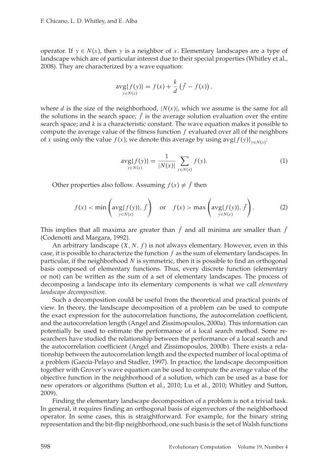
operator. If y ∈ N (x), then y is a neighbor of x. Elementary landscapes are a type oflandscape which are of particular interest due to their special properties (Whitley et al.,2008). They are characterized by a wave equation:
avg{f (y)}y∈N(x)
= f (x) + k
d
(f − f (x)
),
where d is the size of the neighborhood, |N (x)|, which we assume is the same for allthe solutions in the search space; f is the average solution evaluation over the entiresearch space; and k is a characteristic constant. The wave equation makes it possible tocompute the average value of the fitness function f evaluated over all of the neighborsof x using only the value f (x); we denote this average by using avg{f (y)}
y∈N(x):
avg{f (y)}y∈N(x)
= 1|N (x)|
∑y∈N(x)
f (y). (1)
Other properties also follow. Assuming f (x) �= f then
f (x) < min
(avg{f (y)}
y∈N(x), f
)or f (x) > max
(avg{f (y)}
y∈N(x), f
). (2)
This implies that all maxima are greater than f and all minima are smaller than f
(Codenotti and Margara, 1992).An arbitrary landscape (X,N, f ) is not always elementary. However, even in this
case, it is possible to characterize the function f as the sum of elementary landscapes. Inparticular, if the neighborhood N is symmetric, then it is possible to find an orthogonalbasis composed of elementary functions. Thus, every discrete function (elementaryor not) can be written as the sum of a set of elementary landscapes. The process ofdecomposing a landscape into its elementary components is what we call elementarylandscape decomposition.
Such a decomposition could be useful from the theoretical and practical points ofview. In theory, the landscape decomposition of a problem can be used to computethe exact expression for the autocorrelation functions, the autocorrelation coefficient,and the autocorrelation length (Angel and Zissimopoulos, 2000a). This information canpotentially be used to estimate the performance of a local search method. Some re-searchers have studied the relationship between the performance of a local search andthe autocorrelation coefficient (Angel and Zissimopoulos, 2000b). There exists a rela-tionship between the autocorrelation length and the expected number of local optima ofa problem (Garcıa-Pelayo and Stadler, 1997). In practice, the landscape decompositiontogether with Grover’s wave equation can be used to compute the average value of theobjective function in the neighborhood of a solution, which can be used as a base fornew operators or algorithms (Sutton et al., 2010; Lu et al., 2010; Whitley and Sutton,2009).
Finding the elementary landscape decomposition of a problem is not a trivial task.In general, it requires finding an orthogonal basis of eigenvectors of the neighborhoodoperator. In some cases, this is straightforward. For example, for the binary stringrepresentation and the bit-flip neighborhood, one such basis is the set of Walsh functions
598 Evolutionary Computation Volume 19, Number 4

Methodology to Find the Elementary Landscape Decomposition
(Sutton et al., 2009). Using the Walsh decomposition one can show that MAX k-SAT is asuperposition of k elementary landscapes, and every NK-landscape is a superpositionof K + 1 elementary landscapes. But for other representations, finding the orthogonalbasis of eigenvectors can be difficult (Angel and Zissimopoulos, 2000b).
This paper makes three fundamental contributions to research on elementary land-scapes. First, new theoretical results are presented that generalize our understanding ofelementary landscapes and their properties. Second, we develop a methodology basedon linear algebra that can potentially be used to find a decomposition of a function intoa linear combination of subfunctions, where each subfunction is elementary. Finally, wethen use this methodology to prove that the subset sum problem is a superposition oftwo elementary landscapes, and the quadratic assignment problem is a superpositionof three elementary landscapes. Showing that a problem is a superposition of elemen-tary landscapes makes it possible to extend many calculations which can be done onelementary landscapes (such as computing neighborhood averages and the exact au-tocorrelation of the neighborhood structure) to these other landscapes which are notdirectly elementary.
The organization of the paper is as follows. In Section 2 we first review elementarylandscapes, then present new theorems that provide the foundations needed to supportthe methods used later in this paper. Section 3 presents the proposed methodology andillustrates the explanations with a simple example, the subset sum problem. Section 4illustrates the methodology in a complex example, the quadratic assignment problem(QAP). In Section 5 we present some limitations of the proposed methodology and,finally, Section 6 concludes the paper and proposes some lines of future research.
2 Background and Theoretical Foundations
In this section we present some fundamental results on landscapes theory. Most ofthe results presented here can be found in previous work (Reidys and Stadler, 2002).However, we highlight some observations that can be easily derived from well-knownfacts but are not present in the previous literature as far as we know.
Let X be a finite set of solutions, f : X → R be a real-valued function defined onX, and N : X → P(X) the neighborhood operator. The pair (X,N ) is called configurationspace and can be represented using a graph G(X,E) in which X is the set of vertices anda directed edge (x, y) exists in E if y ∈ N (x) (Biyikoglu et al., 2007). We can representthe neighborhood operator by its adjacency matrix
Axy ={
1 if y ∈ N (x)0 otherwise . (3)
The degree matrix D is defined as the diagonal matrix
Dxy ={ |N (x)| if x = y
0 otherwise . (4)
Any discrete function, f , defined over the set of candidate solutions can be charac-terized as a vector in R
|X|. Using the graph representation of the configuration space,any function f can be interpreted as a labeling of the nodes in the graph, where thelabel of node x is f (x). Any |X| × |X| matrix can be interpreted as a linear map that acts
Evolutionary Computation Volume 19, Number 4 599
F. Chicano, L. D. Whitley, and E. Alba
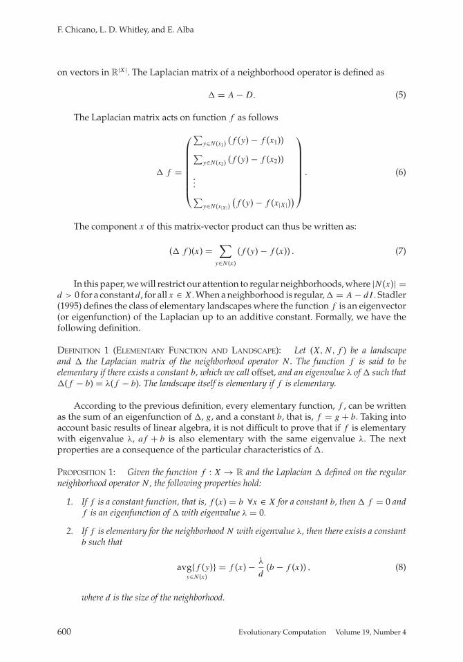
on vectors in R|X|. The Laplacian matrix of a neighborhood operator is defined as
� = A − D. (5)
The Laplacian matrix acts on function f as follows
� f =
⎛⎜⎜⎜⎜⎜⎜⎜⎝
∑y∈N(x1) (f (y) − f (x1))∑y∈N(x2) (f (y) − f (x2))
...∑y∈N(x|X|)
(f (y) − f (x|X|)
)
⎞⎟⎟⎟⎟⎟⎟⎟⎠
. (6)
The component x of this matrix-vector product can thus be written as:
(� f )(x) =∑
y∈N(x)
(f (y) − f (x)) . (7)
In this paper, we will restrict our attention to regular neighborhoods, where |N (x)| =d > 0 for a constant d, for all x ∈ X. When a neighborhood is regular, � = A − dI . Stadler(1995) defines the class of elementary landscapes where the function f is an eigenvector(or eigenfunction) of the Laplacian up to an additive constant. Formally, we have thefollowing definition.
DEFINITION 1 (ELEMENTARY FUNCTION AND LANDSCAPE): Let (X,N, f ) be a landscapeand � the Laplacian matrix of the neighborhood operator N . The function f is said to beelementary if there exists a constant b, which we call offset, and an eigenvalue λ of � such that�(f − b) = λ(f − b). The landscape itself is elementary if f is elementary.
According to the previous definition, every elementary function, f , can be writtenas the sum of an eigenfunction of �, g, and a constant b, that is, f = g + b. Taking intoaccount basic results of linear algebra, it is not difficult to prove that if f is elementarywith eigenvalue λ, af + b is also elementary with the same eigenvalue λ. The nextproperties are a consequence of the particular characteristics of �.
PROPOSITION 1: Given the function f : X → R and the Laplacian � defined on the regularneighborhood operator N , the following properties hold:
1. If f is a constant function, that is, f (x) = b ∀x ∈ X for a constant b, then � f = 0 andf is an eigenfunction of � with eigenvalue λ = 0.
2. If f is elementary for the neighborhood N with eigenvalue λ, then there exists a constantb such that
avg{f (y)}y∈N(x)
= f (x) − λ
d(b − f (x)) , (8)
where d is the size of the neighborhood.
600 Evolutionary Computation Volume 19, Number 4

Methodology to Find the Elementary Landscape Decomposition
PROOF: For the first property we can use Equation (7) and write:
(� f )(x) =∑
y∈N(x)
(f (y) − f (x)) =∑
y∈N(x)
(b − b) = 0.
This happens for each x ∈ X, so �f = 0 and it is an eigenfunction of � with eigen-value 0.
For the second property we again use Equation (7) to write:
(�f )(x) =∑
y∈N(x)
(f (y) − f (x)) =∑
y∈N(x)
f (y) − d f (x).
Dividing by d the previous equation we get:
1d
(�f )(x) = avg{f (y)}y∈N(x)
−f (x). (9)
Since f is elementary with eigenvalue λ, there exists a constant b such that �(f −b) = λ(f − b). Then, we can write the following with the help of Equation (9):
1d
(�(f − b))(x) = 1d
(�f )(x) = avg{f (y)}y∈N(x)
−f (x) = λ
d(f (x) − b),
where we used the first property to remove b from the first member. We can rewrite thelast two members as
avg{f (y)}y∈N(x)
= f (x) − λ
d(b − f (x)).
�
What is generally known as Grover’s wave equation is just a particular instance ofthis more general result, for which Grover’s equation b = f , where is f the average ofthe function f over the entire solution set X, that is, f = (∑
x∈X f (x))/|X|. As far as we
know, Equation (8) has not previously been reported in the literature. Its relevance comesfrom the fact that it is valid in all the regular neighborhoods (not only in the symmetricones). Grover’s wave equation can be stated as a special case of Proposition 1 in whichthe neighborhood is symmetric.
THEOREM 1 (GROVER’S WAVE EQUATION): The landscape (X,N, f ) with N symmetric andregular is elementary if and only if the following expression holds:
avg{f (y)}y∈N(x)
= f (x) + k
d
(f − f (x)
) ∀x ∈ X, (10)
where k is the additive inverse of the eigenvalue of f , that is, k = −λ.
Evolutionary Computation Volume 19, Number 4 601

F. Chicano, L. D. Whitley, and E. Alba
Grover’s equation requires that the neighborhood be symmetric and regular. Wesay that a neighborhood N is symmetric if for all x, y ∈ X it holds that y ∈ N (x) impliesx ∈ N (y), that is, if y is a neighbor of x then x is a neighbor of y.
In Proposition 1 we proved that constant functions are eigenvectors of � withλ = 0. Now we can ask the opposite: are all the eigenvectors of � with λ = 0 constantfunctions? The general answer is no. However, as it is stated by Stadler (1996), if theneighborhood N is connected then the multiplicity of the eigenvalue λ = 0 is one, andthis means that only constant functions are eigenvectors of �. Thus, for connectedneighborhoods the answer to the previous question is yes. We say that a neighborhoodN is connected if for each pair of solutions x, y ∈ X we can find a finite sequence ofsolutions x = x1, x2, . . . , xq = y such that xi+1 ∈ N (xi) for i = 1, 2, . . . , q − 1.
From Grover’s wave equation we conclude that in an elementary landscape thereexists a linear relationship between the average of the function in the neighborhood ofa solution and the value of the function in that solution. We now ask if the linear rela-tionship is a general characteristic of elementary landscapes. The following propositionpositively answers this question.
PROPOSITION 2: Let (X,N, f ) be a landscape where the neighborhood, N , is regular andsymmetric. Then, f is elementary if and only if there exist two constants α and β such that:
avg{f (y)}y∈N(x)
= αf (x) + β ∀x ∈ X. (11)
PROOF: If the landscape is elementary, then Equation (11) follows from Theorem 1.Let us prove the reciprocal implication. We assume that Equation (11) holds. Then, wecan multiply both members by d to write:
∑y∈N(x)
f (y) = dαf (x) + dβ = df (x) + d (α − 1)f (x) + dβ.
If we subtract d f (x) we have:
∑y∈N(x)
f (y) − d f (x) = d (α − 1)f (x) + dβ.
At this point we must consider two cases. First, let us consider the case in which α = 1,then we can write the previous equation in vector form as:
�f = dβ
⎛⎜⎜⎜⎜⎜⎜⎝
1
1
...
1
⎞⎟⎟⎟⎟⎟⎟⎠
.
602 Evolutionary Computation Volume 19, Number 4
Methodology to Find the Elementary Landscape Decomposition
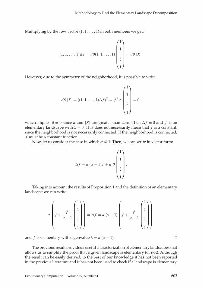
Multiplying by the row vector (1, 1, . . . , 1) in both members we get:
(1, 1, . . . , 1)�f = dβ(1, 1, . . . , 1)
⎛⎜⎜⎜⎜⎜⎜⎝
1
1
...
1
⎞⎟⎟⎟⎟⎟⎟⎠
= dβ |X|.
However, due to the symmetry of the neighborhood, it is possible to write:
dβ |X| = ((1, 1, . . . , 1)�f )T = f T �
⎛⎜⎜⎜⎜⎜⎜⎝
1
1
...
1
⎞⎟⎟⎟⎟⎟⎟⎠
= 0,
which implies β = 0 since d and |X| are greater than zero. Then �f = 0 and f is anelementary landscape with λ = 0. This does not necessarily mean that f is a constant,since the neighborhood is not necessarily connected. If the neighborhood is connected,f must be a constant function.
Now, let us consider the case in which α �= 1. Then, we can write in vector form:
�f = d (α − 1)f + d β
⎛⎜⎜⎜⎜⎜⎜⎝
1
1
...
1
⎞⎟⎟⎟⎟⎟⎟⎠
.
Taking into account the results of Proposition 1 and the definition of an elementarylandscape we can write:
�
⎛⎜⎜⎜⎜⎜⎜⎝
f + β
α − 1
⎛⎜⎜⎜⎜⎜⎜⎝
1
1
...
1
⎞⎟⎟⎟⎟⎟⎟⎠
⎞⎟⎟⎟⎟⎟⎟⎠
= �f = d (α − 1)
⎛⎜⎜⎜⎜⎜⎜⎝
f + β
α − 1
⎛⎜⎜⎜⎜⎜⎜⎝
1
1
...
1
⎞⎟⎟⎟⎟⎟⎟⎠
⎞⎟⎟⎟⎟⎟⎟⎠
,
and f is elementary with eigenvalue λ = d (α − 1). �
The previous result provides a useful characterization of elementary landscapes thatallows us to simplify the proof that a given landscape is elementary (or not). Althoughthe result can be easily derived, to the best of our knowledge it has not been reportedin the previous literature and it has not been used to check if a landscape is elementary.
Evolutionary Computation Volume 19, Number 4 603

F. Chicano, L. D. Whitley, and E. Alba
When f is not an elementary landscape, Equation (11) does not hold, but we can find ageneralization of the equation that does hold if f is the sum of n elementary landscapes.This general expression is presented in the following.
THEOREM 2: Let (X,N, f ) be a landscape in which the neighborhood, N , is regular andsymmetric. Then, f is the sum of n nonconstant elementary landscapes fi if and only if thereexist some constants αi for i = 0, 1, . . . , n such that
avg{f (y)}y∈N(x)
= α0 + α1f (x) +n∑
i=2
αifi(x) ∀x ∈ X. (12)
PROOF: We can prove this by induction on n. In the base case, n = 1, Proposition 2holds and the statement is true. For the inductive step, let us assume that the statementis true for n − 1 and let us prove the result for n.
Assume the function f is the sum of n elementary landscapes fi , that is:
f =n∑
i=1
fi.
If we subtract fn in the previous equality, then f − fn is the sum of n − 1 elementarylandscapes. We can apply the inductive hypothesis to compute the average value in theneighborhood of an arbitrary solution x. That is, a set of constants αi exists such that:
avg{f (y) − fn(y)}y∈N(x)
= α0 + α1(f (x) − fn(x)) +n−1∑i=2
αifi(x). (13)
Since fn is an elementary landscape, according to Proposition 2 we can writeavg{fn(y)}
y∈N(x) = β0 + β1fn(x), and the previous expression can be written as:
avg{f (y)}y∈N(x)
= α0 + α1(f (x) − fn(x)) +n−1∑i=2
αifi(x) + avg{fn(y)}y∈N(x)
= α0 + α1(f (x) − fn(x)) +n−1∑i=2
αifi(x) + β0 + β1fn(x)
= (α0 + β0) + α1f (x) +n−1∑i=2
αifi(x) + (β1 − α1)fn(x)
and Equation (12) holds for n.Let us now prove the reciprocal implication. Let us assume that Equation (12) holds
for a given f , where all fi are elementary functions. Since fn is a nonconstant elementaryfunction, we can apply Proposition 2 and write avg{fn(y)}
y∈N(x) = β0 + β1fn(x) with
604 Evolutionary Computation Volume 19, Number 4
Methodology to Find the Elementary Landscape Decomposition
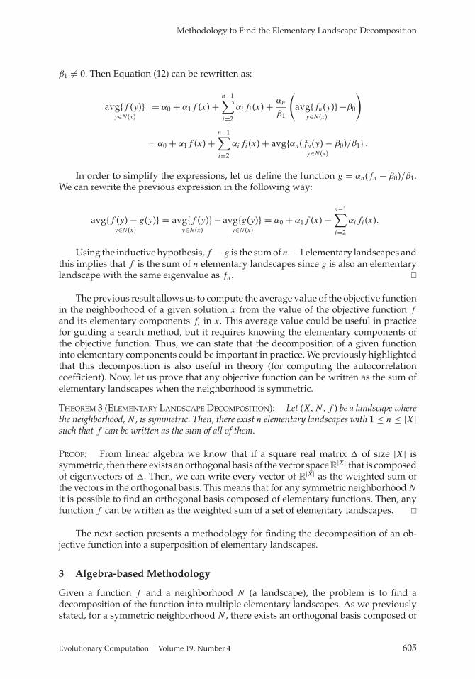
β1 �= 0. Then Equation (12) can be rewritten as:
avg{f (y)}y∈N(x)
= α0 + α1f (x) +n−1∑i=2
αifi(x) + αn
β1
(avg{fn(y)}
y∈N(x)−β0
)
= α0 + α1f (x) +n−1∑i=2
αifi(x) + avg{αn(fn(y) − β0)/β1}y∈N(x)
.
In order to simplify the expressions, let us define the function g = αn(fn − β0)/β1.We can rewrite the previous expression in the following way:
avg{f (y) − g(y)}y∈N(x)
= avg{f (y)}y∈N(x)
− avg{g(y)}y∈N(x)
= α0 + α1f (x) +n−1∑i=2
αifi(x).
Using the inductive hypothesis, f − g is the sum of n − 1 elementary landscapes andthis implies that f is the sum of n elementary landscapes since g is also an elementarylandscape with the same eigenvalue as fn. �
The previous result allows us to compute the average value of the objective functionin the neighborhood of a given solution x from the value of the objective function f
and its elementary components fi in x. This average value could be useful in practicefor guiding a search method, but it requires knowing the elementary components ofthe objective function. Thus, we can state that the decomposition of a given functioninto elementary components could be important in practice. We previously highlightedthat this decomposition is also useful in theory (for computing the autocorrelationcoefficient). Now, let us prove that any objective function can be written as the sum ofelementary landscapes when the neighborhood is symmetric.
THEOREM 3 (ELEMENTARY LANDSCAPE DECOMPOSITION): Let (X,N, f ) be a landscape wherethe neighborhood, N , is symmetric. Then, there exist n elementary landscapes with 1 ≤ n ≤ |X|such that f can be written as the sum of all of them.
PROOF: From linear algebra we know that if a square real matrix � of size |X| issymmetric, then there exists an orthogonal basis of the vector space R
|X| that is composedof eigenvectors of �. Then, we can write every vector of R
|X| as the weighted sum ofthe vectors in the orthogonal basis. This means that for any symmetric neighborhood N
it is possible to find an orthogonal basis composed of elementary functions. Then, anyfunction f can be written as the weighted sum of a set of elementary landscapes. �
The next section presents a methodology for finding the decomposition of an ob-jective function into a superposition of elementary landscapes.
3 Algebra-based Methodology
Given a function f and a neighborhood N (a landscape), the problem is to find adecomposition of the function into multiple elementary landscapes. As we previouslystated, for a symmetric neighborhood N , there exists an orthogonal basis composed of
Evolutionary Computation Volume 19, Number 4 605
F. Chicano, L. D. Whitley, and E. Alba
elementary landscapes. Let us denote this basis with θλ,i where λ is the eigenvalue ofthe vector (function) and i is an index to distinguish the different vectors with the sameeigenvalue. Then a Fourier expansion of f is
f =∑
λ
∑i
aλ,iθλ,i ,
where the values aλ,i = ⟨θλ,i , f
⟩are the Fourier coefficients. Using this Fourier expansion,
it is possible to compute the landscape decomposition by summing the terms with thesame eigenvalue. Each elementary component can be computed as
fλ =∑
i
aλ,iθλ,i . (14)
A special case is that of f0, the elementary landscape with λ = 0. We assume that theneighborhood is connected. Then, f0 is the constant value f , and it could be added to anyof the other elementary components and still the landscape would remain elementary.
Equation (14) can be used when an orthogonal basis of eigenvectors is known forthe neighborhood. This happens, for example, in the case of binary strings with thebit-flip neighborhood. An appropriate basis for this neighborhood is the set of Walshfunctions (Sutton et al., 2009). But in general such a basis is not known or, when it isknown, it is not easy to compute the Fourier coefficients. The methodology we presenthere is useful under these situations.
The methodology consists of analyzing instances of the problem that are smallenough that it is possible to enumerate the Laplacian matrix �. This way, it is possibleto obtain a basis of R
|X| composed of eigenvectors of �. With the help of this basis wecan decompose the objective function into subfunctions which are elementary. Then, adetailed study of the elementary components can reveal the general definition of thesecomponents in any general (and larger) instance of the problem.
We have identified five steps for applying the methodology:
1. Rewrite the objective function as a linear combination of the so-called basic func-tions, denoted with ϕ.
2. Compute � and ϕ for small instances.
3. Compute the projections of ϕ in the eigenspaces of �.
4. Analyze the projections and propose elementary components.
5. Check the landscape decomposition in the general case.
In the following we explain in detail the operations involved in each step and we il-lustrate the application of this methodology with a landscape decomposition for the sub-set sum problem (Garey and Johnson, 1979). Given a set of integers S = {s1, s2, . . . , sn},the problem consists of finding a nonempty subset of S whose sum is C (if any). Thisproblem can be transformed as a minimization problem with objective function
f (x) =(
n∑i=1
sixi − C
)2
, (15)
606 Evolutionary Computation Volume 19, Number 4

Methodology to Find the Elementary Landscape Decomposition
where xi ∈ {0, 1} are the decision variables of the problem. Thus, the size of the solutionspace X is 2n, and the neighborhood is the bit-flip neighborhood: two solutions areneighbors if one of them can be obtained by changing the value of one decision variablexi in the other one.
3.1 Step 1: Rewrite the Objective Function
In order to analyze the elementary components of the objective function, it is usefulto separate the definition of the objective function into (1) the information that is par-ticular to a given instance (the data of the instance); and (2) the general relationshipsthat characterize the class of the problem. We are interested in linear combinations offunctions, called basic functions, where the coefficients of the functions are the data ofthe particular instances. Note that any linear combination of elementary functions withthe same characteristic constant k is also an elementary function. Then we reduce theanalysis of the general objective function containing instance information to the analysisof a family of basic functions that do not depend on the instance data. We denote thesebasic functions with the letter ϕ and we use subscripts and superscripts to parameterizethe basic functions.
We illustrate this first step using the subset sum problem. We can rewrite Equation(15) in the following way:
f (x) =(
n∑i=1
sixi − C
)2
=n∑
i,j=1
sisj xixj − 2C
n∑i=1
sixi + C2
=n∑
i,j=1
sisjϕij (x) − 2C
n∑i=1
siϕii(x) + C2 (16)
where we write f as a linear combination of the parameterized functions ϕij (x) = xixj .All the information related to each particular instance is focused on the weights (thecoefficients) of this linear combination. Thus, we only have to study the family of basicfunctions ϕij . Using the landscape decomposition of these basic functions, it is possibleto compute the landscape decomposition of f for any instance of the problem (set S).
3.2 Step 2: Compute � and ϕ for Small Instances
Recall that we are dealing with a problem class. This means that we are analyzing a(possibly infinite) set of problem instances at the same time. These instances can havedifferent sizes, and by size we mean the cardinality of the solution space X. For example,in the subset sum problem we have
|X| = 2n
where n is the number of integers in the set S.In the second step of this methodology we need to explicitly compute the Laplacian
matrix � and we explicitly represent the basic functions ϕ using a vector. Thus, thelarger the cardinality of X, the larger the size of � and ϕ. Since we have to numericallyoperate with � and ϕ, it is preferable to work with small solution spaces. The numberof solution spaces required depends on the number of elementary components of ϕ. Agood rule of thumb here is to use the smaller solution spaces for which the Laplacianmatrix has a size that affords its use with a computer algebra system.
Evolutionary Computation Volume 19, Number 4 607
F. Chicano, L. D. Whitley, and E. Alba
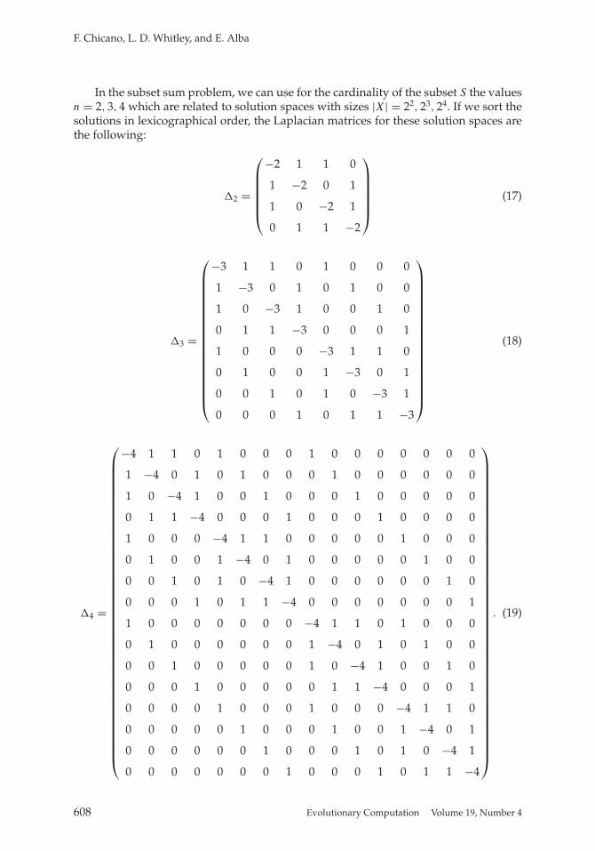
In the subset sum problem, we can use for the cardinality of the subset S the valuesn = 2, 3, 4 which are related to solution spaces with sizes |X| = 22, 23, 24. If we sort thesolutions in lexicographical order, the Laplacian matrices for these solution spaces arethe following:
�2 =
⎛⎜⎜⎜⎜⎜⎝
−2 1 1 0
1 −2 0 1
1 0 −2 1
0 1 1 −2
⎞⎟⎟⎟⎟⎟⎠ (17)
�3 =
⎛⎜⎜⎜⎜⎜⎜⎜⎜⎜⎜⎜⎜⎜⎜⎜⎜⎜⎝
−3 1 1 0 1 0 0 0
1 −3 0 1 0 1 0 0
1 0 −3 1 0 0 1 0
0 1 1 −3 0 0 0 1
1 0 0 0 −3 1 1 0
0 1 0 0 1 −3 0 1
0 0 1 0 1 0 −3 1
0 0 0 1 0 1 1 −3
⎞⎟⎟⎟⎟⎟⎟⎟⎟⎟⎟⎟⎟⎟⎟⎟⎟⎟⎠
(18)
�4 =
⎛⎜⎜⎜⎜⎜⎜⎜⎜⎜⎜⎜⎜⎜⎜⎜⎜⎜⎜⎜⎜⎜⎜⎜⎜⎜⎜⎜⎜⎜⎜⎜⎜⎜⎜⎜⎜⎜⎜⎜⎜⎜⎝
−4 1 1 0 1 0 0 0 1 0 0 0 0 0 0 0
1 −4 0 1 0 1 0 0 0 1 0 0 0 0 0 0
1 0 −4 1 0 0 1 0 0 0 1 0 0 0 0 0
0 1 1 −4 0 0 0 1 0 0 0 1 0 0 0 0
1 0 0 0 −4 1 1 0 0 0 0 0 1 0 0 0
0 1 0 0 1 −4 0 1 0 0 0 0 0 1 0 0
0 0 1 0 1 0 −4 1 0 0 0 0 0 0 1 0
0 0 0 1 0 1 1 −4 0 0 0 0 0 0 0 1
1 0 0 0 0 0 0 0 −4 1 1 0 1 0 0 0
0 1 0 0 0 0 0 0 1 −4 0 1 0 1 0 0
0 0 1 0 0 0 0 0 1 0 −4 1 0 0 1 0
0 0 0 1 0 0 0 0 0 1 1 −4 0 0 0 1
0 0 0 0 1 0 0 0 1 0 0 0 −4 1 1 0
0 0 0 0 0 1 0 0 0 1 0 0 1 −4 0 1
0 0 0 0 0 0 1 0 0 0 1 0 1 0 −4 1
0 0 0 0 0 0 0 1 0 0 0 1 0 1 1 −4
⎞⎟⎟⎟⎟⎟⎟⎟⎟⎟⎟⎟⎟⎟⎟⎟⎟⎟⎟⎟⎟⎟⎟⎟⎟⎟⎟⎟⎟⎟⎟⎟⎟⎟⎟⎟⎟⎟⎟⎟⎟⎟⎠
. (19)
608 Evolutionary Computation Volume 19, Number 4

Methodology to Find the Elementary Landscape Decomposition
Now we need a vector representation of the basic functions. Usually not all thebasic functions are needed, since some of them are equivalent. We say that two basicfunctions ϕ and ϕ′ are equivalent if there exists an automorphism π : X → X of thegraph G induced by the configuration space such that ϕ ◦ π = ϕ′. In other words, wesay that two basic functions are equivalent if they are essentially the same function seenfrom a different point of view of the graph. We can partition the family of basic functionsaccording to the previous equivalence relation and study only one basic function fromeach equivalence class.
In the subset sum problem, the basic functions ϕij can be partitioned into twoequivalence classes: those in which i �= j and those for which i = j . In effect, for a pairof basic functions ϕij and ϕi ′j ′ in which i �= j and i ′ �= j ′ an automorphism for whichϕi ′j ′ ◦ π = ϕij is:
π : X → X
π (x) �→ y
where yi = xi ′ , yi ′ = xi , yj = xj ′, yj ′ = xj and yk = xk for k �= i, i ′, j, j ′. For a pair of basicfunctions ϕii and ϕi ′i ′ an automorphism for which ϕi ′i ′ ◦ π = ϕii is π where π (x) = y
and yi = xi′, yi ′ = xi , and yk = xk for k �= i, i ′. On the other hand, the basic functionsϕii and ϕij cannot be equivalent if j �= i since both functions have a different numberof solutions with value 1. Having the same number of solutions with a given functionvalue is a necessary condition for equivalence.
As a sample of the two equivalence classes in which the basic functions can bepartitioned, let us study the functions ϕ12 and ϕ11 for the cardinalities of S used beforen = 2, 3, 4. In vector form these basic functions are:
�ϕ11 = (0 1 0 1
)T
�ϕ12 = (0 0 0 1
)T for n = 2 (20)
�ϕ11 = (0 1 0 1 0 1 0 1
)T
�ϕ12 = (0 0 0 1 0 0 0 1
)T for n = 3 (21)
�ϕ11 = (0 1 0 1 0 1 0 1 0 1 0 1 0 1 0 1
)T
�ϕ12 = (0 0 0 1 0 0 0 1 0 0 0 1 0 0 0 1
)T for n = 4. (22)
We use the two notations ϕ and �ϕ (with the corresponding subscripts and super-scripts) to represent the basic functions. However, we use vector notation when wewant to highlight the vector nature of the function.
3.3 Step 3: Compute the Projections of ϕ in the Eigenspaces of �
In this step we decompose the basic functions into their elementary components for theinstance sizes considered in the previous step. In order to do this, we first compute theeigenvalues of the Laplacian and an orthonormal vector basis composed of eigenvectors,
Evolutionary Computation Volume 19, Number 4 609
F. Chicano, L. D. Whitley, and E. Alba
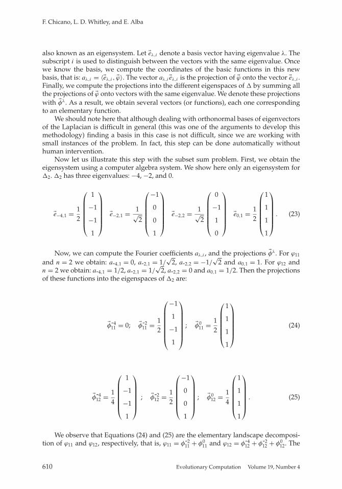
also known as an eigensystem. Let �eλ,i denote a basis vector having eigenvalue λ. Thesubscript i is used to distinguish between the vectors with the same eigenvalue. Oncewe know the basis, we compute the coordinates of the basic functions in this newbasis, that is: aλ,i = 〈�eλ,i , �ϕ〉. The vector aλ,i�eλ,i is the projection of �ϕ onto the vector �eλ,i .Finally, we compute the projections into the different eigenspaces of � by summing allthe projections of �ϕ onto vectors with the same eigenvalue. We denote these projectionswith �φλ. As a result, we obtain several vectors (or functions), each one correspondingto an elementary function.
We should note here that although dealing with orthonormal bases of eigenvectorsof the Laplacian is difficult in general (this was one of the arguments to develop thismethodology) finding a basis in this case is not difficult, since we are working withsmall instances of the problem. In fact, this step can be done automatically withouthuman intervention.
Now let us illustrate this step with the subset sum problem. First, we obtain theeigensystem using a computer algebra system. We show here only an eigensystem for�2. �2 has three eigenvalues: −4, −2, and 0.
�e−4,1 = 12
⎛⎜⎜⎜⎜⎜⎝
1
−1
−1
1
⎞⎟⎟⎟⎟⎟⎠ �e−2,1 = 1√
2
⎛⎜⎜⎜⎜⎜⎝
−1
0
0
1
⎞⎟⎟⎟⎟⎟⎠ �e−2,2 = 1√
2
⎛⎜⎜⎜⎜⎜⎝
0
−1
1
0
⎞⎟⎟⎟⎟⎟⎠ �e0,1 = 1
2
⎛⎜⎜⎜⎜⎜⎝
1
1
1
1
⎞⎟⎟⎟⎟⎟⎠ . (23)
Now, we can compute the Fourier coefficients aλ,i , and the projections �φλ. For ϕ11
and n = 2 we obtain: a-4,1 = 0, a-2,1 = 1/√
2, a-2,2 = −1/√
2 and a0,1 = 1. For ϕ12 andn = 2 we obtain: a-4,1 = 1/2, a-2,1 = 1/
√2, a-2,2 = 0 and a0,1 = 1/2. Then the projections
of these functions into the eigenspaces of �2 are:
�φ-411 = 0; �φ-2
11 = 12
⎛⎜⎜⎜⎜⎜⎜⎝
−1
1
−1
1
⎞⎟⎟⎟⎟⎟⎟⎠
; �φ011 = 1
2
⎛⎜⎜⎜⎜⎜⎝
1
1
1
1
⎞⎟⎟⎟⎟⎟⎠ (24)
�φ-412 = 1
4
⎛⎜⎜⎜⎜⎜⎝
1
−1
−1
1
⎞⎟⎟⎟⎟⎟⎠ ; �φ-2
12 = 12
⎛⎜⎜⎜⎜⎜⎝
−1
0
0
1
⎞⎟⎟⎟⎟⎟⎠ ; �φ0
12 = 14
⎛⎜⎜⎜⎜⎜⎝
1
1
1
1
⎞⎟⎟⎟⎟⎟⎠ . (25)
We observe that Equations (24) and (25) are the elementary landscape decomposi-tion of ϕ11 and ϕ12, respectively, that is, ϕ11 = φ-2
11 + φ011 and ϕ12 = φ-4
12 + φ-212 + φ0
12. The
610 Evolutionary Computation Volume 19, Number 4
Methodology to Find the Elementary Landscape Decomposition
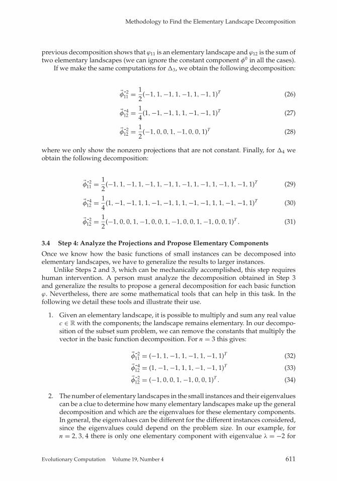
previous decomposition shows that ϕ11 is an elementary landscape and ϕ12 is the sum oftwo elementary landscapes (we can ignore the constant component φ0 in all the cases).
If we make the same computations for �3, we obtain the following decomposition:
�φ-211 = 1
2(−1, 1,−1, 1,−1, 1,−1, 1)T (26)
�φ-412 = 1
4(1,−1,−1, 1, 1,−1,−1, 1)T (27)
�φ-212 = 1
2(−1, 0, 0, 1,−1, 0, 0, 1)T (28)
where we only show the nonzero projections that are not constant. Finally, for �4 weobtain the following decomposition:
�φ-211 = 1
2(−1, 1,−1, 1,−1, 1,−1, 1,−1, 1,−1, 1,−1, 1,−1, 1)T (29)
�φ-412 = 1
4(1,−1,−1, 1, 1,−1,−1, 1, 1,−1,−1, 1, 1,−1,−1, 1)T (30)
�φ-212 = 1
2(−1, 0, 0, 1,−1, 0, 0, 1,−1, 0, 0, 1,−1, 0, 0, 1)T . (31)
3.4 Step 4: Analyze the Projections and Propose Elementary Components
Once we know how the basic functions of small instances can be decomposed intoelementary landscapes, we have to generalize the results to larger instances.
Unlike Steps 2 and 3, which can be mechanically accomplished, this step requireshuman intervention. A person must analyze the decomposition obtained in Step 3and generalize the results to propose a general decomposition for each basic functionϕ. Nevertheless, there are some mathematical tools that can help in this task. In thefollowing we detail these tools and illustrate their use.
1. Given an elementary landscape, it is possible to multiply and sum any real valuec ∈ R with the components; the landscape remains elementary. In our decompo-sition of the subset sum problem, we can remove the constants that multiply thevector in the basic function decomposition. For n = 3 this gives:
�φ-211 = (−1, 1,−1, 1,−1, 1,−1, 1)T (32)
�φ-412 = (1,−1,−1, 1, 1,−1,−1, 1)T (33)
�φ-212 = (−1, 0, 0, 1,−1, 0, 0, 1)T . (34)
2. The number of elementary landscapes in the small instances and their eigenvaluescan be a clue to determine how many elementary landscapes make up the generaldecomposition and which are the eigenvalues for these elementary components.In general, the eigenvalues can be different for the different instances considered,since the eigenvalues could depend on the problem size. In our example, forn = 2, 3, 4 there is only one elementary component with eigenvalue λ = −2 for
Evolutionary Computation Volume 19, Number 4 611

F. Chicano, L. D. Whitley, and E. Alba
Figure 1: Graph G = (X,E) for n = 2. We label the nodes with φ(x)x . The equivalenceclass [00] contains 00 and 10 which both have evaluation –1.
ϕ11 and two elementary components for ϕ12 with eigenvalues λ = −2,−4. Thus,we conjecture that in the general case, ϕ11 is an elementary component and ϕ12can be decomposed as two elementary components with eigenvalues λ = −2 andλ = −4, respectively.
3. We can use the underlying graph of the landscape G = (X,E) as a tool in theanalysis of the landscape decomposition. To this aim we need to label the nodesof the graph with the values of the function φ. Then, we construct a new graphby grouping together all the nodes that we consider equivalent according to thefunction value and graph structure. Equivalent now means not only to have thesame function value, but their neighbors must also be equivalent. In formal terms,we say that two nodes x and y in the graph are equivalent for function φ, andwe denote it with x ∼φ y when there exists an automorphism π of the graphsuch that π (x) = y and φ ◦ π = φ. That is, in a graph labeled with function φ, thenodes x and y cannot be distinguished. With this equivalence relationship thenew graph is G/ ∼φ= (X/ ∼φ, E/ ∼φ) where X/ ∼φ is the quotient set of X by ∼φ
and ([x], [y]) ∈ E/ ∼φ if (x, y) ∈ E. The set X/ ∼φ is the set of equivalence classesin set X, and we use [x] to denote the equivalence class containing x. In G/ ∼φ
we label each node [x] with the value φ(x). In addition, for this graph we alsolabel each edge ([x], [y]) with the number of edges in the original graph G of theform (x, z) where z ∈ [y]. In other words, the label of ([x], [y]) is the number ofneighbors that any element in [x] has with function value φ(y). This graph mustbe constructed for each elementary component φ of each basic function ϕ in allthe small instances considered. In the following we call this graph the reducedgraph for function φ.
Let us illustrate the graph construction with φ-211 for n = 2. The original labeled
graph is the one shown in Figure 1, where we also show the solution x with thefunction value φ(x). It is not difficult to see in this case that nodes 00 and 10 areequivalent and the same is true for 01 and 11. Then the reduced graph G/ ∼φ-2
11is
the one shown in Figure 2.We have computed the reduced graph for all the φ functions and we show
them in Figures 3, 4, and 5.
The reduced graphs can help in identifying features of the elementary compo-nents in order to generalize their definition. In order to define the general elementary
612 Evolutionary Computation Volume 19, Number 4

Methodology to Find the Elementary Landscape Decomposition
Figure 2: Graph G/ ∼φ-211
for n = 2. We label the nodes with φ([x])[x].
Figure 3: Graph G/ ∼φ-211
for n = 2, 3, 4. We label the nodes with φ([x])[x].
Figure 4: Graph G/ ∼φ-212
for n = 2, 3, 4. We label the nodes with φ([x])[x].
components φ we first need to recognize this elementary component among the φ
functions of the small instances considered with different sizes. This can be done bygrouping together the φ functions of the different instances with some common feature.Then, we conjecture that these functions can be generalized to a most general elementary
Evolutionary Computation Volume 19, Number 4 613

F. Chicano, L. D. Whitley, and E. Alba
Figure 5: Graph G/ ∼φ-412
for n = 2, 3, 4. We label the nodes with φ([x])[x].
Table 1: Equivalence classes for the subset sum problem with function φ-212.
n = 2 n = 3 n = 4
[00] [01] [11] [000] [001] [011] [0000] [0001] [0011]
00 01 11 000 001 011 0000 0001 001110 100 010 111 0100 0010 0111
101 1000 0101 1011110 1100 0110 1111
1001101011011110
component. After that, we propose the generalization by observing the classes of equiv-alence in X/ ∼φ . Let us illustrate this with our example.
In Figures 3, 4, and 5 we have grouped together the φ functions according to theireigenvalues. As we previously argued, in this example it seems that ϕ11 is elementaryand ϕ12 can be decomposed into two elementary components with eigenvalues λ = −2and λ = −4. Then, it is reasonable to think that the functions φ-2
11 for the different valuesof n are elementary, and the same holds for φ-2
12 and φ-412. In this case, the grouping seems
evident. If the eigenvalues were different for the different sizes of the problem, then thegrouping would not be so evident.
The next step is, then, to propose a generalization for the grouped functions. Thesimplest case is that of φ-2
11, since its elementariness implies the elementariness of ϕ11,so we should be able to write φ-2
ii as a function of ϕii . A possible generalization of thisfunction is φ-2
ii = 2ϕii − 1 = 2xi − 1. In the fifth step we will check if this function iselementary or not.
Let us follow with φ-212. In Figure 4 we have not shown the equivalence classes. They
are shown in Table 1. In the table we show the values of xi in big-endian order (xn firstand x1 last). A closer look to the equivalence classes suggests that φ-2
12 = −1 if x1 = x2 = 0,φ-2
12 = 1 if x1 = x2 = 1, and φ-212 = 0 if x1 �= x2. Then, the proposed generalization is the
following:
φ-2ij =
⎧⎪⎨⎪⎩
−1 if xi = xj = 0
1 if xi = xj = 1.
0 if xi �= xj
(35)
614 Evolutionary Computation Volume 19, Number 4

Methodology to Find the Elementary Landscape Decomposition
Table 2: Equivalence classes for the subset sum problem with function φ-412.
n = 2 n = 3 n = 4
[00] [01] [000] [001] [0000] [0001]
00 01 000 001 0000 000111 10 011 010 0011 0010
100 101 0100 0101111 110 0111 0110
1000 10011011 10101100 11011111 1110
Let us now analyze φ-412 (Figure 5). In Table 2 we show the equivalence classes for
this function. The analysis suggests that φ-412 = 1 if x1 = x2 and φ-4
12 = −1 if x1 �= x2. Theproposed generalization is the following:
φ-4ij =
{1 if xi = xj
−1 if xi �= xj
. (36)
The final proposal of this step can be summarized as follows:
1. The function ϕii is an elementary landscape with λ = −2
2. The function ϕij with i �= j is the weighted sum of two elementary landscapes de-fined in Equations (35) and (36) with eigenvalues λ = −2 and λ = −4, respectively(up to an additive constant).
In the next, and final step, we check the proposal.
3.5 Step 5: Check the Landscape Decomposition in the General Case
In this final step we check the functions proposed in the previous step as elementarycomponents of the basic functions. The check consists in a formal proof of the ele-mentariness of the proposed functions or a counterexample showing that they are notelementary. In the case of the formal proof, a relevant result that can be useful is that ofProposition 2. If all the proposed functions are elementary, then we need a final checkto complete the landscape decomposition. We need to prove that the weighted sum ofthe elementary components is the actual basic function. If any of the checks fail, thenwe can go to Step 4 and try a different proposal.
The reader should note that the previous four steps were required to provide anelementary decomposition proposal for the problem at hand. But we have no proof upto the moment that the decomposition is correct for an arbitrary instance of the problem.In this step, we provide this proof. It is also important to highlight that even though theelementary functions proposed in Step 4 were a result of an inductive reasoning oversome small instances of the problem, the result we get in this fifth step is completelygeneral, and can be applied to any instance of any size of the problem. Thus, we shouldend the fifth step (and the methodology) with a theorem and the proof of that theoremis the operations we do to check the decomposition.
Evolutionary Computation Volume 19, Number 4 615

F. Chicano, L. D. Whitley, and E. Alba
Figure 6: Graphs G/ ∼φ-2ii
, G/ ∼φ-2ij
, and G/ ∼φ-4ij
.
Let us focus on our example. We start by showing that φ-2ii , φ-2
ij , and φ-4ij are elemen-
tary landscapes with the help of Proposition 2. We will again use the reduced graphsG/ ∼φ . However, instead of using the graphs for the particular instances n = 2, 3, 4, weuse a graph for the general function (arbitrary n). The general graphs for φ-2
ii , φ-2ij and
φ-4ij are shown in Figure 6. We can observe that the graphs in Figures 3, 4, and 5 are
particular cases of the ones in Figure 6.Let us prove that the graphs of Figure 6 are the reduced graphs for the corresponding
functions. In these graphs, the set of solutions are indicated as predicates in the nodes(the predicates used in the branches of the functions). We must take into account that,by the definition of reduced graph, two nodes of the original graph are in the sameequivalence class (node in the reduced graph) if (1) they have the same function value;and (2) all their neighbors are equivalent. In the graphs of Figure 6, all the solutionsin each node have the same function value, since the nodes have been defined afterthe predicates in the branches of the function definition. Then, the first condition issatisfied. In order to check the second condition, we take an arbitrary solution of eachnode (tentative equivalence class) and we analyze the solution to count how manyneighbors the solution has in the other nodes. For example, in graph G/ ∼φ-2
ij, all the
solutions of the node xi �= xj have one neighbor in the node xj = xi = 1, which can beobtained by flipping the xj or xi bit which is 0; all the solutions also have one neighborin the node xj = xi = 0, and the remaining neighbors are in the node xi �= xj . We cancarefully analyze in this way the other two nodes of graph G/ ∼φ-2
ij. If we observe that
616 Evolutionary Computation Volume 19, Number 4

Methodology to Find the Elementary Landscape Decomposition
for all solutions in the same node the number of neighbors in the different nodes is thesame, then we have a reduced graph. Otherwise, the node is not an equivalence classand we should divide the node into several, each having the same number of neighborsin the same nodes. In the case of the graphs of Figure 6 the reader can note that this lastcase does not happen and the solutions in the same node are equivalent, thus, they arereduced graphs.
With the help of the graphs we can compute the average value of the functions inthe neighborhood of any given solution x, avg{f (y)}
y∈N(x) and, thus, we can check ifthere is a linear relationship between the average and the value of the function in x.
Let us consider φ-2ii . For any given solution x, it has one neighbor with the opposite
value −φ-2ii (x) and n − 1 neighbors with the same value φ-2
ii (x). Then, the average canbe written as:
avg{φ-2ii (y)}
y∈N(x)= 1
n((n − 1)φ-2
ii (x) − φ-2ii (x)) = (1 − 2/n)φ-2
ii (x) (37)
and according to Proposition 2 the function is elementary. Furthermore, according tothe wave equation, the eigenvalue is λ = −2, as we conjectured in Step 4.
We proceed in the same way with φ-2ij . For this function we need to distinguish three
cases. They are the following ones:
• Case φ-2ij (x) = −1: there are two neighbors with φ-2
ij (y) = 0 and n − 2 with φ-2ij (y) =
−1. The average is:
avg{φ-2ij (y)}
y∈N(x)
= 2 − n
n. (38)
• Case φ-2ij (x) = 0: there is one neighbor with φ-2
ij (y) = 1 and another one withφ-2
ij (y) = −1. The remaining n − 2 neighbors have φ-2ij (y) = 0. The average is:
avg{φ-2ij (y)}
y∈N(x)
= 0. (39)
• Case φ-2ij (x) = 1: there are two neighbors with φ-2
ij (y) = 0 and n − 2 with φ-2ij (y) = 1.
The average is:
avg{φ-2ij (y)}
y∈N(x)
= n − 2n
. (40)
In order for Proposition 2 to be true in this case, there must exist two constants α
and β such that the following expression holds:
avg{φ-2ij (y)}
y∈N(x)
(x) =
⎛⎜⎜⎝
(2 − n)/n
0
(n − 2)/n
⎞⎟⎟⎠ =
⎛⎜⎜⎝
−1 1
0 1
1 1
⎞⎟⎟⎠
(α
β
). (41)
The previous equation holds for α = 1 − 2/n and β = 0. This confirms that φ-2ij is an
elementary landscape with eigenvalue λ = −2 (it is a proof).
Evolutionary Computation Volume 19, Number 4 617

F. Chicano, L. D. Whitley, and E. Alba
Table 3: The basic function ϕij and their elementary components φ-2ij and φ-4
ij .
Condition φ-2ij φ-4
ij ϕij
xi = xj = 0 –1 1 0xi = xj = 1 1 1 1xi �= xj 0 0 0
Now we consider φ-4ij . For any given solution x, it has two neighbors with the
opposite value −φ-4ij (x) and n − 2 neighbors with the same value φij (x). Then, the
average can be written as:
avg{φ-4ij (y)}
y∈N(x)
= 1n
((n − 2)φ-4ij (x) − 2φ-4
ij (x)) = (1 − 4/n)φij (x) (42)
and according to Proposition 2 the function is elementary. Furthermore, according tothe wave equation, the eigenvalue is λ = −4, as we conjectured in Step 4.
We have proven that functions φ-2ii , φ-2
ij , and φ-4ij are elementary. To complete this step
we need to check if ϕii = α1φ-2ii + β1 for some α1 and β1 and if ϕij = α2φ
-2ij + β2φ
-4ij + γ2
for some constants α2, β2, and γ2 when i �= j .In the case of ϕii , the basic function is easy, since it is not difficult to see that
ϕii = 12 (φ-2
ii + 1). In fact, we could have proven that ϕii is an elementary landscapeinstead of proving the elementariness of φ-2
ii .For ϕij we show the values of the three functions for the different conditions in
Table 3.In order to obtain the values of α2, β2, and γ2 (if they exist) we solve the following
linear equation system:
⎛⎜⎜⎝
0
1
0
⎞⎟⎟⎠ =
⎛⎜⎜⎝
−1 1 1
1 1 1
0 0 1
⎞⎟⎟⎠
⎛⎜⎜⎝
α2
β2
γ2
⎞⎟⎟⎠ . (43)
The solution to the previous system is α2 = β2 = 1/2 and γ2 = 0. Then, we can writeϕij as:
ϕij = 12
(φ-2ij + φ-4
ij ) (44)
which proves that ϕij is the sum of two elementary landscapes with eigenvalues λ = −2and λ = −4.
618 Evolutionary Computation Volume 19, Number 4
Methodology to Find the Elementary Landscape Decomposition
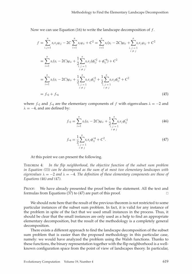
Now we can use Equation (16) to write the landscape decomposition of f .
f =n∑
i,j=1
sisjϕij − 2C
n∑i=1
siϕii + C2 =n∑
i=1
si(si − 2C)ϕii +n∑
i, j = 1i �= j
sisjϕij + C2
=n∑
i=1
si(si − 2C)ϕii + 12
n∑i, j = 1i �= j
sisj (φ-2ij + φ-4
ij ) + C2
=n∑
i=1
si(si − 2C)ϕii + 12
n∑i, j = 1i �= j
sisjφ-2ij + 1
2
n∑i, j = 1i �= j
sisjφ-4ij + C2
= f-2 + f-4 (45)
where f-2 and f-4 are the elementary components of f with eigenvalues λ = −2 andλ = −4, and are defined by:
f-2 =n∑
i=1
si(si − 2C)ϕii + 12
n∑i, j = 1i �= j
sisjφ-2ij (46)
f-4 = 12
n∑i, j = 1i �= j
sisjφ-4ij + C2. (47)
At this point we can present the following.
THEOREM 4: In the flip neighborhood, the objective function of the subset sum problemin Equation (15) can be decomposed as the sum of at most two elementary landscapes witheigenvalues λ = −2 and λ = −4. The definition of these elementary components are those ofEquations (46) and (47).
PROOF: We have already presented the proof before the statement. All the text andformulas from Equations (37) to (47) are part of this proof. �
We should note here that the result of the previous theorem is not restricted to someparticular instances of the subset sum problem. In fact, it is valid for any instance ofthe problem in spite of the fact that we used small instances in the process. Thus, itshould be clear that the small instances are only used as a help to find an appropriateelementary decomposition, but the result of the methodology is a completely generaldecomposition.
There exists a different approach to find the landscape decomposition of the subsetsum problem that is easier than the proposed methodology in this particular case,namely: we would have analyzed the problem using the Walsh functions. Thanks tothese functions, the binary representation together with the flip neighborhood is a well-known configuration space from the point of view of landscapes theory. In particular,
Evolutionary Computation Volume 19, Number 4 619

F. Chicano, L. D. Whitley, and E. Alba
it is known that any function with the form f (x) = ∏kj=1 xij can be decomposed in
at most k elementary landscapes, where all the ij holds 1 ≤ ij ≤ n (Rana et al., 1998).Furthermore, the eigenvalues of the elementary landscapes are −2p for 1 ≤ p ≤ k.Since the cost function of the subset sum problem is a quadratic polynomial of the xi
variables, it can be decomposed in at most two landscapes with eigenvalues −2 and−4. The elementary components of the cost function can be obtained by using someproperties of the Walsh functions. In the next section, we apply the methodology to amore complex example: the quadratic assignment problem (QAP).
4 A Complex Example: Quadratic Assignment Problem
The QAP is an NP-hard combinatorial optimization problem (Garey and Johnson, 1979).This problem class has a considerable importance since some other problems can be for-mulated as special cases of the QAP. One important example is the traveling salesmanproblem (TSP). The QAP is not an elementary landscape when the swap neighborhoodis considered (Angel and Zissimopoulos, 2000a). The solutions for this problem are per-mutations, and thus the usual neighborhood is the swap neighborhood. We also knowthat there exist orthogonal bases of eigenvectors for this configuration space (Stadler,2002). However, they are based on advanced concepts of group theory, so a specializedmathematical knowledge is required to deal with the Fourier expansion of QAP. Incontrast to this, the methodology presented here requires only basic concepts of linearalgebra. Part of the following derivation was previously outlined in a conference pa-per by Chicano et al. (2010); in the current paper, we show in detail the parts of thederivation omitted in the cited work.
4.1 QAP Formulation
Let P be a set of n facilities and L a set of n locations. For each pair of locations i and j , anarbitrary distance is specified rij and for each pair of facilities p and q, a flow is specifiedwpq . The QAP consists of assigning the facilities of P to the locations in L in such a waythat the total cost of the assignment is minimized. Each location can only contain onefacility and all the facilities must be assigned to a location. For each pair of facilities, thecost is computed as the product of the flow associated to the facilities and the distancebetween the locations in which the facilities are placed. The total cost is the sum of allthe costs associated to each pair of facilities. One solution to this problem is a bijectionbetween L and P , that is, x : L → P such that x is bijective. Without loss of generalitywe can just assume that P = L = {1, 2, . . . , n} and that each solution x is a permutationin Sn, the set permutations of {1, 2, . . . , n}. The cost function to be minimized can beformally defined as:
f (x) =n∑
i,j=1
rijwx(i)x(j ). (48)
The neighborhood N considered here is the swap or two-exchange neighborhood,in which two solutions are neighboring if one can be obtained from the other by a swap(exchange of two elements) in the permutation. Formally, y ∈ N (x) if and only if thereexist two different facilities i, j ∈ P such that y(i) = x(j ), y(j ) = x(i) and for all the otherfacilities k it holds y(k) = x(k).
620 Evolutionary Computation Volume 19, Number 4

Methodology to Find the Elementary Landscape Decomposition
4.2 Step 1: Rewrite the Objective Function
Let us start rewriting Equation (48). In the case of QAP, the information related to theparticular instance is included in the distance matrix (rij ) and the flow matrix (wpq).It is not difficult to see that Equation (48) can be written using the following linearcombination:
f (x) =n∑
i,j=1
n∑p,q=1
rijwpqδp
x(i)δq
x(j ) (49)
where we used the Kronecker delta. At this point we can go further and deal witha more general objective function. In Equation (49), the value of the product rijwpq
depends on i, j , p, and q in a particular way, but it is not the most general one. Usingmultilinear algebra concepts, the previous product is a four-rank tensor that has beencomputed as a tensor product of two two-rank tensors (matrices), which is a specialcase of a four-rank tensor. In the most general case, we can define a four-rank tensor toreplace the product. Let us call the new general four-rank tensor ψijpq and let us definethe parameterized basic function ϕ(i,j ),(p,q)(x) = δ
p
x(i)δq
x(j ). Then we can rewrite the fitnessfunction as:
f =n∑
i,j,p,q=1
ψijpqϕ(i,j ),(p,q) (50)
and we can focus our analysis on the family of basic functions ϕ(i,j ),(p,q). Now, theobjective function of the QAP is just a particular case of our new objective function f ,in which ψijpq = rijwpq .
Let us identify the equivalence classes in the set of the basic functions. If i �= j andp = q, then ϕ(i,j ),(p,q) = 0, and we can discard these functions. On the other hand, forall the pairs of functions ϕ(i,j ),(p,q) and ϕ(i ′,j ′),(p′,q ′) in which i �= j , p �= q, i ′ �= j ′, p′ �= q ′,we can find an automorphism π in the configuration graph G such that ϕ(i ′,j ′),(p′,q ′) =ϕ(i,j ),(p,q) ◦ π . In particular, if q �= p′, p �= q ′, j �= i ′, and i �= j ′, the automorphism π isdefined as:
π (x) = (i i ′) · (j j ′) · x · (p p′) · (q q ′) (51)
where we used the cycle representation of permutations, the terms with the parenthesesare swaps, and the dot operator represents the permutation composition. Then, all thefunctions ϕ(i,j ),(p,q) in which i �= j (and p �= q) are equivalent. We can focus our analysisjust on one of them, for example, ϕ(1,2),(1,2).
If i = j and p �= q we have ϕ(i,j ),(p,q) = 0 and, again, we can discard these functions.The functions ϕ(i,i),(p,p) are not equivalent to any function ϕ(i,j ),(p,q) in which i �= j ,since the number of solutions with ϕ = 1 is (n − 1)! in the first case and (n − 2)! in thesecond case. But are all the ϕ(i,i),(p,p) functions equivalent? The answer is yes, becauseϕ(i ′,i ′),(p′,p′) = ϕ(i,i),(p,p) ◦ π with the automorphism π (x) = (i i ′) · x · (p p′). Finally, we canfocus the next steps on the two basic functions ϕ(1,1),(1,1) and ϕ(1,2),(1,2). In order to simplifythe notation and when there is no ambiguity, we denote by ϕ1 the first function and byϕ2 the second function.
Evolutionary Computation Volume 19, Number 4 621

F. Chicano, L. D. Whitley, and E. Alba
Table 4: Elementary landscape decomposition of the basic functions ϕ1 and ϕ2 forn = 2, 3, 4, 5. We show the number of elementary components, the notation used forthem, and their eigenvalue.
Function n = 2 n = 3 n = 4 n = 5
ϕ1 φ−212 φ−3
13 φ−414 φ−5
15
ϕ2 φ−222 φ−3
23 , φ−623 φ−4
24 , φ−624 , φ−8
24 φ−525 , φ−8
25 , φ−1025
4.3 Step 2: Compute � and ϕ for Small Instances
In the QAP, an instance with n facilities has |X| = n! solutions. Thus, only a few smallinstances can be used in order to keep all the computations tractable. In particular,we use the values n = 2, 3, 4, 5. When n = 5, the Laplacian matrix is 120 × 120 and thecomputer algebra system requires some minutes to compute the eigensystem. We onlyshow here the Laplacians and the �ϕ vectors when n ≤ 3 for illustration purposes.
�2 =(−1 1
1 −1
)(52)
�3 =
⎛⎜⎜⎜⎜⎜⎜⎜⎜⎜⎜⎜⎜⎝
−3 1 1 1 0 0
1 −3 0 0 1 1
1 0 −3 0 1 1
1 0 0 −3 1 1
0 1 1 1 −3 0
0 1 1 1 0 −3
⎞⎟⎟⎟⎟⎟⎟⎟⎟⎟⎟⎟⎟⎠
(53)
�ϕ1 = �ϕ2 = (1, 0)T for n = 2 (54)
�ϕ1 = (1, 0, 0, 1, 0, 0)T �ϕ2 = (1, 0, 0, 0, 0, 0)T for n = 3. (55)
4.4 Step 3: Compute the Projections of ϕ in the Eigenspaces of �
Using a computer algebra system, we computed the projections of ϕ1 and ϕ2 into theeigenspaces of �. In Table 4 we show the eigenfunctions obtained for each basic functionϕi and each dimension n using the notation φλ
in, where λ is the eigenvalue.For illustration purposes we only show the projections of ϕ1 and ϕ2 for n ≤ 3.
φ-212 = φ-2
22 = 12
(1,−1)T ; φ-313 = 1
3(2,−1,−1, 2,−1,−1)T (56)
φ-323 = 1
3(2, 0, 0, 0,−1,−1)T ; φ-6
23 = 16
(1,−1,−1,−1, 1, 1)T . (57)
622 Evolutionary Computation Volume 19, Number 4
Methodology to Find the Elementary Landscape Decomposition
4.5 Step 4: Analyze the Projections and Propose Elementary Components
Once we know the elementary components of the basic functions for the small instances,we need to propose a general formula for the elementary components. First, we multiplythe φ functions by the smaller positive integer that makes integral all the componentsof the function. Then, we subtract the most common integer number in order to obtainthe greatest number of zeros in the function. This step is not necessary, but it is usefulfor finding a general rule for the φ functions. We must recall here that this step ofthe methodology requires, in principle, human intervention and for this reason it isappropriate to highlight noncommon values in the φ functions. This is what we didwith the previous operations.
With the help of Table 4 and the reduced graphs, we can establish a connectionbetween the elementary components in the different instances. For example, accordingto Table 4, the basic function ϕ1 is an elementary landscape for n ≤ 5 with eigenvalueλ = −n. We conjecture that this is also true for n ≥ 6. Regarding the second basic functionϕ2, we can conjecture that it is composed by at most three elementary landscapes forany problem size n. We observe in Table 4 that the cases n = 2 and n = 3 are special,since ϕ2 is elementary in the first case and the sum of two elementary components inthe second case. We will return later to these special cases.
If we analyze the eigenvalues of the elementary components, we observe that foreach problem instance the smallest one increases linearly with n. In particular, the linearrelationship is λ = −n. The same happens with the largest eigenvalue of each instancein which n ≥ 3, in this case the linear equation is λ = −2n. For n = 4 and n = 5, a thirdelementary component appears. Let us suppose that the eigenvalue of this elementarycomponent also increases linearly with n, then it should be λ = −2(n − 1). Now wemake the assumption that φ-2
22, φ-323, φ-4
24, and φ-525 are instances of a more general function
that is an elementary component for any size n of the problem. We further conjecturethat φ-6
23, φ-824, and φ-10
25 are instances of a different function that is also an elementarycomponent. Finally, we conjecture that φ-6
24 and φ-825 are instances of a third elementary
component. None of these assumptions need to be true (the truth of the assumptionswill be studied in the last step of the methodology), we are just proposing generalelementary components to be checked in the next step. Moreover, at this point of themethodology, there is no strong argument against the assumption that φ-3
23 and φ-624
are instances of the same elementary component. The check of the fifth step of themethodology will clarify this.
At this point, we conjecture that ϕ2 can be decomposed in at most three elementarylandscapes with eigenvalues −n, −2n, and −2(n − 1). Now we have to propose theexpressions for these elementary components in a general instance of size n. The reducedgraphs will be helpful for this task. For illustration purposes we show in Figure 7 thereduced graphs for φ-4
24 and φ-525. The interested reader can find the remaining reduced
graphs in Appendix A. We should find connections between the nodes of the reducedgraphs for the same elementary component in different instances. This we do in thefollowing.
Let us focus on the hypothetical elementary component with eigenvalue −n, de-noted as φ-n
2n . The reduced graphs of φ-424 and φ-5
25 are isomorphic and have five differentnodes. This means that the general elementary component most probably will takeat most five values. We can examine the solutions in each equivalence class of thegraphs in order to search for a connection between the nodes of the two graphs. Thenodes with labels −3 and −4 in the reduced graphs of φ-4
24 and φ-525, respectively, could
Evolutionary Computation Volume 19, Number 4 623
F. Chicano, L. D. Whitley, and E. Alba
Figure 7: Reduced graphs for φ-424 (left) and φ-5
25 (right).
Table 5: Equivalence classes of nodes labeled with −3 in the reduced graph of φ-424 and
with −4 in the reduced graph of φ-525.
Node −3 of φ-424 Node −4 of φ-5
25
[3,4,1,2] [3,5,4,2,1] [5,4,3,1,2] [3,4,1,2,5] [5,3,1,2,4] [3,4,2,5,1][3,4,2,1] [5,4,1,2,3] [5,3,2,4,1] [5,4,1,3,2] [5,4,2,1,3] [4,5,2,3,1][4,3,1,2] [5,3,4,1,2] [3,4,1,5,2] [5,3,2,1,4] [4,3,5,1,2] [3,5,4,1,2][4,3,2,1] [4,5,1,3,2] [3,5,1,2,4] [4,3,2,5,1] [4,5,3,2,1] [3,4,5,1,2]
[4,3,1,5,2] [3,5,1,4,2] [5,4,2,3,1] [5,4,3,2,1] [3,4,2,1,5][3,5,2,4,1] [4,3,2,1,5] [4,5,2,1,3] [5,3,1,4,2] [4,3,1,2,5][3,5,2,1,4] [5,3,4,2,1] [4,5,3,1,2] [3,4,5,2,1] [4,3,5,2,1][4,5,1,2,3]
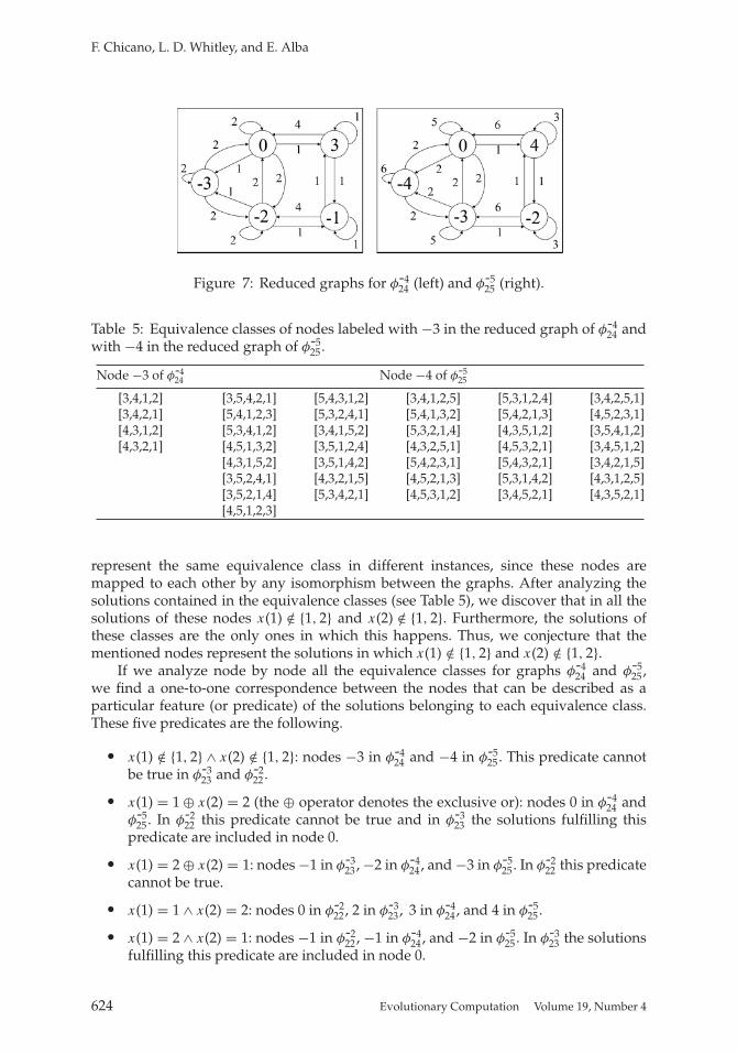
represent the same equivalence class in different instances, since these nodes aremapped to each other by any isomorphism between the graphs. After analyzing thesolutions contained in the equivalence classes (see Table 5), we discover that in all thesolutions of these nodes x(1) /∈ {1, 2} and x(2) /∈ {1, 2}. Furthermore, the solutions ofthese classes are the only ones in which this happens. Thus, we conjecture that thementioned nodes represent the solutions in which x(1) /∈ {1, 2} and x(2) /∈ {1, 2}.
If we analyze node by node all the equivalence classes for graphs φ-424 and φ-5
25,we find a one-to-one correspondence between the nodes that can be described as aparticular feature (or predicate) of the solutions belonging to each equivalence class.These five predicates are the following.
• x(1) /∈ {1, 2} ∧ x(2) /∈ {1, 2}: nodes −3 in φ-424 and −4 in φ-5
25. This predicate cannotbe true in φ-3
23 and φ-222.
• x(1) = 1 ⊕ x(2) = 2 (the ⊕ operator denotes the exclusive or): nodes 0 in φ-424 and
φ-525. In φ-2
22 this predicate cannot be true and in φ-323 the solutions fulfilling this
predicate are included in node 0.
• x(1) = 2 ⊕ x(2) = 1: nodes −1 in φ-323, −2 in φ-4
24, and −3 in φ-525. In φ-2
22 this predicatecannot be true.
• x(1) = 1 ∧ x(2) = 2: nodes 0 in φ-222, 2 in φ-3
23, 3 in φ-424, and 4 in φ-5
25.
• x(1) = 2 ∧ x(2) = 1: nodes −1 in φ-222, −1 in φ-4
24, and −2 in φ-525. In φ-3
23 the solutionsfulfilling this predicate are included in node 0.
624 Evolutionary Computation Volume 19, Number 4

Methodology to Find the Elementary Landscape Decomposition
In the previous classification we observe that the labels of the nodes in each equiv-alence class change in a linear way with respect to n. The only exception is that of φ-2
22.Then, we take into account this fact to propose a general expression for φ-n
2n when n ≥ 3.The proposal is the following:
φ-n2n =
⎧⎪⎪⎪⎪⎪⎪⎪⎪⎨⎪⎪⎪⎪⎪⎪⎪⎪⎩
n − 1 if x(i) = p ∧ x(j ) = q
3 − n if x(i) = q ∧ x(j ) = p
0 if x(i) = p ⊕ x(j ) = q
2 − n if x(i) = q ⊕ x(j ) = p
1 − n if x(i) /∈ {p, q} ∧ x(j ) /∈ {p, q}
(58)
where we now again use i �= j instead of 1 and 2, and we also again introduce the p �= q.Equation (58) is a hypothetical elementary component of the basic function ϕ(i,j ),(p,q)where i �= j and p �= q. We previously saw that φ-2
22 = φ-212 are elementary landscapes.
Thus, we can treat n = 2 as a special case in which the QAP is an elementary landscapedue to the elementariness of φ-2
12 and φ-222.
Let us now focus on the hypothetical elementary component with eigenvalue −2n,denoted with φ-2n
2n . The reduced graphs of φ-824 and φ-10
25 (shown in Appendix A) are iso-morphic and have five different nodes. Furthermore, they are isomorphic with φ-4
24 andφ-5
25. After examining the solutions in each node, we find that the equivalence classes arethe same as in the previous function φ-n
2n . We also observe that there is a linear relationshipbetween the values of the nodes and n. An analysis of the equivalence classes similar tothe one used for the φ-n
2n functions suggests the following proposal for φ-2n2n when n ≥ 3:
φ-2n2n =
⎧⎪⎪⎪⎪⎪⎪⎪⎪⎨⎪⎪⎪⎪⎪⎪⎪⎪⎩
n − 1 if x(i) = p ∧ x(j ) = q
3 − n if x(i) = q ∧ x(j ) = p
0 if x(i) = p ⊕ x(j ) = q
2 if x(i) = q ⊕ x(j ) = p
1 if x(i) /∈ {p, q} ∧ x(j ) /∈ {p, q}
. (59)
The previous proposal explains why the hypothetical elementary component φ-2n2n
is not present in ϕ2 when n = 2. The reason is that the three last branches of the functiondefinition cannot be true if n = 2 and for the two first branches the value of φ-4
22 is 1, sothe function is a constant function (elementary component with λ = 0), and its effect isa change in the average value of ϕ2.
Finally, let us focus on the hypothetical elementary component with eigenvalue−2(n − 1), denoted as φ
-2(n-1)2n . In this case, the reduced graphs of φ-6
24 and φ-825 are not
isomorphic. However, after examining the solutions in each node and analyzing the
Evolutionary Computation Volume 19, Number 4 625

F. Chicano, L. D. Whitley, and E. Alba
equivalence classes we find the following proposal for φ-2(n-1)2n when n ≥ 4:
φ-2(n-1)2n =
⎧⎪⎪⎪⎪⎪⎪⎪⎪⎨⎪⎪⎪⎪⎪⎪⎪⎪⎩
n − 3 if x(i) = p ∧ x(j ) = q
n − 3 if x(i) = q ∧ x(j ) = p
0 if x(i) = p ⊕ x(j ) = q
0 if x(i) = q ⊕ x(j ) = p
1 if x(i) /∈ {p, q} ∧ x(j ) /∈ {p, q}
(60)
where we used the same branching scheme of Equations (58) and (59) for clarity.The previous proposal explains why the hypothetical elementary component φ
-2(n-1)2n
is not present in ϕ2 when n = 2, 3. If n = 2 the three last branches of the functiondefinition cannot be true and for the two first branches the value is –1, so the functionis a constant function. If n = 3, the last branch cannot be true, and the remainingbranches take value 0, so the function is again a constant function.
At this point we have a proposal for the elementary components of all the basicfunctions ϕ(i,j ),(p,q). Now, in the next step we have to check that the proposed elementarycomponents are really elementary components and we need to compute the value of theweights that these elementary components have in the sum to give the basic functions.
4.6 Step 5: Check the Landscape Decomposition in the General Case
In this step, we check the decomposition deduced in the previous step. First, let us focuson the basic functions ϕ(i,i),(p,p). In the previous step, we conjectured that these basicfunctions are elementary with eigenvalue λ = −n. Let us study whether this is true withthe help of the characterization of elementary landscapes given by Proposition 2.
In the following, for the sake of clarity we will remove all the parameters from thename of the function when there is no confusion. The function ϕ is elementary if andonly if there exist two constants a and b such that the following expression holds for allthe solutions:
avg{ϕ(y)}y∈N(x)
= aϕ(x) + b.
In order to reduce the expressions, we multiply the previous expression by the size ofthe neighborhood, which is d = n(n−1)
2 . We then obtain:
∑y∈N(x)
ϕ(y) = cϕ(x) + e (61)
where c = ad and e = bd. Next, we compute the exact expression of∑
y∈N(x) ϕ(y) for thetwo different values that ϕ can take:
• Case ϕ(x) = 1 (in this case x(i) = p). From the neighboring solutions, there aren − 1 with ϕ(y) = 0 and the remaining neighbors have a value ϕ(y) = 1. Then wecan write: ∑
y∈N(x)
ϕ(y) = (d − n + 1).
626 Evolutionary Computation Volume 19, Number 4

Methodology to Find the Elementary Landscape Decomposition
• Case ϕ(x) = 0 (in this case x(i) �= p). From the neighboring solutions there is onlyone with ϕ(y) = 1. The remaining neighbors have a value ϕ(y) = 0. Then we canwrite: ∑
y∈N(x)
ϕ(y) = 1.
Now we use Equation (61) to obtain the following linear equation system:
(1 1
0 1
) (c
e
)=
(d − n + 1
1
).
The solution of the previous system is c = d − n and e = 1; so we have a = 1 − n/d
and b = 1/d. We conclude that ϕ(i,i),(p,p) is an elementary landscape with λ = −n.Now, let us focus on the landscape decomposition of ϕ(i,j ),(p,q) for i �= j and p �= q.
Our conjecture in this case is that this function is a weighted sum of the three hypo-thetical elementary components defined in Equations (58), (59), and (60). We first haveto prove that the hypothetical elementary components are really elementary compo-nents in the general case. We will exploit the similar structure of the three functions toprove their elementariness at the same time. With this aim, let us define the followingparameterized function:
φα,β,γ,ε,ζ
(i,j ),(p,q)(x) =
⎧⎪⎪⎪⎪⎪⎪⎪⎪⎨⎪⎪⎪⎪⎪⎪⎪⎪⎩
α if x(i) = p ∧ x(j ) = q
β if x(i) = q ∧ x(j ) = p
γ if x(i) = p ⊕ x(j ) = q
ε if x(i) = q ⊕ x(j ) = p
ζ if x(i) /∈ {p, q} ∧ x(j ) /∈ {p, q}
(62)
where 1 ≤ i, j, p, q ≤ n are integer values with i �= j and p �= q and α, β, γ, ε, ζ ∈ R. InFigure 8 we show the reduced graph of this parameterized function. Again, using theconcept of equivalence of solutions, we can prove that the graph in this figure is thereduced graph for φ
α,β,γ,ε,ζ
(i,j ),(p,q). For example, in node α the solutions satisfy the conditionx(i) = p ∧ x(j ) = q. Such solutions have exactly one neighbor in node β (obtained byswapping positions i and j ), 2(n − 2) solutions in node γ (swapping either i or j
with a third position k), and the remaining solutions in α (when positions i and j
are unaffected). This analysis can be extended to the remaining nodes and we finallyconclude that it is a reduced graph.
We should note, however, that depending on the values of the parameters α, β, γ ,ε, and ζ it would be possible to collapse some nodes in the graph. For example, if α = β
and γ = ε, we would collapse the corresponding nodes obtaining a three-node reducedgraph. Thus, the graph of Figure 8 is not always the reduced graph. Fortunately, thisis not important, because we do not need the reduced graph for the proof, but a graphsmall enough having different equivalence classes in different nodes. It does not matterif one equivalence class is scattered in different nodes.
Again, for the sake of clarity we will remove all the parameters from the name ofthe function when there is no confusion. The function φ is elementary if and only if
Evolutionary Computation Volume 19, Number 4 627

F. Chicano, L. D. Whitley, and E. Alba
Figure 8: Reduced graph for φα,β,γ,ε,ζ
(i,j ),(p,q).
there exist two constants a and b such that the following expression holds for all thesolutions:
avg{φ(y)}y∈N(x)
= aφ(x) + b.
In order to reduce the expressions we multiply the previous expression by the size ofthe neighborhood, which is d = n(n−1)
2 . We then obtain:
∑y∈N(x)
φ(y) = cφ(x) + e (63)
where c = ad and e = bd.Next, we compute the exact expression of
∑y∈N(x) φ(y) for the five different values
that φ can take:
• Case φ(x) = α. In this case x(i) = p and x(j ) = q. From the neighboring solutionsthere is one with φ(y) = β and 2(n − 2) solutions with φ(y) = γ . The remainingneighbors have a value φ(y) = α. Then we can write:
∑y∈N(x)
φ(y) = β + 2(n − 2)γ + (d − 2n + 3)α.
• Case φ(x) = β. In this case x(i) = q and x(j ) = p. From the neighboring solutionsthere is one with φ(y) = α and 2(n − 2) solutions with φ(y) = ε. The remainingneighbors have a value φ(y) = β. Then we can write:
∑y∈N(x)
φ(y) = α + 2(n − 2)ε + (d − 2n + 3)β.
• Case φ(x) = γ . In this case x(i) = p or x(j ) = q, but not both. From the neighboringsolutions there is one with φ(y) = α, two neighbors with φ(y) = ε, and n − 3
628 Evolutionary Computation Volume 19, Number 4

Methodology to Find the Elementary Landscape Decomposition
neighbors with φ(y) = ζ . The remaining neighbors have a value φ(y) = γ . Thenwe can write:
∑y∈N(x)
φ(y) = α + 2ε + (n − 3)ζ + (d − n)γ.
• Case φ(x) = ε. In this case, x(i) = q or x(j ) = p, but not both. From the neighboringsolutions there is one with φ(y) = β, two neighbors with φ(y) = γ , and n − 3neighbors with φ(y) = ζ . The remaining neighbors have a value φ(y) = ε. Thenwe can write:
∑y∈N(x)
φ(y) = β + 2γ + (n − 3)ζ + (d − n)ε.
• Case φ(x) = ζ . In this case, x(i) /∈ {p, q} and x(j ) /∈ {p, q}. From the neighboringsolutions there are two with φ(y) = γ and two neighbors with φ(y) = ε. Theremaining neighbors have a value φ(y) = ζ . Then we can write:∑
y∈N(x)
φ(y) = 2γ + 2ε + (d − 4)ζ.
We use Equation (63) to obtain the following system of linear equations.
⎛⎜⎜⎜⎜⎜⎜⎜⎜⎝
α 1
β 1
γ 1
ε 1
ζ 1
⎞⎟⎟⎟⎟⎟⎟⎟⎟⎠
(c
e
)=
⎛⎜⎜⎜⎜⎜⎜⎜⎜⎝
β + 2(n − 2)γ + (d − 2n + 3)α
α + 2(n − 2)ε + (d − 2n + 3)β
α + 2ε + (n − 3)ζ + (d − n)γ
β + 2γ + (n − 3)ζ + (d − n)ε
2γ + 2ε + (d − 4)ζ
⎞⎟⎟⎟⎟⎟⎟⎟⎟⎠
.
The previous system has five equations and two variables, c and e, so it could beunsolvable. However, the system can be solved for some value combinations of α, β, γ ,ε, ζ . In particular, the system can be solved for the value combinations we are interestedin, that is:
1. α = n − 1, β = 3 − n, γ = 0, ε = 2 − n, ζ = 1 − n (function φ-n2n)
2. α = n − 1, β = 3 − n, γ = 0, ε = 2, ζ = 1 (function φ-2n2n )
3. α = n − 3, β = n − 3, γ = 0, ε = 0, ζ = 1 (function φ-2(n-1)2n )
This does not mean that these are the only combinations of parameter values forwhich the system can be solved. They are just three combinations of special interest forthe goal of this section. It should be noted here that the linear system does not dependon the values of i, j , p, and q. Thus, the solutions to the system are also independent ofthe values of the mentioned parameters.
Let us study the values of a, b, c, and e for the first parameter combination, thatis, α = n − 1, β = 3 − n, γ = 0, ε = 2 − n, and ζ = 1 − n. The solution of the linear
Evolutionary Computation Volume 19, Number 4 629
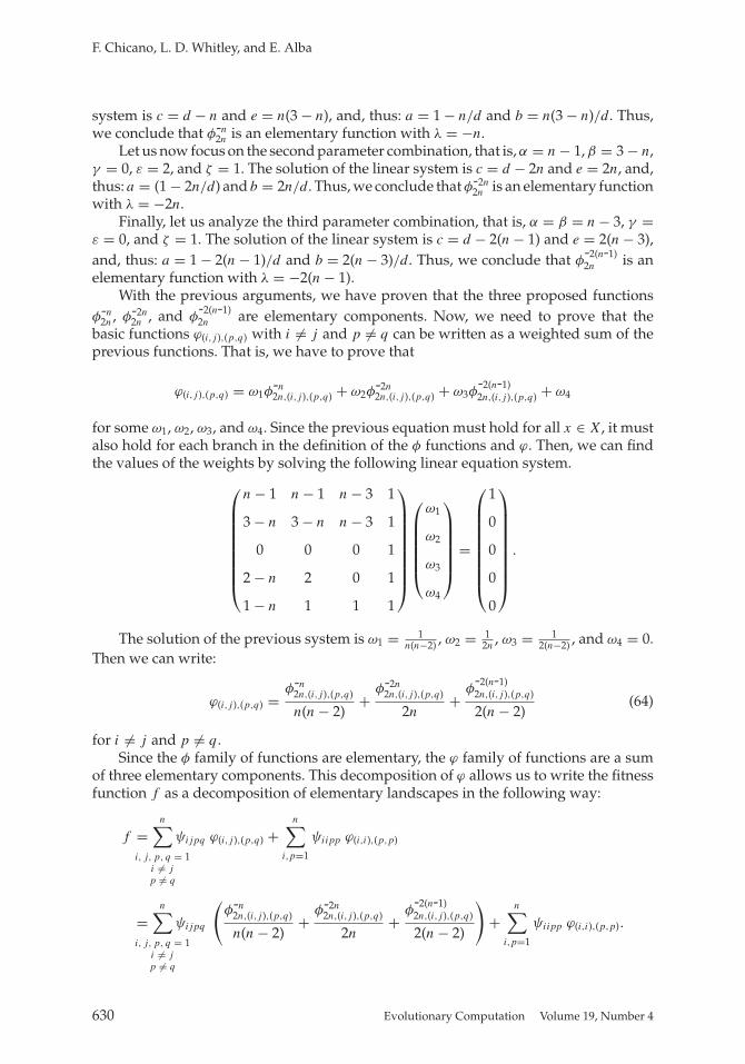
F. Chicano, L. D. Whitley, and E. Alba
system is c = d − n and e = n(3 − n), and, thus: a = 1 − n/d and b = n(3 − n)/d. Thus,we conclude that φ-n
2n is an elementary function with λ = −n.Let us now focus on the second parameter combination, that is, α = n − 1, β = 3 − n,
γ = 0, ε = 2, and ζ = 1. The solution of the linear system is c = d − 2n and e = 2n, and,thus: a = (1 − 2n/d) and b = 2n/d. Thus, we conclude that φ-2n
2n is an elementary functionwith λ = −2n.
Finally, let us analyze the third parameter combination, that is, α = β = n − 3, γ =ε = 0, and ζ = 1. The solution of the linear system is c = d − 2(n − 1) and e = 2(n − 3),and, thus: a = 1 − 2(n − 1)/d and b = 2(n − 3)/d. Thus, we conclude that φ
-2(n-1)2n is an
elementary function with λ = −2(n − 1).With the previous arguments, we have proven that the three proposed functions
φ-n2n , φ-2n
2n , and φ-2(n-1)2n are elementary components. Now, we need to prove that the
basic functions ϕ(i,j ),(p,q) with i �= j and p �= q can be written as a weighted sum of theprevious functions. That is, we have to prove that
ϕ(i,j ),(p,q) = ω1φ-n2n,(i,j ),(p,q) + ω2φ
-2n2n,(i,j ),(p,q) + ω3φ
-2(n-1)2n,(i,j ),(p,q) + ω4
for some ω1, ω2, ω3, and ω4. Since the previous equation must hold for all x ∈ X, it mustalso hold for each branch in the definition of the φ functions and ϕ. Then, we can findthe values of the weights by solving the following linear equation system.⎛
⎜⎜⎜⎜⎜⎜⎜⎜⎝
n − 1 n − 1 n − 3 1
3 − n 3 − n n − 3 1
0 0 0 1
2 − n 2 0 1
1 − n 1 1 1
⎞⎟⎟⎟⎟⎟⎟⎟⎟⎠
⎛⎜⎜⎜⎜⎜⎝
ω1
ω2
ω3
ω4
⎞⎟⎟⎟⎟⎟⎠ =
⎛⎜⎜⎜⎜⎜⎜⎜⎜⎝
1
0
0
0
0
⎞⎟⎟⎟⎟⎟⎟⎟⎟⎠
.
The solution of the previous system is ω1 = 1n(n−2) , ω2 = 1
2n, ω3 = 1
2(n−2) , and ω4 = 0.Then we can write:
ϕ(i,j ),(p,q) =φ-n
2n,(i,j ),(p,q)
n(n − 2)+
φ-2n2n,(i,j ),(p,q)
2n+
φ-2(n-1)2n,(i,j ),(p,q)
2(n − 2)(64)
for i �= j and p �= q.Since the φ family of functions are elementary, the ϕ family of functions are a sum
of three elementary components. This decomposition of ϕ allows us to write the fitnessfunction f as a decomposition of elementary landscapes in the following way:
f =n∑
i, j, p, q = 1i �= j
p �= q
ψijpq ϕ(i,j ),(p,q) +n∑
i,p=1
ψiipp ϕ(i,i),(p,p)
=n∑
i, j, p, q = 1i �= j
p �= q
ψijpq
(φ-n
2n,(i,j ),(p,q)
n(n − 2)+
φ-2n2n,(i,j ),(p,q)
2n+
φ-2(n-1)2n,(i,j ),(p,q)
2(n − 2)
)+
n∑i,p=1
ψiipp ϕ(i,i),(p,p).
630 Evolutionary Computation Volume 19, Number 4
Methodology to Find the Elementary Landscape Decomposition
The elementary components of f are:
f-n = 1n(n − 2)
n∑i, j, p, q = 1
i �= j
p �= q
ψijpq φ-n2n,(i,j ),(p,q) +
n∑i,p=1
ψiipp ϕ(i,i),(p,p) (65)
f-2n = 12n
n∑i, j, p, q = 1
i �= j
p �= q
ψijpq φ-2n2n,(i,j ),(p,q) (66)
f-2(n-1) = 12(n − 2)
n∑i, j, p, q = 1
i �= j
p �= q
ψijpq φ-2(n-1)2n,(i,j ),(p,q) (67)
where the functions f-n, f-2n, and f-2(n-1) are elementary with eigenvalues λ1 = −n,λ2 = −2n, and λ3 = −2(n − 1), respectively, because they are a linear combination ofelementary functions. Thus, f can be written in a compact form as:
f = f−n + f-2n + f-2(n-1). (68)
Equations (65) to (67) are valid if n ≥ 3. If n = 2, there are only two solutions inthe search space and the objective function is elementary with eigenvalue λ = −2 sinceit can be written as a linear combination of ϕ(i,i),(p,p) functions. At this point we canpresent the following.
THEOREM 5: In the swap neighborhood the objective function of the QAP in Equation (48) canbe decomposed as the sum of at most three elementary landscapes with eigenvalues λ1 = −n,λ2 = −2n, and λ3 = −2(n − 1). The definition of these elementary components are those ofEquations (65), (66), and (67).
PROOF: Again we have presented the proof before the statement. The content of thefifth step of the methodology is the proof. �
As stated in the previous theorem, the number of elementary components of QAPcannot be larger than three, but it could be lower. For example, we have observedduring the application of the methodology that if n = 2 the QAP is elementary and ifn = 3 there are at most two elementary components with different eigenvalues. It isalso possible that for some particular instances the number of elementary landscapescould be reduced. For example, the symmetric TSP is a particular subclass of the QAPthat is elementary, the antisymmetric TSP is elementary, and the general asymmetricTSP is the sum of at most two elementary landscapes (Barnes et al., 2002; Stadler,1996).
Evolutionary Computation Volume 19, Number 4 631
F. Chicano, L. D. Whitley, and E. Alba
In Appendix B we show the application of the elementary landscape decompo-sition of the QAP to compute the autocorrelation function of some instances of theQAPLIB (Burkard et al., 1997). We observe that using the elementary landscape decom-position, the autocorrelation values can be computed much faster than using experi-mental statistical methods.
5 Limitations of the Methodology
The methodology presented in this paper is very useful, but it also has limitations.First, it works under the assumption that the number of elementary components of anyinstance of the problem is bounded by a small constant. This happens in many com-binatorial optimization problems, like the subset sum problem, the TSP, or the QAP.But there also exist some problems in which this assumption is not true, like the max-imum satisfiability problem (MAX-SAT) or the NK landscapes. An analysis based onFourier expansions reveals that the maximum number of elementary components inMAX-SAT is the maximum number of literals appearing in any clause, and the maxi-mum number of elementary components in the NK landscapes is K + 1 (Sutton et al.,2009). Thus, the maximum number of elementary components in any of these prob-lems depends on the particular instance being solved. If our methodology is appliedto these problems, the variable number of elementary components could go unnoticed.At the moment we have no rule to guess how many elementary components a functionhas and we cannot predict from a problem definition whether it can be easily decom-posed using the methodology proposed or not. Finding such rules is a line of futurework.
Second, the methodology requires human intervention to propose the elementarycomponents, so it depends on the human skills to identify the equivalence classesbetween the different reduced graphs of different instances. However, as far as weknow no methodology exists for decomposing a combinatorial optimization probleminto elementary components that can obviate human intervention. Thus, this limitationis not particular to our methodology but general. A fully automated approach wouldbe preferable, but it would also require complete information of the problem andits representation. Our methodology, however, is based on limited knowledge of theproblem: Only a few instances of the problem are analyzed and no information ofthe internal structure of the solutions is used in the systematic steps. We think thatthis second limitation could be alleviated by using heuristic algorithms to automatethe proposal of general elementary components. It is our experience that most of theelementary components are clear after observing the elementary components of thebasic functions for small instances. We could program this experience in the form ofheuristic algorithms that could suggest to a researcher the general components of alandscape.
Finally, the success of the methodology depends to a large extent on the growth ofthe search space with the problem size. The methodology requires explicitly dealingwith some particular instances of the problem. Only the smallest ones can be usedbecause the size of the search space increases exponentially with the parameters of theinstances. This is a consequence of the explicit representation of the basic functions and,specially, the Laplacian matrix. The computation of the eigensystem of the Laplacianrequires a computational effort that increases with the Laplacian size. We think that onesolution to this problem could be the symbolic manipulation of the Laplacian and thebasic functions.
632 Evolutionary Computation Volume 19, Number 4

Methodology to Find the Elementary Landscape Decomposition
6 Conclusion and Future Work
In this paper we have made three contributions. First, we have presented new theo-retical results on landscapes theory that generalize our understanding of elementarylandscapes and their properties. Second, we have developed a methodology basedon linear algebra that can potentially be used to find a decomposition of a functioninto a linear combination of elementary components. This decomposition has practicaland theoretical applications. In practice, the decomposition allows one to compute theaverage value of the objective function in the neighborhood of any solution withoutevaluating all the solutions in the neighborhood. In theory, the decomposition opens thedoor to the exact computation of the autocorrelation functions and the autocorrelationlength in polynomial time. Finally, we have used the methodology to prove that thesubset sum problem is a superposition of two elementary landscapes, and the QAP is asuperposition of three elementary landscapes.
As future work we distinguish three different lines of research based on the method-ology proposed in this paper. First, we plan to apply the methodology to a large numberof combinatorial optimization problems for which the elementary landscape decompo-sition is not known. This decomposition is valuable itself, since it allows one to computethe autocorrelation coefficient for any instance of the problems and could be the basisfor new theoretical studies or new operators for evolutionary algorithms. Second, thetopic on how the elementary components of a problem can be used to improve thealgorithmic performance is an issue that deserves additional research. Third, it is pos-sible to automate most of the operations of the proposed methodology using specificsoftware tools and computer algebra systems. Moreover, we could group together allthese operations and develop a single software tool to support the elementary land-scape decomposition of a general landscape. Using this tool the researcher could focuson the main creative parts of the methodology: rewriting the objective function andproposing elementary components. We plan to develop such a tool.
Acknowledgments
We are grateful for the constructive comments from the anonymous reviewers of thispaper. This work has been partially funded by the Spanish Ministry of Science andInnovation and FEDER under contract TIN2008-06491-C04-01 (the M∗ project). It hasalso been partially funded by the Andalusian government under contract P07-TIC-03044 (DIRICOM project) and by the Air Force Office of Scientific Research, Air ForceMateriel Command, USAF, under grant number FA9550-08-1-0422. The U.S. govern-ment is authorized to reproduce and distribute reprints for governmental purposesnotwithstanding any copyright notation thereon.
References
Angel, E., and Zissimopoulos, V. (2000a). On the classification of NP-complete problems in termsof their correlation coefficient. Discrete Applied Mathematics, 99:261–277.
Angel, E., and Zissimopoulos, V. (2000b). On the landscape ruggedness of the quadratic assign-ment problem. Theoretical Computer Sciences, 263:159–172.
Barnes, J., Dokov, S., Acevedo, R., and Solomon, A. (2002). A note on distance matrices yieldingelementary landscapes for the TSP. Journal of Mathematical Chemistry, 31(2):233–235.
Evolutionary Computation Volume 19, Number 4 633
F. Chicano, L. D. Whitley, and E. Alba
Biyikoglu, T., Leyold, J., and Stadler, P. F. (2007). Laplacian eigenvectors of graphs. Lecture Notes inMathematics. Berlin: Springer-Verlag.
Burkard, R., Karisch, S., and Rendl, F. (1997). QAPLIB—A quadratic assignment problem library.Journal of Global Optimization, 10:391–403.
Chicano, F., Luque, G., and Alba, E. (2010). Elementary landscape decomposition of the quadraticassignment problem. In Proceedings of GECCO, pp. 1425–1432.
Codenotti, B., and Margara, L. (1992). Local properties of some NP-complete problems. TechnicalReport TR 92-021, International Computer Science Institute, Berkeley, CA.
Garcıa-Pelayo, R., and Stadler, P. (1997). Correlation length, isotropy and meta-stable states.Physica D: Nonlinear Phenomena, 107(2–4):240–254.
Garey, M. R., and Johnson, D. S. (1979). Computers and intractability: A guide to the theory ofNP-completeness. New York: W.H. Freeman.
Lu, G., Bahsoon, R., and Yao, X. (2010). Applying elementary landscape analysis to search-based software engineering. In Proceedings of the 2nd International Symposium on Search BasedSoftware Engineering, pp. 3–8.
Rana, S., Heckendorn, R. B., and Whitley, D. (1998). A tractable walsh analysis of SAT and itsimplications for genetic algorithms. In Proceedings of AAAI, pp. 392–397.
Reidys, C. M., and Stadler, P. F. (2002). Combinatorial landscapes. SIAM Review, 44(1):3–54.
Stadler, P. F. (1995). Toward a theory of landscapes. In R. Lopez-Pena, R. Capovilla, R. Garcıa-Pelayo, H. Waelbroeck, and F. Zertruche (Eds.), Complex systems and binary networks (pp.77–163). Berlin: Springer-Verlag.
Stadler, P. F. (1996). Landscapes and their correlation functions. Journal of Mathematical Chemistry,20:1–45.
Stadler, P. F. (2002). Fitness landscapes. In M. Lassig and A. Valleriani (Eds.), Biological evolutionand statistical physics (pp. 183–204). Berlin: Springer.
Sutton, A. M., Howe, A. E., and Whitley, L. D. (2010). Directed plateau search for MAX-k-SAT.Paper presented at The 3rd Annual Symposium on Combinational Search, SoCS.
Sutton, A. M., Whitley, L. D., and Howe, A. E. (2009). A polynomial time computation of theexact correlation structure of k-satisfiability landscapes. In Proceedings of GECCO, pp. 365–372.
Weinberger, E. (1990). Correlated and uncorrelated fitness landscapes and how to tell the differ-ence. Biological Cybernetics, 63(5):325–336.
Whitley, D., Sutton, A. M., and Howe, A. E. (2008). Understanding elementary landscapes. InProceedings of GECCO, pp. 585–592.
Whitley, L. D., and Sutton, A. M. (2009). Partial neighborhoods of elementary landscapes. InProceedings of GECCO, pp. 381–388.
Appendix A Reduced Graphs for Small Instances of QAP
In Figures 9 to 12 we show all the reduced graphs for the projections of ϕ1 and ϕ2 and2 ≤ n ≤ 5.
634 Evolutionary Computation Volume 19, Number 4

Methodology to Find the Elementary Landscape Decomposition
Figure 9: Reduced graphs for the projections of ϕ1 and ϕ2 when n = 2: φ-212 = φ-2
22.
Figure 10: Reduced graphs for the projections of ϕ1 and ϕ2 when n = 3: φ-313 (left),
φ-323 (center), and φ-6
23 (right).
Figure 11: Reduced graphs for the projections of ϕ1 and ϕ2 when n = 4: φ-414 (top left),
φ-424 (top right), φ-6
24 (bottom left), and φ-824 (bottom right).
Evolutionary Computation Volume 19, Number 4 635

F. Chicano, L. D. Whitley, and E. Alba
Figure 12: Reduced graphs for the projections of ϕ1 and ϕ2 when n = 5: φ-515 (top left),
φ-525 (top right), φ-8
25 (bottom left), and φ-1025 (bottom right).
Appendix B Autocorrelation of QAP
Let us consider an infinite random walk {x0, x1, . . .} on the solution space such that xi+1 ∈N (xi). The random walk autocorrelation function r : N → R is defined as (Weinberger, 1990):
r(s) = avg{f (xt )f (xt+s)}x0,t− avg{f (xt )}2
x0,t
avg{f (xt )2}x0,t
− avg{f (xt )}2x0,t
(69)
where the subindices x0 and t indicate that the averages are computed over all thestarting solutions x0 ∈ X and along the complete random walk.
The autocorrelation function r(s) can be computed from the actual problem data(instance) using the following expression (Chicano et al., 2010):
r(s) = W-n
(1 − 2
n − 1
)s
+ W-2n
(1 − 4
n − 1
)s
+ W-2(n-1)
(1 − 4
n
)s
(70)
where the coefficients Wλ, called spectral amplitudes, are defined after the elementarycomponents and f as
Wλ = f 2λ − fλ
2
f 2 − f2 . (71)
636 Evolutionary Computation Volume 19, Number 4
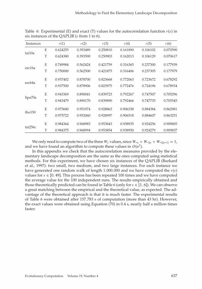
Methodology to Find the Elementary Landscape Decomposition
Table 6: Experimental (E) and exact (T) values for the autocorrelation function r(s) insix instances of the QAPLIB (s from 1 to 6).
Instances r(1) r(2) r(3) r(4) r(5) r(6)
E 0.624255 0.393489 0.250810 0.161890 0.106102 0.070590tai10a
T 0.624380 0.393590 0.250903 0.162013 0.106129 0.070617
E 0.749984 0.562424 0.421759 0.316365 0.237300 0.177939esc16a
T 0.750000 0.562500 0.421875 0.316406 0.237305 0.177979
E 0.937402 0.878700 0.823668 0.772063 0.723672 0.678292esc64a
T 0.937500 0.878906 0.823975 0.772476 0.724196 0.678934
E 0.943369 0.890041 0.839723 0.792267 0.747507 0.705296lipa70a
T 0.943479 0.890170 0.839890 0.792466 0.747735 0.705545
E 0.975680 0.951974 0.928863 0.906338 0.884384 0.862981tho150
T 0.975722 0.952060 0.928997 0.906518 0.884607 0.863251
E 0.984364 0.968983 0.953843 0.938935 0.924256 0.909805tai256c
T 0.984375 0.968994 0.953854 0.938950 0.924279 0.909837
We only need to compute two of the three Wλ values, since W-n + W-2n + W-2(n-1) = 1,and we have found an algorithm to compute these values in O(n2).
In this appendix we check that the autocorrelation measures provided by the ele-mentary landscape decomposition are the same as the ones computed using statisticalmethods. For this experiment, we have chosen six instances of the QAPLIB (Burkardet al., 1997): two small, two medium, and two large instances. For each instance wehave generated one random walk of length 1,000,000 and we have computed the r(s)values for s ∈ [0, 49]. This process has been repeated 100 times and we have computedthe average value for the 100 independent runs. The results empirically obtained andthose theoretically predicted can be found in Table 6 (only for s ∈ [1, 6]). We can observea great matching between the empirical and the theoretical value, as expected. The ad-vantage of the theoretical approach is that it is much faster. The experimental resultsof Table 6 were obtained after 157,783 s of computation (more than 43 hr). However,the exact values were obtained using Equation (70) in 0.4 s, nearly half a million timesfaster.
Evolutionary Computation Volume 19, Number 4 637