A Matter of Disorder: Monte Carlo Simulations of Phase ...

A Matter of Disorder: Monte CarloSimulations of Phase Transitions in Strongly

Disordered Systems

Marios Nikolaou

Doctoral ThesisKTH School of Engineering Sciences

Stockholm, Sweden 2007

TRITA-FYS 2007:19ISSN 0280-316XISRN KTH/FYS/--07:19--SEISBN 978-91-7178-600-5

KTH School of Engineering SciencesAlbaNova UniversitetscentrumSE-106 91 StockholmSweden

Akademisk avhandling som med tillstånd av Kungl Tekniska högskolan framlägges tilloffentlig granskning för avläggande av teknologie doktorsexamen i teoretisk fysik freda-gen den 30 mars 2007 klockan 10.15 i The Svedbergsalen, AlbaNova Universitetscent-rum, Kungl Tekniska högskolan, Roslagstullsbacken 21, Stockholm.

© Marios Nikolaou, Mars 2007

iii

AbstractPhase transitions and their critical scaling properties, especially in systems with dis-

order, are important both for our theoretical understanding of our environment, butalso for their practical use in applications and materials in our everyday life. This thesispresents results from finite size scaling analysis of critical phenomena in systems withdisorder, using high-precision Monte Carlo simulations and state of the art numericalmethods. Specifically, theoretical models suitable for simulations in the presence of un-correlated or correlated disorder are studied.

Uncorrelated strong disorder, as present in the two dimensional gauge glass modelto study the vortex glass phase of high temperature superconductors in an applied mag-netic field is shown to lack a finite temperature phase transition. Further, results fromdynamic quantities, such as resistance and autocorrelation functions, indicate the exis-tence of two distinct diverging correlation times, one associated with local relaxationand one associated with vortex phase slips.

Correlated disorder is studied both in the superfluid transition of helium-4 and inthe anisotropic critical scaling of a transverse Meissner-like transition in an experimentalsetup of a high temperature superconductor. For the superfluid helium transition, it isshown that the presence of fractally correlated disorder presumably alters the universal-ity class of the pure model. Also, a comparison with experimental data suggests that thecritical scaling theory describing the heat capacity of helium-4 may need to be modifiedin the presence of the disorder. In the case of superconductors, analyzing experimentaldata from resistance measurements in a system with columnar defects together with ananisotropy in the applied magnetic field, reveals a fully anisotropic scaling regime.

Finally, a data analysis is presented from simulations of a charged particle gas systemin three dimensions, where the normal Coulomb interaction between charges is changedinto a logarithmic interaction. Previous work indicates the possibility of a transitionsimilar to the Kosterlitz-Thouless transition in certain two dimensional systems. Onthe contrary, our simulations seem to favor a system whose critical scaling behavior isconsistent with a transition occurring only at zero critical temperature.

Overall, disorder in the model systems studied leads to important modifications ofthe critical scaling properties of pure systems, and thereby also to possible changes ofthe corresponding universality classes. This results in interesting predictions with exper-imentally relevant consequences.

Comments on My Contribution to the Papers

Paper I. I wrote the Monte Carlo program, did all the calculations, analyzed the result-ing data and produced all the figures in the paper. I also participated in the writing ofthe paper.

Paper II. I implemented the DLCA algorithm, wrote the Monte Carlo program anddid all the calculations and finite size scaling analysis. I also produced all the figures inthe paper and participated in the writing of the paper.

Paper III. This paper is a collaboration with the group of Magnus Andersson at ICT/MAP,KTH. The measurements were done by Beatriz Espinosa-Arronte. I, together with Beat-riz, did most of the analysis on the data and I contributed to some of the figures. I alsoparticipated in some of the writing of the paper.

Paper IV. I did all the calculations, analyzed all the data, produced all the figures inthe paper and wrote the manuscript.

Contents

Abstract . . . . . . . . . . . . . . . . . . . . . . . . . . . . . . . . . . . . . . iii

Contents v

I Background 11 Introduction 3

2 Models for Superconductors and Superfluids 72.1 Order Parameters . . . . . . . . . . . . . . . . . . . . . . . . . . . . . . 72.2 Ginzburg-Landau Theory . . . . . . . . . . . . . . . . . . . . . . . . . 82.3 Duality Transformation . . . . . . . . . . . . . . . . . . . . . . . . . . 10

3 The Monte Carlo Method 173.1 Sampling . . . . . . . . . . . . . . . . . . . . . . . . . . . . . . . . . . 173.2 The Metropolis and Heat Bath Algorithms . . . . . . . . . . . . . . . . 193.3 Warm-up and Convergence . . . . . . . . . . . . . . . . . . . . . . . . . 213.4 A Cluster Update Scheme . . . . . . . . . . . . . . . . . . . . . . . . . 223.5 Parallel Tempering . . . . . . . . . . . . . . . . . . . . . . . . . . . . . 233.6 Histogram Reweighting Methods . . . . . . . . . . . . . . . . . . . . . 24

4 Analysis of Numerical Data 274.1 Measuring Equilibration Time . . . . . . . . . . . . . . . . . . . . . . . 274.2 Equilibrium Finite Size Scaling . . . . . . . . . . . . . . . . . . . . . . . 284.3 Corrections to Scaling . . . . . . . . . . . . . . . . . . . . . . . . . . . 314.4 Dynamic Quantities . . . . . . . . . . . . . . . . . . . . . . . . . . . . 33

5 Point Disorder 375.1 Quenched Disorder . . . . . . . . . . . . . . . . . . . . . . . . . . . . . 375.2 Vortex Glass Transition . . . . . . . . . . . . . . . . . . . . . . . . . . . 375.3 Simulating the 2D Vortex Glass . . . . . . . . . . . . . . . . . . . . . . 38

6 Correlated Disorder 43

v

vi Contents

6.1 Harris Criteria . . . . . . . . . . . . . . . . . . . . . . . . . . . . . . . 436.2 Helium-4 Confined in Aerogel . . . . . . . . . . . . . . . . . . . . . . . 446.3 Vortex Model . . . . . . . . . . . . . . . . . . . . . . . . . . . . . . . . 48

7 Logarithmic Gas 537.1 Kosterlitz-Thouless Transition . . . . . . . . . . . . . . . . . . . . . . . 537.2 Logarithmic Gas in 3D . . . . . . . . . . . . . . . . . . . . . . . . . . . 55

Acknowledgments 59

Bibliography 61

II Publications 65Zero-temperature glass transition in the two-dimensional gauge glass model 67

Critical Scaling Properties at the Superfluid Transition of 4He in Aerogel 77

Fully anisotropic superconducting transition in ion irradiated YBa2Cu3O7−δ

with a tilted magnetic field 83

Monte Carlo Simulations of a Lattice Gas with Logarithmic Interactions 89

The most exciting phrase to hear in science, the one that heraldsnew discoveries, is not ’Eureka!’, but ’That’s funny ...’

Isaac Asimov (1920 - 1992)

Part I

Background

1

Chapter 1

Introduction

Look around you! What do you see? Staring for a while at the wonders of nature, wesoon realize that our environment around us does not look the same everywhere. Weare surrounded by different kinds of matter in different phases. Ice for ice skating, waterfor drinking, and steam from your presumably hot cup of tea in front of you, are alldifferent phases of the same substance, water. Change the temperature and you will seechanges in this environment. Ice on the frozen lakes in the winter time, melts into liquidwater as spring comes, and water in the kettle boils into steam. These phase transitionsare governed by the temperature variation, such that as the temperature rises, thermalenergy increases and forces within the ice crystals can no longer keep the ordered stateof ice and we end up with liquid water.

Phase transitions are nowadays classified into two main groups, first-order and con-tinuous. In this thesis, I will focus on continuous phase transitions, specifically in thelanguage of models for superconductors and superfluids. At these continuous transi-tions, there is no latent heat associated with the transition and we characterize the differ-ent phases using order parameters, which show a nonzero dependence within one phaseand vanish continuously when approaching the transition.

One remarkable property of continuous phase transitions is the seemingly similarbehavior that several very different systems show around special transition points sepa-rating phases, also known as critical points. This similar behavior is labeled universality,and we are interested in classifying similar systems into their respective universalityclasses. The practical importance of understanding universality classes and their behav-ior in the vicinity of the transition points, is the possibility to potentially alter importantmechanisms governing the transition, enabling us to enhance certain phases and tailormaterials to suite our disparate needs.

Another ubiquitous phenomena in nature is disorder, manifesting itself as impuritiesand defects in matter around us. One can then wonder if the introduction of defectsmodifies the phase transitions of matter and if so, in what way. As it turns out, theuniversality class connected with a phase transition of a pure system may be altered bythe introduction of disorder. This possible change depends partly on properties of the

3

4 Chapter 1. Introduction

pure universality class and partly on the strength and type of disorder. This thesis willcover certain disordered systems in some detail, in which the type of disorder rangesfrom uncorrelated to correlated and even to fractally correlated disorder.

We can classify the disorder in a system according to the spatial correlations of thedisorder. In general, introducing disorder in a system complicates the study of the criticalpoints. There is a heuristic theoretical argument stating that depending on the puresystems critical properties, certain systems with weak uncorrelated or weakly correlateddisorder may only lead to small changes in their critical properties. On the one hand,the effects of the disorder can be rendered irrelevant and no change in the overall typeof transition occurs, i.e. the system with disorder stays in the same universality classas the pure system. On the other hand, the argument does not apply for other weakdisordered systems or systems with strongly correlated disorder, leading to a possiblymore profound effect on the transition, destabilizing the pure system’s universality classand resulting in the change to a new universality class.

High temperature superconductors with random point defects is a realization of asystem with uncorrelated disorder. This disorder allows the system to enter a glassysuperconducting phase at low temperature, called the vortex glass. Chapter 5 treatssuch a system in two dimensions, by using a simplified model, the gauge glass, believedto model the essential physics of a vortex glass phase. This shows one of the beautiesof universality, that if two systems belong to the same universality class it is wise tochoose the simplest to model and through this simultaneously obtain information on thecomplex system. In this chapter and in the respective paper, I also touch on the subjectof equilibrium dynamics in disordered systems and in particular the critical scaling forthe dynamics.

In the case of correlated and anisotropic disorder, the critical scaling properties ofthe system can be substantially altered. One such disorder realization is linearly corre-lated disorder in one spatial direction and uncorrelated disorder in the directions per-pendicular to this. Such systems can be realized in vortex matter, of which one specificexample is the transverse Meissner transition in high temperature superconductors. Inthis transition, an applied magnetic field with components parallel and perpendicular tothe correlated disorder, creates a system with fully anisotropic critical scaling properties.Theoretically, this transition has been shown to posses an appealing scaling result, whichwas subsequently verified in simulations. Constructing experiments in order to verifytheoretical predictions is just as important as building and simulating theoretical modelsto understand experimental results. In the spirit of the theoretical predictions, part ofChapter 6 discusses work, in collaboration with an experimental group, analyzing andextracting the anisotropic critical scaling from precise measurements on a high tempera-ture superconductor using a similar setup as for the transverse Meissner transition.

Another example of introducing correlated disorder into vortex matter, is to sub-merge a porous material into liquid helium. Some years ago, experiments to introducedisorder in superfluid helium were performed by filling the extremely porous structureof the remarkable aerogel material with a helium-4 liquid. The structure of aerogel ispartly fractal, raising the question of what this does to the pure phase transition fromnormal to superfluid helium. Fractals are fascinating self-similar objects showing a power

5

law density-density correlation function. Experiments on this setup indicate striking vi-olations of common scaling laws obeyed at continuous phase transitions. Chapter 6discusses this situation.

In two dimensional systems, with a continuous O(2) symmetry of the order parame-ter, a special type of topological defects plays a major role in determining the propertiesof the transition. Standard theory dictates that there should be no finite temperaturetransition in these systems, but when studied in more detail, the systems still showa transition. This special type of transition, called the Berezinskii-Kosterlitz-Thouless(KT) transition, only appears when the correct balance of spatial dimensions and in-teraction energies are present. The most common system showing this behavior is theversatile 2D XY model where the vortices, representing the topological phase defects,interact through a logarithmic interaction. Suggestions of a similar transition in threedimensions have been proposed and the final part of this thesis (cf. Chapter 7) considersthe possibility of a KT-like phase transition in a three dimensional system. By changingthe interaction energy into a logarithmic form, it may be possible to fulfill the delicaterequirements for this rare transition to occur. The system under study, in contrast tothe other models in this thesis, lacks disorder. Instead, the possibility of a zero temper-ature transition motivates the use of data analysis methods from our study of the 2Dgauge glass, which might help us better understand the transition in this logarithmicallyinteracting 3D model.

Defects are unavoidable in the physical world and important for critical phenomena,making their study of great importance, both theoretically and practically. I hope thatwith this work, using Monte Carlo simulations and scaling analysis to study systemswith different types of disorder, I have made contributions to our understanding of howdisorder might alter the physics of idealized pure systems, particularly their behavior atcontinuous phase transitions.

Chapter 2

Models for Superconductors andSuperfluids

In this chapter I will discuss some of the different models I have used and how theyare related. I will start by introducing the elegant phenomenological Ginzburg-Landautheory as it is used in superfluidity and superconductivity and then go on to show howone can justify the XY-model in two and three dimensions and also derive the connectionwith the Coulomb gas and vortex line models.

2.1 Order Parameters

In a superconductor below its critical temperature Tc the order parameter is non-zeroand describes the superconducting state. The order parameter’s task is to characterizethe two phases by being nonzero below Tc and zero above. A natural choice of theorder parameter is the density nS of Cooper pairs, attaining nonzero values below Tc.Further, the Cooper pairs are all in a macroscopic quantum state and can be describedwith a macroscopic wave function

Ψ(r) =√

nS(r)eiθ(r), (2.1)

where the probability density |Ψ(r)|2 equals the Cooper pair density nS . This complexorder parameter can also be used to describe the transition between the He-I and He-II(superfluid) phase of 4He, where Ψ(r) describes a complex scalar field, whose amplitudeis the probability density of finding a particle of the condensate. One important prop-erty of the choice for order parameter is that it is complex. This fact will be importantfor the appearance of some special properties in the systems we study. Specifically, itwill allow topological defects called vortices to be created due to the periodicity of thephase angle θ(r).

7

8 Chapter 2. Models for Superconductors and Superfluids

2.2 Ginzburg-Landau Theory

Even before we had a microscopic theory for the simplest superconductors, the BCStheory1, V.L. Ginzburg and L.D Landau had a working theory2 for the phenomenon.This phenomenological attempt to describe systems near criticality was later shown byL.P. Gorkov3 to be a limit of the BCS theory. Here, we will mainly focus on high-temperature superconductors and superfluids, where one expects the GL theory to bevalid in describing systems near criticality and second order phase transitions.

In Ginzburg-Landau theory, the fact that the order parameter continuously goesto zero at the critical temperature, enables us to do a Taylor expansion in the orderparameter around T = Tc. Together with some additional terms, a gradient and amagnetic field, we have the Ginzburg-Landau Gibbs free energy density (SI units)

gGL(r) = α|Ψ(r)|2 +β

2|Ψ(r)|4 + (2.2)

+1

2m

∣∣∣∣( h

i∇− qA

)Ψ(r)

∣∣∣∣2 +B2

2µ0−H ·B, (2.3)

and when integrated gives the Gibbs free energy of the system as

G(H,T ) = Gn(0, T ) +∫V

gGL(r)ddr, (2.4)

where Gn(0, T ) is the Gibbs free energy for the normal state with zero magnetic fieldat temperature T . The energy density describes a superconductor in an applied fieldH and interacting with an electromagnetic field described by the vector potential A ormagnetic induction B = ∇ × A. The properties of Cooper pairs enter through themass m = 2me and charge q = 2e, where me and e are the electron mass and chargerespectively. For a neutral superfluid, such as superfluid helium, q = 0 and we have nocoupling to the electromagnetic field, which we can remove altogether from the energyexpression.

Let us take a moment to explain the terms included in the energy density. First,we have the Taylor-expansion in the order parameter. Second, since we have an space-dependent order parameter field Ψ(r), the “kinetic” term is included, preventing theorder parameter from varying too rapidly. Third, we have the energy density of themagnetic field

u =B2

2µ0,

and finally a term−H·B, corresponding to a Legendre transformation, giving the Gibbsfree energy. The form of the energy density requires us to impose some restrictions onthe coefficients of each term. The truncation of the Taylor-expansion at the second term|Ψ|4 sets a restriction on β to be positive, otherwise the energy would be unbounded andincrease for larger and larger order parameter magnitudes. The reason for the absolute

2.2. Ginzburg-Landau Theory 9

value of Ψ is that the wave function is complex and that the energy must be real1. Also,the choice to not include odd powers of |Ψ| in the expansion is due to them not beinganalytic at Ψ = 0. Further, the coefficients of the expansion are assumed to be functionsof T , since the equilibrium values of Ψ and G are functions of T . For superconductors,expanding the coefficients α and β in a power series of T − T 0

c , the simplest expansionsgiving non-trivial results are:

α(T ) = a(T − T 0c ), (2.5)

β(T ) = β(T 0c ) = β, (2.6)

where a and β are positive constants. To suppress rapid changes in the order parame-ter, the coefficient in front of the “kinetic” term must be positive, associating a spatialvariation of the order parameter with a higher energy.

Now, to simplify the Ginzburg Landau model, we will assume that the magnitudeof the complex order parameter is a constant, the so called London approximation. Theresulting order parameter field is

Ψ(r) = Ψ0eiθ(r), (2.7)

where the space-dependence is only in the phase angle θ(r). The gradient term reducesto

12m

∣∣∣∣( h

i∇− qA

)Ψ(r)

∣∣∣∣2 =Ψ2

0

2m(h∇θ(r)− qA)2,

simplifying the Ginzburg-Landau Gibbs free energy

GGL(r) =∫V

ddr[αΨ2

0 +β

2Ψ4

0 +

+Ψ2

0

2m(h∇θ(r)− qA)2 +

B2

2µ0−H ·B

]. (2.8)

In this thesis, the free energy above gives effective Hamiltonians describing configura-tions in the systems. Often, such as when modeling superfluid helium, the superfluid isneutral with q = 0 and we can ignore the contribution from the electromagnetic field.

One simple Hamiltonian we can extract from the Ginzburg-Landau theory above isthe Hamiltonian of the XY-model. Starting from the GL theory at zero field, superfluidhelium can be described by the non-constant contribution to the energy density, origi-nating from the phase degrees of freedom of the order parameter. The Ginzburg-Landaufree energy density describing the phase angles is∫

V

ddrnsh

2

2m(∇θ(r))2. (2.9)

1This also excludes the possibility of taking the real part of Ψ, since the free energy should not depend onthe overall phase of Ψ.


In practice, we will be using this on a discrete lattice. On a square lattice, our first guesswould be to reduce the above equation to

H = ad∑〈ij〉

nsh2

2m

(θi − θj

a

)2

, (2.10)

where a is the lattice constant of the underlying lattice used in the discretization. Thisdoes not, however, capture the periodicity of the phase angle. Instead a better choice isthe Hamiltonian

HXY = −∑〈ij〉

Jij cos(θi − θj), (2.11)

where the nearest-neighbor coupling constant Jij is often taken to be a global constantJij = J . This is the well known XY model Hamiltonian. The choice of selecting thefunction cos(θi − θj) is due to the periodic nature of the trigonometric function andthat the first non constant term in a series expansion is quadratic in the argument.

In short, Ginzburg-Landau theory unites a macroscopic quantum theory for super-conductivity with thermodynamics. The theory is not restricted to superfluids andsuperconductors, but has successfully been used to describe many different systems un-dergoing second order phase transitions.

2.3 Duality TransformationStarting from the XY model above in three dimensions, we can carry out a transforma-tion into a dual model where the phase degrees of freedom of the XY model are changedinto vortex loops, living on the links of the dual lattice. In the XY model, the vorticesand spin waves are coupled, but by the transformation they decouple and we will onlystudy the vortices. First we will replace the XY model with the so called Villain model,believed to be in the same universality class.

Villain Model

A model believed to be in the same universality class as the XY model, is the the Villainmodel4, in which the vortices and spin-waves decouple, making it possible to transformthe model into a model only describing the vortex degrees of freedom.

The Hamiltonian of the 3D XY model depends on a periodic potential, the cosineinteraction − cos(θi − θj). At low temperatures, the phase angles will tend to align, re-sulting in a small phase difference between neighboring sites. Expanding the interaction,using a series expansion and ignoring the constant energy term, we retain a quadraticexpression for the interaction (θi − θj)2. To be consistent, we need to make the newpotential periodic with period 2π. One way is to use the 2π periodic Villain potentialV (φ) (Fig. 2.1),

e−βV (φ) =∞∑

m=−∞e−

βJ2 (φ−2πm)2 . (2.12)

2.3. Duality Transformation 11

Figure 2.1. The Villain potential in Eq. (2.12) for some values of the temperature T. The XYmodel potential is plotted as a comparison.

The Dual Model

Using the Villain potential above, we will transform the system into its dual model,where the spin-wave and vortex degrees of freedom decouple.

We begin by expressing the partition function Z using the Villain potential Eq. (2.12),

ZV =∫ 2π

0

(∏l

dθl2π

)∏〈i,j〉

∞∑nij=−∞

e−βJ2 (θi−θj−2πnij)

2, (2.13)

where nij are link variables living on the links connecting lattice sites i and j. Next,rewrite the partition function Eq. (2.13) using Poisson’s summation formula

∞∑n=−∞

f(n) =∞∑

m=−∞

∫ ∞

−∞dφf(φ)e2iπmφ, (2.14)

from which we introduce new link variables mij between the neighboring sites i andj. After a change of variables, the resulting Gaussian integrals over φ can be evaluated,which simplifies the expression in the exponential of the partition function, giving alinear expression in θ,

ZV =∫ 2π

0

(∏l

dθl2π

)∏〈i,j〉

∞∑mij=−∞

1√2πβJ

e−1

2βJm2ij+imij(θi−θj), (2.15)

enabling us to evaluate the integrals over the angles θl. Introducing a new notationfor the link variables mij , we define three links from each lattice site, along the three


positive spatial directions. Specifically, mi,µ = mii+µ, where µ is one of the threedirections x, y, z. Each phase angle integral for θl will vanish, unless the link variablesconnected with that site sum up to zero,∑

µ=x,y,z

(ml,µ −ml−µ,µ) = 0. (2.16)

This is just a discrete version of the divergence free requirement, ∇ ·mi = 0, meaningthat the total link current mi−µ,µ flowing into a site i is equal to the total flowing outmi,µ. The integral over the angles gives a Kronecker delta function δ∇·mi

, expressingthe divergence free requirement at each site, leading to the partition function

ZV =∑

{mi,µ}

(∏i

δ∇·mi

(2πβJ)3/2

)e−

Pi,µ

12βJ (mi,µ)2 , (2.17)

where the first sum is taken for all integer values of mi,µ.Since we have an integer-valued divergence-free vector field m defined on a lattice,

we can introduce a new integer-valued vector potential field w, such that mi = ∇×wI.Due to the discrete nature of the lattice, the curl in this expression is the discrete versionof the curl. We define the sites I to reside on the dual lattice5 of the sites i, which in thesimple cubic lattice, is the centers of the cubes of the original lattice.

The partition function can now be expressed in the new plaquette variables wI,which automatically fulfill the divergence-free requirement of mi, due to∇·(∇×wI) =0, removing the constraint on Z,

ZV =∑

{wI,µ}

1(2πβJ)3N/2

eP

I −1

2βJ (∇×wI)2 . (2.18)

The final transformation is to do a Poisson resummation, Eq. (2.14), introducing twonew fields, a continuous vector field ϕ and an integer-valued vector field v,

ZV =∑{vI,µ}

∫ ∞

−∞

(∏I

d3ϕI

(2πβJ)3/2

)e

PI [− 1

2βJ (∇×ϕI)2+2iπvI·ϕI]. (2.19)

The field v must be divergence free due to gauge invariance. A gauge transformationw → w +∇ϑ, where ϑ is a integer scalar field, leaves Eq. (2.18) invariant. In Eq. (2.19),this gauge transformation will result in an extra term that must vanish,

0 =∑I

2iπvI · ∇ϑI = 2iπ∑I

(∇ · (ϑIvI)− ϑ(∇ · vI)), (2.20)

where the first term on the right hand side is a boundary term, that vanishes with peri-odic boundary conditions. The remaining second term requires∇·vI = 0 at each pointI , due to the arbitrary choice for ϑ, meaning that the field v is divergence free. This


field will represent vortex currents in the final model, and the divergence free require-ment ensures that the vortices always form closed loops.

Rewriting the (∇× ϕ)2 term in Eq. (2.19),

(∇× ϕ)2 = ∇ · (ϕ× (∇× ϕ)) + ϕ · (∇× (∇× ϕ)), (2.21)

and performing the sum over all lattice points I , the first term on the right hand side is,again, just a boundary term, removed with periodic boundary conditions. The secondterm can be rewritten with ∇× (∇× ϕ) = ∇(∇ · ϕ)− (∇ · ∇)ϕ, where the first termvanishes if we choose the gauge with ∇ · ϕ = 0, leaving

ZV =∑{vI,µ}

∫ ∞

−∞

(∏I

d3ϕI(2πβJ)3/2

)e

PI [ 1

2βJ ϕI·∇2ϕI+2iπvI·ϕI]. (2.22)

The integral over the vector field ϕ is a Gaussian integral, which can be evaluated bygoing to Fourier space2,

fr =1V

∑k

fkeik·r, fk =∑r

fre−ik·r (2.23)

and the discrete Laplace operator is

∇2fi =∑

µ=x,y,z

(fi+µ − 2fi + fi−µ). (2.24)

We rewrite the first term in the exponential in Eq. (2.22) using the discrete Fouriertransform,

12βJ

∑ri

1V 2

∑k,k′

ϕk · ϕk′ei(k+k′)·ri

∑µ=x,y,z

(eik·µ − 2 + e−ik·µ), (2.25)

where we define the sum over the directions µ as −G−1k , i.e. minus the inverse of the

Fourier transform of the solution to Laplace’s equation ∇2Gr = −δr. We can now sumover ri obtaining a delta function δ−k+k′ used to eliminate the sum over k′,

−12βJV

∑k

|ϕk|2G−1k (2.26)

remembering that since ϕr is real, then ϕ∗k = ϕ−k. The second term in Eq. (2.22) cansimilarly be written as∑

i

2iπvi · ϕi =2iπ

V

∑k

vk · ϕ−k =2iπ

V

∑k

v′

k · ϕ′

k + v′′

k · ϕ′′

k, (2.27)

2From here on the sites of the dual lattice will use the notation i instead of I and the Fourier variable willbe k.


where we have separated into real and imaginary parts, ϕk = ϕ′

k + iϕ′′

k, and used thatthe imaginary parts are odd functions of k, since both ϕi and vi are real. We can nowwrite part of the partition function as

12

∫ (∏k

d3ϕ′

kd3ϕ′′

k

(2πβJ)3/2

)e−

Pk

G−1k

2βJV

“(ϕ

′k)2+(ϕ

′′k )2−2πi2βJGk(v

′k·ϕ

′k+v

′′k ·ϕ

′′k )

”. (2.28)

Completing the square for the real and imaginary part separately and defining K =(2π)2J , the term in the exponential can be written∑

k

{−

G−1k

2βJV

[(ϕ

′

k − i2πβJv′

k)2 + (ϕ′′

k − i2πβJv′′

k)2]− βK

2VGk|vk|2

}. (2.29)

We can now factor out the term independent of ϕ, leaving only Gaussian integrals,which we denote as ZSW , the spin-wave contribution to the partition function,

ZV = ZSW∑{v}

e−βK2V

PkGk|vk|2 . (2.30)

After an inverse Fourier transform, Eq. (2.23), the Hamiltonian for the vortex line modelemerges

HV L =K

2

∑ij

vi · Vijvj , (2.31)

where i and j denote real-space sites on the dual lattice and Vij is the solution to Poisson’sequation ∇2V (r) = −δ(r) on a lattice (c.f. Eq. 2.24).

2D Coulomb Gas

In two dimensions, the dual model of the Villain interaction, Eq. (2.12), is the twodimensional Coulomb Gas (2DCG). This essentially relates the 2D XY model and the2DCG, placing their respective phase transition in the same universality class. In thismodel the vortices, which were represented by line currents in the vortex loop model ofthe previous section, are represented by charged point particles q in a two dimensionalspace. These charges interact with the characteristic 2D logarithmic Coulomb potentialVij , whose Fourier transform, Eq. (2.23), is given by

Vk =2π

4− 2 cos kx − 2 cos ky(2.32)

and a HamiltonianH =

12

∑ij

qiVijqj . (2.33)

This model, as well as the 2D XY, has a special type of topological phase transition,namely the Kosterlitz-Thouless (KT) transition with a low temperature phase, in whichthe correlation functions decay algebraically, also known as quasi-long-range order.


3D Coulomb Gas

In three dimensions, instead of the vortex line model discussed above, we can study amodel of a charged particle gas with a Coulomb interaction. This model is the three di-mensional Coulomb gas model (3DCG) and does not have a finite temperature phasetransition6. A variation of this model, with a logarithmic interaction between thecharged particles, is described in Chapter 7. In this case, the possibility of having a KTtype of transition in a three dimensional logarithmically interacting model is discussed.

In later chapters, the pure models described above will be generalized, in order tostudy systems with various types of disorder.

Chapter 3

The Monte Carlo Method

The Monte Carlo method is, as the name might suggests, a method using probabilityarguments and random numbers to perform calculations and provide estimates of av-erages. The whole idea is built around the fact that we can use random numbers tocalculate physical properties of systems. More precisely we can calculate physical ob-servables, such as the internal energy and magnetization, using a probabilistic approach.In this thesis, I have used Monte Carlo methods together with the so called importancesampling and cluster update methods to generate equilibrium distributions, from whichestimates of physical quantities can be obtained.

Statistical physics provides us with the tools to calculate physical quantities in termsof average values of the physical observables of interest. In the canonical ensemble thethermal average is expressed as

〈A〉 =∑i Aie

−βEi∑i e

−βEi, (3.1)

where Ei is the energy of the system in state i and Ai is the value of the correspondingobservable. In the average, each state is weighted with the appropriate energy dependentweight e−βEi , the Boltzmann factor. Estimating the average in this way is often not aneasy task, since the state space might be huge and in the thermodynamic limit we havean infinite number of states. Finding ways to efficiently approximate the average thenbecomes an important task. The question we would like to answer is: which states areto be chosen and included in the calculation of the average?

3.1 Sampling

Simple Sampling

One of the most naive methods of selecting the states to include in the average sumEq. (3.1) is the simple sampling method. We choose a manageable, finite number ofstates, say M states from all the N possible, and approximate the average using these

17

18 Chapter 3. The Monte Carlo Method

states only. Obviously, this method has the correct limit if we were to sample all states,M → N , but that is often impractical as the number of states grows very fast with thesize of the system and in the limit of large or infinite systems, N →∞. We can hope thatby choosing states at random, we sample enough states to obtain a good approximationof the system. Unfortunately, we do not know which states are typical for the chosentemperature and which have almost negligible contribution to the average. For instance,low temperature systems often have only a few states contributing to the average and auniform sampling of the states will most probably miss these few states, resulting in apoor estimate of the average.

Importance Sampling

What if we were to choose states from the phase space according to some probabilitypi, giving more weight to configurations which are more probable at a certain temper-ature T ? Then we could approximate the thermal average with the following modifiedestimator

〈A〉 =∑i Aie

−βEi/pi∑i e

−βEi/pi. (3.2)

Importance sampling is such an improvement over simple sampling. The probability piof choosing a state i is proportional to exp(−βEi), simplifying the calculation of theaverage,

〈A〉 =1M

M∑i=1

Ai, (3.3)

but instead makes it a bit harder to choose states. The main gain is that the estimateof the average does not include states contributing little to the average, since these arerarely picked by the Boltzmann weight. The natural question to ask now is: how do wechoose the state according to the Boltzmann probability distribution?

It is hard to construct a state independent from the previous ones according to theprobability distribution above. If we were to generate states at random only a very fewwould be accepted and we would be no better off than the simple sampling scheme.Therefore, let us relax the requirement of independence and choose a state which is amodification of the previous configuration. That is we construct a Markov process withthe transition probabilities Wi→j to the new states according to the importance sam-pling probability distribution. Starting from a given, maybe random configuration, andusing a Markov process we want to generate configurations according to the Boltzmanndistribution. For this to work we need two further conditions to be fulfilled: ergodicityand detailed balance.

Ergodicity and Detailed Balance

The first condition, ergodicity, simply states that the Markov process can reach any con-figuration from any other. This is important since every state has a certain probability

3.2. The Metropolis and Heat Bath Algorithms 19

to be included in the average, regardless of how small. Thus an ergodic process is nec-essary to ensure that we can pass through all the states of the system if we run longenough. Failing to do so would bias the average, giving us a wrong estimate. The secondrequirement, detailed balance, ensures that our Markov process reaches the equilibriumdistribution. Denoting the transitions from state i to state j as Wi→j and the reverse asWj→i, we will reach equilibrium if∑

j

piWi→j =∑j

pjWj→i, (3.4)

where pi is the probability for being in state i. Unfortunately, this requirement, althoughcorrect, can also lead to non-equilibrium limit cycles, also called dynamic equilibrium.To exclude limit cycles and ensure that we reach a true equilibrium distribution we canstrengthen the requirement of the transition probabilities to obey detailed balance,

piWi→j = pjWj→i. (3.5)

Detailed balance sets a constraint for the transition probabilities, from which we canexpress the ratio of the transition probabilities

Wi→j

Wj→i=

pjpi

= e−β(Ej−Ei), (3.6)

where the right hand side is the ratio of two Boltzmann distribution probabilities, pi ∝e−βEi , that one expects in equilibrium. Before we continue, we will slightly modify ourview of the transition probabilities Wi→j . Instead of choosing transition probabilitiesdirectly we split them into two parts

Wi→j = Si→jAi→j , (3.7)

the selection probability Si→j and the acceptance probability Ai→j . The selection prob-ability is used to select a new configuration and the acceptance probability is used toaccept the new configuration. We have not added anything only changed our view ofthe transition probability. If we do not accept the new configuration we simply retainthe current state for one Monte Carlo step further. Setting the selection probabilityto one, we need only to choose an appropriate acceptance probability, consistent withEq. (3.6).

3.2 The Metropolis and Heat Bath AlgorithmsOne of the simplest and most widely used Monte Carlo algorithms is the Metropolis7

algorithm. Here, we will discuss the simple Metropolis algorithm in the class of singlespin update algorithms, meaning that only one spin is flipped at each attempt. TheMetropolis algorithm is not restricted to single spin dynamics, but instead only describesthe choice of acceptance probabilities. On the downside, generating new configurations


by single spin updates create successive configurations that are strongly correlated. Onthe upside, we get a higher acceptance probability for the move, since the energy of thesystem often does not change by much in a single spin update.

The Metropolis algorithm maximizes the acceptance through a particular choice ofthe acceptance probabilities. The procedure is to first choose a spin to update, for exam-ple at random, and then accept it according to

Ai→f ={

e−β(Ef−Ei) if Ef − Ei > 01 else , (3.8)

where the indices i and f denote initial and final states. To verify that this single spinupdate is the result of maximizing the acceptance probabilities, imagine starting from aninitial spin configuration with energy Ei and a goal to find the acceptance probability forthe new spin configuration with energy Ef . Inserting the expression of the transitionprobability Eq. (3.7) into the transition probability ratio Eq. (3.6) and assuming that theselection probability is the same, we have the requirement

Ai→f

Af→i= e−β(Ef−Ei). (3.9)

To make the algorithm as efficient as possible, in the sense of maximizing the accep-tance probability, we want to assign the maximal probability to the larger of the twoacceptance probabilities. Setting the larger to one automatically determines the formof the other, so that the right hand side of Eq. (3.9) is fulfilled. If Ef < Ei we setAi→f = 1 always accepting the move and if Ef ≥ Ei we set Af→i = 1, leading toAi→f = e−β(Ef−Ei). The algorithm is not obvious, but it gives the correct equilibriumdistribution and is simple enough to simulate on a computer.

An equally simple algorithm is the heat bath algorithm. In short, this algorithm se-lects a spin and updates it using a local selection probability proportional to a Boltzmannweight

S′i→f =e−βEf∑n e−βEn

, (3.10)

where the sum is over all possible states n, the heat bath, of the selected spin. One of thesimplest ways to use this method is to choose a spin at random and assume that you havetwo possibilities for the spin: update the spin or do nothing. The two configurationswith energies Enew and Eold constitute the “heat bath”. The sum in the denominator ofEq. (3.10) then has two terms, each with the appropriate energy for the two states. Thelocal selection probability of updating the spin to the new configuration is then

S′old→new =e−βEnew

e−βEold + e−βEnew=

e−β∆E

1 + e−β∆E, (3.11)

where ∆E = Enew − Eold.Averages calculated from the heat bath method are the same as those obtained us-

ing the Metropolis algorithm, both sampling the correct equilibrium distribution. The

3.3. Warm-up and Convergence 21

Metropolis algorithm maximizes the acceptance probabilities, but this does not neces-sarily mean that it is always the most effective method, having the shortest correlationtimes. For certain models, such as the high q-state Potts model8, the heat bath methodis known to be the better choice. The heat bath method also has the advantage of asmooth probability density as a function of ∆E, which can be better suited for modelswith applied external currents. In addition, there are also more specialized and efficientmethods, such as rejection-free methods and cluster update algorithms, that when appli-cable can significantly speed up simulations.

3.3 Warm-up and Convergence

In Monte Carlo simulations it is crucial to make sure that only configurations in equi-librium get included in the sampling of the averages for the observables and that theaverages due not depend on the chosen initial configuration. For spin systems consid-ered in this thesis, there are two common initial spin configurations used. One is to alignspins to all point in the same direction, corresponding to a system at zero temperature.The other common choice is to set the spins to point in random directions, correspond-ing to an infinite temperature, in which the entropy contribution dominates. These twoconfigurations are often very far from the typical configuration one has at a finite tem-perature. Fortunately, the Monte Carlo update procedure will drive the system towardsequilibrium and once there the system will remain in equilibrium.

The time it takes to reach equilibrium, called the equilibration time, can be estimatedby observing how different quantities of the system evolve with time. At equilibrium, weexpect observables, such as the energy and magnetization, to fluctuate around a constantvalue consistent with the temperature of the system. We estimate the equilibration time,by the time it takes for the slowest quantity, that we can find, to reach equilibrium. Thetemporal evolution of the average

〈A〉Nt=

1Nt

2Nt∑t=Nt+1

At, (3.12)

as a function of the number of sampling steps Nt, will vary for small Nt, but level offonce equilibrium is reached. A variant of this can be seen in Fig. 3.1, where we seeincreasing system sizes needing longer equilibration times before reaching equilibrium.

In Paper I, when studying dynamic properties of the gauge glass system within equi-librium, we wanted to model the dynamics using a single spin update method. Beforewe could sample the equilibrium dynamics the system had to be taken into equilibrium,but how equilibrium was reached was unimportant. Therefore, a quick cluster updatemethod was initially used, and when the system had equilibrated a switch to the slower,but more physical justifiable, local update method was initiated. This made the dynamiccalculations within equilibrium easier to reach, avoiding the potential problem of criticalslowing down.


Figure 3.1. Warm-up plots from Paper I, of the root mean square of the current Irms averagedover different disorders, showing that larger sizes need more MC sweeps to reach equilibrium.

3.4 A Cluster Update SchemeAnother class of Monte Carlo algorithms are called cluster algorithms because of thecharacteristic update method they employ. Here, instead of doing a single site updateattempt, we perform trial update moves by considering a whole cluster of sites simulta-neously. An advantage of such methods is reduced critical slowing down, that arises ina temperature region close to the critical temperature, in which the correlation lengthdiverges, leading to fluctuations within the system of size comparable to the system size.These fluctuations take a long time to correctly sample by single spin updates moves,making it hard to simulate systems near the critical temperature.

One of the most widely used cluster update methods, is the Wolff cluster algorithm9.Here, I will shortly describe the algorithm as used for the XY model, and which was usedin Paper II to avoid critical slowing down near the critical temperature of superfluidhelium in aerogel.

Starting from a configuration of the system, we first choose one spin at random,representing our seed spin si. We also choose, at random, a direction n, which willbe used when deciding to add spins to the cluster and also when updating the spins ofthe cluster once the cluster is complete. At each step during the creation of the cluster,we consider all neighboring sites outside of sites that are part of the cluster. If the spincomponent of the candidate spin sj points in the same direction as the seed spin si, withrespect to the direction n, the candidate site is added to the cluster with probability

psi,sj= 1− e−2β(n·si)(n·sj). (3.13)

When there are no more sites to consider the cluster is updated by reflecting all the

3.5. Parallel Tempering 23

cluster spins in the plane, whose normal vector is n.

3.5 Parallel Tempering

One serious problem when simulating systems with disorder, is that there often does notexist a direct path down to the ground-state energy of a system. The energy landscapecan be very rough with many local minima or there might even be several low energyconfigurations separated by high energy barriers. When using a simple Monte Carlomethod to sample the configurations consistent with a given temperature, one can imag-ine that the system often gets stuck in local minima, not corresponding to equilibrium.This is due to the potentially high energy barriers between different configurations. Thetime spent in such a minimum is related to the barrier height and to the temperature atwhich the simulation is performed. This is a big problem when working at low temper-atures and an alternative way enabling systems to escape local minima is required, if wewant to simulate these systems in a reasonable amount of time.

A way to avoid this problem is to use the parallel tempering method, also called thetemperature exchange method10,11. This algorithm simulates not one system but a wholeensemble, all with the same parameters, but at different temperatures. The systems aresimulated simultaneously with an additional trial update move, swapping configurationsbetween systems adjacent in temperature. The acceptance probability for the swap is

A ={

e−(β1−β2)∆E if ∆E > 0,1 else. , (3.14)

where βi is the temperature of system i and ∆E = E2 − E1 is the energy differenceof the systems considered for the swap. One can show that the algorithm preserves theBoltzmann distribution for the systems, thus striving for equilibrium. The advantage ofthis method is that low energy configurations will easier escape local energy prisons theymight be trapped in. They escape because the exchanges with higher temperature con-figurations enable configurations to visit higher energies, where it is easier to overcomeenergy barriers that confine it to a local minimum, see Fig. 3.2.

Parallel tempering is, of course, more computationally demanding since one needsnot only one, but several systems (typically 10 or 20), each simulated at a different tem-perature. The number of systems required depends on the energy distribution overlapbetween the temperatures we wish to swap. If there is little or no overlap, the swap willonly be allowed very seldom and the benefits of parallel tempering will not come to use.On the other hand, with many closely spaced temperatures, the time needed to simulateall the systems will be unnecessarily long. Therefore, there is a delicate balance in choos-ing the number of systems to simulate. The trade-off is exchanging a long calculation forseveral smaller ones, hoping that the total simulation time will be less. For example, inthe glassy systems we have studied (cf. Paper I), the presumably rough energy landscapemakes the use of parallel tempering beneficial.


Figure 3.2. The parallel tempering scheme uses configurations at a higher temperature (2) tohelp lower temperature configurations (1) overcome energy barriers.

3.6 Histogram Reweighting MethodsThe Monte Carlo algorithm described above samples configurations following a Boltz-mann distribution for a given temperature. For any chosen temperature, the Boltzmannweight will select a certain set of energies that will substantially contribute to the sumexpressing the average of an observable in Eq. (3.1). For a slightly different tempera-ture, the energies contributing in the Boltzmann weight will be slightly shifted, but will,in large part, coincide with the energies at the original temperature. The question iswhether we can use the information in the sampling from one temperature to calculateaverages of observables at temperatures that are not too different.

Single Histogram

The simplest histogram reweighting method uses information from one simulation at agiven temperature T0 to estimate, or reweight, the configurations obtained in order tocalculate averages of observables at a not too different temperature T 8,12. Starting fromEq. (3.2), we can choose to measure the observable A at a temperature T according tothe probability

pi =1Z0

e−β0Ei , (3.15)

which is the Boltzmann weight at a different temperature T0. Inserting this into theaverage in Eq. (3.2) with temperature T , gives the form of the single histogram methodto use,

〈A〉T =∑i Aie

−(β−β0)Ei∑i e

−(β−β0)Ei. (3.16)

This means we can sample A for configurations typical to temperature T0, saving ourmeasurements of the observable Ai and total energies of the configurations Ei and thenjust redoing the sum (the reweighting part), in order to get the average at the new tem-perature T .

3.6. Histogram Reweighting Methods 25

As might be expected the energies at the sampling temperature T0 must be fairlycompatible with the energies at the new temperature T . This requirement, that thetemperatures be “close enough”, can be fulfilled by ensuring that the energy distributionof configurations at temperatures T and T0 significantly overlap. The total heat capacityis a measure of the variance of the energy and can be used as a measure of the temperaturerange suitable for extrapolation,

∆T =T0√C(T0)

. (3.17)

Multi-Histogram

Generalizing the idea of the single histogram reweighting method above, we can chooseto use information from several simulated temperatures to improve our estimates of anobservable at several temperatures not directly simulated8,13. In order to calculate theaverages, we need to estimate the partition functions Zi of the system at the simulatedtemperatures Ti. This is done though the use of an iterative process that converges thepartition function for a the given set of temperatures. Having Zi for the simulated tem-peratures Ti, the new partition functions Zj for the new temperatures Tj are estimated.Once the partition function is known, averages for observables at the correspondingtemperature can be calculated. This method together with an parallel tempering algo-rithm was used in Paper II to estimate several observables.

Chapter 4

Analysis of Numerical Data

When simulating theoretical models on a computer, there is always a restriction in thesize of the systems we are able to compute. These restrictions come from limited com-puter memory and computational time constraints, resulting in us not being able tosimulate sizes comparable with physical objects. Still, we can extrapolate results fromsmall system size simulations to describe very large and infinite systems using the finitesize scaling (FSS) theory.

In this chapter, I define some of the most commonly measured quantities in ourMonte Carlo simulations and describe the methods used to analyze them. I will mainlyfocus on equilibrium quantities, but will also briefly discuss some aspects of dynamicswithin equilibrium.

4.1 Measuring Equilibration TimeBefore any sampling of interesting quantities can be performed, it is important to ensurethe system has reached an equilibrium state compatible with the temperature of the sim-ulated system. In the case of systems with disorder, we want to define an equilibrationtime that takes into account the fact that different realizations of disorder can have dif-ferent equilibration times. A generalization of the warmup time given in Eq. (3.12), forthe case of systems with disorder is

[〈A(t0)〉]dis =

[1t0

t0∑t=0

A(t + t0)

]dis

, (4.1)

where t0 denotes the number of time steps discarded before an equal amount of timesteps are used for estimating the average. In this temporal evolution, the square brack-ets indicate disorder averaging. Now, unless we are very lucky and start off with anequilibrium distribution, we will have an average that decreases or increases the moresweeps we collect (larger t0) for the average calculations. Finally, after a certain numberof sweeps, the average will level off and become a constant, the only variations coming

27

28 Chapter 4. Analysis of Numerical Data

from the finite number of sampling steps (c.f. Fig. 3.1). Thus our warmup-time is thepoint where the system has leveled off and presumably reached equilibrium.

4.2 Equilibrium Finite Size ScalingThe limited time and computer resources for a simulation means that we are restricted tosmall systems. This, obviously, makes it harder to predict and compare properties of realsystems, since these are, to a good approximation, systems of infinite size. Therefore,one has to devise a method of extrapolating results from small systems to systems ofinfinite size.

Finite size scaling is such a procedure that uses a number of finite size systems topredict, via extrapolation, the properties of the infinite size system. The scaling hypoth-esis14 states that asymptotically close to the critical point the singular part of the freeenergy density is a homogeneous function of variables characterizing the problem, suchthat1

f(t, h, . . .) = l−df(l1/νt, lyhh, . . .), (4.2)

where t = (T − Tc) is the reduced temperature, h = (H − Hc) is the magnetic fieldand l is some length scale. The scaling function f is a dimensionless function as are itsarguments. In the case of simulations, where we deal with finite systems, the size of thesystem L is included as an additional relevant scaling variable,

f(t, h, . . . , L−1) = l−df(l1/νt, lyhh, . . . , l/L), (4.3)

where in the limit of an infinite system, L → ∞, the size dependence drops out asexpected. Choosing the length scale equal to the size L of the system, l = L, we writethe scaling form for the free energy density,

f(t, h, . . . , L−1) = L−df(L1/νt, Lyhh, . . . , 1), (4.4)

One main use of finite size scaling is the extraction of critical exponents for variousthermodynamic quantities. The critical exponents describe how the singular part ofthe thermodynamic variables diverge, or tend to zero, as a function of the distance tothe critical temperature Tc in a continuous phase transition. The definitions of criticalexponents for a thermodynamic variable A have the form

A(t) ∼ tµ, (4.5)

where t = T − Tc and thus t → 0 when we approach the critical temperature, meaningthat the critical exponent µ is

µ = limt→0

lnA(t)ln t

. (4.6)

1Here I have only included the temperature and magnetic field, but the extension to other scaling variablesor anisotropic fields is straight forward.

4.2. Equilibrium Finite Size Scaling 29

From the singular behavior of thermodynamic quantities as T → Tc, we can definesome of the most common critical exponents: ν for the correlation length ξ, β for themagnetization m and α for the specific heat c,

ξ ∼ |T − Tc|−ν , m ∼ |T − Tc|β and c ∼ |T − Tc|−α. (4.7)

Scaling relations for other thermodynamic quantities, expressed as derivatives of the freeenergy, can be derived from the finite size scaling relation of the free energy, Eq. (4.4).

Heat capacity

The heat capacity can be defined as the derivative of the energy of the system withrespect to the temperature

C =∂〈E〉∂T

=〈E2〉 − 〈E〉2

kBT 2, (4.8)

which together with 〈E〉 = − ∂∂β (lnZ) = ∂

∂β (βF ), can be expressed as the secondderivative of the free energy wrt. temperature (β−1 = kBT ),

C = kBT 2 ∂2(βF )∂β2

. (4.9)

From the FSS relation of the free energy density, Eq. (4.4), and L ∼ ξ ∼ t−ν , we canexpress the second derivative of f(L, T ), giving the scaling of the specific heat capacity

c(L, T ) ∼ ∂f2

∂T 2∼ tdν−2f ′′(L1/νt). (4.10)

Equating this with Eq. (4.7), we deduce the Josephson hyperscaling relation,

α = 2− dν. (4.11)

A remark here is that in certain models, such as the 3D XY model, the measurementof the heat capacity near a phase transition gives a slightly negative critical exponent α,e.g. α = −0.0151(3) in the 3D XY model15. This leads to a finite value for the result-ing cusp in the heat capacity (since there is no divergence) and contributions from thenonsingular, analytic, parts of the heat capacity, which are not considered in the scalingrelations above, may make it hard to extract reliable values for the critical exponent α.This complication is illustrated in Paper II, simulating the 3D XY model in a systemwith correlated impurities.

Current and Helicity Modulus

In XY-like models, we can define the following two quantities, a current I and a helicitymodulus Υ, measuring the response of the free energy to an applied boundary twist in


the system16–18. Specifically, assuming a Hamiltonian,

H = −∑〈i,j〉

cos(θi − θj −Aij), (4.12)

where the phase θ couples to a magnetic field through the vector potential A, we definethe current I along the direction µ as the change of the free energy with respect to aninfinitesimal twist Θ along the µ boundary,

Iµ(L) ≡ limΘµ→0

∂F

∂Θµ=⟨

∂H

∂Θµ

⟩∣∣∣∣Θµ=0

(4.13)

=1

Lµ

∑i

〈sin(θi − θi+µ −Ai,i+µ)〉. (4.14)

Here, we have used fluctuating twist boundary conditions (FTBC)18, where the bound-ary twist angle Θµ is defined along the boundary in the µ direction, such that θi+Lµ =θi + Θµ. To obtain the right-hand side, recast the model with FTBC back to periodicboundary conditions by redefining the links between i and i + µ,

θi − θi+µ → θi − θi+µ +Θµ

Lµ, (4.15)

and take the derivative, finally allowing Θµ → 0.The second quantity, the helicity modulus Υ, is defined as the second derivative of

the free energy density with respect to the twist per length,

Υµ(L) ≡ limΘµ→0

L2µ

V

∂2F

∂Θ2µ

(4.16)

= limΘµ→0

L2µ

V

{⟨∂2H

∂Θ2µ

⟩− β

[⟨(∂H

∂Θµ

)2⟩

+⟨

∂H

∂Θµ

⟩2]}

(4.17)

=1V

∑i

〈cos ϕi〉 −1T

∑i,j

[〈sinϕi sinϕj〉 − 〈sinϕi〉〈sinϕj〉]

,

where ϕi = θi − θi+µ − Ai,i+µ. The helicity modulus is related to the stiffness of thespin waves in the system and also related to the dielectric constant ε in the Coulomb gaspicture of the XY model.

In the case when Tc = 0, one must be somewhat careful with the scaling relationsused to extract critical exponents. The finite size scaling relations for the current can bederived from the corresponding finite size scaling relation of the free energy, Eq. (4.4),modified to βf = L−df . This scaling form, retaining the explicit temperature depen-dence from the dimensionless quantity − lnZ = βF ∼ L0, is important when Tc → 0,since in these cases the vanishing critical temperature can give rise to divergences not

4.3. Corrections to Scaling 31

present when Tc is finite. From the definition of the current, Eq. (4.14), our finite sizescaling relation for Iµ takes the simple form

βIµ(L) = Iµ(L1/ν(T − Tc)) (4.18)

or using the fact that L ∼ ξ ∼ |T − Tc|−ν the equation above can also be written as(Tc = 0)

Iµ(L) = L−1/ν Iµ(L1/νT ). (4.19)

This scaling form of the current was used in Paper I to verify the assumption that Tc = 0and to determine ν for the 2D gauge glass model.

Similarly, the helicity modulus scales as (Tc 6= 0)

Υ(T,L) = L2−dΥ(L1/ν(T − Tc)), (4.20)

or when Tc = 0, an extra factor of β must be retained

Υ(T,L) = L2−d−1/νΥ(L1/νT ). (4.21)

Binder Ratio

As is evident from the scaling relations above, many quantities explicitly depend on thesystem size L, scaling with a specific critical exponent, such as α for the specific heatcapacity c. To simplify the analysis, one can construct ratios of quantities, in such a wayas to eliminate the size dependence at Tc. One such example of a dimensionless quantityis the Binder ratio19 of the magnetization M of the system

g =〈M4〉〈M2〉2

, (4.22)

with scaling relation g(T,L) = g(L1/νt). The Binder ratio method is not restricted tothe magnetization, and similar dimensionless ratios can be constructed from other quan-tities. From the scaling expression, the Binder ratio scaling function g should becomesize-independent at Tc (t = 0), and thus plots of g(T,L) vs. T , for different system sizesL, will intersect at Tc. In practice, however, subleading corrections to scaling can alterthe simple size independent scaling form g(L, Tc) ∼ L0 and make it difficult to analyzedata other than to get a rough estimate of the critical temperature and scaling exponents.

4.3 Corrections to ScalingThe finite size scaling relation of the free energy for a system of size L given in Eq. (4.4)is not the whole truth, not even practically. The relation, as shown, only takes intoaccount the leading size behavior of the scaling function. Irrelevant scaling fields can givesubstantial corrections to this form for the system sizes in the simulation, which mustbe taken into account, especially if one is interested in high-precision measurements of


Figure 4.1. The Binder ratio for the two dimensional XY model, showing the corrections tothe assumed scaling relation, g(Tc, L) ∼ L0. Pairs of consecutive larger system sizes L inter-sect at different lower and lower temperatures. These intersections are expected to converge tothe expected value of Tc ≈ 0.89 for very large (infinite) sizes.

variables such as the critical temperature and critical exponents. The situations in whichthese subleading corrections to scaling are needed in order to accurately extrapolate theproperties of the infinite thermodynamic system, varies from model to model. As anexample of how the corrections can enter, study the Binder ratio in Eq. (4.22). TheBinder ratio for different system sizes L should give us a set of curves that intersectat a specific temperature, namely Tc. In some systems, this simple intersection is notpresent. Instead, there is a drift of intersections between pairs of curves for larger andlarger system sizes, see Figure 4.1.

The standard procedure to “take care” of corrections to scaling is to ignore the small-est sizes, saying that they are too small to obey scaling relations, due to corrections toscaling. This might leave us with three or even two sizes that show a collapse or inter-section and the extrapolation results from these become uncertain. A better way is toattempt to model these corrections to scaling by including the subleading terms in thescaling ansatz20

A(T,L) = Lκ/ν(1 + cL−ω)A(L1/νt− dL−φ/ν). (4.23)

Here a quantity A(T,L), which in the thermodynamic limit L →∞ scales as A(T,L =∞) ∼ t−κ, has been rewritten, including subleading corrections to the amplitude cL−ω

and a temperature shift correction dL−φ/ν . Obviously, this improvement comes at aprice, more variables to fit. This in turn requires one to have good data for many sys-tem sizes in order to uniquely determine the fitting parameters. Also, the correctionexponents ω and φ include many subleading corrections to scaling and as such, should

4.4. Dynamic Quantities 33

be seen as effective exponents, valid for the size interval in which the variable fitting isdone.

The corrections to scaling can also be of logarithmic form. One such example isthe Kosterlitz-Thouless transition, occurring in the 2D XY model (consequently also inthe 2D Coulomb gas model). If we try to apply the expression Eq. (4.20) for how thehelicity modulus scales we only include the leading size-dependence L of the system.In this two dimensional case, this form is not enough to accurately determine the FSS,due to subleading finite size corrections that are important. From the renormalizationequations of the Kosterlitz-Thouless transition it can be shown21 that the finite sizescaling relations for the helicity modulus obtains an important logarithmic correction.This correction modifies the scaling from Eq. (4.20) into

Y (L) = Y∞

(1 +

12 ln L + a

)(4.24)

where Y∞ is the helicity modulus of the infinite system and a is a constant to be fittedto data.

4.4 Dynamic QuantitiesWithin equilibrium, measurable quantities fluctuate around their equilibrium values.These fluctuations and their relaxation back to equilibrium near a critical point, can bestudied using a generalization of the finite size scaling form,

A(T,L, t) = L−aA(L1/ν(T − Tc), t/τ) (4.25)

where the time variable t (not to be confused with the reduced temperature (T − Tc)used previously) has been scaled with correlation time τ . Near the critical point, thecorrelation length ξ diverges, meaning that larger and larger regions of the system arepart of fluctuations. Therefore, it is natural to assume that the correlation time τ for thefluctuations to relax back to equilibrium also diverges, a phenomenon known as criticalslowing down. We can express the divergence of the correlation time near a critical pointas

τ ∼ Lz, (4.26)

where z is dynamical critical exponent. The divergence and therefore the value of thecritical exponent z, is dependent on the type of dynamics used in the system. Below,mainly two dynamic variables of Monte Carlo simulations, the time autocorrelationfunction and the resistivity, are used to extract the dynamic critical exponent z.

Autocorrelation Functions

If we study a stationary (time invariant) stochastic process {X(t)}, we can define thetime autocorrelation function

C(t) = 〈(X(t)− 〈X〉)(X(0)− 〈X〉)〉 = 〈X(t)X(0)〉 − 〈X〉2, (4.27)


where t denotes the lag of the auto-correlation function and 〈X〉 is the mean value.Often we choose to normalize this with the value at t = 0

S(t) =C(t)C(0)

=〈X(t)X(0)〉 − 〈X〉2

〈X2〉 − 〈X〉2, (4.28)

leading to a correlation function beginning at one and falling of to zero as t → ∞. Forlarge t, the autocorrelation function is expected to fall of exponentially C(t) ∼ e−t/τ ,where τ defines the correlation time.

There are several methods to extract the correlation time from the autocorrelationfunction. One method is to fit the correlation function S(t) to an exponential functionand extract the correlation time. Another method is to integrate the autocorrelationfunction, giving a measure of the correlation time directly,∫ ∞

0

S(t)dt ∼∫ ∞

0

e−t/τdt = τ. (4.29)

In Paper I, the correlation time is extracted from an autocorrelation function of an orderparameter-like variable of the system.

Conductance and Resistance

Two other physical variables, expressed as correlation functions, are the conductance andresistance. These quantities can be calculated from a fluctuation-dissipation theorem andtheir time dependence can be used to extract a measure of the correlation time τ .

The dc conductance of a model system can be calculated from the Kubo formula22

for the current

Σ =1

2T

∞∑t=−∞

∆t〈I(t)I(0)〉. (4.30)

From the finite size scaling relation for the current (4.19), we can define a time-dependentscaling relation for the conductance

Σ(T,L, t) =1

2T

t∑t′=−t

∆t′〈β−1I(t′)β−1I(0)〉 (4.31)

= β−1τ Σ(L1/ν(T − Tc)), (4.32)

where Σ(x) is a dimensionless scaling function.The resistance can be calculated using fluctuating twist boundary conditions (FTBC),

where one applies an extra twist Θ along the boundary of the system. This phase twistenables the calculation of a voltage across the system, where the voltage V (t) is relatedto the time derivative of the twist, through the Josephson relation

V (t) =h

2e

dΘ(t)dt

. (4.33)

4.4. Dynamic Quantities 35

The time-dependent resistance can be expressed as an autocorrelation function of thevoltage,

R(T,L, t) =1

2T

t∑t′=−t

∆t′〈V (t′)V (0)〉 (4.34)

=1

2T

t∑t′=−t

∆t′⟨

dΘ(t′)dt′

dΘ(0)dt′

⟩, (4.35)

where we from now on choose units such that h/2e = 1. Since the voltage scales withthe inverse correlation time V ∼ 1/τ the resistance finite size scaling relation is

R(t, T, L) = (τT )−1R(L1/ν(T − Tc), t/τ). (4.36)

Chapter 5

Point Disorder

The introduction of disorder in a perfectly ordered system can often change the structureand destroy long range order present in the pure samples. Disorder introduces a scenarioof competing energy, where the system tries to accommodate the disorder in the mostenergetically favorable way, leading, in many situations, to equilibration problems andthe formation of glassy states. These glassy states share properties with both solids andliquids, having the macroscopic rigidity of solids, but the microscopic structure of aliquid.

In this chapter, I will introduce our study of the static and dynamic properties of thegauge glass as a model for the vortex glass phase of high-temperature superconductorswith strong point disorder.

5.1 Quenched Disorder

Disorder in physical materials is hard to avoid and it is interesting to study how it affectsdifferent systems. We can classify impurities in two categories, annealed and quenchedimpurities. Annealed impurities are in thermal equilibrium with the system and whencalculating thermodynamic properties the degrees of freedom describing the disorderneeds to be integrated over. In contrast, if the degrees of freedom describing the disorderchange very slowly compared to the rest of the system, we can think of the disorderas being fixed or quenched. In this thesis, I will only consider different realizations ofquenched disorder.

5.2 Vortex Glass Transition

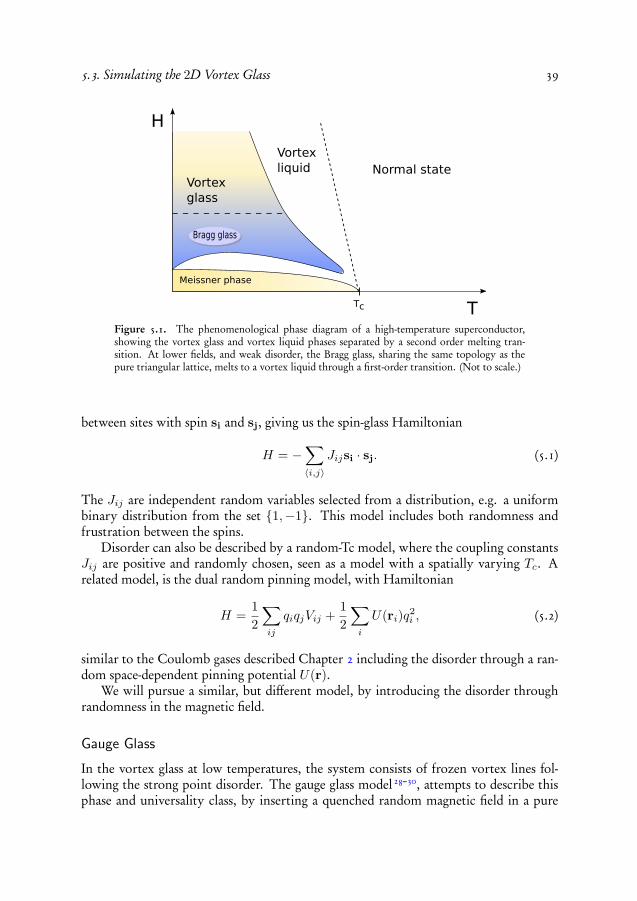
A pure strongly type-II superconductor in the mixed phase with an applied externalmagnetic field has vortices threading the system, forming a triangular Abrikosov vortexlattice. This phase of the pure system is destroyed when an external current is applied

37

38 Chapter 5. Point Disorder

perpendicular to the vortices, since the vortices will feel an applied force making themmove and dissipate energy, and the system ceases to be superconducting.

One way to avoid this forced loss of superconductivity is to pin the vortices, toprevent them from moving, with a pinning force counteracting the generated force fromthe introduction of the current. Such pinning forces naturally arise from defects in thesuperconducting materials, because it is energetically favorable for the vortices to alignthemselves with the disorder. The resulting effect of the disorder on the vortices is anattractive force pinning the vortices to the disorder counteracting the driving force ofapplied currents and thermal fluctuations.

One common type of disorder is point disorder, in which uncorrelated point de-fects within the material pin vortices. Point disorder arises naturally as defects in high-temperature superconductors, e.g. originating from oxygen vacancies or impurities.This type of point defects can artificially be introduced into a clean superconductor,by irradiating samples with electrons and protons

Introducing a weak disorder (low density of defects) into the system will not sub-stantially alter the ordered vortex lattice structure from the pure system at short lengthscales, locally preserving the topology of the triangular lattice symmetry of the system.At longer length scales, though, the interaction of the vortices with the weak disorderwill destroy the lattice symmetry, destroying the long range order and the system en-ters the Bragg glass phase23–25, where the name alludes to the Bragg peaks seen in sucha phase. In this dislocation-free phase the correlation functions for the vortex positionsin the glass, decay according to a power-law. Increasing the temperature, the Bragg glass“lattice” will melt into a vortex liquid through a first-order phase transition.

Increasing the disorder strength, the system enters a new topologically disorderedphase, the vortex glass26,27. This phase is characterized by a vanishing linear resistivity asthe applied current j goes to zero, ρ(j → 0) → 0, indicating that the vortex glass phaseis a true superconducting phase with no linear response to the Lorentz force from theapplied current. This vanishing of the linear resistivity, comes from diverging energybarriers against vortex motion in the vortex glass phase.

The melting transition, when increasing the temperature, from the vortex glass phaseinto a vortex liquid phase occurs through a second order phase transition. This secondorder transition was studied in Paper I, using the gauge glass model as a model for thevortex glass phase.

Figure 5.1 shows some of the main features of a phenomenological phase diagram fora system with uncorrelated point disorder.

5.3 Simulating the 2D Vortex Glass

From the above discussion, we conclude that in order to model the transition from thevortex liquid into the vortex glass phase, disorder must be added to our models. Oneway to introduce disorder is to allow the coupling constants Jij in a spin model to vary

5.3. Simulating the 2D Vortex Glass 39

Figure 5.1. The phenomenological phase diagram of a high-temperature superconductor,showing the vortex glass and vortex liquid phases separated by a second order melting tran-sition. At lower fields, and weak disorder, the Bragg glass, sharing the same topology as thepure triangular lattice, melts to a vortex liquid through a first-order transition. (Not to scale.)

between sites with spin si and sj, giving us the spin-glass Hamiltonian

H = −∑〈i,j〉

Jijsi · sj. (5.1)

The Jij are independent random variables selected from a distribution, e.g. a uniformbinary distribution from the set {1,−1}. This model includes both randomness andfrustration between the spins.

Disorder can also be described by a random-Tc model, where the coupling constantsJij are positive and randomly chosen, seen as a model with a spatially varying Tc. Arelated model, is the dual random pinning model, with Hamiltonian

H =12

∑ij

qiqjVij +12

∑i

U(ri)q2i , (5.2)

similar to the Coulomb gases described Chapter 2 including the disorder through a ran-dom space-dependent pinning potential U(r).

We will pursue a similar, but different model, by introducing the disorder throughrandomness in the magnetic field.

Gauge Glass

In the vortex glass at low temperatures, the system consists of frozen vortex lines fol-lowing the strong point disorder. The gauge glass model28–30, attempts to describe thisphase and universality class, by inserting a quenched random magnetic field in a pure


XY system. Specifically, the disorder is introduced through the magnetic vector poten-tial field A, coupling to the phase of the superconducting order parameter θ, giving theHamiltonian of the gauge glass

H = −J∑〈i,j〉

cos(θi − θj −Aij). (5.3)

Here, J is a positive coupling constant and Aij are quenched random variables takingvalues between −π and π (or 0 and 2π). The random variables Aij are defined on thelinks connecting site i and j and are related to the vector potential of the magnetic fieldB = ∇×A through

Aij =2π

Φ0

∫ j

i

A · dr,

with Φ0 = hc2e the flux quantum. The gauge glass model can be seen as an XY model with

an included quenched (frozen) spatially random magnetic flux in the lattice, affecting thespin interaction. Alternatively, the gauge glass can be viewed as a model for a granularsuperconductor.

Despite the local quenched magnetic fluxes, the gauge glass is, on average, isotropicand with periodic boundary conditions there is no net applied magnetic field. Eventhough the gauge glass is a simple model, there is still no consensus whether there exista finite temperature transition to a glassy phase in 2D31. Paper I, is in part devoted toMonte Carlo simulations and FSS analysis of the equilibrium static properties of the twodimensional gauge glass, finding a scaling consistent with a zero temperature transitionTc = 0.

Dynamics in the Gauge Glass

Using Monte Carlo simulations, we can also study the dynamics of the gauge glass,which will be dependent on the update scheme used. This means that the same staticuniversality class can have many different dynamic universality classes, depending onthe dynamics of the system. Further, the presence of conserved quantities, such as aconserved order parameter, can lead to a different dynamic universality class than theunconstrained system32. In the gauge glass, we are interested in the local relaxationdynamics in the absence of any conserved quantities and therefore we only employ singlespin updates and do not consider any cluster methods. In addition, to observe relaxationsof single spins, the update scheme should not include other global update techniques,such as parallel tempering (c.f. Section 3.5).

At a second order transition, the correlation length diverges ξ ∼ |T−Tc|−ν , meaningthat we will have large correlated fluctuations. It is natural then to assume that thesefluctuations relax back to equilibrium with a correlation time τ that also diverges as weapproach the critical point. This divergence can be expressed as

τ ∼ ξz, (5.4)

5.3. Simulating the 2D Vortex Glass 41

where z is the dynamic critical exponent. In other words, this correlation time measuresthe time it takes for a typical fluctuation to relax.

In order to calculate the dynamic exponent we must study dynamic (time-dependent)quantities such as the resistivity. In our simulations on the gauge glass we calculated theresistivity and time-autocorrelation function of a fake order parameter. Surprisingly, wefind two diverging correlation times, one for the global phase slips and one for the localspins updates.

The correlation time from measuring the time-autocorrelation function probes therelaxation times for the thermally exited spins to relax back to equilibrium. Applyingthe dynamic scaling theory, Eq. (4.25), on this local and time-dependent quantity, thesummed auto-correlation function for systems of different size, collapses onto a singlecurve for the entire time-range. From this collapse we can extract the dependence of τas a function of size giving us the dynamical critical exponent z. In the gauge glass thisdynamic critical exponent was measured to be z = 2.7± 0.2.

A difference between simple scaling collapses in the static and dynamic cases is thatin the latter we have at least two scaling fields, since we include t/τ (c.f. Eq. 4.25). Tosimplify the scaling analysis, it is often better to fix one of the scaling fields in the scalingfunction, and since we are interested in the dynamics, a logical choice would be to fixthe value of L1/ν(T −Tc) for each choice of system size L. This means that each systemsize must be simulated at a different temperature.

There are several other dynamic quantities we can study, two of which are the con-ductivity and resistance. Naively, one would expect all dynamic quantities to yieldthe same dynamical exponent, measuring the characteristic thermal fluctuations of thephases. However, in the gauge glass model, measuring the resistance from the fluctu-ations of the phase boundary (cf. Eqs. (4.33) and (4.35)), reveals a slightly differentdynamic behavior than obtained from the time-autocorrelation function above.

Assuming the same dynamic critical exponent as previously, the resulting collapse ofthe time-dependent resistance only occurs in a medium time-range interval. For longertimes, though, the scaling does not work, indicating that there might be a second diverg-ing correlation time. Since the resistance measures vortex motion through the system,it is natural to associate this longer correlation time with the vortex motion. Measuringthe resistance, therefore, captures these global events of voltage fluctuations described bya different dynamic critical exponent. The resistance at large times could be describedby an activated Arrhenius form,

R ∼ e−V/T , (5.5)

where V is an effective energy barrier height, separating two local minima in the roughenergy landscape, that vortices need to surmount in order to cross the system. Thisenergy barrier is assumed to scale with system size as V ∼ Lψ.

Figure 5.2 shows the resulting 2π phase twist, when a vortex is allowed to wanderthrough a system with periodic boundary conditions. Using fluctuating boundary con-ditions instead, allows the system to unwind this twist, from which a voltage in theperpendicular direction can be measured.


Figure 5.2. The XY model with periodic boundary conditions, in which a vortex and anti-vortex pair separate (top to bottom). As the vortex passes through the system a phase twistemerges in the direction perpendicular to the motion of the vortex due to the periodic bound-ary conditions.

Chapter 6

Correlated Disorder

The introduction of disorder into pure systems can substantially alter the differentphases and specifically the second order phase transitions between phases. In the pre-vious chapter, strong point disorder changed the ordered Abrikosov vortex lattice ofhigh-temperature superconductors into a glassy phase called the vortex glass. In thischapter we study the effects of disorder further, specifically when the disorder is corre-lated.

6.1 Harris Criteria

The presence of weak disorder in a system changes the critical temperature from thepure system’s Tc to the disordered system’s Tc, but the existence of disorder does notnecessarily lead to a change in the system’s universality class for the transition. There isa heuristic argument by Harris33, setting a condition for when the disorder is a relevantvariable, destabilizing a pure system’s fixed point.

Disorder, as included in some of the models discussed in the current chapter, is in-troduced by altering the coupling constants J and can equivalently be seen as a systemwith a spatial variation in the transition temperature. Therefore, we introduce a spatiallyvarying critical temperature Tc(r) and study the variations of this critical temperaturefrom the overall global critical temperature Tc of the disordered system,

δTc(r) ≡ Tc(r)− Tc. (6.1)

In addition, we also define a correlation volume Vξ for the continuous transition fromthe scaling behavior of the correlation length ξ ∼ |T − Tc|−ν as T → Tc.

The argument is as follows: If the fixed point associated with the pure system isto survive the introduction of disorder, the average of the fluctuations δTc(r) over acorrelation volume Vξ = ξd, must have a disorder root-mean-square fluctuation that issmall compared to |T −Tc| ∼ ξ−1/ν as T → Tc. Otherwise, the disorder will destabilizethe pure fixed point and the system will change universality class with new fixed points.

43

44 Chapter 6. Correlated Disorder

The disorder root-mean-squared fluctuations averaged over a correlation volume are

⟨(∫Vξ

ddrVξ

δTc(r)

)2⟩1/2

dis.

=

[∫Vξ

ddrVξ

∫Vξ

ddr′

Vξ〈δTc(r)δTc(r′)〉dis.

]1/2

. (6.2)

To find the dependence of the above expression, in terms of the correlation length ξ,begin by studying the correlation function in the right hand side. The correlation func-tion of the fluctuations in the critical temperature 〈δTc(r)δTc(r′)〉dis., can be expressedas the correlation function of the coupling constants 〈J(r)J(r′)〉 and, likewise, of thedisorder. In the simplest case, the disorder is completely uncorrelated and the correla-tion function is therefore a delta function δd(r − r′). In this case, Eq. (6.2) evaluates toV−1/2ξ = ξ−d/2 ∼ |T − Tc|dν/2. Now, comparing this with the requirement that in

order for the transition to be self-consistent, this expression has to be much smaller than|T − Tc| as T → Tc, leads to the condition dν/2 > 1.

Three relatively simple cases for the disorder are: (a) uncorrelated disorder, (b) fullycorrelated disorder in one direction and uncorrelated in the rest, and (c) long-range cor-related disorder obeying a power-law34. The uncorrelated disorder case, with a deltafunction correlation, was discussed above, resulting in the condition ν > 2/d. Inthe case with disorder fully correlated in one direction and the remaining directionsuncorrelated, the correlation function is δd−1(r − r′) and the condition changes intoν > 2/(d − 1). Finally, for the long-range power-law correlated disorder g(r) ∼ r−ζ

(with d > ζ), the condition for the stability of the pure fixed point is ν > 2/ζ.In summary, Harris33 showed that for a continuous transition, uncorrelated weak

disorder is irrelevant if the pure system obeys ν > 2/d. The generalization by Weinriband Halperin34 to the case of power-law correlated disorder, with correlation functiong(r) ∼ r−ζ as r →∞, tells us that disorder is irrelevant if

dν − 2 > 0 if ζ ≥ d (Harris) (6.3)ζν − 2 > 0 if ζ < d, (6.4)

representing the short- and long-range correlated regimes respectively.

6.2 Helium-4 Confined in Aerogel

According to the Harris criterion33, introducing weak random point disorder into a 4Hesystem should not change the universality class from the pure system, since ν ≈ 0.67 inthe pure system15. If we instead introduce correlated disorder, the system could changecritical behavior described by a new universality class with different exponents. In thissection, we study the superfluid λ-transition of 4He, where disorder is inserted thoughthe use of the aerogel material.

6.2. Helium-4 Confined in Aerogel 45

Aerogel

Aerogel is an extremely porous solid, making it an interesting material to use, specifi-cally when special requirements are to be met, such as in space missions. Holding thetitle World’s Lightest Solid35,36, aerogel samples can have porosities up to 99.9%, whichmakes aerogel practically as light as air. Due to its high porosity, aerogel has successfullybeen used in space missions, such as the Stardust mission37, where rapidly moving dustgrains blown off the comet Wild 2 were collected in an aerogel array acting as an effectivecushion safely trapping the rapid particles for later examination. Aerogel is also a verygood thermal insulator, which together with its low density makes it attractive in spacemissions.

The aerogel structure consists of silicon dioxide particles forming strands of a fewnanometers in size, which are inter-connected, creating a very porous structure withcavities ranging up to 200 nm in size38. In addition, the aerogel structure forms a fractalon a length scale range from a few nanometers up to a hundred nanometers39.

The porous and fractal nature of the aerogel structure enables studies of disorder in4He. Experiments38,40, with liquid helium in aerogel, indicate a new universality classfor the superfluid transition and also a surprising violation of the Josephson hyperscalingrelation α = 2 − dν. In Paper II, we study this problem numerically, by simulating anXY model in the presence of disorder in the form of an aerogel-like cluster structure.

DLCA Clusters

The correlated impurities represented by the aerogel structure can in simulations bemodeled by the Diffusion Limited Cluster Aggregation (DLCA) algorithm41,42. Thisalgorithm tries to mimic the diffusion of the particles in the aerogel structure whenthey are initially forming aerogel in its gel state. The resulting structure shows fractalproperties with a fractal dimension of df ≈ 1.8.

The algorithm starts by choosing the desired density of aerogel particles and dis-tributes them randomly within the simulation volume. The particles will then diffusefollowing a Brownian motion and each time two of them collide they stick irreversiblytogether, forming a larger cluster. This new cluster can also diffuse, generating largerand larger clusters until one single cluster remains.

Assuming the Brownian diffusion is described by the Einstein-Stokes equation withdominating viscous forces, the diffusion constant D is inversely proportional to theviscosity η and radius r of the spherical particle undergoing the diffusion,

D =kBT

6πηr. (6.5)

The fractal structures or clusters we are building will have a mass m proportional to itssize r to the power of the fractal dimension df ,

m ∼ rdf . (6.6)

This relation gives us the dependence of the size of the cluster on its mass, r ∼ m1/df .Consequently, the dependence of the diffusion constant for the fractal cluster on the


mass m of the fractal isD(m) ∼ 1

r∼ m−1/df . (6.7)

The probability pi to select cluster i with mass mi to diffuse in the next update step isproportional to the diffusion constant of that cluster D(mi). This can be encoded intothe dynamics of the algorithm by choosing the cluster selection probability to be

pi =m−αi∑

i m−αi

, (6.8)

where α = 1/df . This selected cluster is then randomly moved one lattice spacing alongany direction, merging together with any other clusters it has contact with along theway. A numerical study of the generated DLCA clusters, with different choices on theparameter α, shows that the generated structures all have the same fractal dimension,irrespective of the choice of α.

The choice of dynamics, Brownian motion of diffusing particles in a viscous solu-tion, generates one single cluster with a fractal dimension, in some length scale interval1,equal to df ≈ 1.8. This fractal dimension is very similar to the fractal dimension seenin certain aerogels (base-catalyzed). An example of such a generated DLCA cluster isshown in Fig. 6.1.

Harris Criterion

The isotropic fractal structure of the DLCA cluster, with a fractal dimension df ≈ 1.8,enables us to express the density-density correlation function as a function of distance43

c(r) =1Vf

∑r′

ρ(r + r′)ρ(r′), (6.9)

where ρ(r) is a local density, equal to one if a site is part of the fractal cluster and zerootherwise, and Vf is the total number of particles in the cluster. Since fractals are scaleinvariant, the density-density correlation function has the property2 c(r) ∼ r−ζ , withζ = d− df ≈ 1.2 for the DLCA cluster in three dimensions.

A naïve application of the generalized Harris criterion presented in section 6.1 leadsto the conclusion that the disorder is relevant, since for the pure system ν ≈ 0.67, andthe condition for weak disorder to be irrelevant (c.f. Eq. (6.4)) reads

ζν − 2 > 0, for ζ < d. (6.10)

On the other hand, at longer length scales, the disorder in the DLCA cluster changesfrom being fractal to uncorrelated, since the density of the cluster is initially chosen to afixed value. In this case, one would expect the pure fixed point to be barely stable, since

1The physical object cannot be fractal on all length scales, since the aerogel density is initially fixed.2The density-density correlation function for a fractal is a homogeneous function 43 c(br) = b−ζc(r),

with 0 < ζ < d

6.2. Helium-4 Confined in Aerogel 47

Figure 6.1. A diffusion limited cluster-cluster aggregation realization, used to model the aero-gel system in numerical simulations.

now ν > 2/d = 2/3 is valid. A way to avoid the Harris criterion is to note that thedisorder, introduced by the DLCA cluster, is strong, therefore the implications of theHarris criterion need not be true. In Paper II we find new critical exponents for the 3DXY model with disorder described by a DLCA cluster, indicating a different universalityclass for this system, but we also note that a slow crossover to the pure 3D XY modelsuniversality class can not be ruled out.

Modeling Helium-4

The universality class of 4He at the λ-transition is believed to be the same as that of thephase transition in the pure 3D XY model,

H = −∑〈ij〉

Jij cos(θi − θj), (6.11)

where θi denotes the phase of the complex order parameter Ψ = |Ψ|eiθ. In the pure 3DXY model, the coupling constants Jij are all set to a constant positive value, often J = 1,since other constant values can be transformed to the J = 1 case with a redefinition ofthe temperature −βH[J ] = −(βJ)H[J = 1].


In order to simulate helium-4 in the presence of the aerogel disorder, we must intro-duce disorder into the the pure XY model. The DLCA cluster, representing aerogel, willexclude sites that are occupied by helium in the pure case. It is then natural to make thechoice that the coupling constants Jij are equal to one only between helium sites andzero if at least one of the sites i or j is part of the DLCA cluster. This quenched disorderis then held fixed throughout the simulation.

6.3 Vortex ModelThe Meissner phase in superconductors is characterized by the expulsion of magneticfields within the superconductor. The transition into the mixed state of type-II su-perconductors allows magnetic fields to penetrate the system, channeled through thevortices. Introducing linearly correlated defects, such as columns, vortices will find itenergetically favorable to align themselves on top of such defects, extending along thedirection of the disorder and thereby introducing a reluctance towards deviations fromthese defects. By applying a second, weaker, field perpendicular to the columns, a tran-sition from an phase in which no magnetic field penetrates in the transverse directionto a phase in which the field has a component in this direction can be seen. This is thetransverse Meissner transition (TMT).

Columnar Disorder and the Bose Glass

Correlated defects in a type-II superconductor can be introduced by heavy-ion irradi-ation of samples, producing tracks of damaged material forming the disorder. In thepresence of such columnar disorder, applying a magnetic field at low enough tempera-tures, the thermal energy is weak and the vortices find it energetically favorable to betrapped onto the columnar defects, forming a new glassy state called the Bose glass44,45

(related to the glassy phase of 2D bosons with point disorder46). From the Bose glassphase, raising the temperature, the stable Bose glass phase melts through a second-ordertransition into an entangled vortex liquid. Figure 6.2 shows the phase diagram of ahigh-temperature superconductor in the presence of correlated disorder47.

The Transverse Meissner Transition

Many systems are isotropic at large length scales, where anisotropies at shorter scalesdisappear and systems show a high degree of symmetry. The breaking of these sym-metries in a system will often transfer the system from one universality class into an-other. A typical symmetry breaking disorder introduced in superconductors are cor-related columnar defects, extending from microscopic to macroscopic scales. Since thecorrelation length near a second order phase transition diverges, a situation where thesystem shows two different diverging correlation lengths, parallel and perpendicular tothe symmetry breaking columnar defects, can emerge. This symmetry breaking can betaken one step further by breaking the in-plane symmetry in the directions perpendic-

6.3. Vortex Model 49

Figure 6.2. The phase diagram of a high-temperature superconductor with correlated disorder,showing the Bose glass phase at low temperatures. In this glassy phase, vortices are perturbedfrom their triangular lattice sites in the pure system, in a way that locally the Bose glass vortexglass retains the topology of the pure system, but at larger distances the disorder destroys thelong range translational order of the Abrikosov lattice. The thin white lite is the melting curveof the pure system. (Figure is not to scale.).

ular to the columns. The symmetry is removed by applying an external magnetic fieldat an angle with the columns. The result of this asymmetric setup can lead to diverg-ing correlation lengths at a continuous transition, with exponents that differ in all threedirections.

In the transverse Meissner transition, briefly discussed above, one introduces corre-lated defects, such as columnar defects, and then looks at the transition when a field isapplied. If the field is parallel to the correlated defects, we can measure the so calledBose glass transition. Now slowly rotating the external field away from the defects,the vortices will, at small angles, still localize along the columnar defects, even thoughthere is a non-zero transverse applied field in this case. As the perpendicular magneticfield increases there will finally be a transition into a a state when the vortex flux linesdecouple from the columns producing a transverse flux within the superconductor. Fig-ure 6.3 illustrates this transition, from a zero transverse flux B = 0 into a finite fluxB 6= 0 along a direction perpendicular to the columns. This transition is the transverseMeissner transition.

The lack of symmetry in the transverse Meissner transition along the three spatialdirections makes it interesting to study if such systems change their universality classinto one where correlation lengths along each direction diverge with different exponents,when approaching the transition.


Figure 6.3. The transverse Meissner transition in high-temperature superconductors withcolumnar disorder and a strong field H‖ parallel to the columns. For a weak magnetic trans-verse field H⊥ (left), the vortex lines are pinned to a single column. Increasing the transversefield (right), the vortices start to follow the applied field direction, producing a finite magneticflux in the transverse direction destroying the transverse “Meissner” phase.

Anisotropic Scaling

There is an interesting analytical scaling result48 for the Transverse Meissner transition,showing that the ratios of the exponents for the diverging correlation lengths in thethree different spacial directions are 1,2 and 3! Here, I will give an quick derivation ofthis 1-2-3 scaling result.

First, assume we have a system extending in three spatial directions with the corre-lated disorder, the columns, along the z direction. Apply a magnetic field H at an angleto the disorder, such that there is a strong component H‖ parallel to the disorder (alongz) and a weak component H⊥ perpendicular to the disorder along the x direction. Theassumption is that we will have a different correlation length scaling exponent in each ofthe three spatial directions,

ξy = ξ ∼ |T − Tc|−ν (6.12)ξx = ξχ (6.13)ξz = ξζ . (6.14)

In such a system, the scaling of the disorder-averaged free energy density f , is assumedto follow

f(T,Hx,Hy,Hz) = l−(χ+1+ζ)f(l1/ν(T − TTM ), lχHx, lHy, lζHz) (6.15)

where l is a length scale factor and TTM is the transverse Meissner phase transition tem-perature. The temperature scaling variable is defined in the usual way, while the scalingof the magnetic variables as the inverse length, Hi ∼ l−1

i , follows from the energy den-sity B ·H ∼ l−(χ+1+ζ) together with the scaling form of Bi = −∂f/∂Hi = (∇×A)i ∼l−(χ+1+ζ)/l−1

i . The scaling of the magnetic induction Bi, follows, in turn, from the scal-ing of the vector potential Ai ∼ l−1

i by the way it enters into the free energy, scaling like

6.3. Vortex Model 51

∇i ∼ l−1i . Finally, the magnetic permeability scales as µi = ∂Bi/∂Hi ∼ l−(χ+1+ζ)/l−2

i .In summary, the scaling relations for the magnetic induction and permeability are

Bx ∼ l−(1+ζ) , µx ∼ lχ−1−ζ (6.16)By ∼ l−(χ+ζ) , µy ∼ l1−χ−ζ (6.17)

Bz ∼ l−(χ+1) , µz ∼ lζ−χ−1. (6.18)

Arguing that the magnetic permeability along the z direction does not diverge at thetransition46, µz ∼ l0, gives us the condition,

ζ − χ− 1 = 0. (6.19)

We now only need one more constraint to fix the exponents.To derive the correlation length exponents, Eqs. (6.12) - (6.14), for the different direc-

tions, we continue by studying the scaling relation for the free energy density, Eq. (6.15),when we apply a small rotation to the system. We first observe that the disorder-averagedfree energy density is rotationally invariant in the plane perpendicular to the columnardisorder, meaning that the free energy density should remain invariant after applying ainfinitesimal rotation ϕ on the perpendicular component of the magnetic field H⊥,

Hx = H⊥ → H′

x = H⊥ cos ϕ = H⊥(1− 12ϕ2) + O(ϕ4) (6.20)

Hy = 0 → H′

y = H⊥ sinϕ = H⊥ϕ + O(ϕ3). (6.21)

Application of this rotation should leave the free energy invariant,

δf = f(t, H′

x,H′

y,Hz)− f(t, Hx, 0,Hz) (6.22)

= −H⊥ϕ2

2∂f

∂Hx+ H⊥ϕ

∂f

∂Hy+

H2⊥ϕ2

2∂2f

∂H2y

+ O(ϕ3), (6.23)

meaning that each order in ϕ should vanish. Setting the coefficients of each order in ϕto zero results in the following two requirements,

By = 0 (6.24)Bx = µyH⊥, (6.25)

from which χ = 2 can be obtained (c.f. Eqs. (6.16) and (6.17)). Together with theprevious result Eq. (6.19) we conclude that ζ = 3.

Experimentally, it may be difficult to study the transverse Meissner transition, dueto the fact that the transition occurs when the tilt angle of the applied field away fromthe columns is very small (order of a few degrees). Despite this, in Paper III a continuoustransition from a solid, with vanishing resistivity, to a vortex liquid, with finite resistiv-ity, was observed at larger tilt angles. The subsequent analysis showed that in the tiltangle range θ = 15◦−65◦ the correlation lengths at the solid-to-liquid transition divergewith three different exponents, which are close to the 1-2-3 result of the TMT transition,even though the precise values could not be verified from the available data.

Chapter 7

Logarithmic Gas

The two dimensional Coulomb gas, related to the 2D XY model through a duality trans-formation, shows an interesting type of transition, named the Berezinskii-Kosterlitz-Thouless49–51 (KT) transition, whose origin is the unbinding of topological defects (vor-tices). In three dimensions, the Coulomb gas, with an interaction depending inverselyon the distance between particles, is known not to have a transition at any finite temper-ature. The charges in this system are always unbound forming a plasma phase for anyT > 0. The question then arises if we can modify the interaction potential and producea KT-like transition in three dimensions. This interesting scenario has recently beensuggested52,53 in a three dimensional system, where the interaction potential betweenparticles is assumed to be logarithmic.

7.1 Kosterlitz-Thouless Transition

Mermin-Wagner theorem

According to a theorem by Mermin and Wagner54, two dimensional systems with ashort-ranged interaction and a continuous symmetry, can not have any long range order.We can show this lack of long-range order for the 2D XY model, using a simplifiedargument for the fluctuations of the phase field.

Start by making the assumption that the system does have a transition into an or-dered state below some temperature, in which the phase field θ(r) can be written as

θ(r) = θ0 + δθ(r), (7.1)

where θ0 is the uniform order parameter field minimizing the energy H and δθ(r) arethe displacements from this direction. We are interested in the mean-square value ofthese phase fluctuations 〈(δθ(r))2〉 in the low temperature phase, where we expect themto be small and finite and thus not destroy the ordered state. Given the fluctuations, we

53

54 Chapter 7. Logarithmic Gas

express the energy of the system relative to the assumed ordered state (c.f. Eq. (2.9))

∆H =∫

d2r12|∇δθ(r)|2, (7.2)

resulting in the partition function Z =∫Dδθ e−β∆H taking a Gaussian form. The

correlation function 〈(δθ(r))2〉 can therefore be expressed as1

〈(δθ(r))2〉 =∫ Λ

0

d2k(2π)2

1k2

, (7.3)

where Λ is some cutoff, which we can relate to our lattice constant. From this we seethat in two dimensions, the mean-square of the fluctuations diverges logarithmically andis not bounded and small as we assumed.

This means that the 2D XY model, and consequently the Villain model and 2DCoulomb gas, do not have any finite transition temperature to an ordered phase withlong-range correlations. Still, there are other, interesting, possibilities for a phase transi-tion in these systems.

Topological excitations

Even though the 2D XY model lacks any broken symmetry phase with long-range cor-relations, doing a low temperature expansion, the spin-waves (i.e. long wave-lengthexcitations) show correlations that slowly decay following a power law, referred to asquasi-long-range order. Conversely, a high-temperature expansion of the 2D XY model,instead shows the expected exponential decay of correlations with distance. The naturalquestion is what causes the change in the correlation function from a power-law decay toan exponential decay? The answer to this is the existence of topological defects (vortices)that, when present, can destroy the quasi-long-range order. On the other hand, pairs ofvortices with opposite vorticity can, at low enough temperatures, bind, leading only toa local disturbance of the phase field, enabling the quasi-long range order to prevail. Thephase transition in the 2D XY model is, therefore, governed by the unbinding of vortexpairs and the subsequent proliferation of free vortices in the system.

Energy-Entropy Argument

Despite the Mermin-Wagner theorem, the 2D Coulomb gas model and likewise the 2DXY model, shows a finite temperature transition governed by the proliferation of chargesand vortices respectively. The existence of this transition is most readily seen if onestudies an energy-entropy argument for the free energy increase when inserting a charge(or vortex in the XY systems).

1To do the Gaussian integral giving the correlation function, insert into the Hamiltonian, a source fieldJ(r) coupling to the order parameter and then take two functional derivatives with respect to J(r). Alsoworking in Fourier space decouples the Fourier components into separate integrals 55.

7.2. Logarithmic Gas in 3D 55

At any chosen temperature, the free energy expresses a competition between energyand entropy,

F = U − TS. (7.4)

The entropy of inserting a single charge (or vortex) in a two dimensional system of sizeL, with a lower cutoff a2, can be calculated by observing that the number of distinctpositions available to place a charge is (L/a)2, giving the entropy of a single charge

S = kB ln(L/a)2. (7.5)

The self-energy of a single charge in a system of size L, assuming we have a linearisotropic dielectric medium with dielectric constant ε is

H0 =12ε

V (0) =12ε

∫ 2π/a

2π/L

d2k

(2π)2Vk =

{Vk =

2π

k2

}=

12ε

lnL

a(7.6)

where Vk is the Fourier transform of the Coulomb potential and a is the lower cut-off ofa system of size L2. This self-energy diverges at long length scales, becoming infinite foran infinite system. The free energy change of inserting a single charge into the system isthen

∆F =(

12ε− 2kBT

)ln

L

a. (7.7)

From this expression we can deduce that for temperatures T < (4ε)−1 (set kB = 1)there is an increase in the free energy for inserting a single charge to the system, but fortemperatures T > (4ε)−1 this is no longer the case and we will have charge proliferation.In the vortex picture, these free charges will destroy any quasi-long-range order in thesystem.

The argument above, can be modified to accommodate the existence of two particles,with opposite charge, bound together. Calculating the energy of such a pair shows thatit is finite for an infinite system, and thus any such excitations will always be present atany finite temperature. It is when these pairs unbind, that we get charge proliferationand a phase transition occurs. In addition, these dipole pairs give rise to the screeningeffect effectively captured by the dielectric constant ε.

7.2 Logarithmic Gas in 3DAs was shown in connection to the XY model in Eq. (2.11), the dual model of the2D XY model is the 2DCG, where the vortices are represented by charged particlesof integer charge, corresponding to the vorticity. In this two dimensional system theparticles interact according to a logarithmic interaction, which is the solution to thePoisson equation,

∇2V (r) = −2πδ(r) (7.8)

2In our numerical simulations this is always set equal to the lattice spacing, which, in turn, is set to unity.


In three dimensions, the Coulomb gas charges interact according to the well knownpotential, inversely proportional to distance, which is the fundamental solution to

∇2V (r) = −4πδ(r). (7.9)

This model is known6 not to have any finite temperature transition into a state wherethe particles are bound in charge pairs; a conclusion which can also be drawn from asimilar energy-entropy balance argument given above. In the three dimensional case,the self-energy, Eq. (7.6), is inversely proportional to distance r−1, while the entropyremains proportional to the logarithm of r. Both these terms enter as negative termsin the free energy change Eq. (7.4), indicating that it is always energetically favorable toinsert free vortices.

Changing the interaction above for the three dimensional system, into an interactionwhose long range form is logarithmic,

V (r) ∼ − ln(r), (7.10)

might lead to a change in the phase transition, from a zero temperature transition intoa finite one. It has been suggested52,53 that the new phase transition is of the Kosterlitz-Thouless type, since by construction, it shares many properties of the Hamiltonianwith the 2D Coulomb gas. Recently, this scenario has been investigated in Monte Carlosimulations56,57, with results supporting the existence of a KT phase.

The logarithmic interaction between charged particles in three dimensional classicalsystems has also been suggested as a model for compact gauge theories coupled to matterfields. Here, instead, we concentrate on the properties of the actual model and will notdiscuss the validity of this model as a model for gauge theories.

Naively, performing the same argument for the energy and entropy contributionto the logarithmically interacting gas, we find that since we are in a three dimensionalspace, the contribution from the number of positions available to a charge increases to(L/a)3. Thus, the free energy increase for inserting one charge in the system is

∆F =(

12ε− 3kBT

)ln

L

a, (7.11)

which suggests that a transition should exist for εTc = 1/6.

Polarization free system

In Coulomb gas models, there is a requirement on the overall charge of the system,imposing charge neutrality, due to the divergence of the Hamiltonian when the totalcharge does not vanish. Similarly, the logarithmic gas shares this requirement and inaddition also demands that there be no net polarizability in the system.

In Monte Carlo simulations, the charge neutral restriction can be obeyed by be-ginning with an initial charge neutral configuration and only allowing update schemeswhich preserve the overall charge. One examples of such an update scheme is the trial

7.2. Logarithmic Gas in 3D 57

Figure 7.1. Warmup time comparison between a double dipole update scheme comparedto a scheme where single dipoles are used together with configuration space restriction andsampling only at polarization free configurations. The restricted single dipole scheme is moreefficient, reaching equilibrium faster. Data taken from a system of size L = 8 and temperatureT = 0.225.

move of inserting one dipole pair. This, however, alters the polarizability of the system,making it unsuitable for simulating the logarithmically interacting particle gas. Instead,generalizing the update scheme to one where two dipoles with opposite directions areinserted, will lead to configuration with an unaltered total charge and total polarization.

However, the update algorithm of inserting two dipoles is very slow. A faster methodis to update with single dipoles, allowing for polarization fluctuations, but instead onlytake measurements when the overall polarization of the system vanishes. One problemwith this method is that there is a large probability that the system explores configura-tions far from the polarization free system. In order to keep the system close to zeropolarization we can insert a hard cutoff for polarizations with magnitude larger thanone, i.e. we never accept trial updates resulting in a system whose total polarization istwo. This restricted sampling method, turns out to give the correct sampling, and is anexcellent compromise between allowing polarization fluctuations and measuring only atzero polarization. Figure 7.1 shows that the restricted sampling method is much moreeffective than the two dipole update method, enabling us to reach larger system sizes insimulations.

Scaling

The main idea in our scaling ansatz used to study the transition for the logarithmic gasis to attempt a similar scaling analysis as was performed for the 2D gauge glass in Paper I,in which Tc = 0. One quantity we can measure in particle gas models is the dielectric


constant, related to the helicity modulus of the XY models. The dielectric constant canbe calculated form the expression

ε−1 = limk→0

[1− Vk

LdT〈|qk|2〉

], (7.12)

where Vk is the Fourier transform of the logarithmic interaction potential and qk isrelated to the density of particles at wave vector k.

The scaling behavior of the dielectric constant, can be analyzed by doing a finite sizescaling collapse from simulation data of different system sizes L,

ε−1(T,L) = ε−1(L1/ν(T − Tc)). (7.13)

The analysis seems to indicate that the best choice resulting in a collapse of curves ofdifferent L is with a choice of Tc = 0, indicating that the logarithmic gas in threedimensions does not have a transition at any finite temperature.

Concluding, further analysis of the logarithmically interacting particle gas model isneeded in order to settle the question whether there exist any phase transition at a finitecritical temperature or if the model has only a zero temperature transition. While somerenormalization group studies52,53 show the existence of a finite temperature transition,other work58,59 has suggested that in a three dimensional system with logarithmic inter-actions, a 1/r Coulomb interaction term will be generated and this will dominate thelarge system behavior, always leaving the system in a plasma phase. Our current MonteCarlo simulation results give a first indication consistent with the lack of a transition forany T > 0.

Acknowledgments

During my many years at the theoretical physics department at KTH, I have come toknow many people. Before you start reading this acknowledgment in search of yourname, I want to point out that, statistically, I will surely forget to thank some of you.Therefore, I begin by thanking all you nameless heroes that have made this possible,thank you! On the other hand, some people have made such a lasting impression, that Iactually do remember them and would like to devote some paragraphs to thank them inparticular.

First and foremost, I thank my main supervisor, Professor Mats Wallin, for invitingme to join his group and research area of statistical physics. You have countless timesexplained and enlightened me in the field of physics.

During the later part of my studies, I have come to enjoy discussions with Dr. JackLidmar, always there and always taking time to answer, think and ponder any questionI had. Your advice has been most valuable.

Since my research mainly focused on numerical and theoretical aspects of physics, Iwas glad that there were people knowledgeable in the experimental aspects of my field.The experimental group at KTH in Kista, with Magnus Andersson and Beatriz Espinosa-Arronte, did the real thing, applying their craft of meticulously preparing and measuringsamples. Even though the collaboration was short it has contributed to my knowledgeof high temperature superconductors.

Four PhD students, current and past, have contributed to make my stay at the de-partment really enjoyable. Martin Lindén, my ever present roomie, whose biologicallyinclined research I sometimes envy. Sara Bergkvist, who just beat me to a PhD degree,Anders Biltmo, I bid you Godspeed and a former PhD student Anders Vestergren. I havecertainly enjoyed all your company and discussions during our espresso breaks, on ev-erything, including trumpets, ice-skating, films and tanks.

Further, I have also enjoyed several conversations with many people at the depart-ment, especially the people of house 13 in the group of Professor Anders Rosengren.Thank you for this memorable time Anders Rosengren, Per-Håkan Lundow and PatrikHenelius.

A special thank you is also directed to my truly good friend Rickard Armiento. Ifondly remember the good years when he was a PhD student at the same department.

Also, a big thank you to my parents, who despite having a hard time understanding

59

60 Acknowledgments

my research topic — whenever I dared venture into explaining it — have always sup-ported me. Specifically, I found the regular, exceptionally delicious, home-made Greekfood-catering I received during the writing of this thesis very practical.

Finally, I want to acknowledge generous funding from the Göran Gustafsson Foun-dation, without whose support this thesis would simply not exist.

Marios Nikolaou,Stockholm, 27 Feb 2007

Bibliography

[1] J. Bardeen, L. N. Cooper, and J. R. Schrieffer, Phys. Rev. 108, 1175 (1957).

[2] V. L. Ginzburg and L. D. Landau, Sov. Phys. JETP 20, 1064 (1950).

[3] L. P. Gorkov, Sov. Phys. JETP 9, 1364 (1959).

[4] J. Villain., Journal de Physique 36, 581 (1975).

[5] J. V. José, L. P. Kadanoff, S. Kirkpatrick, and D. R. Nelson, Phys. Rev. B 16, 1217(1977).

[6] A. M. Polyakov, Nucl. Phys. B 120, 429 (1977).

[7] N. Metropolis, A. W. Rosenbluth, M. N. Rosenbluth, A. M. Teller, and E. Teller,J. Chem. Phys. 21, 1087 (1953).

[8] M. E. J. Newman and G. T. Barkema, Monte Carlo Methods in Statistical Physics(Oxford University Press, 1999).

[9] U. Wolff, Phys. Rev. Lett. 62, 361 (1989).

[10] K. Hukushima and K. Nemoto, J. Phys. Soc. Jpn. 65, 1604 (1996).

[11] M. C. Tesi, E. J. Janse van Rensburg, E. Orlandini, and S. G. Whittington, J. Stat.Phys. 82, 155 (1996).

[12] A. M. Ferrenberg and R. H. Swendsen, Phys. Rev. Lett. 61, 2635 (1988).

[13] A. M. Ferrenberg and R. H. Swendsen, Phys. Rev. Lett. 63, 1195 (1989).

[14] H. E. Stanley, Rev. Mod. Phys. 71, S358 (1999).

[15] M. Campostrini, M. Hasenbusch, A. Pelissetto, and E. Vicari, Phys. Rev. B 74,144506 (2006).

[16] J. D. Reger, T. A. Tokuyasu, A. P. Young, and M. P. A. Fisher, Phys. Rev. B 44,7147 (1991).

61

62 Bibliography

[17] M. E. Fisher, M. N. Barber, and D. Jasnow, Phys. Rev. A 8, 1111 (1973).

[18] P. Olsson, Phys. Rev. B 72, 144525 (2005).

[19] K. Binder, Z. Phys. B 43, 119 (1981).

[20] K. S. D. Beach, L. Wang, and A. W. Sandvik, cond-mat/0505194 (2005(unpub-lished)).

[21] H. Weber and P. Minnhagen, Phys. Rev. B 37, 5986 (1988).

[22] W. P. Beyermann, N. L. Huang-Liu, and D. E. MacLaughlin, eds., Random Mag-netism, High-Temperature Superconductivity (World Scientific, Singapore, 1994), p.113.

[23] T. Giamarchi and P. Le Doussal, Phys. Rev. B 52, 1242 (1995).

[24] T. Giamarchi and P. Le Doussal, Phys. Rev. B 55, 6577 (1997).

[25] T. Klein, I. Joumard, S. Blanchard, J. Marcus, R. Cubitt, T. Giamarchi, andP. Le Doussal, Nature 413, 404 (2001).

[26] M. P. A. Fisher, Phys. Rev. Lett. 62, 1415 (1989).

[27] D. S. Fisher, M. P. A. Fisher, and D. A. Huse, Phys. Rev. B 43, 130 (1991).

[28] G. Blatter, M. V. Feigel’man, V. B. Geshkenbein, A. I. Larkin, and V. M. Vinokur,Rev. Mod. Phys. 66, 1125 (1994).

[29] W. Y. Shih, C. Ebner, and D. Stroud, Phys. Rev. B 30, 134 (1984).

[30] D. A. Huse and H. S. Seung, Phys. Rev. B 42, 1059 (1990).

[31] J. Um, B. J. Kim, P. Minnhagen, M. Y. Choi, and S.-I. Lee, Phys. Rev. B 74, 094516(2006).

[32] P. C. Hohenberg and B. I. Halperin, Rev. Mod. Phys. 49, 435 (1977).

[33] A. B. Harris, J. Phys. C 7, 1671 (1974).

[34] A. Weinrib and B. I. Halperin, Phys. Rev. B 27, 413 (1983).

[35] C. Folkard, ed., Guinness World Records 2005 (Bantam Dell, 2005).

[36] NASA, Guinness world records certificate (2007), http://stardust.jpl.nasa.gov/images/guinnesscert.jpg [Online; accessed 22-January-2007].

[37] D. Brownlee, P. Tsou, J. Aleon, C. M. O. Alexander, T. Araki, S. Bajt, G. A.Baratta, R. Bastien, P. Bland, Phil an d Bleuet, J. Borg, et al., Science 314, 1711(2006).

http://stardust.jpl.nasa.gov/images/guinnesscert.jpg

http://stardust.jpl.nasa.gov/images/guinnesscert.jpg

63

[38] J. Yoon, D. Sergatskov, J. Ma, N. Mulders, and M. H. W. Chan, Phys. Rev. Lett.80, 1461 (1998).

[39] M. Chan, N. Mulders, and J. Reppy, Physics Today 49, 30 (1996).

[40] M. H. W. Chan, K. I. Blum, S. Q. Murphy, G. K. S. Wong, and J. D. Reppy, Phys.Rev. Lett. 61, 1950 (1988).

[41] P. Meakin, Phys. Rev. Lett. 51, 1119 (1983).

[42] M. Kolb, R. Botet, and R. Jullien, Phys. Rev. Lett. 51, 1123 (1983).

[43] T. Vicsek, Fractal Growth Phenomena (World Scientific, Singapore, 1992), 2nd ed.

[44] D. R. Nelson and V. M. Vinokur, Phys. Rev. Lett. 68, 2398 (1992).

[45] D. R. Nelson and V. M. Vinokur, Phys. Rev. B 48, 13060 (1993).

[46] M. P. A. Fisher, P. B. Weichman, G. Grinstein, and D. S. Fisher, Phys. Rev. B 40,546 (1989).

[47] A. I. Larkin and V. M. Vinokur, Phys. Rev. Lett. 75, 4666 (1995).

[48] A. Vestergren, J. Lidmar, and M. Wallin, Phys. Rev. Lett. 94, 087002 (2005).

[49] V. L. Berezinskii, Sov. Phys. JETP 32, 493 (1971).

[50] J. M. Kosterlitz and D. J. Thouless, J. Phys. C 5, L124 (1972).

[51] J. M. Kosterlitz and D. J. Thouless, J. Phys. C 6, 1181 (1973).

[52] H. Kleinert, F. S. Nogueira, and A. Sudbø, Phys. Rev. Lett. 88, 232001 (2002).

[53] H. Kleinert, F. S. Nogueira, and A. Sudbø, Nuclear Physics B 666, 361 (2003).

[54] N. D. Mermin and H. Wagner, Phys. Rev. Lett. 17, 1133 (1966).

[55] J. J. Binney, N. J. Dowrick, A. J. Fisher, and M. E. Newman, The Theory of Criti-cal Phenomena: An Introduction to the Renormalization Group (Oxford UniversityPress, New York, 1992).

[56] S. Kragset, A. Sudbø, and F. S. Nogueira, Phys. Rev. Lett. 92, 186403 (2004).

[57] K. Børke, S. Kragset, and A. Sudbø, Phys. Rev. B 71, 085112 (2005).

[58] I. F. Herbut and B. H. Seradjeh, Phys. Rev. Lett. 91, 171601 (2003).

[59] I. F. Herbut, B. H. Seradjeh, S. Sachdev, and G. Murthy, Phys. Rev. B 68, 195110(2003).

A Matter of Disorder: Monte Carlo Simulations of Phase ...

Documents

Transcript of A Matter of Disorder: Monte Carlo Simulations of Phase ...