Data f low Modeling of Combinational Logic Simple Testbenches

A Logic-Based FoundationModeling and Simulation
ASHVIN RADIYA
The Wichita State University
and
ROBERT G. SARGENT
Syracuse University
of Discrete Event
A loglc-bascrf foundation of dlscrcte event modeling and simulation is presented by defining (1)
its fundamental concepts and terrrls from a perspective commonly held by logicians, (2) a modal
Discrete Event Logic L~E for expressing discrete event models, and (3) a simulation procedure for
simldating models expressible In a sublogic of LD~. The ways of expressing models Iming LDE
are discussed ancl compared with the ways of expressing models in simulation languages that
support the event schedlding world view. The logic-based foundation provides fundamentally new
insights. It asserts that events arc logical propositions and the use of temporal operators is implicit
in discrete event modeling and simulation languages. However, existing languages Iltihze only a
few tempural operators in a restricted manner. The logic-based foundation enhances the ways
of expressing nmdcls by using the operators implicit in existing languages in more general ways,
new operators, and a parallel connective II. The logic LD~ and notions implicit m it form a new
franrework for understanding, defining and studying logical comhinatlons of events, variables, and
time, and expressions containing a wide range of temporal operators including next, if, when,
whenever, until, while, unless, and at.
Categories and Subject Descriptors: F.3.2 [Logics and Meanings of Programs]: Semantics of
Programming Languages—denotatzorlal sem.ant~cs; opemtzonrd sernantzcs, F.4.O [Mathematical
Logic and Formal Languages]: General; I. 2.4 [Artificial Intelligence]. Knowledge Represen-
tation Formalisms and Lfethods—representations (procedural and rule-based); 1.6.1 [Simulation
and Modeling]: Simulation Theory; 1.6.2 [Simulation and Modeling]: Simulation Languages;
1.6.8 [Simulation and Modeling]: Types of Simulation—dtscrete euent
General Terms: Languages
Additional Key Words and Phrases: Discrete event modeling, discrete event slrnulation, logic, logic
of events and actions, logic of procedural programming, morlel-theoret Ic semant its, quant diers
logic, simulation procedure, temporal luglc, time flow rnechamsm
1. INTRODUCTION
Discrete Event Nfodeling and Simulation (DEMS) is playing an increasingly im-
portant role in understanding and reasoning about complex systems. Despite the
Authors’ acldresscs: Ashvm Radiya, Department of Computer Science, The Wichita State Uni-
versity, Wichita, KS 67260, [email protected]. edu; R. G. Sargent, Simulation Research Group, 439
Link Hall, Syracuse University, Syracuse, NY 13244, [email protected]. syr.edu.
Perrmssion to copy without fee all or part of this material is granted provided that the copies are
not made or distributed for direct commercial advantage, the ACM c.opyrigM notice and the titleof the publication and ,ts date appear, and notice i< given that copying is by permission of the
Association for Computmg Machmcry. To copy otherwise, or to republish, requires a fee and/or
specific permission.
@ 1994 ACM 1049-3301/94/0100-0003 $03.50
ACM ‘fransactmns on Modeling and Computer Slmulatlon, Vol. 4, No 1, January 1994, Pages 3-51.

4“ A. Radiya and R. G, Sargent
practical importance and widespread applicability of this methodology. the task of
modcliug rcmaills essentially an art, and the efforts of developing theoretical foum
cfations for it have been limited. A frmndutton of a field formally defines the funda-
mental concepts and terms of the field based on some existing theory and provides a
framework for understanding. analyzing. and extending its existing practices. The
major theoretical foundation todat c fbr DEN IS is based on system theory [Zeiglcr
1976; 198-f] aud has evol~red over the last fifteen years. Recently another theo-
retical foundation has bceu proposed based on generalized semi-hlarkov processes
[Glynn 1989]. Differc>llt fcJlllldatiolls l)rovidr diffcrf>llt illsights. generalizations, a~ld
frameworks forrrnderstanding. analyzing andcxtending thcexistin gpractices.
hth isarticle, alogic-based foundation ufdiscretccvent l~locIeling a~ldsi:rllllatioll
is presented. The term “logic-based” connotes ‘the gcl~eral approach andperspec-
t,ive of logicians.’> The spirit. approach, and benefits of our endeavor are precisely
captlucd in the following quotation on the role of Iogicsi from Barwise [1985. p.
13]:
‘LJt’hilc’ we started with the idea of takil~g coucepts that were already
explicit in mathematics and studying their logic. we now see the possi-
bility of (using logics for) exploring concepts that arc only irnpli(it iu
existing mathematics making them explicit. aud using them to go back
anti rc’-exarnine and enrich mathematics itself. ”
W-e realize SIICII a possibility- for discrete event modeling and simulation by dc~el-
opiug its logic-based foundation. This foundation. first, formally defines the basic
conwptsof DEhIS MI(1 theiI relationships inthcpurview oflogics. Then, it cnrichcs
DEN IS by defining a logic in which the ways of expressing models are more gencra,l
than those permissible in mar~y existing simulation lauguagcs. The resulting logic
and concf.>pts form a new framework for lmderst anding. analyzing. and extending
existing practices in DENIS.
To illustrate the gcneralimtlon that, the logic-based foundation provides. we be-
gin by considering modeling l~sing the Event Schedldiug Ivorld l“iew (ESJf’\T). The
ES\lW- is widel~- USC(1 for coustrllctiug models in nousimulation languages and M
supported b,v man}- Ilopular sin~ul~tio]l Ianguagcs [Hoover aIld Reilly 1982; Ki\iat
1971]. Tllcaspcctso fas~-steI~lt}~at caIlbr Irludclcd l~si~lg anydiscretce vcr~tI~locicl-
ill~ methwlolo~y mllst satisfy the condition that a system b~havioi- wlwn restricted
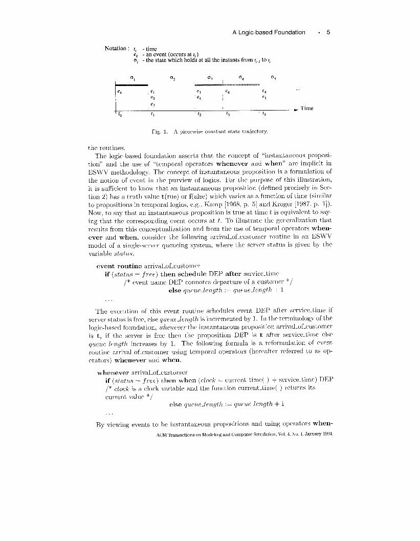
to these aspects can be rcprmented by a picxwvisc constant state trajcct(m~-. As
shown in Fig~mc 1, in a piccewise constant state trajectory, the state changes oIdy
a finit,c number of times, and there arc only fiuitcly mauy uccurrcnccs of tvcnts in
any bounded time interval (hereafter referred to as interval) The kt’Ul T’e[PIWLt
b(lr(ic(or rmlnotcba systrm Ixhavi[m (aIKlmJL arIlc~clelt~ella\ior) rcslrictccltothosc
aspwts of the systmn that arc Ielcwaut to i,hc plmposc of modeling, A dzscretr eoe71t
mrdfl of a system is a set ui mprcssicms in some language. and it slunmarizcs all
rclcvaut system behaviors (hereafter, Ieferrcd to as hchaviors) by accounting for
the changes in state and occur~cnces of m-ents lU an~- state trajectory rcpresmting
a behavior. .411 ESJI”V mocf(’1 consists of’ rmltincs. one for CM-11 type of event,. The
execution of an event routi~le cllangcs valIIcs of some variableh and schedldes or
cancels f~ltlu-c e~rent occllrrcnccs. The order of cxccuti(m of the mutinrs of simul-
taIleollsly(lcclllriIlg events is drtcrminwt based upou the p~imitics associated with
ACkI~msactl[,ns or~NIodc,llng and Cc)mputcr S1ntulat]on, I7ol 4,N0 l, Jimu,aJy 1994
ALogic-based Foundation . 5
Notation : t, . time
~, - m event (occurs at ti)- the state which holds at all the instants from t,., to f,
e4 el el e4 e4.,.
e2 e4 e5e3
* Timet“ t, t2 t3 t4
Fig. 1. A piecewise constant state trajectory.
the routines.
The logic-based foundation asserts that the conecpt of ‘(instantaneous proposi-
tion” and the use of “temporal operators whenever and when” arc implicit, in
ESWV methodology. The concept of instantaneous proposition is a formulation of
the notion of event in the purview of logics. For the purpose of this illustration,
it is sufficient to know that an instantaneous proposition (defined precisely in Sec-
tion 2) has a truth value t(rue) or f(alsc) which varies as a function of time (similar
to propositions in temporal logics, e.g., Kamp [1968, p. 5] and Kroger [1987, p. 1]).
Now, to say that an instantaneous proposition is trl~e at time t is equivalent to say-
ing that the corresponding cveut occlu-s at t.To illustrate the generalization that
results from this conceptualization and from the use of temporal operators when-
ever and when, consider the following arrival-of-customer rol~t ine in an ESWV
model of a single-server queucing system, where the server status is given by the
variable status.
event routine arrival.of-customer
if (status = ,free) then schedule DEP after service_time
/“ cwmt name DEP connotes departure of a customer “/
else qumdength := queue-length + I
The excc~ltion of this event routine schedules event DEP after service-time if
server status is free, else queue-length is incremented by 1. In the terminology of the
logic-based fo~mdation, Aenever the instautamous proposition arrival.of_customer
is t, if the server is free then the proposition D13P is t after service.time else
yueue.l~n.gth increases by 1. The following formula is a reformulation of event
routine arrival-of-customer using temporal operators (hereafter referred to as op-
erators) whenever and when.
whenever arrival-of.customer
if (status = ~ree) then when (clock = current.timc( ) + Service-time) DEP
/* CIOC~ k a CIOCk variable and the f~mction current.time( ) returns its
current value */
else qum~e_len@h := queue-length + 1
.
By viewing events to be instantaneous propositions and using operators when-
ACM ‘Ihnsactions on Modehng and Computer Smmlation, Vol. 4, No. 1, January 1994.

6“ A, Radlya and R, G. Sargent
ever and when. many interesting possibilities arise. In gmerid. a formula F of
the form “whenever c ~“ means that another formula ~ is true or holds at all the
time instants (her-cafter rcf’c[recf to as instants) at which condition c is true. In the
above example, whenever is used to assert that ,f hohis at all the instants at which
arrival-c] f.customer- is true. Similarly when is used inside f to assert that in the
flltru-e when dork has a specified value the proposition DEP is true. The “ESWV
languages” utilize whenever and when in a restricted manner as exemplified in
the above formula. A~l ES IVL’ la~quaye is a simulation language that providm lam
guagc constr”llcts to facilitate the use of ESM’V in describing models. A powerful
generalization emerges if wc allow c to be more complex than a single proposition
such as arrival. of.customer. FOI example in a formula F of the form “whenever cf.,
—If c is (arrival-of-customer & DEP) then formula F states that formula ~ holds
at all the instants at which both arrival. of-cllstomer and DEP occur. Hence. this
fo~ m of formulas can specify iutcraction among simultaneously occurring events.
—The irltmaction among simultaneously occurring ewmts can also be specified in
an alternati~”e manner by a formlda of the following form.
whenever arrival.of.customer
/* specify otht’r effrcts */
if (DEP) then.
In this formula, a rcfcrencc to the truth of DEP occlms inside the formula ~.
-If c is (wE1 & (arrival_of-custonwr or DEP )) then formula F describes what
happ(ms whenever (1) at least one of the events arril-al-of-customer and DEP
occlms and (2) event El does not, occur, (Note that ~ denotes the propositional
mmlect ive “’not,”. )
Similarly a condition associated with the when operator can be any of the abo~rc
conditions.
The above forms of formulas are possibk’ to express and intcrprrt as explained
bccal~se e~’ents are formulated as instantaneol~s propositions. An important gener-
alization in another dimension emerges by lloting that in our natural language we
llse conjunctions whenever au(l when in more sophisticated ways than their im-
plicit usage in DENIS languages. Also, in olu- natural language wc usc many more
conjunction,, filso called operators in logics [Kr-oger 1987: Racliya 1990; \Yolpcr
1983], sllch as next, if, when. whenever. until, while, unless, and at. The
existing practicrs in DEMS can be enhanced by allowing more of these operators.
However. a framew-ork is nee(lcd to answer- questions slwh as — Wlat do opera-
tors mean”? lfrhat is the meaning of expressions containing these operators? How
to simulate models defined l~sing such expressions’? Jtlat is the expressivity of
(liffcr ent operators’?
The logic-based foundation presented in this article does not answer all such
qucstioms but it prwviclcs a framework in which these questions can be meaningfully
raised and answered by defining the basic srmantic concepts of DELIS, a logic LD~
for expressing dis(rete event models, and a simldation procedure for simulating
discrete event moclcls (hereafter called models) that are cxprcssihle in a sllblogic
of L ~)~. It also amwers the following questions which have been s~~ggcsted by-
AC’M TransactIons on Modeling and Ct)rnputer Slmulatlon, \’ol i, No 1, January 19%4

ALogkc-based Foundation “ 7
Barwise [1985, p. 14] as guiding principles for fiuding useful logics. What are the
important semantic concepts’? What sorts of mathematical structures capture these
concepts most naturally’? What sorts of languages best mirror the modelers’ ways
of describing properties of these mathematical struct{wes? What forms of reasoning
using these languages are legitimate? These questions have been answered in this
art icle as follows.
—The important semantic concepts, starting with the two fundamental concepts
of instantaneous propositions (events) and interim variables (similar to piecc-
wisc constant state variables) and culrninat ing into the scrnant ic framework’s
cent ral concept of DE (Discrete Event) structure, are defined. DE st ructurcs
are mat hemat ical structures which capture the important smnant ic not ions im-
plicit in DENIS languages and can be said to be highly specialized and abstract
representations of behaviors.
—A modal Discrete Event Logic LDfj for expressing (discrete event) models is
defined. The logic LDE is defined, independent of its simulation procedl~res,
by specifying its syntax and semantics with respect to DE structures. In LD~,
a model of a system is a set of formulas (expressions of a certain type). The
purpose of the semantics is to specify conditions lmder which a DE strl~cturc can
be said to “satisfy” a model in ~D~. Intuitively, a DE structure (minimally)
satisfies a model if the trl~th values of instantaneous propositions and changes in
the values of interim variables at every instant oft he DE structure are completely
accounted for by the model.
––A simulation procedure for simulating models expressible in a sublogic of LDE is
defined. Simulation is defined to be a process of finding a DE structure that sat-
isfies a given model, and a simulation procedure is an algorithm that defines this
process. The correct ness of a simulation procedure needs to be proven because
LDE is completely defined by its syntax and semantics. In DEMS, a system is
reasoned about using the information obtained from the state trajectories or the
DE structures generated by simulating models. Hence, the current version of the
logic-based foundation provides a tool, namely, a simulation procedure, needed
for the prevalent method of reasoning by performing simulations. Other methods
of reasoning such as verification systems [Ostroff 1989] can be developed in the
future.
A new relaihonshzp among system behaviors. modeling languages models, and
simulation procedures directly emerges from the way in which logics are defined. As
shown in Figure 2, a model is a set of expressions (usually called formulas, rules. or
rout ines ) in a DEMS language. The semantics of a DEMS language specifies con-
ditions under which a mathematical structure abstractly representing the behavior
of a system can be said to satisfy the model. A simulation procedure simulates a
model by finding a mathematical structure that satisfies the model. The correctness
of a simulation procedure needs to be proven with respect to the language defrlli-
tion. These relationships are different from those implied by the existing practice of
defining a simulation language by specifying its syntax and simulation proccclurc.
The logic LD~ cent ains infinitely many operators including next, if, when,
whenever, until, while, unless, and at. Despite the fact that a practicing mod-
eler needs only a few operators, there are both pragmatic and theoretical benefits
ACM Transactions on Modehng and Computer %nulation, Vol. 4, No. 1, January 1994.
8. A. Radiya and R G. Sargent
System behaviors
abstract representation of
[
Mathematical structures
FaiiD_7. Simulationa model by Procedure
I I
I ~1.. . ~ _ mathemat]&lstructure satisfying Lhemodel
LanEuaKe definition
Fig. 2. Relationship among system bebaviors, nlathcmatical structures, exprms,ous of a DELIS
language, aucl simulation procedure.
of defining a logic with infinitely many operators. On the pragmatic side, LDE
provides a better understanding of operators implicit in DELIS langl~ages and al-
lows these operators to be use{l in more general ways. For example, earlier in this
section, our interpretation of ESWV showed more general ways of using whenever
and when operators. Also. if found useful, new operators can be made available
to modelers. For example. unless. although not lltilized in DELIS languages, can
be made available to directly express certain kind of relationships among e~’ent
occrrrrcnces (see Section 5). On the theoretical side, a logic with infinitely many
operators becomw a framework for lmderstanding and analyzing existing waj-s and
for developing new ways of expressing models. The meaning of new operators such
as unless and expressions containing them are already defined by the semantics of
LD~.
In addition to the generalizations rncntioned above, there arc also other advan-
tages of devclopiug a logic-based foumlation of DELIS. First. the large body of
relevant logic-based research work in philosophy and artificial int elligcnce can bc
applied to analyze and cxtertd LDE. Second, it becomes relativel,~ easy to compare
the basic concepts of DELIS with the basic concepts of other Iogics which may,
eventually, Icad to more expressive logics. Third. it may be easier to formally am
alyze LD~ as compared to other simulation languages bccausc logics are formally
defined whereas most simulation langllagcs arc defined by the flow charts of their
simulation procedures. It is difficult to formally analyze and compare simulation
languages when the syntax is partially specified and when semantics is specified by
flow charts. For example. the equivalence of two different simulation procedures of
the same simldation langllage or the claims of expressibility of different languages
usually cannot bc proven when languages am not defirwd formally.
The rest of the article is organized around the questions cnlistcrl earlier in this
section for finding useful logics. Section 2 answers What are the wnportant serno,ntw
concepts by defining the flmdarnental concepts of DEMS and a simple and intuitive
representations of behaviors, called discrete event trajectory. Section 3 defines more
ACM ‘Ikmsactmns on Modeling and Computer Slmulahon, Vol 4, No 1, January 1994

ALogic-based Foundation “ 9
semantic concepts and DE structures which are highly abstract representations of
behaviors to answer What sorts of mathematkal structures capture these concepts
most naturally. Section 4 defines LDE’s syntax and semantics with respect to DE
structures to answer What sorts of languages best mirror the modelers’ ways of de-
scribing properties of these mathematical structures. Section 5 contains nontrivial
example models intended to show modeling capabilities and limitations of LDE. An
answer to What forms of reasoning about LDE are legitimate is given by defining
a simulation procedure for a sublogic of LDE in Section 6. The relevant research
work is discussed in Section 7. Finally, Section 8 summarizes the article and dis-
cusses some research direct ions. Appendix A cent ains two tables which define the
interpretation of symbols used in this article for standard and nonstandard con-
cepts, respectively. Only the not ation for nonstandard concepts is formally defined
in the sections where they are first introduced. Appendix B defines quantificational
functions denoted by commonly used operators. Appendix C contains a model
of a preemptive single-server system in L~E which does not utilize the temporal
operator unless.
2. FUNDAMENTAL CONCEPTS AND DISCRETE EVENT TRAJECTORY
The first step in developing a logic-based foundation is to identify the important se-
mantic concepts and define them in the purview of logics. The two logical concepts
of instantaneous proposition and interim variable are considered to be the most fun-
dament al. These concepts are the basis for defining (system) behaviors, developing
other semantic concepts implicit in simulation languages, and constructing models.
Section 2.1 formally defines these concepts and Section 2.2 defines representations
of behaviors called discrete event trajectories.
The following definitions and notations are used in this article. First, four types
of intervals arc defined. Let i, k ● R+ and j E (R+ U {cm}) or i, k E N and ,1 ~
(N U {co}), where R+ is the set of nonnegative real numbers and N is the set of
nonnegative integers. The four types are:
[i, j]={kli<k<j,.j#m}, (i, j]={kli<k S.j, j#m},[i. j)={kli<k<j}, ancl (i, j)={kli<k<j}.
The syntax of a universally quantified sentence is (’dvl, V2, . . . . vn : c1 ) [CZ] and it
means that any tuple of values of variables V1, V2, . . . , Vn which satisfies condition c1
also satisfies condition C2. Hence, it is equivalent to (’dZJl, 2)2, . . . . Vn ) [cl + C2]. The
notation of “exp = (if c then expl else ezp2)” means that the value of expression
ezp is the same as the value of expression ezpl if condition c is true; ot hcrwise, it
is the same as the value of expression exp2. In writing tuples, symbol “.” means
that any acceptable value can be substituted in its place. For example, a tuple (:x,
-) of type Vail x Va12 means that the second element can be any value from set
Va12.
2.1 Fundamental Concepts
The concepts of instantaneous proposition and interim variable are a formulation of
t hc widely known concepts of event and piecewise constant state variable, respec-
tively. The formulation of events as instantaneous propositions which have truth
values allows logical combinations of events. The formulation of piecewise constant
ACM TransactIons on Modeling and Computer Simulation, Vol. 4, No. 1, January 1994.
10 . A. Radlya and R, G, Sargent
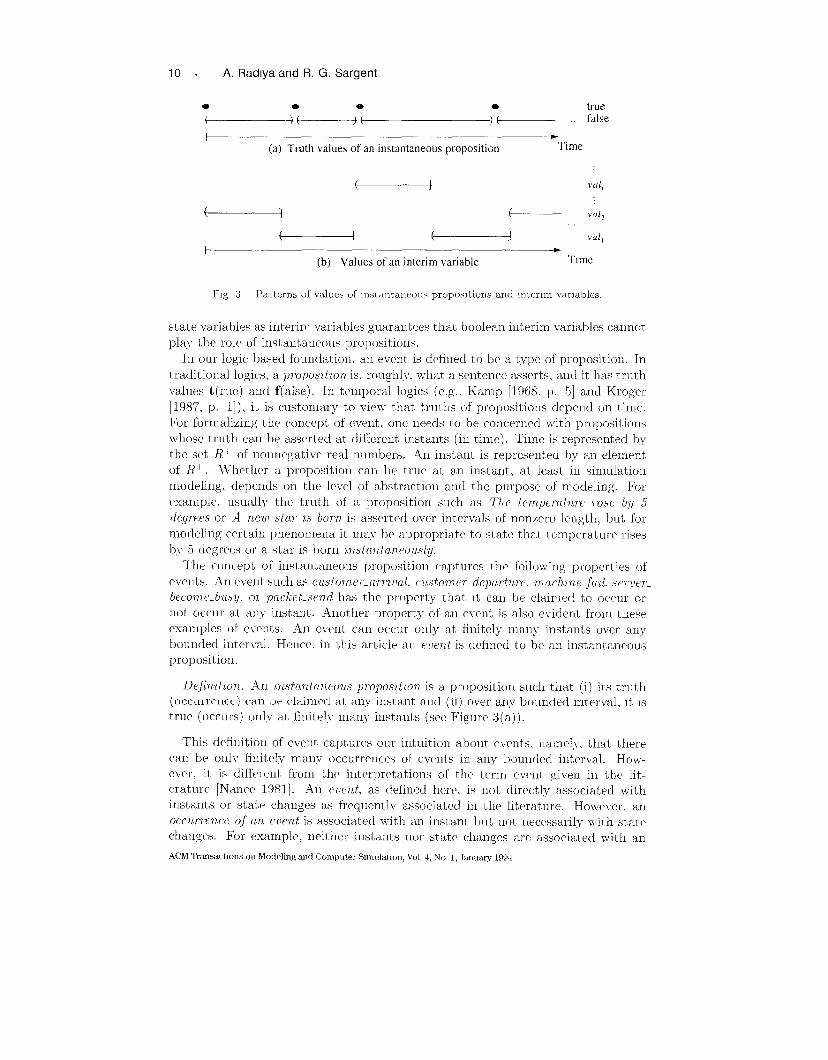
I -—
(a) Troth valws of an instantaneous proposition Time
(~ Vul,
( 1 ~’ vul*
(~ (~ V(I1,
{ +
(b) Values of an interim variable Time
F,g 3 Pattern~ of values uf instantancn(m propositions and mterlm \,arIablcs
state variables as interim variables guarantees that boolean interim variables cannot
play the role of instantamwlw propositions.
In our logic-based foundation, an event is drfinecf to be a type of proposition. In
traditional logics, a propos2tzon is, rollghly, what a sentence asserts+ and it has trllth
values t (rue) ad f(alse). In temporal Iogics (e. g., Kamp [1968, p. 5] and Kroger
[1987, p. I]), it is customary to view that tr~~ths of propositions depend on time.
For formalizing the concept of event, one needs to be concerned with propositions
whose truth can be asserted at different instants (in time). Time is represented by
the set R+ of nonnegative real munbers. An instant is represented by an element
of R+. ~Vhethcr a proposition can be true at an instant, at least in simulation
modeling, depends on the level of abstraction and the purpose of modeling. For
example, usually the truth of a proposition such as The temperat?tire rose b;l~ 5
degrees or A neu) stur M born is asserted over intervals of nonzero length, but for
motlcling cm-tain phenomena it may be appropriate to state that temperature rises
b~- 5 degrees or a star is born ?n.st(rrlfant’c]usly,
The concept of instantaneous proposition captures the following properties of
events. An evel~t such as cusf[jmer-o,rrt[l(~,l, custom er-departure, mochzne-fd sm-ven
bwomt>-b[ls?y, 01 packet-send has the property that lt can be claimed to occur or
not occlu at an~- instant. Another property of an event is also evident from these
examples of events. An event can occur only at finitely many instants over any
bounded interval. Hence, in this article an erwnt is defined to be an instantaneous
proposition.
Definzflon, AI1 Instantaneous prqmsrt/on is a proposition such that (i) its truth
(occuri-enc c) can be clairnrd at any instant and (ii) over any bolmcfed interval, it is
trllc (occurs) only at finitely many instants (see Figure 3(a)).
This definition of event captures our intuition abollt events. namely, that there
can be only finitely many occurrences of ev(,nts in any boun[lecl interval. How-
cvrr, it is differ cnt from the int crpretations of the term event given in the lit-
erature [Nancc 1981]. .411 e ~]ent, as (lefincd here. is not directly associated with
i~lstants or state changes as frequently associated in the literature. How~ver, an
occurrence o,f an eilen,t is associated w,ith an instant bl~t not Ilecessarilv with stat,e
changes. For example, neither instants nor state changes are associated with an
ACM ‘L’mnsactmns cm Modeling and Computer Slmulatlon, Vul 4, No 1, January 1994
ALogic-based Foundation “ 11
event custom, er-arriljal per se but its occurrence must be associated with an in-
stant. Also, certain occurrences of customer-arrivals ucb as those coinciding with
customer.departure may not be associated with state changes, e.g., the number of
customers in the system may not change. Note that events as defined above do not
include the paramet erizcd events such as the rnachine_break.s_down (i). Ncmet heless,
a parameterized event can be represented by a set of instantaneous propositions or
nonparameterized events. For example, machine_ breizks.down (i) is equivalent t o the
set {machine-l-breaks-down, machme_2_breo,ks_d own, machine_3_breu,ks_d own,. ..}.
The concept of an interim variable is a particular formalization of piecewisc
constant stat e variables. The concept of a piecewise constant stat c variable is
defined in the literature to be a variable which holds the same value for an interval
of time [Zeigler 1976]. Recall that there are four types of intervals based on whether
an interval is closed or open on the left and right ends oft he interval. The following
definition of an interim variable places restrictions on the ends of intervals over
which it has the same value. This restriction is sl~ch that a boolean interim variable
does not eschew the concept of instantaneous proposition.
Dejinitton. An interim varzable v is a variable such that (i) it is meaningful to
claim that v has a value at any instant and (ii) over any bounded interval 1 that is
open on the left and closed on the right, z!’s value changes only finitely many t imcs,
and every maximal subinterval of 1 over which z] has the same value is open on the
left and closed on the right (see Figure 3(b)).
Some examples of interim variables are q-length, q-length-ts-~, and server-u-busy.
Note that q-length-@ and server-wbusy are boolean interim variables because
their values can be either t or f, whereas q-length is not a boolean variable because
its value can be any element in N. A boolean interim variable t] cannot play the
role of an instantaneous proposition because if ~) has the value t (true) only instan-
t aneously, say at an instant t,then it is f (false) in a maximal interval ending at t
which is open on the right. Hence v is not an interim variable. In the remainder
of the article, variables are interim variables, and propositions are instantaneous
propositions.
2.2 Discrete Event (DE) Trajectory
A behavtor of a systcm is defined by the values of (instantaneous) propositions and
(interim) variables at all the instants of an interval. The nurrlbcr and meaning
of propositions and variables depend on the purpose of modeling. Discrete event
modeling and simulation utilizes computers. and hence, it is necessary to assume
that a set of propositions P and a set of variables Vur representing the aspects of a
system that a modeler is interested in are finite. This finiteness assumption and the
definitions of proposition and variable imply that, in any bounded interval. there
are only finitely many instants at which either a proposition is true or the value
of a variable changes. A representation, called dzscrete event trajectory, completely
describes a behavior by specifying the values of propositions and variables at these
instants. The values of propositions and variables at an instant are defined by
valuations.
Definition. An instantaneous valuatton is a function of type P - {t,f}, where P
is a finite set of iust ant aneous propositions. An instantaneous valuation is denoted
ACM TransactIons on Modehng and Computer Wnulation, Vol. .4,No. 1, .January 1994
12 - A. Radiya and R. G. Sargent
by t, possibly with a numerical subscript, and the set of all instantaneolls valuations
by 2.
Definztzon. An ~nter~m tuluatton is a function of type I’ar ~ ~’al, where Var is
a finite set of variables, and l-al is a set of values. An interim ~aluation is denoted
by 6, possibly with a numerical sl~bscript, and the set of all intcmm valllations byed.
An instantaneous valuation is represented by a set of propositions that are true
in it, and an interim valuation is represented by a set of elements of the form ?Iur =
L]al, For exalIIPle, consider a single.server queucing system as defined by the set of
propositions P = {.-l, D} which correspond to the events of arrival and departure
of a customer, respectively, and a set of interim variables l-ar = {status, ql} whose
values denote the status of the server and the length of the quww, respectively.
For this system, the set ~ consists of valuations ~, {A}, { D}, and {A. D}. Some
example interim valuations are {.$tat~~s = fr~e, ql = 0} and {status = htlsy,
ql = 9}. Now, a discrete event trajectory is defined in terms of valllations.
Definition. Let I C R+ be an interval which is closed on the left and to E I t)e
its smallest clement. A D~tscrete llueut (DE) tmjectory over an interval 1 is a list
of tuples ((tiu, 6.. to), (61, til, tl),. .), where 61 E E, 6L = E, and t~ = 1. such that,
to < tl < tz and only finitely many t,’s are contained in any bounded subinterval
of 1.
The transztioa instants of a DE trajectory H arc defined to be positions in list
H and are denoted by set {0, 1. 2,. ... IHI – 2} = [0, IHI – 1). A stateat a
transition instant i is defined to be the t uple (d,, @t, t,). Figure 4 shows the DE
trajectory representing a behavior of the single-server system defined above. In
the diagrammatic representation of a DE trajectory, an instantaneous valuation is
represented by a triangle, and an interim valuation @T is represented by an arrow
of the shape + going from t7–1 to t~. For an instantaneous valuation, only true
propositions are shown. Hence, triangles appear only at the transition irlstants
because at any other instant, all pI opositious are false. However, it is possible that
all propositions are false at a transition instant. An interim valuation 6, is placed
at the end of+. The symbol “(” signifies that 61 holds at all the instants from just
after t ,– 1 (exclllded) to t, (included). The transition instants of a DE trajectory
are shown at the top and the associated clock times are shown at the bottom.
A value of a proposition or a variable at any instant in a DE trajectory can be
easily obtained. For any proposition p and clock time t,if t = t,,then the truth
value of I is b, (p): otherwise it is f. For any variable t, and clock time t > tu, the
value of t) is iTn ( ~~), where n is the largest possible vallw such that t,,–1 < t;for
clock time to,the value of z is Do(~)). For example, in Figlu-e 4, the truth value
of proposition .4 RRIWIL at instant tl is t and at any t: (tl < t < t2) is f. The
value of ~ariable ql is 1 at any t: (t~ < t < tz) because ql is 1 in tin with n = 2 and
because n is the largest value such that tn–~ = tl< t.
3. DISCRETE EVENT (DE) STRUCTURE
In this section, a highly specialized and abstract representations of behaviors, called
Discrete Event (DE) structures, are defined by extending the representations of DE
ACM Tmmsactmns on Modeling and Computer Simulation, Vol. 4, No 1, January 1994
A Logic-based Foundation . 13
Notation: Interim variables -S:slatus, ql:que~e_length
Instantaneous propositions - A : arrival _of_customer, D : departure_of_customer
5.= 64={ S= free, ql= O), 62 = {s= busy, ql= 1),
6, = 63 ={S = busy, ql= O), 6, = 61+1”= i71+z={S= busy, ql= 9].
o 1 2 3 i i+l
Fig. 4. A DE trajectory of a single-server queueing system,
trajectories using transitions. The DE structures are the mathematical structures
with respect to which the semantics of LDE is defined in the next section. In the
literature, a transition is commonly defined to be a function from states to states
[Zeigler 1976], or equivalently, from interim vall~ations to interim valuations. In
this art icle, two types of transitions, called primitive-transitions (p-transitions) and
extended-t ransit ions (e-transitions), are defined. The intuition for defining these
transitions is given below by considering the use of expressions like {whenever c
~} in modeling. Recall that {whenever c ~} is a logical formulation of an event
routine in an ESWV model and it means that formula j holds at each instant at
which condition c is true. For giving the intuition abol~t transitions we consider
what is commonly expressed by j about interim variables at a transition instant L
in a DE trajectory H at which the condition c is true. Let (ti,, tit, t,) be the state
at i.
(1)
(2)
(3)
(4)
Formula f defines values of some variables in 6, + ~ as a function of F,. For
example, the event routine arrival-of-customer in Section 1, may define t hc
value of variable queue-length in ~,+1 as a function of the values of variables
in 5;.
Formula ~ utilizes some basic mechanism such as a single-assignment statement
to define values of some variables in 6,+1 as a function of ~,.
Formula f also utilizes some advanced mechanisms such as conditional and itcr-
at ive statements. The effect oft hese mechanisms is that values of some variables
in ti,+l are defined by jintte applications of basic mechanisms in sequence. For
example, a while-program {while (x < 5) {z := z + 1}} increments the initial
value of ~ from. say O to 5 by applying the basic mechanism of incrementing z
by 1 for a finite number of times in sequence.
A model, in general, consists of several event routines, or, equivalently, several
formulas of the form {whenever c f}. Hence, two or more formulas may be
applicable at a transition instant i if their conditions are true at z. This is
acceptable as long as the formulas are not inconsistent, i.e., the formulas do
not define different values of the same variable. Hence, it must be possible
ACM Transactions on Modeling and Computer Siiulatlon, Vol. 4 No 1,JanuaIY 1994.

14 “ A. Radlya and R, G Sargent
to compose what is accomplished in the above statements 2 and 3 in pwml-
lel. For example, the formldas (1) {whenever (13VENT1) {r := .~ + 1}},
(2) {whenever (EVENT2) {y := ?)+ 1}}, and (3) {whenever (EVENT1 &
EVENT2) { {.~ := % + 1}; {y := {J + 1}}} itr~ applicable at a transition instant
z if EVENT1 and EVENT2 occur at {. These formldas are not inconsistent
because if :r = 5 and y = S in F, t lwn both the fo~ mldas (1) aml (3) define the
vallw of ~ to be 6 in @,+1 and both the formulas (2) and ( 3 ) defhlc the vallw of
y to be 9 in 0,+1.
The first two of the above four statements arc the basis for defining p-transitions
as functions from interim valuations to simple-substitutions (s-substitll’cions ). where
an s-substitlltion defines values of some variables. lVC luw the term s-sllhstitution
to indicate the fact that an s-substitl~tiou is a simpler form of a general substit,lltion
[Robinson 1979]. An s-substitl~tiou is simpler because it associates only constant
l’alllcs with variables. The last two of the above folu statements are the basis
for defining the concept of c-transition as a physical arrangement of p-transitions
using the common mathematical concepts of set and sequence which as shown below
correspond to parallel and sequential composition of lJ-transitions, respectively-.
De,fin~tton,. A .szmple-is!lbst~t?Lt~on (.?-s?Lbst!t~l,tLo’rt) is a partial function ot typ(:
~“ar 4P Iral. An s-substitution is denoted by 0. possibly with a numerical sub-
script, and the set of all s-sl~bstitllt,ions by ~.
An s-sllbstitl~t ion is represented by a finite set of the form {11/ La[l, . . . . ~,, //al,,},
where ~’, ● Var and I!al; E ~~ul is the value of t,. If ~!,/zal Z is in (the represent atiou
of) 0 then u, is said to be bound in (). .4n s-substitution (iefines val~ws of some
variables and it can be interpreted to specify the difference between two interim
valuations or the changes that, must be made iu a given intm-im valuation to obtain
another interim ~’all~ation. The latter interpretation is formally defined by the
COIICCpt of a variant of an interim valuation,
For example, in the single-server system (Iefine(l in Section 2.2, I“ar = {stat US,
qi}. Two example s-substitutions are t?l = {stat us/~ree} and 9! = {stat us/bus,y,
ql/20}. If interim valuation F = {.$tatus = btfs,y, ql = O} then 6’s variants are
ti(f?l) = {status = free. ql = 0} and 7(02) = {status = busy, ql = 20}. In fi(O1).
status is free because status is bound in @l and HI (stat li.s) = free , whereas ql is
O because ql is not bound in #l and D(ql) = O.
Definition. A primitive transztwn, (p-trwnsiiwn) is a total function of type ~ -
0. A p-transition is denoted by 6J, possibly with a numerical subscript, and the set
of all p-transitions by Tp.
For example, p-transition pl corresponding to assignment statement {status :=
busy} is pl (6 ) = {stafus/busy} and ,fJj corresponding to statement {if (status =
b~{.~y) then ql := ql + 1} is pz(~) = (if ti(status) = btlsy then {ql/ti(ql) + 1} else
GO)
ACM ‘kmsactlans on Modehng and Computer Simulation, Vol 4, No 1, January 1994
ALogic-based Foundation - 15
Defi’nit%on. Thesetof all extended-transitions (e-transitions) TEis defined recur-
sively.
TE={(), ({ f~}), (El, E2,..., En)lfo GTpandn ~Niss~~chthatn>0
and fori=l ,2,... ,n, E, <T~ and IE, I > O}
An e-transition is denoted by e, possibly with a numerical subscript, and a set of e-
transit ions (~ TE ) by E, possibly with a numerical subscript. For any e-transition
e, Ie I denotes the number of elements of e. The e-transition ( ) is called the empty
c-transition and ({p}), where p E Tp, is called a szmple e-transition.
An e-transition is a finite, possibly empty, list of finite nonerupty subsets of TE.
The simplest e-transition corresponding to a p-transition ~J E TP is ({p}). An
c-transition is au arrangement of finitely many p-transitions using the concepts of
set and list or sequence. The concept of set embodies the parallel application of
transitions, whereas that of list embodies the sequential application. However, an
arrangement can be arbitrarily nested. For example, if f~l and gJ2 are p-transitions
then el = ({({ ~Jl }) }, {({ p~ }) }) corresponds to the application of fol and (J2 in
sequence and ez = ({({ pl }), ({ pz }) }) corresponds to the application of pl and p~ in
parallel. Note that Iel I = 2 and Iez I = 1. The e-transition ({e], ez }) applies el and
ez in parallel which means that the entire application of PI and pz in sequence due
to Cl occurs in parallel with the entire application of (Jl and @z in parallel due to ez.
An e-transition can also bc viewed as a finite way of specifying how some variables
of an interim valuation are to be changed by applying p-transitions in parallel and
in sequence. An important difference between the two types of transitions is that
p-transitions are total functions of type Z ~ @ whereas e-transitions are partial
functions of type X 4P 6. The modification function AI as defined below returns
the partial function of type X +P @ that is associated with a given e-transition
For defining function M and applying trausit ions in parallel and in sequence, it is
neccssar-y to define nonconflict iug substitutions and composition of substitutions.
Defimtton. Two s-substitutions 61 and ~z are nonconflicting iff for all v bound in
both 9] and i32, 91 (7)) = 02(v). A set of s-substitutions S ~ @ is nonconflicting iff
every pair of substitutions in S is nonconflicting. A variant of an interim ualuation
5 under a set of nonconflicting substitutions S is 6(S) = 6(U {6’ I 19E S}).
Definition. The composition of two s-substitutions 01 and ~z denoted by 191 “ Qz
is the s-substitution {v/c I v is bound in either 61 or 192, and if 1] is bound in 192
then z/c c 62 else L1/c c O1}.
For example, substitutions t)l = {ql/1 } and 02 = {status/free} are nonconflict-
ing; hence, 81 U & = {ql/1, status/free} = OL “ 82,. However, f3s = {ql/2} and 61
are conflicting; hence 61 U 03 is not defined, but 61 “ 03 = {ql/~} and 63 0 61 =
{ql/1} are well defined.
Defirution. A modijicatton junction AI : TE 4 (E +P e) is defined by induction
on the structl~rc of the elements of T~. If e E TE is such that Iel # O then let e =
AOM Transactions on Modeling and Computer %nulation, Vol. 4, No. 1, January 1994.

16 . A. Radiya and R. G. Sargent
Notation : Same as in Figure 4.
p-transitions : @, (G) = {S&ree), @z(@ = {qVN-1}, where ql=Nin 6,
P,(5) = {Ybusy), @4(@ = {qVN+l], whereql= Nin 6
e-traflsi[ioflS : t!, = ({ ({ fol} )} ), ez = ({({ K321)}),
~3 = ({({ tJ3} )}), e4= ({({04}}})
o 1 2 3 i i+l
— — —Go 01 ~1 ~3 ~4 6, G,+, 5,+2
/ w . . .( w * . . .
\
ElE,={)= E,+,
* Time
Fig. 5 A Discrete E\,ent (DE) structure K over interval 1.
({cl,...,e,,}) oe’, wherenz 1 and el,..., en, e’ c T~.
I@ if’ Iel = O
~J(ti) if e ~ ({ fC)}) and gJ ~ Tp
M(e)(5) = (U1<7<,, {AI(e, )(~)}) AI(e’)(fil ) if Iel #O and the condition (c)
given below is true
undefined otherwise
(c) = (1) the set of s-substitutions {A1(el )(6) I 1 5 2 S n} is defined and is
noncoufiicting and (2) M(e’ ) (til ) is defined, where al = 6(U]s, <r, {A~(ej )(@)}).
Dt!finatlon. An c-transition F is well-defined for an interim wdlmtion F iff Lf(e) (~)
is defined.
For example, if pl (ti) = {ql/D(ql) + 1} and pz(~) = {ql/3} then an e-transition
e = ({({jJ~})}, {({g~l}). ({p2})}) is well-defined for @o = {qi = 1} t)llt not for til
= {ql = 2} because for @~ = ti~ (lU(({fJ~}))(6~)) = m~(p~(~l)) = {ql = 3}, pl(i72)
= {gl/-l} and f]~(ti~) = {ql/3} arc conflicting.
Now, DE structures are defined by connecting every pair of adjacent interim
valuations of a DE trajectory H by a nonempty set of c-transitions.
[email protected]. Let I G R+ be an interval which is C1OSCCI on the left, to be the
smallest element of 1, and EI = ((cio, ~o, to)) (til, @l, tl), . . .), where b, E ~. 6, E ~.
and t,E I, be a DE trajectory over I. A Dtscrete Event (DE) strwcture K over
an interval 1 is a tuplc (H, X), where X is a list (E., El, . . .) of nonempty sets of
e-transitions (E, C T~) such that
IX = IHI -1 and ~,+~ = C7,(UISJS,, {AI(el )(u)}), where i >0 and
E, = {eI,. ... en}, n> 1.
The transition instants and state (ti,, 6,. t,) at a transition instant i of the DE
structln-e K arc defined to be the same as in its DE trajectm--- H. The cardinality
ACM ‘llansactmns cm Modeling and Computer Simulation, Vol 4, No 1, January 1994
ALogic-based Foundation o 17
of K is defined as IK I = IX I and it represents the total number of transition instants
in K. A pictorial representation of a DE structure is a pictorial representation of
a DE trajectory with boxes representing e-transitions at the transition inst ants.
In general, many DE structures can be associated with a DE trajectory. One of
the many possible DE structures corresponding to the DE trajectory in Figure 4 is
shown in Figure 5.
The DE structures are the mathematical structures used for defining the se-
mantics of logic LDE in the next section. The above definition of DE structure
requires the concepts of instantaneous valuation, interim valuation, s-substit ut ion,
p-transition, and e-transition. These concepts have been defined hierarchically
starting from the concepts of instantaneous proposition and interim variable. The
intuition for the need of these concepts was given at the beginning of this section.
4. MODAL DISCRETE EVENT LOGIC LDE
The logic-based foundation’s modeling language modal D~screte Event Logic LDE
is defined in this section. As explained below, LDE generalizes some of the ways
in which models in DEMS languages summarize (relevant system) behaviors. A
model summarizes behaviors by accounting for event occurrences and changes in
values of variables at every transition instant of any DE trajectory representing a
behavior. Different DEi’vE3 languages provide different constructs for summarizing
behaviors. The logic-based foundation views that the purpose of these constructs,
called modeling co?~structs, is to (1) refer to transition instants in a DE trajectory
and (2) assert occurrences of events and/or changes in the values of some variables
at t hcsc instants.
In DEMS languages, the transition instants are referred to by implicitly utilizing
only a few (temporal) operators in a limited way, and the changes in the values of
variables at a transition instant are defined by composing finitely many p-transitions
in s~quence. Recall from Section 3 that a p-transition is a function which defines
(changes) values of some variables, given the values of all variables. The logic LDE
generalizes the ways of expressing models in DEMS languages by using operators
implicit in DEMS languages in a more comprehensive manner, new operators, and
logical conditions on instantaneous propositions, interim variables, and time. It also
allows changes in the values of variables to be defined by composing finitely many
p-transitions in parallel and sequence (see the concept of e-transition in Section 3).
In the following, the syntax of LDE is defined in Section 4.1. Then, the semantics
of LDE is defined with respect to DE structures in Section 4.2. The syntax and
semantics of LDE are illustrated in Sections 4.1 and 4.2, respectively, using a model
of a single-server queueing system. Two models of a nontrivial system intended to
show new ways of summarizing behaviors are discussed in Section 5. (The mat hc-
matical details in Section 4.2 can be omitted if only an intuitive understanding of
the subject matter is desired.)
4.1 Syntax of LDE
The logic LDE’s syntax consists of an alphabet which defines various types of
symbols and a set of rules which define various categories of expressions including
the category of formulas. In LDE, a model is a set of formulas. Before specifying
the complete syntax of LDE, we intuitively describe the ways in which formulas
ACM llansactlons on Modeling and Computer Smulation, Vol 4, No. 1, January 199-I

18 . A. Radlya and R, G Sargent
and other types of expressions embedded in formulas refer to transition instants
and assert occurrences of events and/or changes in values of variables. Recall that
behaviors are denoted by DE trajectories/structures. A formula can be of the form
{a~}j {0 c j,}, {~~ II ~~}, {~~ ; .f~}, or {p}. where a,f is an action-formula; o is an
operator; c is a condition; p is an instantaneous proposition symbol; and ~1 and
~z are other formulas. Action-formulas are defined in the same way as formulas
except that they utilize only interim variables and do not utilize the variable clock
and instantaneous proposition symbols. A formula is enclosed in {. ..} and an
actio]l-formlda is enclosed in [. ..1.
(1) Referrmq to transztmn Instants:
(a) A logical condition c on propositions, variables, and time refers to a set
S of instants at which c is true in a DE trajectory. For example, if c is
(EVENT1 & (ql = 10) & clock < ham) theu every instant before llarn
at which EVENT1 ocmu-s and ql has value 10 is contained in S.
(b) An operator-phrase “o c“ refers to a set S’ of instants that arc related to
S by a temporal op~’rater o. For example, for “whenever c“, S’ = S’, i.e.,
S’ contains all the instants at which c is true. For “when r“. S’={ilzis
the least clement of S}. i.e.. S’ contains only the earliest instant at which
c is true.
(2) Asserting omurr~rLce.s of events andior changp,s /n takws o,f lmrzables uszrtg
f r-unsitlons:
(a) A formula of the form {o c ,f} asserts that formlda j holds at each instant z
in the set S’ denoted by o c. Now. ~ being true at 7 may assert occurrences
of events and transitions at 1 and in the future of t. If formlda ,f has the
form {p} then inst antancous proposition p is asserted to be true at i, If ,f
has the form {a,f }, where af is an action-formula, then a possibly complex
transition is asserted at i.
The truth of ~ at r can assert event occlmrcnces and transitions in the
futl~rc of i because ~ can bc any formula in LD~ including a formula of
the form {ol c1 j’l}. For example, let {o e ~} bc {whenever (EVENT]
& (ql = 10) & clock < ham) {when (clock = cllrrent_tinlc( ) + tl)
{EW3NT2}}}. Then. {o c ~} asserts that forrmda ,f. i.e.. {when.. .},
holds at all the transition instants at which condition c is true. If c is
true at instant t then EVENT2 occlu-s at the ftlturc instant t + t] becalusc
,f holds at t. Similarly, if formula {when (clock = curren_time( ) + t,)
{ [[-r ‘= ~ + III}} i=tr~~~at ill+ant t in a DEStructurethenit asserts thata transition which increments .r by 1 occurs at the future instant t+ tl in
the DE structure.
(b) A formula of the form {~1 II ~z } allows a modeler to combine event occur-
rences and transitions asserted by ~1 and ~z in parallel, whereas a formlda
of the form {jI ; j?} combines cveut occlu-rences an(l transitions asscrtecl
by ~1 and jz in sequence. For example, let ~1 be {when ( c/ock = rur-
rcnt -timc( ) + t1) {EVENT1 } }, ,fil be {when (clock = current -tirne( ) +
t2){{[[r := T + 1]1} II{EVENT2}}}, and curren.time( ) be t. Then.
{./’1 II .f~ } asserts that at t + fl, EVENT1 occurs and at t + tz, EVENT2
ACM Tmnsxtmns on llfodchng and Computer Slmulatlon, Vol 4, No. 1, .Janua.ry 1994
ALoglc-based Foundation o 19
occlu-s andthevall~eof.c increases by 1. However, {,fl ; ~z} asserts that at
t+tl, EVENT1 occurs and at t+tl +tz, EVENT2 occurs andthevaluc
ofz increases by 1. (It must be noted that in LDE, parallel applications of
two formula s.fl and~l areinclcpcndent andclonot follow theiuterleaving
model of parallel computation [Hoare 1985]. ) To further illustrate the con-
nective 11,consider theapplication of LDE fornlulasfl = {[[~ :=x+ l]l}
and jz = {if (O < z < 2) {[[.z := z x 2]1}} at transition instant i with 6L =
{z =0,9=2}. Thcapplication of~ldefi~les ztobclin @,+l, wllereasthc
application of ~z does not define a value of ~ or y because the condition
(O < x < 2) is false in 7,. However. the application of ,fl at transition
instant i + 1 defines x to be 2 in @,+z and the application of ,fz at i + 1 also
defines ~ to bc 2 because the condition (0 < x ~ 2) is true in til+l. Hence,
the applications of ~1 and ~z are consistent for 7, and a,+l. In constrast,
the applications of ~1 and ~2 are inconsistent for @,+z because ~1 defines z
to be 3 in 6,+3, whereas the application of ,fz defines x to bc 4 in 6,+3.
In the above examples, values of variables are changed in a simple way, namely,
using an assignment statement. However, action-formulas of LDE can change val-
ues of variables by applying transitions in sequence and parallel. In the syntax
LDE, transition-terms are defined by enclosing action-formulas in square brackets.
This has the same purpose as enclosing programs in begin. . end in the procedural
programming languages.
AlphabetAn alphabet consists of the following classes of symbols:
P Set of instantaneous proposition symbols.
Const Set of constants.
Var Set of variable names.
Func Set of in-ary function symbols, for each m >0.
Rel Set of m-ary relation symbols, for each m >0.
TO Set of temporal operator symbols. These include next, now, null,
if, when, at, until, while, whenever, unless, and some.
Special variable clock and function symbol current_time( ).
Propositional conucctives N, &
Parallel connective IISequential connective ;
Punctuation symbols [1[1,{,}Categories of expressions
The categories of expressions are operator o, term te, condition c, timed-coudition
tc, interim-condition irw, operator-phrase op, interirn-operator-phrase top, transition-
term tt,action-formula af, and formula ~. The following symbols (possibly sub-
scripted) are used for defining the syntactic rules: to 6 TO, const G Const,
v & Var. g E Func is an m-ary (m > O) function symbol, r E Rel is an ‘m-
ary (m > O) relation symbol, and p E P is an instantaneous proposition symbol.
ACM Transactions on Modeling and Computer Slmulatlon, Vol 4, No. 1, January 1994.

20 “ A. Radiya and R. G. Sargent
RO. O+t(j
RI. te + const I II I ,g(tel,. . . . tern)
R2. c+pl’r(tel,. ... tem)l~c~lc~ &cQltc
tc + Consists of conditions involving the variable clock and real corl-
stant, function, and predicate symbols including clm-cnt .t ime( ).
inc - r(tel,. . . . tern) I N ~ncl I 77XI & inc~
R3. rlp+clc
iop + o anc
R4. tt - [t:= te] I [af]
R5. af A [ttl I [Lop afll I [u,fl II af21 I [~~.fl ; fl.f21I [,flR6. f + {a.)-} I {w fl} I {,fl II,f2} I {.fl ; .f2} I {P}R7. A model is a set of formulas.
The above syntax gives only the schema fur the expressions of the category of
timed-conditions. The main reason for this is that the prmise syntax of timc(l-
conditions depends on both the functions and predicates on real numbers that are
allowed by an implementation of LDE. In the remainder of the article. (boldfaced)
Rn.m refers to tile mth choice in syntactic rule Rn. For example, R6. 3 refers to
{fl IIf2}For the purpose of illustrating the semantics of LDE in the next section, a model
of the single-server queueing system defined in Section 2.2 is described in the syntax
of LDE. A formula of the form {after r-eol.expr p} is an abbreviation of {when
clock = cllrrent -timc( ) + rerr-expr {p}}. where I) is an instantaneous proposition
symbol. ~omments are enclosed in /*. .*/.
Instantaneous propostt%on symbok:
ARR — ARRival of a customer
DEP —- DEParturc of a customer
Infemm Vmvubles:
status: {busy, free} — status of the server
q]: N — length of the qllelle excluding the customer being served
Functzons:
interarrival( ): R+ — A function for the interarrival times of customers
servicc( ): R+ — A function for the service times of customer-s
/’ Initialization formula “/
O. { [~[[status := free]l ; [[q/ :=0]11 ; [{after intcrarrival( ) ARR,}ll }
1. {whenever ARR {after interarrival( ) ARR}}
/* Only arrival occurs “/
2. {whenever ARR & wDEP
2.1. { [ [if status = j’ree [[[status := busy]l ; ~{after service( ) DEP}l 11 II
2.2. [if status = b?isy ([ql := ql + 1]1]1 }} /* formulas 2.1 and 2.2
are connected by II */
/“ Only departure occurs “/
ACM ‘lkmsactlons on Modeling and Computer Simulation, Vol 4, No 1, January 1994
ALoglc-based Foundation “ 21
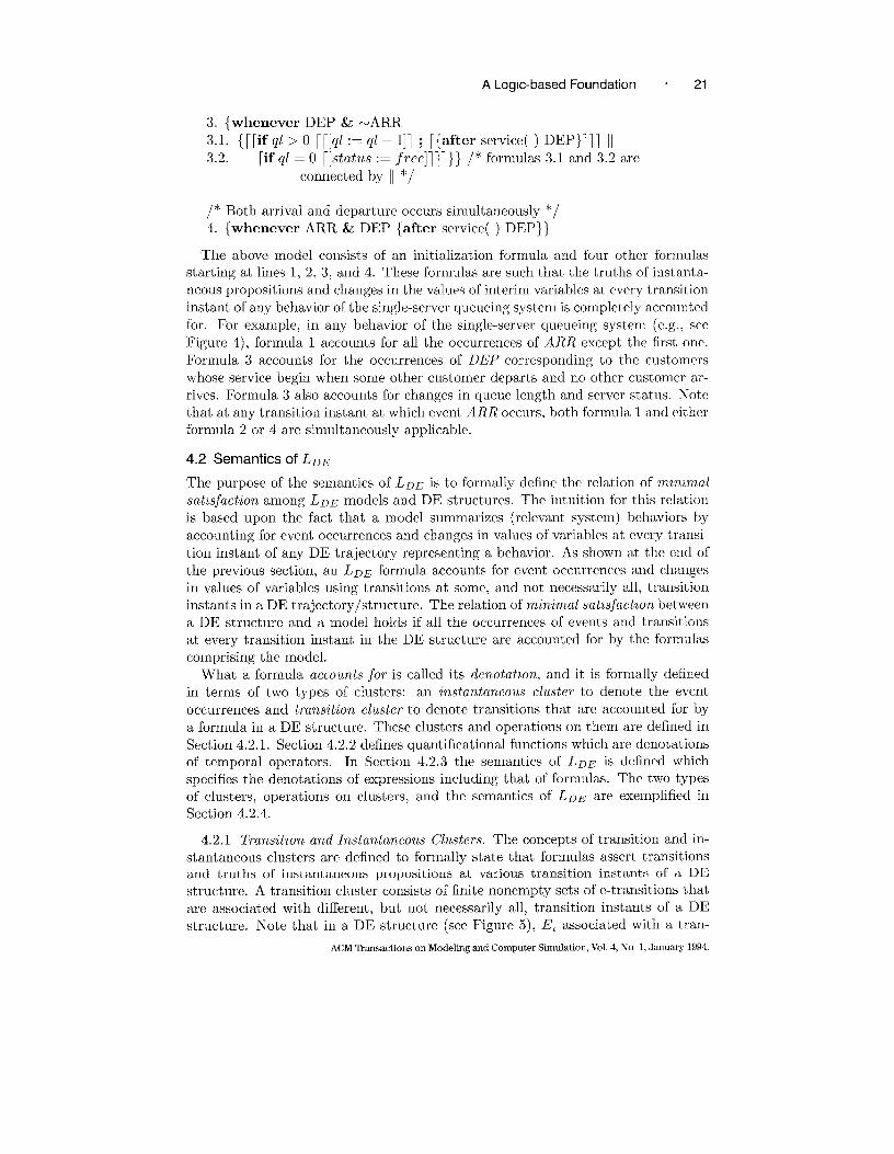
3. {whenever DEP & wARR
3.1. {[[if ql >0 [([q/ := ql – 1]1 ; [{after service( ) DEP}lll II
3.2. [if ql = O [[status := free]lll }} /* formulas 3.1 and 3.2 are
connected by II */
/* Both arrival and departure occurs simultaneously*/
4. {whenever ARR & DEP {after service( ) DEP}}
The above model consists of an initialization formula and four other formulas
starting at lines 1, 2, 3, and 4. These formulas are such that the truths of instanta-
neous propositions and changes in the values of interim variables at every transition
instant of any behavior of the single-server- queucing system is completely accounted
for. For example, in any behavior of the single-server queueing system (e.g., sce
Figure 4), formula 1 accounts for all the occurrences of ARR except the first one.
Formula 3 accounts for the occurrences of DEP corresponding to the customers
whose service begin when some other customer departs and no other customer ar-
rives. Formula 3 also accounts for changes in queue length and server stat 11s. Not c
that at any transition instant at which event ARR occurs, both formula 1 and either
formula 2 or 4 are simultaneously applicable.
4.2 Semantics of LDE
The purpose of the semantics of LDE is to formally define the relation of mtn7mal
satzsjaction among LDE models and DE structures. The intuition for this rclatiou
is based upon the fact that a model slunmarizes (relevant system) behaviors by
accounting for event occurrences and changes in values of variables at ever,y transi-
tion instant of any DE trajectory representing a behavior. As shown at the end of
the previous section, an LDE formula accounts for event occurrences and changes
in values of variables using transitions at some, and not necessarily all, transition
instants in a DE trajectory/structure. The relation of minimal satzsfactzon between
a DE structure and a model holds if all the occurrences of events and transitions
at every transition instant in the DE structure are accounted for by the formulas
comprising the model.
What a formula accounts for is called its denotation, and it is formally defined
in terms of two types of clusters: an instantaneous cluster to denote the event
occurrences and transition cluster to denote transitions that are accounted for by
a formula in a DE structure. These clusters and operations on them are defined in
Section 4.2.1. Section 4.2.2 defines quantificational functions which are denotations
of temporal operators. In Section 4.2.3 the semantics of LDE is defined which
specifies the denotations of expressions including that of formulas. The two types
of clusters, operations on clusters, and the semantics of LDE are exemplified in
Section 4.2.4.
4.2.1 Transition and Instantaneous Clusters. The concepts of transition and in-
stantaneous clusters are defined to formally state that formulas assert transitions
and truths of instantaneous propositions at various transition instantfi of a DE
structure. A transition cluster consists of finite nonempty sets of e-transitions that
are associated wit h different, but not necessarily all, transition instants of a DE
structure. Note that in a DE structure (see Figure 5), E, associated with a tran-
ACM Transactions on Modeling and Computer Simulation, Vol. 4, No 1, January 1994.
22 “ A Radlya and R. G. Sargent
sition instant I is a finite nonempty set of (:-transitions. A transition clllstcr is
formally defined to be a sl~bset of N x ~TE. Similarly. an instantaneous cluster is
defined to be a subset of N x ~ to assert noncmpty sets of propositions that are
true at different transition instants of a DE structure.
Definztzon. A trunsltLon cluster tc is a subset of (N x IITE ) such that (1) (Yn : rl ●
N) [if (7L, E) G tc then E is nunempty and finite] and (’2) (Vrr : n ~ N) [there MC
finitc!ly’ many tllples (T?,. -) with the same TL in tc].A transition clluiter is denoted
by tc,possibly with a numerical subscript, and the set of all transition clusters by
TC
Definztmrr. An Lnstwntarzeous ctwster 7C is a subset of (N x ~) such that (1)
(’do : n E N)[if (n, d) c ic then ; is nonempty] and (2) (W, : n 6 N)[there arc
finitely many tuples (n. -) with the same n in ic]. AI1 instantaneous cluster is
denoted by LC, possibly with a numerical subscript, and the set of all instant anco~w
clusters by lC.
In the semantics of LD~, the following operations of compaction, translation,
and mar on clusters are needed because clusters denoted by a formula ,f of the
form {op jl }, {,fl II ,fz }, or { ,fl ; jz } arc obtained by combining clusters denoted
by formulas occurring in j. Now. more than one tuplc of the form (n, -), for a
pa~ticula,r n, can occur in a transition or instantancolls cluster. It is luwful to
“compact” a cluster so that it has at most one tuple (n, -) for each n. Then. a
transition cluster can be easily compared with an {,-transition, and an instantaneous
cluster can be compared with instantaneous ~’aluations in a DE structure. The
compaction operation combines a set of clusters into a single compactrd clllster. In
the definitions given below, the symbol ztcis used for a cllwter when the cl~uiter
can be either a transition cluster or an instantaneous clllster.
De,fiwitLon. A transition or instantaneous cluster ltr is compacted if (Vn : 71 ●
N) [there exists at most one (n, _) ● Ltc].
De,fin7tlon. Compaction opm-at~on w : IIIC + Ic, and M : lTTC + T~ is defkcd
as follows. Let .X” G IIIC or A“ c HTC. WX = {(n, l’) I n ~ N, (=itc : itc G .X”) [(n,
.) G ~tc], and Y = u {Y”’ I (n, Y’) E itc’ ~ Y}}.
The following translation opcrat,ion @ translates a cluster by n instants. It incre-
ments an instant referenced in each tuplc by n. The operation of mrm returns the
maximum transition instant referenced in a cluster. These operations are uscfld in
defining the scmant ics of {OU j’1 }. {f, ; ,fz }. [iop a,t, 1. and [n.fI : cr,t~l.
De,fin’Ltwn,. Operation %: N x (IC U Tr ) ~ (IC U TC ) is defined as follows. Let
itc E (1, u TC). $j(rj,itc) = 7LT itc = {(i + n, Y) I /, E N and (z, Y) c ztc},
De,fin ition. operation mar : (IC U Tc) - Nu{- 1, W} is defined as follows. Let
LtC ● (Ic U TC).
{
–1 if 7tc= O
mur(itc) = IL if (r~, -) ● itc and (~m : m E N) [n < ?n and (m. -) E itc]
cm otherwise
ACM Transactions cm Modehng and Computer Slmulalwn, trol 4, NO 1, Janu~ 199.I
ALogic-based Foundation - 23
The operations of H, @, or max are extended to any cross product of Ic and Tc by
applying the operation on to each component of the cross product. For example,
if X E II(TC x (IC x Tc)), then kJX returns (tc, (it, tc’))E (Tc x (lC x TC)),
where k is the compaction of the set {prl (prz (z) ) I x ● X} of instantaneous
clusters (similarly for t c and tc’). The operation of mar returns the maximum
over all of its components. Finally, the following relation of equivalence between
transition clusters and e-transitions is needed to formally define the relation of
minimal satisfaction.
Definition. Let tc be a transition cluster and e be an e-transition. tcE e iff {(i,
e(i)) I O g i < Iel} = &J{tc}.
4.2.2 Quantification Functtons. In the semantics of LDE, temporal operators
denote quantificational functions. The following definition is similar to the defini-
tion of quantificational flmctions given in Brown [1984] and Barwise and cooper
[1981] except that the domain of our function is (IIN x IIN) rather than IIN. This
is because LD~ is a kind of modal logic, and an additional IIN in the domain
contains information about the modality of DE structures, i.e., a set of transition
instants (see R3 in the next section). In the generalized quantifiers logic defined in
Brown and Barwisc and Cooper, quantifiers are nontemporal.
Defin~tum. A quantzjicatto?Lal f~Lnctton qf for N is a partial function of type
HN x IIN -P IIIIN satisfying conditions (1) q,f(x, y) is defined for every y ~ r C
N and (2) if q,f(:c, y) is defined then qf(~, ~) E Hllr. The set of all quantificational
functions for N is denoted by QF.
The operators next, if, when, whenever, unless, some, until, while, and
at denote quantificational functions next, i~ when, whenever, unless, some, untiil,
while, and at,respectively (see Appendix B).
4.2.3 Semanttc Rules. The semantics of LD~ is defined using the approach of
model-theoretic semantics [Dowty et al. 1981] which is the most common approach
of defining mathematical lo,gics. (The meanings of the term model in DELIS and
logics are orthogonal. In this article, the term model always connotes what is
meant by it in the field of DEMS except in the phrase “model-theoretic”, which
can be considered to bc a name for an approach to defining semantics. See Dowty
et al. for a historical perspective on the phrase model-theoretic.) The crux of the
model-theoretic approach is that the semantic value of a composite expression is
determined in a fixed way by combining the semantic values of its sub expressions.
This implies that the semantic value of every expression in a language is completely
determined by the semantic values of certain expressions called basic expressions
[Dowty et al.]. The model-theoretic semantics of a langl~age is defined by specifying
a mathematical structlu-e which defines semantic values of basic expressions and
an interpretation function [ ] which defines the semantic values of the remaining
expressions with respect to the structure.
The model-theoretic semantics of LDE defined below is more complex than the
semantics of the commonly usecl simulation languages, procedural programming
languages, and mathematical logics such as first order predicate logic or temporal
logics [Kroger 1987]. This complexity is primarily due to the nature of the compu-
tations specified by models in DEMS languages. Also, the constructs of LD~ that
ACM Transactions on Modeling and Computer Simulation, Vol. 4, No 1, Jwmmry 1994

24 . A, Radiya and R. G. Sargent
DE structure K
.0 i-1 i i+]
T$+$b
~o ~1 6,. , i5,+,~1 ~i+2
. . . . . .
% ~,-1 a, ‘JI+l
E. El-l E, E(
,+1.,. ) . . . ../---’.,-- . . ...---.a.- . ..%to ...’-----”’ ff - 1 11 ..,, f ,
..::.#-----r,---- . . . .
~../- --- ..,,
..~.-~-<-~ expansion of a nonempty and nonsimple e-transition------
. . .\
LDI structure D
o-
%’
:O’D... .$: ● ** +:;::; 3
6[)of D = 5, of K,n=lD1-1
Fig. 6. A DI structure D corresponding to a nonempty e-transition in a DE structure K
are not available in DEMS languages contribllte to this complexity. computations
in DEhIS languages consist of transitions which are applied either at the “global” or
“local” levels. Transitions at the global level are associated with clock time which
can be referenced directly b,y using the clock variable or indirectly by using con-
ditions on instantaneous propositions and interim variables. Local computations
on the other hand consist of possibly complex transitions at individual transition
instants of a DE structure. The computations at both levels are expressed using
operators sl~ch as whenever, while, until, if, and unless. This makes the formal
definition of LD~, and DEMS languages in general, more complex than most non-
simulation languages and mathematical logics. In designing a DEMS language it is
important to distinguish the global and local computations in the syntax and se-
mantics of the language. In the syntax of LDE, global computations are expressed
using formulas, and local computations are expressed using action-formulas and
transition-terms. At the semantic level, ‘LDI structures” capture the local conlpu-
tations and arc defined to be substructlues of DE structures as follows,
Defirutmn. A Discrete (DI) .str?Lcture is a tuple (iTo, e), where @[) E E is the
initial interim valuation, and e ● TE is a non-simple e-transition, such that e is
well-defined for a..
For a DI structure D = (6., e) and L : 0 s i < Iel, El and tiz+l arc defined as
E, = e(i) and if E, = {e I,..., en}, n > 1,then 0,+1 = 6,(UlSJ~~ {Eli}).
The transdzon znstants of D are the positions in list e and are represented by
interval [0, Icl ). The cardinality of D is defined as ID I = Iel, and it represents
the total number of transition instants in D. A DE structure contains many DI
structures. For any non-simple e-transition e occurring at a transition instant L of a
DE structure K, the DI structure D = (6,, e) is said to occur at i of K (see Figure 6).
The DI structures arc similar to DE structures except that the clock time and
ACM Tmnsactlons on Modeling and Computer Smudatlon, VOI 4, No 1, January 1994,
ALoglc-based Foundation “ 25
instantaneous propositions are not included. Hence, in the pictorial representation
of DI structures, the triangles corresponding to instantaneous valuations and the
clock times are absent. An interim vall~ation is represented in a DI structure by an
oval at a transition instant rather than ~ because the concept of real time is not
relevant in DI structures.
Now, in the semantics of LDE, global and local level compl~tations are distin-
guished by defining (1) the semantic values of terms, conditions, operator-phrases,
and formulas at a transition instant i of the DE structure K and (2) the semantic
values of terms, interim-conditions. interim-operator-phrases, transition-terms, and
action-formulas at a transition instant j of a DI structure D at a transition instant
z of the DE structure K (see Figure 6). (This is similar to the way in which the
semantics of temporal logics is defined with respect to a reference point in a W-ipke
structln-e [Krogcr 1987].) For an expression a and O s i < IK 1, [a]~’ denotes the
semantic value of o at transition instant i of K and [a] K, ~,11.j denotes the scmantiC
value of a at j of D of i of K. The superscripts K,i and K, z,D,j are omitted if
the semantic value of an expression does not change with the transition instants or
is independent of DE and DI structures. The semantic values of constants, func-
tion symbols. relation symbols, and p-transition symbols do not change with the
transition instants of a DE or DI structure. The semantic values of temporal opcr-
at ors, propositional connect ives, parallel connective, and sequential connective are
independent of the DE and DI strl~ctures. Function [ ] explicitly specifies semantic
values of constants ( [const] ~ Vai), function symbols ([g] E Valm - Val ), relation
symbols ([r] ~ Valm), instantaneous proposition symbols (~] E F’), and operators
([o] ~ QI’).
In the following, onc semantic rule is defined for each syntactic rule defined in
the syntax of LDE. These rules are illustrated in the next Section. As in the
syntax of LDE, o, c, tc, in,c, op, iop, tt, CLf, and t denote an expression of the
category operator, condition, t imecl-condit ion, interim-condition, opm-at or-phrase,
interim-operator-phrase, transit ion-term, action-formula, and formula. respect ivcl y.
Recall that b,, ~,, E,, t, refer to instantaneous valuation, interim valuation, a set
of e-transitions, and clock time at transition instant i of a DE structure K over
an interval 11 respectively (see Figure 6). The notation of representing an interim
valuation by a (possibly) subscripted @ is the same for DE and DI structures. In
the following semantic rules, unless specified otherwise, D, is t hc interim valuation
at transition instant i of K and 6J is the interim valuation at the jth transition
instant of the DI structure D at i of K.
Rules for defining semantic values of expressions
RO. [o] ~ QF
RI. 1. [const]h-” = [const]
[const]~’”~” = [conSt]
RI.2. [v]K” = 67,(V)
[V] K’” DJ = al (v)
ACM Transactions on Modeling and Computer Smmlatlon, Vol 4, No. 1, January 1994

26 . A. Radiya and R. G. Sargent
R1.3. [f(tel ,... ,te~)]k-’ = [,f]([te~]~-’, . . . . [ter~]~-”)
[.f(tel, . ,te~,)]h-’”~” = [f]([te~]K’l~J, . . . . [tc~]Kz~J)
R2. [(] K-’ = IH?+, [inC]R-’DJ E IIN
R2.1. [p] ‘z = {t,, I n >7 aucl ~] is t in 6,, of K}
R2.2. ~r(tel,.. .,te~)]fi”’ = {t I t E It 2 t, and ([tel]h-r’,. . [te,~]Kr’) E [~1.where n is such that t < f,,and if t.,_1 exists. t~, _ 1 < t}
[r(te~, .te~)]k” ‘D’ = {n I IDI > n ~ j and
([tel]~-’~’”,....[tf?n,]h-’’’~’”)E [7-]}
R2. Y. [N cl] ~’ = I ~’1 [tot,) e [cl]~”
[N inc~]~-’~j = [0, IDI) @ [O, j) e [inC,]K’~IJ
R,z~. [cl & ~~]KJ = [cl] R-L n [cz]k-’
[InCl & 7n,C2]KI’~J = ~LTLCl]~’DJ n [LTlc2]~zD.I
R,2.5. [tc]~” = {t I t > t, and tcevaluates to t by assuming the value of clock
to be t and current .time( ) to be t,}
R3. [op]h’ z, [iop]h-’’J’J E IIHN
[0 C]k-” = [0]([0, IKI – i), S) is defined iff (Vt : t E [C] K’)[(% : n >
~)[tJ of K = t]] and S = {n – i I n z i and t~ E [c]~’}
NOTE : The semantic value of [op] ~‘ is defined iff the set [c] 1{’ is a
denurnerable set such that all the elements of it are the times of transition
instants of K.
[o inc]h-2DJ = [0]([0, IDI -j), S), where S = {n -J I n ~ [inC]~’DI }
R~. [tt]A-’z E (TE X (~~ X T~Y))
R4.1. [[v := tr]]K’D] = (({P}), (0 0)) is defined iff ({p}) E EJ of D. where
~) E TP such that p(m) = {~/uai} and ~d is the value of term te in
intmim valuation tiJ
R4.2. [[af]]KzDJ = (e, (it, tc)) is defined iff 3e E EJ of D sllch that (tcl, (it, tc))
= [~L,f]Co is defined, where DI structure G = (tiJ of D, e). and c = tcl
R5. [cj]~’DJ E (Tr X (~~, X TC))
R5.1. [(ttl]K’D ‘ = ({(0, {TWl([tt]K’ ~’)})}, IJrZ([tt]h”’DJ,)) is defined iff
[tt]k ‘ DJ is defined
R(5.2. [~~0~ afll]A’’DIJ = (ti{?l @ ~~l([a,fl]A-i’’DJ+ ’L) I n G z},
M{m2([f/fl] ‘LIDI’+n) I rL c z}) is defined iff 3Z ● [ZOP]R-’DIJ and
(Vn : n E :)[[(t,f,] ~l’D1+r’ is defined]
R5.3. [[afl II c~,f21]~-’D ‘ = U{[afl]~’~)J, [c~fj]H’’D’} is defhled iff
[of,] ‘-’D*J and [afz]KtD) are defined
R5.4. [[f~jl ; afzl]R”21JJ = &J{[afl]K ‘D’, ((1+ n)&prl([a,fz]R’’’JJ+l+”),
prz ( [a,f~] ‘-’DJ+’+n) )} is define~l iff [~~fl]k-’DJ and [a~2]h’zD~+’+~ are
defined, where n = rnax(pr-l ( [afl] ‘“’DJ ) )
R5.5. [ [fl]K’DJ = (@, [f] ‘{’) is defined iff [~]~’ is defined
R6. [f]K’ c (IC X TC)
ACM ‘Ikinsactmns on Nlodelmg and Computer Slmulatmn, Vol 4, No 1, January 1994

ALogic-based Foundation o 27
Rtl.1. [{af}]A-” =(iC, bJ{{((), {e})}, tc})isdefined ifl~e~~, ~fK~~Ch that
(tc, , (it, tc)) = [af] ~,~~o is defined, where DI structure D = (5, of K,
e), and e~tcl
R6.2. [{Op~l}]K-’=M{rt@[~l]R-Z+n ln~~}isdefinediff~z~ [op]~,~ ~Ild
(’dn : n E Z)[[f,] ~“+n is defined]
R6.3. [{f, 11.f2}]A-’L =w{[fllK”1 [~z]~-’} is defined iff [~1]~’ and [fz]~-’ arc
defined
R6.4. [{fl;fz}]~’ = ~{[~l]k-’, (1 +n) @ [F.]~’’+l+”} is defined iff [j’l]~’ and
[~z]k’’+l+n are defined, where n = rrum( [~1] ~’)
R6.5. [{p}]~’ = ({(O, {[p]})}, ~) is defined iff ~j] is t in b,
R 7. Let a model T = {fl,. . . . f., } he a finite set of formulas. A DE structure K
= (H, X) mmimally satzsjies T, written as K \ T, iff
(1) (Vi :1 s i ~ rn)[ [~,]~’o is defined],
(~) {(n, X(n)) I O < n < IKI} = &{prz([,fz]A->o) I 1 s i s m}, and
(3) (~n :0 s n < lKl)[tin of K = (if (n, S) is defined in U{p-l([~,]~O) ] 1< i s m}
then S else ~)].
The above definition of the semantics of LD~ can be applied to decide whether
an arbitrary DE structure satisfies a given model. A DE structure is said to satisfy
a model if the semantic values of the formulas of the model are defined ((1) of R 7)
and all the occurrences of the instantaneous propositions ( (3) of R 7) and transitions
((2) of R?’) in that DE structure are completely accounted for. If a DE structure
dots not satisfy a model then either some expressions occurring in the model are
not clcfined, or all the occurrences of instantaneous propositions and transitions
in that DE structure are not accounted for by the formulas of the model. In the
remainder of this article, (italicized) Rn. m refers to a semantic rule given above.
Recall that Rn.m refers to a syntactic rule.
4.2.4 E:mmplificat70n of Semantics. The semantics of LD~ is cxcrnplified by
defining the semantic value of formula F3 (lines 3, 3.1, 3.’2) in the model of the
single-server queucing system in Section 4.1 with respect to the DE structure K
over the interval 1 shown in Figure 5. The semantic value of F~ formally specifies
what is accouutcd by it in K. Intuitively, by examining ~3 and K, it can be noted
that F3 accounts for certain occurrences of DEP such as at transition instant 3 but
not at transition instant i + 1, and e-transitions such as e~ at transition instant 2
and el at transition instant 3. In LDE, the semantic value of a composite expression
such as F3 is defined using the semantic values of its sub expressions. For defining
the semantic vallw of F3 at transition instant O of K it is necessary to define the
semantic values of some of its subexpressions with respect to DI structures. For
the purpose of this illustration, the semantic valllcs of some sub-expressions of F3
are defined at a transition instant (J of DI structure D = (ti2, ({ ({ fJ.2}) }) ) occurring
at transition instant 2 of K (see Figure 7). The semantic vallles of ~j and its
sllbexpressions are given in Table 1. Each row in the table consists of six entries:
(1) row number, (2) an expression e.rp, (3) i to mean the transition instant i in DE
structure K or i, j to mean the transition instant j in DI structure D at i of K,
(4) semantic value [erp]k-’ or [ezp]~>’DJ, (5) semantic rules used for defining the
ACM Transactions on Modeling and Computer Simulation, Vol 4, No. 1, January 1994
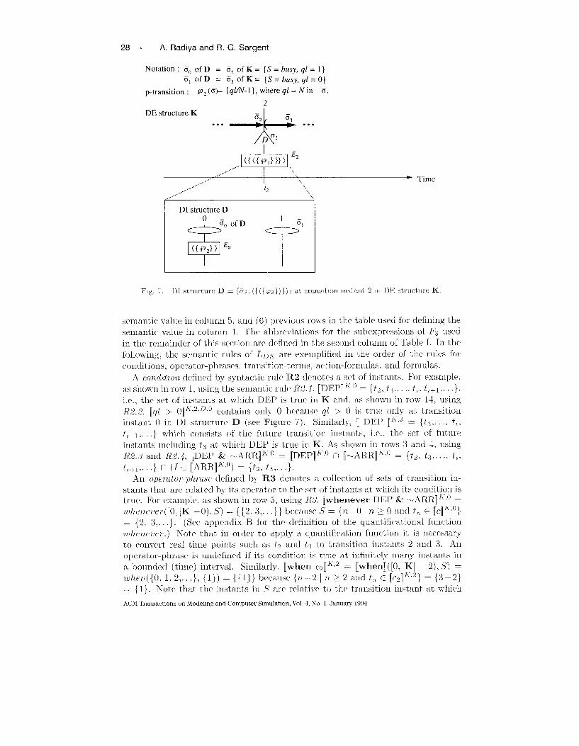
28 . A. Radiya and R, G, Sargent
Notation : 60 of D = 62 of K= {S= busy, ql = 1]
6} of D = 6~of K= {,S=busy, ql=O]
~.tran~ition ; jo2 (6)= (q//N-1 ), where ql = N in 6
2
DE structure K
. . . A . . .
Ez({({; 2})})
.-+”.,, ‘\.<-. +..,’ I \ Time
---,.- 12 \\, ,.-” \
DI structure D
o~(, of D
1-
“F “T
~!
({@,}) ‘“
Fig. 7. DI strllcturc D = (62. ({({ pZ }) }) ) at transition instant 2 ]n DE structure K
semantic value in collunn 5, and (6) prc~ious rows in the table used for defining the
semantic vallw in column 4. The abbreviations for the subcxprmsions ot FS used
in the remai~ldcr of this section are defined in the second collmm of Table I. In the
following, the semantic rules of LD ~ are exemplified in the order of the rides for
conditions, operator-phrases, transition-terms, action-formulas. and formulas.
A condhon defmcd by syntactic rldc FL2 denotes a set of instants. For example,
as shown in row 1, luiing the semantic rule R2. 1, [DEP]~’) = {tj, t~.. . . t,. t,+l,. . .},
i.e., the set of instants at which DEP is true in K and, as shown in row 14, using
R2.2. [q/ > (j]~.~D,O contains OHIY O because ql > 0 is true only- at transition
instant () in DI structlm> D (see Figure 7). Similarly, [ DEP ]~3 = {t:j,. . . . t,,
t,+l,...}whirh consists of the fl~trn-e transition instants, i.e., the set of future
instants incllding ts at which DEP is true in K. As shuwn in rows 3 and -1, using
R2. # and R2.4, [DEP & WARR]h” 0 = [DEP]k-O n [wARR]h-O = {t2, t3,. . . . t,,
t,+~,...}fl(1:)[ARR]k’(’) = {t?, t,j,...}.
An operator-phrase (Iefined by R3 denotes a collection of sets of transition im
stauts th:lt arc related by its operator to the set (Jf instants at which its condition is
t rl~e. For example: as shown in row 5, using R3, [whenever DEP & wARR] ‘“0 =
/lj//c/l,(./,er([(), IKI –()), S) = {{2. :3,. . .}} becal~se S = {?~—O I n ~ O aIl(l tn 6 [C]l<O}
= {2, 3,...}. (See appcnclix B for the (ldinitiorl of the quantifkational function
,(h~ru,,rr.) Note that in m,icr to apply a quantification function it is ~~ecessary
to convert real time points sllch as tz and t~ to transition iustants 2 and 3. An
operator-phrase is undefined if its condition is trlle at infinitely many instants in
a bolmrled (time) interval. Similarly [when CZ] ‘“2 = [when] ( [0, IK I – 2), S) =
when({O, 1, 2,.. .}, {l}) = {{l}} brcaluw {7/–2 I n >2 and t,, ~ [C2]A-2} = {3–2}
= {1}. Not{: that the instants in S are relative to the transition instant at which
AChl Transwtlons on Modeling and Computer Slmulatlon, Vol 4, No 1, January 1994

ALogic-based Foundation “ 29
Table I. Semantic values of expressions
structure D shown in Figures 5 and 7.
#
1~
34
5
6
7
8
9
10111213141.516
17
18
19
20
21
Expression e.rp a
DEP
ARR
wARR
CI = DEP & eJARR
opI = whenever c1
Q E clock = C( )
I
2, 0
2,02,0
2.02.0
with respect to the DE structure K and DI
Semantic value
[eqI]K’, [e.zp]K,’~J
{t2, t~,..., t,, t,+,,...}{to, t,,..., t,, t,+,,...]I ~ [ARR]A’o
{tz,t,,.,.}{{2, 3, .}}
{t,}
{{l}}
({(m {~~~})} 4)
({(l) {~~f’})}, 4)
(4) ({(1 {~~p})}, 4))
(({m})! (d 0))({(0 {({w})})}. (4> d))({(Q {({f’2})})}. ({(1, {DEP})}, 4)){0}~{o}}({(Q {({ KJ2})})} ({(1, {~~p})}i 4))
[{(0 {({ku})})}! ({(1({(1, {~~p})}l {(a {
(0, {(0 {({w})})})({(3. {DEP}),. .},
{(21 {({ P2})}) (3
{DEW})}, d))[pz})})})
({FI})})V.})
Rules ‘
R2. 1R2. 1
R2. 3R2.4
R3
RI 2R2. 5
R3
R6.5
R6.2
R5 5R4.1R5 1
R5.4R2.212:1
R5.2R2.2,.5R.5.2Rc5.3
R6. 1
R6.1
R6.2
Rows d
2
1,34
6
7, 8
9
11
10, 12
14
13
16, 17
18
5, 20
“c( ) = currellt-tim~( ) = tz, c( ) + S( ) = tz + service.time( ) = f3‘For each row, the sernantlc value of eJ v is defined at transition instant K, z or K. T. D, I
CApplicahlc semantic rides
,.
‘iSemantic values frum these rows in the table are used for the clu-rent row
an operator-phrase is evaluated. Similarly, row 15 defines the semantic value of an
interin-operator-phrase.
A transLtLo71-term defined }y R4 clcnotes an element (c, (it, tc)) E (TE x (~e x
Tr)), where e is an e-transition occurring at the transition instant ~ of D at i of K,
and (it, tc) is a pair of instantaneous and transition clusters denoted by formldas
(dcfmcd by R6) occlu-ring, if’ any, in the transition-term. For example, as shown in
row 11, lwing R~. 1, [[qt := ql — I]] ‘-2$ D>” = ( ({ fJ2}), (~, ~)), where p-transition p~
(defined in Figure 7) corresponds to ql := ql -1. Note that (it, tc) = (@, ~) because
no formulas are contained in [ql := ql — 1].The semantic rule R4. 2 is similar to
R6. 1, which is exemplified below.
An m:tiLun-,formulu, ddinecl by R5 denotes an element (tcl, (k, tc) ) E (TC x (lC x
TC ) ), where tcl is a transition cluster relative to j of D at i of K, and the intcrprc-
t ation of ( ic, fc) is the same as that for the transitioll-terms, For example, as shown
in row 12; using R,5.1, [[[qi := ql – l]]]~z~o = ({(0, {({h~~})})}, (j, d)), where{(0, { ({ fJ~}) })} is a transition cluster. Hence, an action-fornnda defined by R5. 1
ACM ‘Ikanstactmns cm Modehng and Computer Siiulatlon, Vol 4, No 1, January 1!394
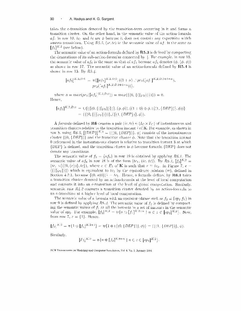
30 “ A. Radlya and R. G. Sargent
takes the e-transition denoted by the transition-term occlu-ring in it and forms a
transition cluster. On the other hand, in the semantic vallw of the actiomformula
a,fl in row 10. tcl and tc are @ because it does not contain any expression which
asserts transitions. Using R5. 5, (~c, tc) in the semantic value of afl is the same as
[f,]~’z (see below).
The semantic value of an actiomformula defined by R5.3 is defined by compacting
the denotations of its sub- actiomformulas connected by II. For example. in row 18,
the semantic vall~c of (~~h is the same as that of a,f.i becal~se af5 denotes (@, (~. o))
as shown in row 17. The semantic value of an action-formula defined by R5.4 is
shown in row 13. By R5.4.
[af3]A->2,D,II
= u{({(()> {({ f~2})})}!( 4,@))> ((l +0) @$k({(l. {~~~})}. @))}
= ({(o{ ({m}) })})({(1>{~ ~~})}>o)).
A ,forwLda defined by R6 denotes a pair (it. tc) E (IC x TC ) of instantaneolw and
transition clusters relative to the transition instant i of K. Fc)r example, as shown in
row 8, lwing R6. ,5, [{ DEP}] R 3 = ({(O, {DEP} ) }, @) consist,s of the instantaneous
cluster { ((), { DEP} ) } and the transition cluster ~. Note that the transition instant
O rcfcrcnccd in the instantaneous cluster is relative to transition instant 3 at which
{DEP } is defined, and the transition cluster is Q$because formula {DEP } does not
denote any transitions.
The semantic value of f~ ~ {a f6 } in row 19 is obtained by applying R6. 1. The
semantic value of af6 in row 18 is of the form (tcl. (it, tc)). By R6. 1, [f3]h-2 =
(it, w{{(O, {e})}, tc}), where e E E2 of K is sllch that e ~ tel. In Figure 7, e =
({ ({iu}) }) which is equivalent to tcl by the eqlli~-alcnce relatlon (=), defined in
Section 4.2.1, because {(0, e(0)) } = tcl. Hence, a forrnlda defined by R6. 1 takes
a transition cluster denoted by an actiomforrnlda at, the level of local computation
and converts it into an e-transition at the level of global compl~tation. Similarly,
scmant ic rule R4. 2 converts a transition cluster denoted by an action-formula to
an e-transition at a higher lCVC1 of local computation.
The semantic vall~e of a formula with an operator-phrase such as ~z ~ {OPJ fl } in
row 9 is defined by applying R(7. 2. The semantic value of ,fi. is defined by conlpact-
ing the semantic values of ,fl at all the instants in a set of instants in the semantic
value of Opz. For example, [f2]K2 = W{7Z @ [fl] ‘-2+” I n E Q● [op2]K2}. NOW,
from row 7, z = {l}. Hence,
[,f,]~’ = kl{l+ [j,]~’’+’} = EkJ{l@ ({(0. {DEP})},45)} = ({(1, {DEP})}, 4)
ACM TransactIons on Modeling and Computer Slmulatlon, J’ol 4, No. 1, January 1994
A Logic-based Foundation “ 31
Now, from row 5, z = {2, 3,. . .}. Hence, as shown in row 21,
[F,]h->” = W{2 @ [f3]~-’o+~, 3 @ [f3]~’o+~, . . .}
= &J{2 @ ({(1, {mm})}, {(0, {({ fJ,})})}).
3@(q5, {(()> {({@} )})})$}
= ({(3, {DEP})}, {(? {({ KJ2})}), (3, {({6’1})}), . .}).
The semantic rules R6. 5’ and R6.4 are similar to semantic rules R5. 3 and R5.4,
respect ively.
The semantic value of F3 defined in row 21 formally states that the e-transition
({gJ,}) ad the occurrence of DEP at transition instant 3, and the e-transition
({P2}) at transition Instant 2 of K are accolmted for by it. Similarly, the denotata-tions of other formulas of the single-server model can be defincxl using the semantic
rules of LDE. The DE structure K shown in Figure .5 is said to minimally satisfy
the model if all the occurrences of instantaneous propositions and transitions in K
are accounted for by the formulas of the model.
5. MODELING USING LD~
In this section, the modeling constructs of L~~ are illustrated and compared with
those of ES WV languages by modeling a preemptive single-server queueing system.
As mentioned at the beginning of Section 4, the logic-based foundation views that
the purpose of the modeling constructs of DEh’IS langl~ages including ESWV lan-
guages and LD~ is to (1) refer to transition instants in a DE trajectory and (2)
assert occurrences of events and/or changes in the values of some variables at these
instants. The modeling constructs of LDE are formally defined by the syntax and
semantics of LDE given in Section 4.1 and Section 4.2.3, respectively. As explained
in Section 4.1, in LDE, transition instants can be referenced using ( 1 ) a logical con-
dition c on propositions, variables, and clock time and (2) an operator-phrase, o c,
which refers to a set of instants that are related by a temporal operator o to the set
of instants at which condition c is true. The occurrences of events and/or changes
in values of variables using transitions can be asserted using formulas of the forms
{o c ~1 }. {~1 II ~z }, {.fl ; .f2}, and {P}. where f, is a formula and p is an instan-taneous proposition symbol. The intuitive meaning of these constructs is given in
Section 4.1, and the working of these constrl~cts is exemplified in Section 4.2.4.
The preemptive single-server queueing system that is modeled in this section
consists of one server which serves hot h the high- and low-priority cl~st omers. A
high-priority customer preempts a low-priority cllstomer. A preempted cllstomer’s
service begins all over again when all high-priority customers in the system have
been served. It is assumed that only one customer arrives at a time. Three rnodcls
are presented: an ESWV model which utilizes priority and cancellation constructs, a
simple L~~ model which utilizes logical combinations of events and a new temporal
operator unless, and an alternate LDE model which utilizes logical conditions on
events and interim variables in more sophisticated ways and the parallel connective
Il. Them modek arc confitructed u.ing the mme events, variablm, and functions
which are as follows.
E~lents or instantaneous propositions:
ACM Transactions on Modehng and Computer Simulation, \’oI. 4, No. 1, January 1994

32 “ A, Radiya and R. G. Sargent
(1) HP~A — High-Priority Chstomer Arrives
(2) LPCA -- Low-Priority Customer Arrives
(3) DEP — DEParture of a low- or highpriority customer
Irlter7m Vurlables:
(1) status: {busy-high, tmsy.lou, free} — statl~s of the server
(2) ql.hzgh: N — length of the queue of high-priority cl~stomers
(3) ql.lou: N — length of the queue of low-priority cl~stomers
(4) temp: R+ — a variable to store temporary values
Functions:
(1) intcrarrival( ): R+ — A function for interarrival times of cluitomcrs
(~) servicc( ), R+ — A f~m~ti~n for the serl,ice times of customers
(3) type( ): {h/gh, low} — A function for the type of the next customer
In simulation languages based on ESVVV, as mentioned in Section 1. a model
consists of a set of event routiues. The execution of an event rolltmc may change
vall~es of some variables and may schedule or cancel events in the future or at the
present time. The event routines of simultaneously occlu-ring events are execl~td
sequentially in the order determined by the priorities given to the event routines.
The following ESWV model consists of three event routines HP~A, LP~A, and
DEP (their priorities arc discussed below). In this model. when a low-priority
customer’s service begins, an instance of DEP marking the departure of the cus-
tomer is scheduled. Subsequently if a high-priority customer arrives while the
low-priority customer is still being served then the preemption of the low-priority
customer is achieved by incrementing ql-lou] by 1 and canceling the imstance of
DEP that was scheduled earlier. The following model is defined in the pseudo syn-
tax which resembles ~ or PAS~AL-like languages. A statement of the form {after
real -expr eL)ent-name} means that an instance of event Fwwlt_71ame is scheduled
after real -e:zpr units of simulation time.
MODEL 1: An ESWIT model of the Preemptive Single-Server System.
/* Initialization statement */
1. {status := ,frce; ql.high := O; ql-lmo := O;
2. if (typc( ) = lngh) then {after intcrarrival( ) HPC’A}
else {after interarrival( ) LPCA} }
/* A function call t~pe[ ) returns high or low which is used to schedule
either HPCIA or T,PCA */
/“ Departure occlu-s “/
3. {event routine DEP
4. if (ql-high > O) then {ql.high := ql_high – 1; status :Z busy. h:?gh,;
{after service( ) DEP}}
5. else if (ql-low > O)
6. then {ql-low := ql-low – 1;status := busy -loul;
{after service( ) DEP}}
7. else status := free}
ACM Transactions cm Modehng and Computer S]mulatlon, Vol. 4, No 1, January 1994

ALogic-based Foundation “ 33
/“ A high-priority customer arrives “/
8. {event routine HPCA
9. if (type( ) = high) then {after interarrival( ) HPCA} else {after
interarrival( ) LPCA};
10. if (status = busy.high) then ql.high := ql_high + 1
11. else {if (status = busy-low) then {ql-low := ql-low + 1; {cancel
DEP}}; /* Insert a preempted customer in the low-priority
cutomers queue and remove the entry of DEP
from the future event list */
12. status := busy-high; {after service( ) DEP}}}
/“ A low-priority customer arrives “/
13. {event routine LPCA
14. if (typc( ) = high) then {after interarrival( ) HPCA} else {after
interarrival( ) LPCA};
15. if (status # free) then ql.low := ql-low + 1
16. else {status := busy-low; {after service( ) DEP}}}
Although, the priority mechanism has been found useful in modeling the situa-
tions in which the effects of simultaneously occurring events may depend on each
other, it is not cas y to correctly assign priorities to event routines. It is obvious
that LPCA should have the lowest priority. The event routine HPCA cannot have
higher priority than DEP becal~se this will preempt a low-priority customer that
is about to depart when HPCA and DEP occur together. Now, if DEP has higher
priority than HPCA then it causes unnecessary scheduling and cancellation of an
event when DEP and HPCA occur at the same time and, also, ql_high = O and
ql-low > 0. In this situation, DEP is processed first which starts the service of
a low-priority customer and schedules an instance of DEP. This newly scheduled
instance of DEP is immediately cancelled by the processing of HPCA. This problem
can be solved by using the information about the time at which the server will finish
serving a customer that is available in simulation but not in the real system. One
way to accomplish this in Model 1 is to use a separate variable, say extra, to store
the departure time of a low-priority customer; give the highest priority to HPCA;
and modify the code of HPCA to take into account a simultaneous occurrence of
DEP of a low-priority customer by examining extra. However, such a solution is
“unnatural” because the value of the variable extra is not available in the real sys-
t em. ( Zeigler [1976, p. 137] discusses disadvantages of using priorities and suggests
an alternative way of handling simultaneous event occurrences. )
It was discussed in Section 1 that operators whenever and when are implicit
in ESWV languages. It can be verified by examining the code of the above ESWV
model that an event routine which does not use the cancel construct syntactically
corresponds to an LDE formula of the form {whenever p {a~}}, where action-
formula a~ is restricted to [{when clock = real-expression {p} }1 I [ ttlI[ if ic a.fl
1 I [ a.fl ; a.fl 1. However, the semantics of the event routine is diflerent from the
corresponding LDE formula because priorities are assigned to event routines. The
logic LD~ does not have mechanisms for setting priorities or canceling events. The
ACM Transactions on Modeling and Computer Slmulatlon, Vol. 4, No. 1,January 1994
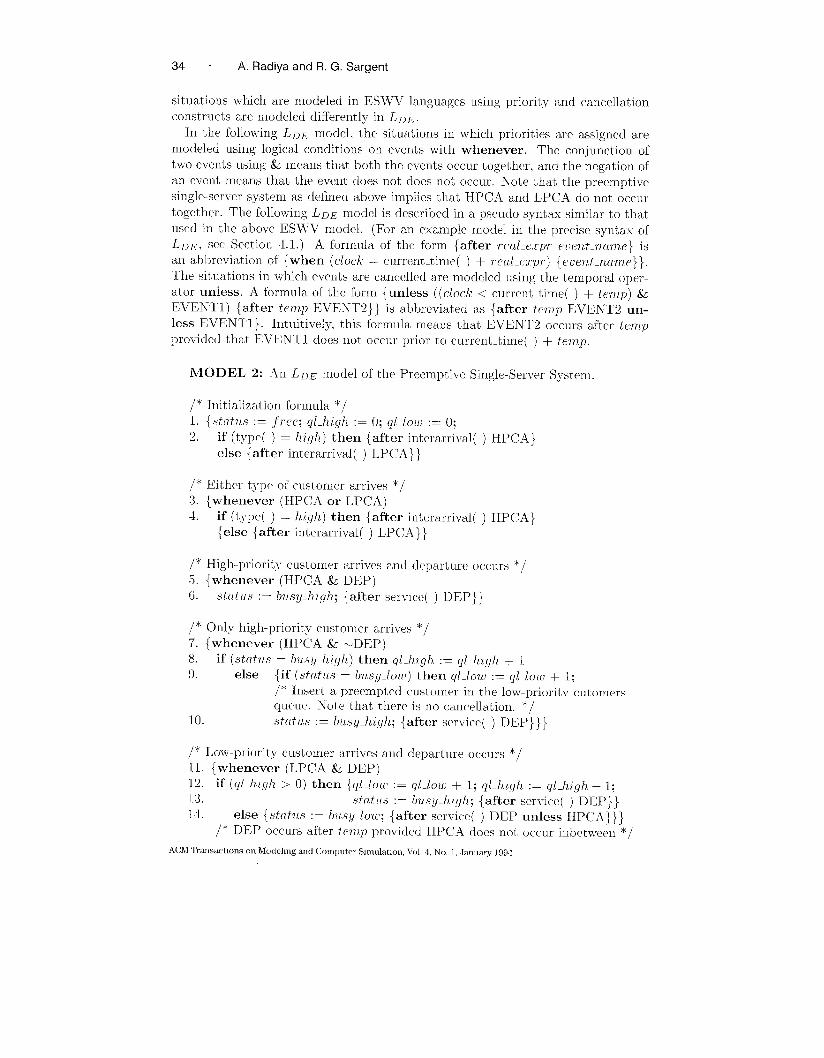
34 “ A. Radiya and R. G. Sargent
situations which are modeled in ESWV languages using priority and cancellation
constructs are modeled differently in LD~.
In the following LD~ model, the situations in which priorities are assigned are
modeled using logical conditions on events with whenever. The conjunction of
two events using & means that both the events occur together, and the negation of
an event means that the evcut does not does not occur. Note that the preemptive
single-server system as defined above implies that HPCA and LPCA do not occlu-
together. The following LDE model is described in a pseudo syntax similar to that
used in the above ESW’V model. (For an example model in the precise syntax of
L ~F, sce Section 4.1. ) A formlda of the form {after rral-e.rpr e~ent-nume} is
w abbreviation of {when (clock = current_time( ) + reul-ezyn-) {euen-n,mn,e} }.
The situations in which events are cancclled are modeled using the temporal oper-
at or unless. A formula of the form {unless ((clock < current -time( ) + temp) &
EVENT1 ) {after ternp EVENT2} } is abbreviated as {after temp EVENT2 un-
less EVENT1 }. Intuitively. this formula means that EVENT2 occurs after ternp
provided that 13VENT1 does not occur prior to current.time( ) + temp.
MODEL 2: .411 LD~ model of the Preemptive Single-Server System,
I*1.9-.
I*3.
4.
I*5.
6.
1“7.
8.
9.
10.
Initialization formula */
{stfItus := free; ql_high := O; ql.low := O;
if (typc( ) = high) then {after interarrival( ) HPC.4}
else {after interarrival( ) LPCA} }
Either type of customer arrives */
{whenever (HPCA or LPCA)
if (type( ) = high) then {after interarrival( ) HPCA}
{else {after intcrarrival( ) LPCA}}
High-priority customer arrives and departure occurs */
{whenever (HPCA & DEP)
stci,tus := hls~.h~,qh; {after servlcc( ) DEP}}
Only high-priority customer arrives */
{whenever (HPC’A & wDEP)
if (statl/s = bu.~~]_hiqh) then ql.fngh := ql-hzgh + 1
else {if (stat{~s = hI,s,y_/ou) then ql.low := ql.low + 1;
/* Insert a Preempted customer in the lowrrrioritv crrtorners
queue. Note that there is no cancellation. *I
status := bus,@gh; {after scrvice( ) DEP}} }
/* Low-pri~rit~ customer arrives and departlme occurs */11. {whenever (LPCA & DEP)
12. if (ql.h,t,yh > O) then {ql-lou, := ql.low + 1;ql-h~qh := ql-high – 1;
13. .stato.j := busy _hr,qh; {after serx,icc( ) DEP}}
14. else {statq~s := b~(,sy.lou,; {after servicc( ) DEP unless HPCA} } }
/“ DEP occurs after f~?~~p provided HPCA does not uccur inbctween “/
ACM TransactIons on Mwlehng and Computer Simulatmn, t’ol 4, No. 1, Januaw 1994
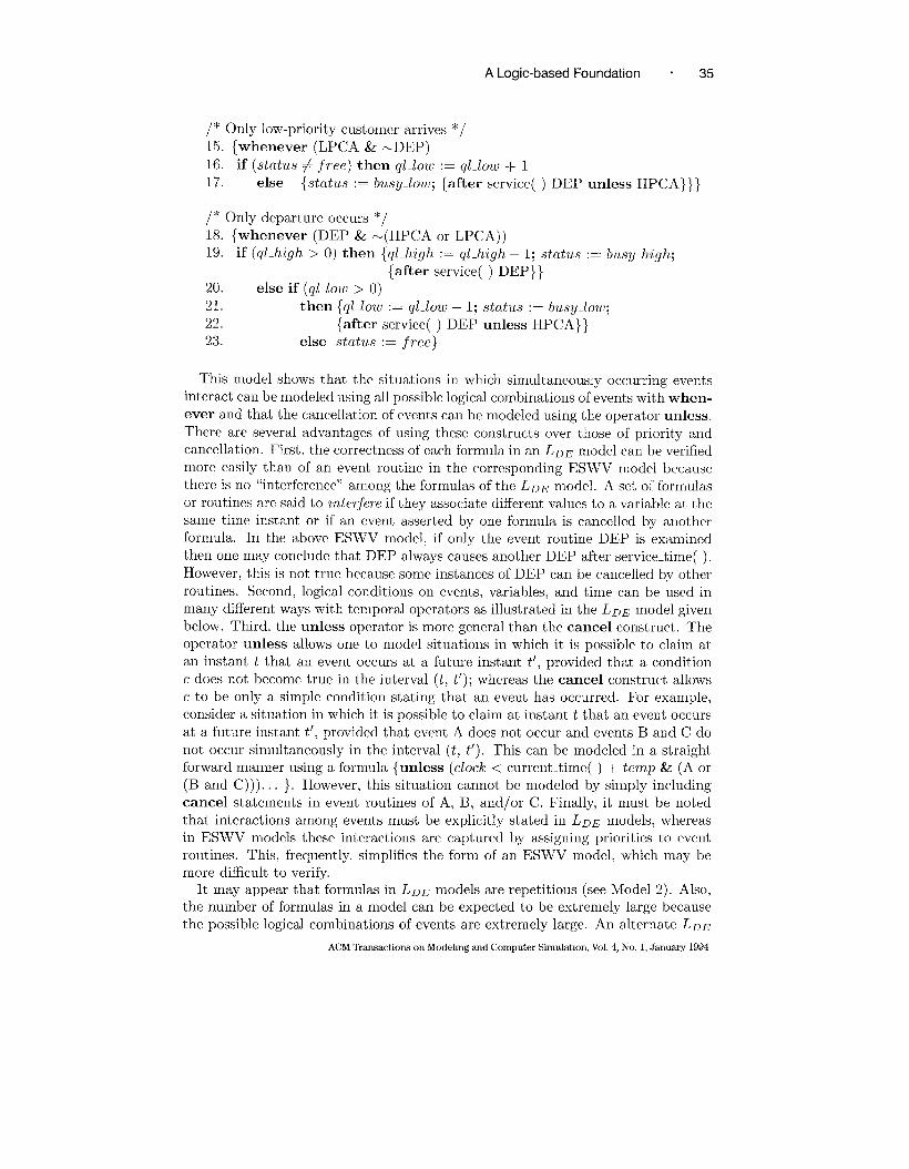
ALogic-based Foundation “ 35
/“ Only low-priority customer arrives “/
15. {whenever (LPCA & wDEP)
16. if (status # free) then ql.low := ql_low + 1
17. else {status := busy-low; {after servicc( ) DEP unless HPCA}}}
/“ Only departure occurs ‘/
18. {whenever (DEP & w(HPCA or LPCA))
19. if (ql.high > 0) then {ql-h,igh := ql_high – 1; status := busy _high;
{after service( ) DEP}}
20. else if (ql-low > O)
21. then {ql-low := ql-low – 1; status := busy.low;
22. {after service( ) DEP unless HPCA}}
23. else status := free}
This model shows that the situations in which simultaneously occurring events
interact can be modeled using all possible logical combinations of events with when-
ever and that the cancellation of events can be modeled using the operator unless.
There are several advantages of using these constructs over those of priority and
cancellation. First. the correctness of each formula in an LDE model can be verified
more easily than of an event routine in the corresponding ESWV model because
there is no “interference” among the formulas of the LDE model. A set of formulas
or routines are said to znterjere if they associate different values to a variable at the
same time instant or if an event asserted by one formula is cancclled by another
formula. In the above ESWV model, if only the event routine DEP is examined
then one may conclude that DEP always causes another DEP after service_time( ).
However, this is not true because some instances of DEP can be cancellecl by other
routines. Second, logical conditions on events, variables, and time can be used in
many different ways with temporal operators as illustrated in the LD~ model given
below. Third. the unless operator is more general than the cancel construct. The
operator unless allows one to model situations in which it is possible to claim at
an instant t that an event occurs at a future instant t’,provided that a condition
c does not become true in the interval (t,t’);whereas the cancel construct allows
c to be only a simple condition stating that an event has occurred. For example,
consider a situation in which it is possible to claim at instant t that an event occurs
at a future instant t’,provided that event A does not occur and events B and C do
not occur simultaneously in the interval (t, t’).This can be modeled in a straight
forward manner using a formula {unless (clock < curren_time( ) + temp & (A or
(B and C))) . . . }. However, this situation cannot be modeled by simply including
cancel statements in event routines of A, B, and/or C. Finally, it must be noted
that interactions among events must be explicitly stated in LDE models, whereas
in ESWV models these interactions are captured by assigning priorities to event
routines. This, frequently, simplifies the form of an ESWV model, which may be
more difficult to verify.
It may appear that formulas in LD~ models are repetitious (see Model 2). Also,
the number of formulas in a model can be expected to be extremely large because
the possible logical combinations of events are extremely large. An alternate LDE
ACM Tkmsactions on Modehng and Computer Slmulat]on, Vol. 4, No. 1, January 1994

36 “ A. Radlya and R. G, Sargent
model of the preemptive single-server systcm is given below, and it shows that it is
possible to describe an LDE model in such a way that the mmlber of formulas are
less than the possible logical combinations of events. This can be achieved because
some of the formulas cau be combined. However, such reductions in the number
of formulas may increase the complexity of formulas. In the model given below,
the number of forrnldas are the same as the number of events. This model also
illustrates the usage of logical conditions on events and variables, and the parallel
connective II.
MODEL 3: An alternate LDE model of the Preemptive Single-Server Systcm.
/* Initialization formula (same as lines 1-2 in Model 2). */
1. {stutus := ,free; ql-high := O; ql-low := O;
2. if (type( ) = high) then {after interarrival( ) HPCA}
else {after interarrival( ) LPCA} }
/“ Either type of customer arrives (same as lines 3-4 in Llodel ‘2). */
3. {whenever (HPCA or LPCA)
4. if (type( ) = high) then {after interarrival( ) HPCA}
else {after interarrival( ) LPCA} }
/’ The following formlda combines two formulas of Model 2 at lines 5-6
and 7-10. */
5. {whenever (HPCA) /* A high-priority customer arrives */
6. {{statws := busy -h7,gh}
7. II {if (wDEP & status = busy-high] then yl.high := ql-high + 1
else {after servicc( ) DEP} }
8. II {if (NDEP & status = bus@ow) then ql.low := ql-low + l}}}
/* Inserta preempted customer in the low-priority c,ltomers q~leue */
/’ The following formula combilles two formulas of Model 2 at, lines 11-14and 15-17. */
9. {whenever (LPCA) /* A low-priority customer arrives */
10. if (status = free or (DEP & ql_hzgh = O))
11. then {{status := busy-lout} II {after service( ) DEP unless HPCA}}
12. else {{ql_low := ql-low + 1}
13. II {if (DEP) then {{ql.hi,gh := ql-hzgh - 1} II14. {status := bws~_hzgh} II {after servim( ) DEP}}}}}
/* The followi~lg lines 15-~0 are the same as lines 18-23 in ilIodel 2. */15. {whenever (DEP & N(HPCA or LPCA)) /* Only departure occurs */
16. if (ql-high > O) then {ql.hzgh := ql_hzgh – 1;stat?!,s := b! Lsy_higfL;
{after scrvice( ) DEP}}
17. else if (ql-low > 0)
18. then {{ql-lou := ql-low – 1} II {status := busy-low} II
19. {after service( ) DEP unless HPCA}}
20. else status := ,free}
ACM Transactions on Modeling and Computer Slmulatlon, Vol. 4, No, 1, January 1994

ALogic-based Foundation “ 37
This model illustrates the use of logical conditions on events and variables with
the temporaloperator if, i.e., aconditional statement. These conditions as well as
more complex conditions involving the variable clock can be used with anyopcrator
such as when, whenever, if, or unless. The connective II applies the changes in
the values of variables in parallel. For example, consider lines 6, 7, and 8 which
are composed by II. If t hc formula at lines 5-8 is applicable at a transition instant
i with state (6Z, tit. t,,) in a DE trajectory/structure then line 8 specifies that the
value of ql-low in F~+l is onc more than its value in ti~ if DEP is not true in tiZ and
if status is busy-low in Gz. This interpretation of liue 8 is not affected by line 6
which specifies that status has value busy-high in 6,+1 (see Section 4.1 for other
examples).
The above discussion shows that ESWV languages utilize only a few temporal
operators in a limited way. In Radiya [1990], it is shown that the characteristic
ways of relating event occurrences and changes in the values of variables in the
DEMS languages based on the other traditional world views of activity scanning
and and process interaction are also more restrictive than in LDE. The power
of LDE comes from the fact that it allows logical conditions on events, variables,
and time, and contains, in principle, infinitely many operators including next, if,
when, whenever, until. while, unless, and at. These operators are useful in
logically relating event occurrences and changes in the values of variables.
6. A SIMULATION PROCEDURE FOR A SUBLOGIC OF LDE
In the approach used in this article, a simulation procedure (an interpreter or a
compiler, in general) is external to the language definition because a language is
completely defined by its syntax and model-theoretic semant its. Hence, the cor-
rectness of a simulation procedure must be proven with respect to the language
definition, and in order to prove this the simulation procedure must be defined
formally (as opposed to the common approach of defining a simulation procedlue
using a flowchart). A simulation procedure for LDE, called PROC, has been for-
mally defined and proven to be correct in Radiya [1990]. The formal description
of PROC and the proof of its correctness are not given here due to its excessive
length. As explained in Section 4.2.3, in LDE, formulas specify global computa-
tions, and action-formulas specify local computations. The most critical part of
any simulation procedure is its Time Flow Mechanism (TFM), i.e., the method of
executing global computations by advancing the simulation clock time. It is a conl-
mon practice to define only the TFMs of simulation procedures [Futo and Gergely
1982; Hoover and Reilly 1982; Kiviat 1971] because the method of executing local
computations is similar to the methods of executing programs in nonsimulation
programming languages which are described in the literature. In the remainder of
this section, TFM of PROC is described using the flowchart given in Figure 8. The
method of executing local computations in PROC is similar to the methods of ex-
ecut ing if, while, and until statements in nonsimulation progranlnling languages
(see [Horowitz 1984]) except for the action-fornlulas of the form [a.fl II a.fzl whose
execution is described below.
A simulation procedure of LD~ finds a DE structure that satisfies (cf., R7) a
model. Different simulation procedures are based l~pon cliff erent st rat egies for find-
ing a DE structure that satisfies a model. In general, it is possible that the “classes
ACM Transactions on Modeling and Computer Simulation, Vol. 4, No. 1, January 1994.

38 . A, Radiya and R G. Sargent
Step 1 Initialize ~, when-list and whenever-list by executing
initialization formula and processing the model
1
Time scan phaseStep 2
Step 8
minirnumtime(when-list) = -1
NoStep 3: Determine clock_sim
- increment the clock_sim to minimumtime(when-list)
p3={],6={] I
—.-.. —. —.-.. —..-1
ltep 4: Determine u Condition scan phase
4.1- Select entries using select_l((~, clock_sim), when-list)and update when-list by removing the selected entries
4.2- Each selected entry has the form (t~c, {p)).Add p to CTfor each selected entry,
Iitep 5: Determine 9 1
5.1- Select all entries in when- and whenever-hst usingselect (( 6, S, clock_sim), list) andupdate lists by removing the selected entries
5.2- Each selected entry has the form (it, afl. For each action-formula a~do- locul_comp(aj, (a, 6, clock_sim)) = (e; {fl, ....fn })
e = e u 13;if o and e’ are nonconflicting- f, is a when-formula
insert(f, , list) into when-list
I
Step 7: Update 5
false
Fig. 8 Flowchart of the TFIv1 of PROC’.
of models” which can be simulated by simulation procedures may not be the same.
A class of models can be defined by specifying restrictions on the expressions of
LDE that can be used to describe a model of that class, i.e., by defining the syntax
of a sublogic of LDE. A simulation procedure is said to be more powerflLl than
another if it can simulate larger class of models. The strategy of PROC for finding
a DE structure is to sequentially generate the states at different transition instants
ACM TransactIons on Modehng and Computer Slmulatlon, Vol 4, No 1, Jammy 1994
ALogic-based Foundation . 39
of the DE structure. Recall that the state (from the definition of DE structures in
Section3) at a transition instant t is defined by (6-,, ~,,, t,). The class of models
that PROC can simulate is defined by the following sublogic of LD~, called LRD~.
RO, RI, R3 and R4 are the same as in the syntax of L~~ in Section 4.1,
R2. ic - a condition which is true only at finitely many instants in any bounded
(time) interval in a DE trajectory/structure. An ic may contain instantaneous
propositions, interim variables, clock variable, and clu-rent-time( ).
tic ~ a condition in which clock ml~st be equated to a time larger than cur-
rent-timc( ). A tic may contain interim variables, clock variable, and cur-
rent -time( ).
c ~ sanle as in the s.ynt ax of LDE — a general condition cent aining instant aneol~s
propositions, interim variables, clock variable, and current -time( ).
R,6. ~ ~ {of} I {whenever ic {c~~}} I {when tic {p}} I {when ic {a~}} I {if c
{a f}}
R7. A model is a set of formldas.
The event routines in an ESWV model syntactically correspond to LRDE for-
mulas of the form {whenever p {a~} }. where action-formula a~ is restricted to
[{when clock = real-expression {P}}l I [ttl ] [if inc a~ll I [a,fl ; a~ll. These formsimply that an ESWV model can assert occurrences of events in the future l~sing a
formula of the form [{when clock = real-expression {e} }1 and cannot refer to other
simultaneous event occlu-rences inside an event rol~tinc. The simulation procedure
f’ROC can simulate models in LIZDE in which (1) event occurrences are asserted
at the future (time) instants which arc referenced using logical conditions (tic) on
clock ancl interim variables and (2) t ra,nsit ions arc asserted using an action-formula
a,f at the fut urc instants which are referenced using logical conditions (it) on clock,
interim variables, and events. Note that the operator whenever is utilizecl in a
more comprehensive manner in LRDE than in ESWV languages because conditions
ic can refer to multiple events, ~~ariables, and time. However, LRD~ is restrictive
in that the formulas with the unless operator are not allowed and, hence. cannot,
bc simulated by PROC. This implies that Lfodels 2 and 3 defined in Section 5
cannot bc simulated by PROC. As shown in Appendix C, the situations in which
the unless operator or cancel construct of ESWV languages have been used can
be modeled withollt Ilsillg unless. An LnD~ model of the preemptive single-server
system that can be simlllated using PROC is given in Appenclix ~. Simulation
procedures for larger sublogics of LDE such as those which include unless operator
needs further research work.
The variables and data structures needed for clescribing the TFM of PROC are
as follows.
—clock-sire — a real variable whose value corresponds to the time up to which a
model has been simulated.
-—whenel Ier-17st — a list of tuples (it. of), where ZC is a condition, and a,~ is an
actioil-fornnda. For each whenever-formula in a moclel, one tuple is kept in this
ACM Transactions cm Modeling and Computer Simulation, Vol 4, No. 1, .Janwqy 1994

40 “ A. Radiya and R. G. Sargent
list. This list is initializuf only once and does not change during the simulation.
—u]herl-li.st — lists of tuples (cord, exp), where cord is a condition and exp is
an action-formula or {p}. Every time a formula of the form {when tic {p}}
or {when w {of}} is encountered during the simulation an entry is made into
wher~-list. Note that the entry corresponding to a formula of the form {when
ic {a~} } may not have a fixed simulation clock time associated with it.
—~, ~ — data structures to hold current interim valuation and instantaneous
valuation, respectively. An instantaneous valuation is represented by a set of
propositions that are true in it, and an interim valuation is represented by a set
of elements of the form z’ar = z]al.
---0 --- a data stn~cture to hold an s-substitution which is represented by a set of
elements of the form va7” = tlal.
The following functions are used in describing the TFM of PROC.
—m7,nzmun7tLnl e(when-hst): R+ U {- 1 } — returns the minimum time from the
entries in tfh en- Zist. It returns -1 if the minimum time is not defined.
—select-1( (6, clock-sir-n), when-list) — selects all entries of the form (tic, {p})
from ulher)-li st such that the condition tzc is true in (6, clock-stm). Recall that
tic is a condition containing only clock variable, current-time( ), and interim
variables.
—sf’/ect( (b, F, ciock.sirn), list) — selects all entries from list whose conditions are
true in the state (b, 6, clock-s ~rn). The argument list can be either w}lemllst
or 11’flenet)e~”-list.
—insert(f, wherL-list) inserts an entry for a when-formula f in when-list.
-–-l ocal-cornp(af, (b, U, clock-.sirn ) ) = (0’. {fl,. . . . f,,}) — evaluates the action-
formula a~ to determine 0’ which defines new values for some variables. The
when-formulas occurring in c(,~ arc returned unevaluated as ~1,. . . . j’.. For a
formula of the form {if c {c~~} }. evaluate action-formula {aj} only if condition
c is true in (i, L7, ciock.sirn).
The simulation procedure PRO(7 sequentially generates components of the states
of a DE structure K satisfying a model in the order of CTo, to, tio, CJI, tl, 61,. .
First, the data strl~ctures defined above are initialized in step 1 (see Figure 8) by
processing a model which consists of a set of formulas including an initialization
formula(s). The initialization formula is a formula which causes the events and
transitions to occur at absolute points in time. The execution of the initialization
formula defines vallws of some interim variables, more specifically 50 of the DE
structure K, and inserts some entries into when-list. The processing of a forrmda
with operator op in the model makes an entry into the corresponding op-list. For
example, in step 1, whene ~~er-list is created by processing the whenever-formulas
occurring in the model.
Next, after the data structures are initialized, the execution of PROC is cyclic
as shown in Figure 8. Each cycle consists of two phases — time scan phase and
condition scan phase. In the time scan phase, clocli.sim is assigned the minimum
time associated with the entries in whemlzst in step 3. If there is no such minimum
time then the simulation stops. 111 any cycle, when the execution completes step 3,
ACM TransactIons cm Modeling and Computer Slmulatlon, Vol 4, No 1, January 1994
ALogic-based Foundation - 41
the values of d and clock.sim correspond to 5, and t,at some transition instant
i of the DE structure K. In the following, we explain how b, and 5,+1 of K are
determined.
The condition scan phase consists of steps 4, 5, 6, and 7. In step 4, the vall~e of
6 is updated to 6-, at the transition instant i of the DE structure K by processing
when-list. The changes in the values of interim variables at the transition instant
i are determined in steps 5 and 6 by repeatedly processing when- and u~henezler-
list. The function local.comp is invoked in step 5 to execute action-formulas. In
general, several act ion-formulas may be applicable at an instant because action-
formulas can be of the form [a~l II aj21, and several entries from when- and
whenezler-lists may be applicable. Each action-formula that is applicable at the
transition instant i is evaluated independently with respect to the. same state (b, i?,
clock-sire) to determine the s-substitution implicated by it. When no more entries
can be selected from these lists, interim valuation 6 is updated in step 7 by applying
the (nonconflicting) s-substitutions obtained in step 5. After completing step 7, @
corresponds to 6,+1 of the DE strl~ctln-e K. Then, the cycle is repeated by advancing
clock-sire in step 3. In Figure 8, computations at the local level are performed by
local.comp in step 5 and computations at the global level are performed by l~pdating
instantaneous valuation b in step 4, updating interim valuation 5 in step 7, and by
advancing clock.szm in step 3. Note that errors are not detected by this simulation
procedure.
The simulation procedure PROC is more complex than simulation procedures
of most DENIS languages because it can simulate models described using more
complex conditions in formulas, temporal operators in a more comprehensive nlan-
ner, and the parallel connective II in action-formulas which are not available in
most DEMS languages. If the sublogic is sufficiently restricted so that the models
expressed in it are similar to those in existing DELIS languages, the simldation
procedure of Figure 8 reduces in complexity and becomes similar to the simulation
procedures oft he existing DEMS languages.
7. REL4TED WORK
In this section, the logic-based folmdation is compared with other theoretical foun-
dations of DEMS and related logics in computer science, artificial intelligence, and
philosophy. The major theoretical folmdation of DEMS is based on system theory
[Zeigler 1976; 1984] and is referred to as the systenl-theoretic foundation. Recently
another theoretical foundation has been proposed based on generalized semi-Markov
processes [Cllynn 1989]. The latter is mainly concerned with t he stochastic and sim-
ulation aspects and does not provide insights into or a framework for studying the
constructs of simulation languages. The initial formulation of the system-theoretic
foundation [Zeigler 1976] provided concepts for distinguishing levels of structure
and behavior, concepts for discussing and establishing equivalence and homomor-
phism, and an abstract discrete event syst cm specification (DEVS) for expressing
models. Subsequent ly a hierarchical and modular DE modeling formalism and its
software implemental ion have been developed [Zeigler 1984; 1990]. A host of other
concepts that are useful for simulation and management of models have also been
defined [Zeigler 1984; 1990].
The logic-based and system-theoretic foundations are fundamentally different
ACM Transactions on Modeling and Computer %nulatlon, Vol 4, No 1, January 1994.

42 - A. Radiya and R. G. Sargent
becal~se the view that events are logical propositions and temporal operators arc
implicit in simulation langl~ages is asserted by the first but not by the latter. Hence,
in contrast to system-theoretic foundation, logic-based folmdation leads to a frame-
work in which logical combinations of’ events, variables, and time, and a wide range
of temporal operators can be expressed and studied. The system-theoretic founda-
tion, on the other hand, asserts that a collection of sets and functions, called DEVS,
is such that ( 1 ) a rnodcl using a world view of event scheduling, activity scanning,
process interaction, or any combination of thcm can be specified as a DEVS and
(2) by applying the time advance function of a DEVS to the list of countdown clock
variables of that DEVS (similar to the future event list of simulation proccdlu-es),
it can be simulated [Zeigler 1976, p. 141-173]. Hence, a DEVS contains a model
and implicitly contains its simulation procedure (time advance function) and the
data (countdown clock variables) needed to advance the simldation clock. An LD~
model is expressed using temporal operators, and it dots not contain its simlda-
tiou procedure but it can bc simulated by applying different simulation procedures
which are defined externally (see Figure 2). It is possible that an LD~ model is
well defined by its semantics but cannot be simulated because a simulation pro-
cedure for it may not bc known. Finally, the system-theoretic foundation asserts
that modeling using different world views can be viewed as different approaches
to structuring the sets and functions of DEVS, whereas the logic-based foundation
asserts that the common thread of world views is temporal operators.
At this early stage of its development, the logic-based foundation does not corl-
sider all the elements of DENIS that the systermtheoretic foundation has considered.
In particular, the current version of the logic-based foundation does not consider:
(1) descriptions at different abstraction levels and their homomorphic relations and
(2) hierarchical modeling. However, these concepts can and have been dealt within
the gcueral framework of logics (for example, Giunchiglia and lk:alsh [1990] and
Touretzkv [1986]). Also, the logic-based foundation delves into structure only to
the extent it is implicit in the models based on the classical world views of event
scheduling, activity scanning, and process interaction.
The logic L DE is similar to the Condition Specification (CS) language [Overstreet
and Nance 1985] in that it does not impose a classical world view of event schedu-
ing, activity scanning. or process interaction on modelers. Nevertheless, models
constructed l~sing the general schema of any of the classical world view or their
combinations can be expressed in LDE. The CS language utilizes boolean alarms
which makes it possible to express logical conditions on events. state variables, and
clock variable. In the terminology of the logic-based foundation, CS utilizes the two
temporal operators whenever and when in a more general context than ESWV
languages but more restrictedly than LDE. In particular, it does not allow condi-
tions on alarms (events) and state variables to be used in a conditional statement
(if) inside a condition-action pair (a whenever formula or a routine). Also. the CS
language, similar to 13SWV languages. utilizes the cancel constrllct. It is shown
in Cota and Sargent [1992] that cancel constructs make models less modular. A
modified version of the process interaction world view in which models have the cle-
sirable properties of locality and modularity is defined in Cots and Sargent. Models
in this alternative world view are described using a construct which is equivalent to
l~sing the temporal operator unless. Also, as discussed in Section 5. LD~ models
ACM ‘Lkmsactlons on ModeJing and Computer Slmulatlun, Vol 4, No 1, .January 1994

ALogic-based Foundation “ 43
are noninterferriug because (1) an LDE model must be expressed using the tem-
poral operator unless rather than cancel constrl~ct and (2) variables in LDE are
logical in that a variable cannot take two distinct valuesat thesamec lockt ime.
The logic LDE is now qualitatively compared with other relevant logics in regards
to the following three aspects which determine the nature of a logic: basic semantic
concepts, mathematical structures defined using semantic concepts, and ways in
which the properties of mathematical structures are described by expressions of the
logic. In regards to the semantic concepts and mathematical structures, temporal
logics of various sorts [Kripke 1963; Kroger 1987; Shoham 1987] are similar to
LDE in that (1) the truth value of a proposition depends on time and (2) Kripke
structures [Kroger 1987] or other similar mathematical structures used for defining
the semantics of temporal logics are a list of valuations. However, most of the
temporal logics define only one kind of propositions or variables and, unlike DE
structures, the mathematical structures of temporal logics do not have two kinds
of valuations or transitions. This makes it difficult to formally as contrasted to
qualitatively compare LDE with other logics.
In regards to the ways in which expressions of logics describe properties of math-
ematical structures, LDE is similar to temporal propositional logics [Kripke 1963;
Kroger 198’7], the generalized propositional temporal logic [Radiya 1990], and gen-
eralized quantifier logics [Barwise and Cooper 1981; Brown 1984]. These logics,
incll~ding LDE, contain three types of expressions: first, a condition (also, called
a set-term) which refers to a set of instants (also, called individuals); second, an
operator (also, called a quantifier) which refers to a function from sets of instants
to a collcctiou of sets of instants; and third, a formula which asserts some entity at
all the instants of a set rendered by the application of an operator. The logic LDE
differs from these logics as well as the temporal logics used for real-time systems
[Ostroff 1989] and for AI systems (for example, [Allen 1984; Shoham 1987]) in how
the instants can be referred and what can be asserted by a formula. The logic LDE
refers to instants using instantaneous propositions, interim variables, and explicit
real clock variable, whereas most of the temporal propositional logics use only one
type of propositions and do not (1) use the explicit clock variable and/or (2) treat
time to be real. At these referred instants, expressions of LDE assert transitions,
whereas temporal logics assert truths of propositions.
Also, the logic LDE is free from the frame problem [Kowalski and Sergot 1986]
that has plagued temporal logics. Based on Kowalski and Scrgot’s formulation
[1986, p. 130], the frame problcm is the knowledge-representation problem of for-
malizing the preservation of all relationships that are not terminated by an event.
For example, consider an event e such that upon its occurrence server. statu.s be-
comes busy. Also, assume that variable qdength is unrelated to e. Now, the frame
problem arises in temporal logics but not in LDE because temporal logics specify
values of variables at only a particular instant; whereas, it can be interpreted that
LDE allows one to “change” values of variables. Hence, in temporal logics, if only
e occurs at instant i then no inference can be made about the value of q_length at
the next instant. In LDE, thevalues of variables not affected by an event keep their
values because valuation @,+ I is related to 6,. through transitions; hence, the value
of q-Zength remains the same. The frame problem is also absent in logic-based cal-
cldus of events [Kowalski and Sergot] in which, unlike most other logics, events are
ACM Transactions on Modehng and Computer Sknulatlon, Vol 4, No 1, January 1994.
44 “ A. Radiya and R. G. Sargent
treated in the same way as in this article and the DEMS literature. The calculus of’
events was not designed for DEMS, and it does not directly support discrete event
models, simulation procedures, or the concept of transition.
The logic-based foundation must be distinguished from the extensions of logic
programming languages for the purpose of modeling and simulation. For exam-
ple, Fl~to and Gergely [1982], Narain [1991]], and Radiya and Sargent [1987] are
representative of augmenting a logic programming language [Robinson 1979] with
programming constructs needed for the purpose of modeling and simulation. Sllch
an extension does not constitute a logic-based foundation because it does not drfrne
the fundamental concepts and terms of DEMS in the purview of logics and a logical
language with its formal model-theoretic semantics or its proof system.
Many frameworks/approaches that have been proposed in the recent years in
artificial intelligence (e. g., calcldus of events [Kowalski and Sergot 1986]), conlpl~ter
science (e.g., Commlmicating Sequential Processes [Hoare 198.5]), control-theory
(e.g., Ramadge and JVonhanl’s [1989] theory), and real-time systems (e.g., temporal
lugics [Ostroff 1989]) may be suitable for developing a theoretical foundation of
DELIS. (For further references, see Vol. 77, No. 1, Special Issue on Dynamics of
Discrete Event Systems, Proceeclmgs of the IEEE. ) These frameworks arc relevant
hecausc they deal with the systems whose statw have symbolic and numerical values
which may change with the occurrences of events. However, these frameworks
have not been analyzed to determine their potential for developing a theoretical
foundation of DELIS.
8. SUMMARY
This article presents a logic-based foundation of DEMS by defining its funda,mcn-
tal concepts and terms in the purview of logics, a modal discrete event logic L~ E
for expressing models. and a simulation procedure for simulating models express-
ihlc in a sublogic of LDE. This folmdation provides new insights, namely, events
arc logical propositions and the use of temporal operators is implicit in D13hIS
langl~agm. It is shown in the article that ESWV langllages utilizes only two opera-
tor’s, whenever MI(1 when, in a restricted manner to relate event occurrenc(,s and
changes in the vail ws of wwiablcs. The foundation enhances tho ways of rrlating
event occurrences and chal~gcs in the values of variables by using logical condi-
tions on ewmts, variables, and time; the temporal operators implicit in existing
languages in more general ways; ncw temporal operators; and parallel connective
II. These enhancements are discussed by considering nontrivial example models of
a preemptive single-server queueing system. The foundation provides a framework
for studying ( 1 ) logical combinations of events, variabk>s, and time and (~) ex-
pressions containing a wick range of temporal operators incll~ding next, if, when,
whenever, until. while, unless, and at. This work should be l~seful to designers,
implemcutors, practitioners, and rcscarchcrs concerned with the theoretical aspects
of DEi’LfS languages. The mathematical details required for defining the semantics
of LDF are not Ileeded for implementing or using L ~~ for modeling: however, an
intuitive understanding of the basic semantic concepts, the syntax of LDE, and the
time flmv mechanism of a simldation procrdurc are necessary.
We believe this is the first effort in the development of a logic-based founda-
tion of DELIS. This foundation of DELIS can be cxpectcd to be useful for several
A( ‘M ‘LYansactlons OILModehng and Computer Sm~ulWon, I’ol 4, No 1, January 1994

ALogic-based Foundation “ 45
reasons. First and foremost, as a methodology for designing and defining DEMS
languages. Contrary to the existing practice of defining a simulation language by
specifying its syntax and simulation procedure, the logic-based foundation requires
that modeling languages should be defined with respect to abstract mathematical
structures reprcwmting behaviors, independent of simulation procedlu-es. This sep-
aration of modeling languages from their simulation procedures has the advantage
that modeling languages can be theoretically studied without considering the com-
plexity of simulation procedures. Second, LD~ contains a vast variety of temporal
operators (control constructs), many of which are either not available in the exist-
ing languages, or the existing languages permit their usage in a restricted manner.
Third, there exists the potential of developing proof systems for proving properties,
sl~ch as the order of occurrences of events implicated by an LDE model satisfies
certain conditions or two LDE models arc equivalent. A proof system can be de-
veloped for LD~ because it has formal semantics which makes it possible to prove
the correctness and scope of the proof system.
The major limitations of the current version of the logic-based foundation are
that it does not consider all the elements of DEMS. In particular, it does not con-
sider descriptions at differe~k abstraction levels and hierarchical modeling. How-
ever, these concepts have been dealt, wit hin the general framework of logics in the
literature. Another limitation is that LDE does not allow predicates and does IIOt
bind variables. This implies that some of the standard features of DEMS languages
are not available in LDE. In particular, there are no local variables, and event
names (instantaneous proposition symbols) cannot be associated with parameters.
The inclusion of these features implies additional cornplexit y in defining t hc logic.
It is useful, and frequently necessary, to develop and study simpler logics before
developing more expressive and complex logics.
LIany research directions are possible based on this article. For the logic L.DE,
some research direct ions are the design, implement at ion, and computational effi-
ciency of simulation procedures for larger sublogics, formal verification systems to
reason wit h models in ways other than by doing simldations, and an invest igat ion
into the need of the priority and cancellation constructs given the expressivity of
LD~. Although, LD~ does not have priority and cancellation constructs, the situ-
ations in which these constructs have bccm used can be modeled in different ways
in L~~. The logic LDE can also be extended to develop a fldl first order cliscrcte
event logic. The logic-based approach can bc applied to design DEMS lauguagcs
based on other concepts such as those implicit in the notions of objects, inheritance,
and rides. It would be mutually beneficial to the field of DEMS and artificial im
tclligcuce to relate LDE to other relevant logics. The similarities and clifkrcnces
among these logics and eventual synergism may lead to more expressive langllages
for DEMS and artificial intelligence.
APPENDIX A. SUMMARY OF NOTATIONS
The following Tables A-I and A-II give the ilkerpretations of symbols used in this
art icle for standard and nonstandard concepts, respectively. Only the notations
given ill Table A-II are formally defined in the sections where they are first intro-
duced.
ACM ‘IYansactmns on Modeling and Computer %mdation, Vol. 4, No. 1, January 1994

46 - A. Radlya and R. G. Sargent
Table A-I: Summary of Notations for Standard Concepts,
Symbol Meaning
A-B Function (total) from set .4 to B
A -P B Partial function from set A to B
A+B Difference operation on sets A and B
fI(A) Power set of .4
N Set of nonnegative integers
1,s Set of initial segments of NR+ Set of nonnegative real numbers
(x(o), . . . ,. Y(k)) List X of length k + 1
IX Length of list X or cardinality of set .k”
X, Sublist (X(l),... ,X(IX – 1))~“1 Sl~blist (Y(O),... ,X(J))
X; Suhlist (ZY(i), . . . . .Y(J))
XOY Concatenations of two lists X and Y
A--LIST Set of all lists on set X
pr’, Projection function retlu-ning zth component of a tuple
APPENDIX B. QUANTIFICATIONAL FUNCTIONS
The concepts of least, initial segment, and c-segment of a set X ~ N are needed to
define quantificational funrtions. The lmst of X, denoted by least (X), is the least
element of X, if Y # O; ot hcrwisc it is undefined For example, least ( {3, 4, 6}) =
3. An ~nittul se,qrnent of a set X = (if -Y = @ then @ else [least(X), j)), where j c
N U {cm} and [least(X), .)) C X. For example, the initial segments of {3, 4, 6} are
@, [3, 4) = {3}, and [3, 5) = {3, -1}. The set of all zruttal segments of N is denoted
by 1,$. The c-seqment of X at z is the largest interval [i, ;j) < X, j E N U {m}.
For example, the c-segment of {3, 4, 6} at 3 is [3, 5) = {3, 4}, at 4 is [4, 5) = {4},
and at 5 is [5, 5) = @.
For the purpose of defining the semantics of LD~, the quantificational functions
need to bc defined only for every tuple (z, g) such that ~ is a nonempty initial
segment of N (i. e., z ~ 1.s c, {@}) and y c J;. Some of the quantificational functions
denoted by the temporal operators that arc of interest to us are defined in Table
B-I. In these definitions, r s Is E {4} and y ~ .r.
APPENDIX C: AN Ln.. MODEL OF THE PREEMPTIVESINGLE-SERVER SYSTEM
In Section 5, a preemptive single-server system has been modeled using the cancelconstruct in an ESWV model and the operator unless in LDE models. The sinl-
ulation procedure PROC of Section 6 cannot simulate these LDR models becal~se
PROC ran only execute formulas in the sublogic LRD~ which does not contain
unless formulas. An LRDE model of the preemptive singk-server system that can
be sim~dated l~sing PROC is given below, and it is a modification of Model 3 given
in Section 5. This model utilizes the following scheme which is appropriate for
modeling in LRDE as WC1l as in ESWV languages.
A situation which has been modeled using the cancel construct or unless oper-
ator can be modeled without lining these constructs by utilizing the scheduled time
ACM ‘lWmsacticms on Modeling and Computer Slmldatmn, VO1 .4,No 1, January 199.4
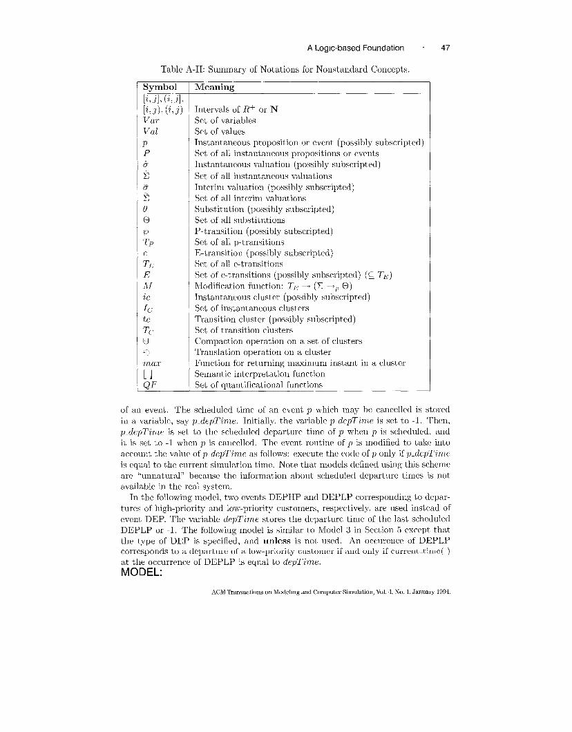
ALoglc-based Foundation “
Table A-II: Summary of Notations for Nonstandard Concepts.
Symbol
[i, j], (i, j],
[i,j), (i,j)
Var
Val
PP
6
2
8
E
0
G
@
TP
e
T~
E
M
ic
Ic
tc
TC
B
w
mu.z
[1QF
Meaning
Intervals of R+ or N
Set of variables
Set of values
Instantaneous proposition or event (possibly subscripted)
Set of all instantaneous propositions or events
Instantaneous valuation (possibly subscripted)
Set of all instantaneous valuations
Interim valuation (possibly subscripted)
Set of all interim valuations
Substitution (possibly subscripted)
Set of all substitutions
P-transition (possibly subscripted)
Set of all p-transitions
E-transition (possibly subscripted)
Set of all e-transitions
Set of e-transitions (possibly sl~bscripted) (~ TE)
Modification function: TE ~ (Z 4P ~)
Instantaneous cluster (possibly subscripted)
Set of instantaneous clusters
Transition cluster (possibly subscripted)
Set of transition clusters
Compaction operation on a set of clusters
Translation operation on a cluster
Function for returning maximum instant in a cluster
Semantic interpretation function
Set of quantificational functions
47
scheduled time of an event p which may be cancelled is storedof an event. The
in a variable, say p-depTime. Initially, the variable p-depTin~e is set to -1. Then,
p_depTime is set to the scheduled departure time of p when p is scheduled, and
it is set to -1 when p is cancelled. The event routine of p is modified to take into
account the value of p_depTime as follows: execute the code of p only if ~~_depTime
is equal to the cllrrent simulation t imc. Note that models defined using this scheme
are “unnatural” because the information about scheduled departlme times is not
available in the real system.
In the following model, two events DEPHP and DEPLP corresponding to depar-
tures of high-priority and low-priority customers, respectively, are l~sed instead of
event DEP. The variable depTime stores the departure time of the last scheduled
DEPLP or -1. The following model is similar to Model 3 in Section 5 except that
the type of DEP is specified, and unless is not used. An occurence of DEPLP
corresponds to a departure of a low-priority customer if and only if cument.time( )
at the occurrence of DEPLP is equal to depTime.
MODEL:
ACM Transactions on Modeling and Computer Skmdation, Vol. -L,No. 1, January 1994.

48 . A. Radiya and R. G. Sargent
Table B-I: Quantificational Flmctions
quantificational
function qf ~f(~> !4)
n ezf if 1 ~ Z- then {{l}} else @
If if O E y then {{O}} else {#}
whe~l if y # ~ then {{least(y)}} else {4}
Ljhener]er {Y}unless if y = @ then {{0}} else {@}
some ify#@then {ulu~2andy flu#~}else~
untd if y # @ then {[0, least(y))} else {z}
uhde {c-segment of y at 0}
at if y # 4 then {{least(y)}} else @
/* Initialization formula (same as lines 1-2 in NIodcl 3). */
1. {status := free; ql.high := O; ql.lvw := O; depTime := -1;
2. if (type( ) = htgh) then {after interarrival( ) HPCA}
else {after int erarrival( ) LPCA} }
/* Either type of customer arrives (same as lines 3-4 in Model 3). */
3. {whenever (HPCA or LPCA)
4. if (type( ) = high) then {after intm-arrival( ) HPCA}
else {after interarrival( ] LPCA}}
/’ The following formula modifies lines 7 and 8 in Model 3. “/
5. {whenever (HPCA) /* A high-priority customer arrives */
6. {{ StdLLS := bWS’@Li(J/i }
7. II {if (wDEPHP & status = busy-high)
then ql-h:lgh := ql.high + 1 else {after service( ) DEPHP}}
8. II {if ((wDEPLP or (DEPLP & current_time( ) # depl’ln~e)) &
status = busg-low]
then {{ql.low := ql.loti + 1} II {depTime := -l}}}}}
/* Insert a preempted customer in the low-priority cutorners queue and set
depTzrne to -1.A f’akc occurrence of DEPLP is specified by (DEPLP &
curren.tirne( ) # depTin~e). */
/“ The following formula is the same as formula of Model 3 at lines 9-14 except
the type of DEP is specified and unless is rcmovc(l. */
9. {whenever (LPCA) /* A low-priority customer arrives */
10. if (status = free or (( DEPHP or (DEPLP & current.time( ) = depTime))
& ql-high = O))
11. then {{status := bus~.low}
II {temp := service( ); depTzme := current.time( ) + ten~p;
{after ternp DEPLP}}}
12. else {{ql_loul := ql_low + 1}
13. II {if (DEPHP) then {{ql-high := ql.high - 1}
14. [1 {status:= busy-high} II {after service( ) DEPHP}}}}}
ACM Transactmns on Modeling and Computer Simulation, Vol. 4, No 1, January 1994
ALogic-based Foundation e 49
/“ The following formula is the same as lines 15-20 in Model 3 except the type
of DEP is specified and unless is removed. */
15. {whenever (DEPHP & N(HPCA or LPCA) ) /* Only departure of a
high-priority occurs */
16. if (ql.high > O) then {ql.h,igh := ql-high – 1;{after servicc( ) DEPHP}}
17. else if (ql-loul > O)
18. then {{ql-low := ql.lou – 1} II {status := busy_tow}
19. II {temp := service( ); depTime := current_time( ) + temp;
{after ternp DEPLP}}}
20. else status := free}
/* DEPLP corresponds to only a departure of a low-priority customer if
depl’zm,e = current _time( ). The following formula is similar to lines 15 and
17-19in Model 3 except the type of DEP is specified and unless is removed. */
21. {whenever (DEPLP & N(HPCA or LPCA))
22. if (depTtme = current_time( ))
23. then if (qi-low > O)
24. then {{ql-low := ql_low – 1}
II{ternp := service( ); depTime := current_time( ) + temp;
{after ternp DEPLP}}}
25. else status := free}
ACKNOWLEDGMENTS
The authors thank the anonymous referees for useful suggestions which have sig-
nificant ly improved the presentation of this article. The first author would like to
thank Vibha Radiya for careful reading of the article and help with the figures and
tables.
REFERENCES
ALLEN, J. F. 1984. Towards a general theory of action and time. Art. Intell. 23,
2 (Feb.), 123–154.
BARWISE, J. 1985. Model-theoretic logics: Background and aims. In Model-
Theoretic Logics. Springer-Verlag, New York, 3-23.
BARWISE, J. AND COOPER, R. 1981. Generalized quantifiers and natural lan-
guage. Lmg. Philos. 4, 159-219.
BROWN, M. 1984. Generalized quantifiers and the square of opposition. Notre
Dame J. of Formal Logw 25, 4 (Ott.), 303-322.
COTA, B. A. AND SARGENT, R. G. 1992. A modification of the process inter-
action world view. ACM Trans. Model. Comput. Simul. 2, 2 (Apr.), 109–129.
DOWTY, D. R., WALL, R. E., AND PETERS, S. 1981. Introduction to Montague
Semanttcs. D. Rcidel, Dordrecgt, Holland.
FUTO, 1. AND GER~ELY, T. 1982. A logical approach to simulation. In Adequate
Modehng of Systems. Springer-Verlag, New York, 25-46.
GIUNCHIGLIA, F. AND WALSH, T. 1990. A theory of abstraction. Res. Paper
ACM TransactIons on Modeling and Computer Simulation, Vol. 4, No. 1, January 1994
50 “ A. Radiya and R. G. Sargent
516, Dcpt. of Artificial Intelligence, IJniv. of Edinburgh. To appear in J.
Artif. Intell.
GLYNN, P. W. 1989. A GShlP formalism for discrete event systems. Proc. IEEE
77, 1 (Jan.), 14–23.
HOARE, C. A. R. 1985. Communtcattng $equentzal Processes. Prentice-Hall In-
ternational, Englewoods Cliffs, N..J.
Hoo\’EIt, J. W. AND REILLY) K. D. 1982. An algorithmic analysis of simulation
strategies. Int. J. Comput. Inf. Scz. 11, 2, 101-121.
HOROWITZ, E. 1984. Fundamentals of Programmmg Languages. 2nd eel. Com-
puter Science Press, Rockville, NM.
KA.hIP, H. W. 1!368. Tense logic and the theory of linear order. Ph.D. dissertation.
Univ. of California, Los Angeles.
KIVIAT, P. J. 1971. Simulation langllages. In Computer Simulation Experiments
with Models of Eco~wmic Systems. Wiley, New York, 406–489.
KOWALSKI, R. AND SERGOT, N/I. 1986. A logic-based calculus of events. New
Gen. Comput. 4, 67-95.
KRIPKE, S. 1963. Semantic considerations on modal logic. Acts PMos. Fenn.
16, 83-94.
KROGER, F. 1987. Temporal Logic o,f Progrums. EATCS Monograph OIL Theo-
retical Computer Science. Springer-Vcrlag, New York.
NANCE. R. E. 1981. The time and state representation in simulation modeling.
Commun. ACM 24, 4 (Apr.), 173-179.
NARAIN, S. 1991. An axiomatic basis for geueral discrete event modeling. In
Proceedin,qs of the 1991 Winter Simulation Con~erence. IEEE, New York,
1073-1082.
OSTRO~F, J. S. 1989. Temporal Logic for ,~eal-tzme Systems. Wiley, New York.
OVERSTREET, C. NT. AND NANCE. R. E. 1!185. A specification language to assist
in analysis of discrete event simldation models. ComnLun. ACM 28, 2 (Feb.),
190-201.
RADIYA, A. 1990. A logical approach to discrete event modeling and simulation.
Ph.D. dissertation. School of Computer and Information Science, Syracuse
Univ., Syracuse, N.Y.
RADIYA, A. AND SARGENT, R. G. 1987. Logic programming and discrete event
simulation. In S’tm,ulation and Al Simulation Series, vol. 18, no. 3, Society
for Computer Simulation, San Diego, Calif., 64--71.
RAiVIADGE, P. J. G. AND WONH.AIM, W. N1. 1989. The control of discrete event
systems. Proc. IEEE 77, 1 (Jan.), 81–98.
ROBINSON, .J. A. 1979. Logic: Form and Function. North-Holland, Amsterdam.
SHOHAM, Y. 1987, Temporal logics in AI: ;Semantical and ontological consider-
ations. Art. Intell. 33, 89–104.
TOURETZKY, D. S. 1986. The Muthernatics of Inheritance Systems. Morgan
Kaufmann, San NIateo, C~alif.
WOLPER, P. 1983. Temporal logic can be more expressive. fn~. Control 56, 72-79.
ZEIGLER, B. P. 1976. Theory of Modelling and Simulation. Wiley, New Korli.
ACM Transactions on Modeling and Computer Simulation, Vol 4, No. 1, January 1994.
ALoglc-based Foundation “ 51
ZEIGLER, B. P. 1984. Multifaceted Modelling and Discrete Event Simulation.
Academic Press, New York.
ZEIGLER, B. P. 1990. Object Ortented Swnulation wtth Hwrarchtcal Modular
Models. Academic Press, New York.
Received Julv 1992; rewsed March 1993; accepted N’Iay 1993
ACM Transactions on Modeling amd Computer Smmlation, Vol. 4, No. 1, January 1994.