A guide to using OLI Flowsheet: ESP Guides/OLI Flowsheet 9... · A guide to using OLI Flowsheet:...
195
A guide to using OLI Flowsheet: ESP 1 Getting Started with OLI Flowsheet A guide to using OLI Flowsheet: ESP Version 9.6 OLI Systems, Inc.
Transcript of A guide to using OLI Flowsheet: ESP Guides/OLI Flowsheet 9... · A guide to using OLI Flowsheet:...
A guide to using OLI Flowsheet: ESP 1 Getting Started with OLI Flowsheet
A guide to using OLI Flowsheet: ESP Version 9.6 OLI Systems, Inc.
A guide to using OLI Flowsheet: ESP 2 Getting Started with OLI Flowsheet
Copyright© 2018 OLI Systems, Inc. All rights reserved.
The enclosed materials are provided to the lessees, selected individuals and agents of OLI Systems, Inc. The material may not be duplicated or otherwise provided to any entity without the expressed permission of OLI Systems, Inc.
240 Cedar Knolls Road Suite 301
Cedar Knolls, NJ 07927 973-539-4996
(Fax) 973-539-5922 [email protected]
www.olisystems.com
Disclaimer: This manual was produced using the OLI Flowsheet: ESP - version 9.6.1 using the 9.6.1 databases. As time progresses, new data and refinements to existing data sets can result in values that you obtain being slightly different than what is presented in this manual. This is a natural progress and cannot be avoided. When large systematic changes to the software occur, this manual will be updated.
A guide to using OLI Flowsheet: ESP 3 Getting Started with OLI Flowsheet
Table of Contents Chapter 1. Getting Started with OLI Flowsheet ............................................................................................. 7
A tour of OLI Flowsheet: ESP – The basics ......................................................................................................... 7
Creating the Process ..................................................................................................................................... 7
Starting the tour............................................................................................................................................ 8
Defining the chemistry for this application ................................................................................................. 11
Building the process .................................................................................................................................... 15
Running the calculation .............................................................................................................................. 22
Obtaining preliminary results ...................................................................................................................... 23
Finishing the application ............................................................................................................................. 25
Running the final simulation design ............................................................................................................ 31
A tour of OLI Flowsheet: ESP – Some Advanced Features ............................................................................... 33
A tour of OLI Flowsheet: ESP – More Advanced Options ................................................................................ 43
Modifying the chemistry ............................................................................................................................. 43
Chapter 2. Process Options .......................................................................................................................... 53
Overview ......................................................................................................................................................... 53
Menu Items ..................................................................................................................................................... 53
Toolbar ............................................................................................................................................................ 57
Adding callouts............................................................................................................................................ 58
Editing a callout .......................................................................................................................................... 59
Editing the units for a callout ...................................................................................................................... 62
Copy and Paste a callout ............................................................................................................................. 65
Process Options .............................................................................................................................................. 67
Optional Properties ..................................................................................................................................... 67
Recycles ...................................................................................................................................................... 67
Restart Options ........................................................................................................................................... 70
Molecular Conversion Weights ................................................................................................................... 70
Liq-2 Key Component .................................................................................................................................. 71
Calculation Aids ........................................................................................................................................... 71
Block Calculation Order............................................................................................................................... 71
Chapter 3. Reports ....................................................................................................................................... 73
Stream Report ................................................................................................................................................. 73
Block Report .................................................................................................................................................... 75
Multi-stream Report ....................................................................................................................................... 75

A guide to using OLI Flowsheet: ESP 4 Getting Started with OLI Flowsheet
Overall Process Balance Report ...................................................................................................................... 76
Chapter 4. Chemistry Models ...................................................................................................................... 77
Overview ......................................................................................................................................................... 77
Chemistry Tab ............................................................................................................................................. 77
Inflows Tab .................................................................................................................................................. 81
Phases Tab .................................................................................................................................................. 86
Redox Tab ................................................................................................................................................... 88
Kinetics Tab ................................................................................................................................................. 91
T/P Span ...................................................................................................................................................... 94
Chapter 5. Process Modeling ....................................................................................................................... 96
Overview ......................................................................................................................................................... 96
Unit Operations/Blocks and Controllers .......................................................................................................... 96
Unit Operations/Blocks and Controllers Summary Descriptions ..................................................................... 97
1. Mixer .................................................................................................................................................. 97
2. Separator ............................................................................................................................................ 97
3. Neutralizer .......................................................................................................................................... 97
4. Splitter ................................................................................................................................................ 98
5. Component Splitter ............................................................................................................................ 98
6. Absorber ............................................................................................................................................. 98
7. Stripper/Distillation Column ............................................................................................................... 99
8. Extractor Unit ..................................................................................................................................... 99
9. Reactor ............................................................................................................................................. 100
10. Filter ............................................................................................................................................. 100
11. Settler ........................................................................................................................................... 100
12. Compressor .................................................................................................................................. 101
13. Turbine ......................................................................................................................................... 101
14. Heat Exchanger ............................................................................................................................ 101
15. Incinerator .................................................................................................................................... 102
16. Feedback Controller ..................................................................................................................... 102
17. Feed-forward Controller ............................................................................................................... 102
18. Manipulator .................................................................................................................................. 102
19. Pump ............................................................................................................................................ 103
20. RO Membranes (Reverse Osmosis) .............................................................................................. 103
Details of Unit Operations/Blocks ................................................................................................................. 104
A guide to using OLI Flowsheet: ESP 5 Getting Started with OLI Flowsheet
1. Mixer Unit ......................................................................................................................................... 104
2. Separator Unit .................................................................................................................................. 105
3. Neutralizer Unit ................................................................................................................................ 106
4. Splitter Unit ...................................................................................................................................... 108
5. Absorber Unit ................................................................................................................................... 110
6. Distillation/Stripper Unit ................................................................................................................... 114
7. Extractor Unit ................................................................................................................................... 120
8. Reactor Unit ..................................................................................................................................... 122
9. Filter Unit .......................................................................................................................................... 126
10. Settler Unit ................................................................................................................................... 127
11. Compressor Unit .......................................................................................................................... 129
12. Turbine Unit ................................................................................................................................. 131
13. Heat Exchanger Unit ..................................................................................................................... 132
14. Incinerator .................................................................................................................................... 134
15. Feedback Controller ..................................................................................................................... 135
16. Feedforward Controller Unit ........................................................................................................ 138
17. Manipulator Unit .......................................................................................................................... 140
18. Pump ............................................................................................................................................ 141
19. RO Membranes (Reverse Osmosis) .............................................................................................. 142
Chapter 6. Process Applications ..................................................................................................................... 148
6.1. Reactor Block .................................................................................................................................... 148
6.1.1. Standard Reaction Kinetics ....................................................................................................... 148
6.1.2. Non-Standard (User Defined) Reaction Kinetics ....................................................................... 155
6.1.3. Stoichiometric Reactors (CONV) ............................................................................................... 161
6.1.4. Gibbs Reactor ........................................................................................................................... 165
6.2. Sensitivity Analysis ............................................................................................................................ 169
HF Titration ............................................................................................................................................... 169
Chemistry and Thermodynamic Framework ............................................................................................. 169
Flowsheet.................................................................................................................................................. 169
Composition and setup ............................................................................................................................. 170
Create Analysis .......................................................................................................................................... 171
Monitored Variables ................................................................................................................................. 172
Add Sensitivity Plot ................................................................................................................................... 174
6.3. RO Membranes (Reverse Osmosis) .................................................................................................. 177

A guide to using OLI Flowsheet: ESP 6 Getting Started with OLI Flowsheet
Overview of RO ......................................................................................................................................... 177
Defining the Chemistry Model .................................................................................................................. 177
Defining the Flowsheet ............................................................................................................................. 178
Entering the stream and block parameters (except the RO membrane). ................................................. 178
Defining the RO Membrane Block ............................................................................................................. 182
Running the simulation ............................................................................................................................. 186
Chapter 7. Appendix .................................................................................................................................. 188
OLI MEMBRANE TECHNOLOGY: SIMULATOR FOR REVERSE OSMOSIS PROCESS .......................................... 188
Summary ................................................................................................................................................... 188
Model Development ................................................................................................................................. 189
Permeability Estimate ............................................................................................................................... 190
References ................................................................................................................................................ 191
Definitions ..................................................................................................................................................... 192
Manufacturer Data Sheet for RO Membranes .............................................................................................. 194
A guide to using OLI Flowsheet: ESP 7 Getting Started with OLI Flowsheet
Chapter 1. Getting Started with OLI Flowsheet
A tour of OLI Flowsheet: ESP – The basics This tour of OLI Flowsheet: ESP is based on a sample application - a pH neutralization problem. Suppose we have two waste streams that must be mixed together. One of the streams is an acid stream (in that the pH is less than 7.0 at room temperature) and the other stream is a base stream. We know from general chemistry that when acid and base streams mix, generally heat is evolved resulting in gases being produced. In addition, if the pH changes significantly, solids may form.
We want to treat any resulting gases from this mixing separately (we may need to recover the gases for another process) and we also want to remove any solids which may form. Finally, we want to make sure that the pH of the resulting liquid has been made basic.
Creating the Process
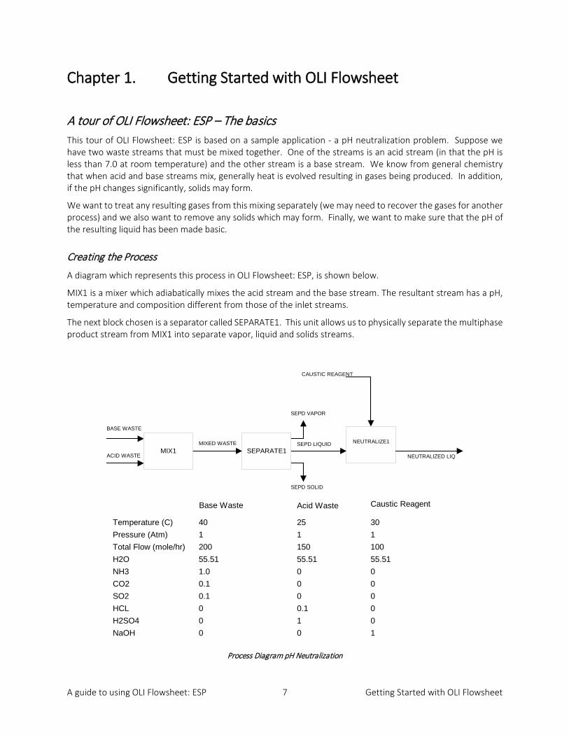
A diagram which represents this process in OLI Flowsheet: ESP, is shown below.
MIX1 is a mixer which adiabatically mixes the acid stream and the base stream. The resultant stream has a pH, temperature and composition different from those of the inlet streams.
The next block chosen is a separator called SEPARATE1. This unit allows us to physically separate the multiphase product stream from MIX1 into separate vapor, liquid and solids streams.
Process Diagram pH Neutralization
MIX1 SEPARATE1NEUTRALIZE1
BASE WASTE
ACID WASTE
MIXED WASTE SEPD LIQUID
SEPD VAPOR
SEPD SOLID
NEUTRALIZED LIQ
CAUSTIC REAGENT
Base Waste Acid Waste Caustic Reagent
Temperature (C) 40 25 30Pressure (Atm) 1 1 1Total Flow (mole/hr) 200 150 100H2O 55.51 55.51 55.51NH3 1.0 0 0CO2 0.1 0 0SO2 0.1 0 0HCL 0 0.1 0H2SO4 0 1 0NaOH 0 0 1
A guide to using OLI Flowsheet: ESP 8 Getting Started with OLI Flowsheet
The combination of the mixer and separator represents a surge tank. Generally, a surge tank would be used in a pH neutralization process to dampen flow and composition fluctuations as well as to vent vapor release and to settle solids.
The neutralizer block then adds a reagent to adjust the pH of the liquid from that of the separator effluent liquid to the desired value.
The following instructions are designed to take you on a tour through some of the interesting features of the OLI Flowsheet: ESP Process Analysis facilities.
Starting the tour
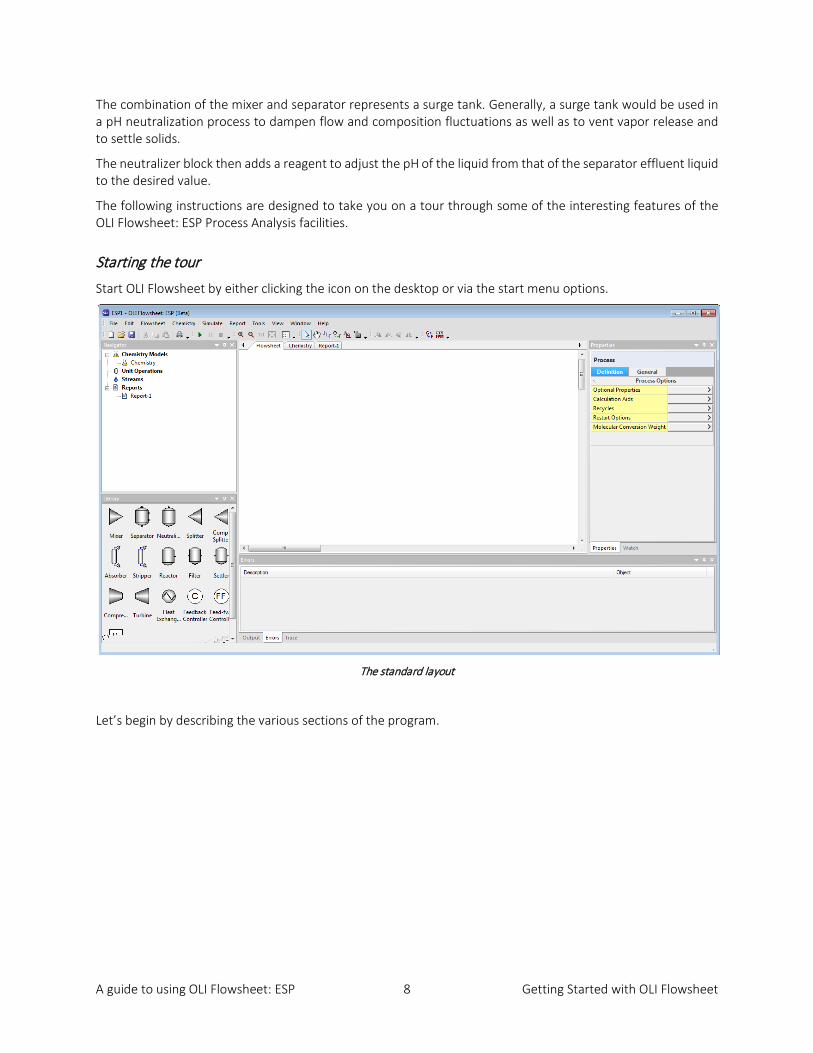
Start OLI Flowsheet by either clicking the icon on the desktop or via the start menu options.
The standard layout
Let’s begin by describing the various sections of the program.
A guide to using OLI Flowsheet: ESP 9 Getting Started with OLI Flowsheet
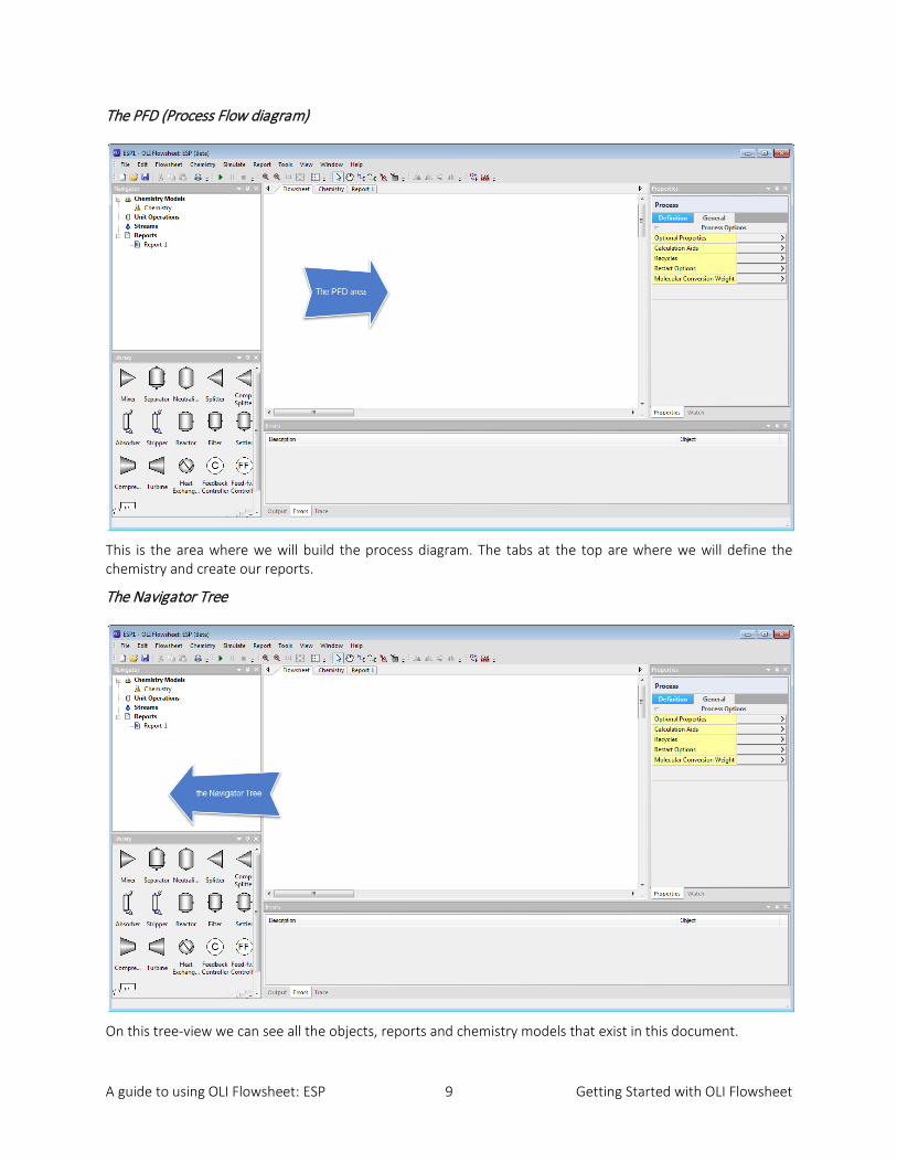
The PFD (Process Flow diagram)
This is the area where we will build the process diagram. The tabs at the top are where we will define the chemistry and create our reports.
The Navigator Tree
On this tree-view we can see all the objects, reports and chemistry models that exist in this document.

A guide to using OLI Flowsheet: ESP 10 Getting Started with OLI Flowsheet
Unit Operations
This is the palate of unit operations available in OLI Flowsheet: ESP. These will be described in more detail in the following chapters.
Properties
This window changes depending on the object highlighted. Right now, it is displaying options for the entire flowsheet.
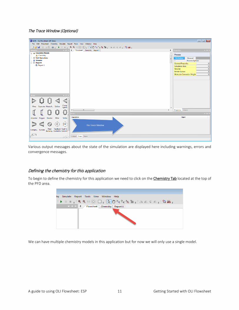
A guide to using OLI Flowsheet: ESP 11 Getting Started with OLI Flowsheet
The Trace Window (Optional)
Various output messages about the state of the simulation are displayed here including warnings, errors and convergence messages.
Defining the chemistry for this application
To begin to define the chemistry for this application we need to click on the Chemistry Tab located at the top of the PFD area.
We can have multiple chemistry models in this application but for now we will only use a single model.

A guide to using OLI Flowsheet: ESP 12 Getting Started with OLI Flowsheet
If you have used other OLI Software before then many of the objects on this screen will be familiar to you. We will describe them here.
The default view of the chemistry tab is the Databanks Tab. Here we have several buttons and fields.
Thermodynamic Framework Button
Here we can choose which thermodynamic framework for the simulation. For this application use the default framework of Aqueous (H+ Ion).
Adding user/private databanks
The user can add some additional databanks or their own databanks. This is usually required when the default OLI databank is either too broad in converge or was missing some components. The currently selected databanks are displayed (Public in this example) but addition databanks can be selected via the Add button.

A guide to using OLI Flowsheet: ESP 13 Getting Started with OLI Flowsheet
These databanks will be discussed in later chapters. For this application do not select any additional databanks.
Creating the inflow chemistry
Now click on the Inflows Tab to enter the inflow list of components.
Entering components.
We can start to enter the name of our components. Experienced uses of OLI software know that they can either type in the chemical formula or enter the OLI TAG name. The inflow grid will automatically start to search for your components. We can also add special components such petroleum assays and pseudo components via the Add button. This functionality will be discussed in later chapters.
For now, please enter the species name for ammonia, NH3
A guide to using OLI Flowsheet: ESP 14 Getting Started with OLI Flowsheet
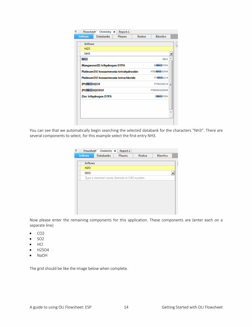
You can see that we automatically begin searching the selected databank for the characters “NH3”. There are several components to select, for this example select the first entry NH3.
Now please enter the remaining components for this application. These components are (enter each on a separate line)
• CO2 • SO2 • HCl • H2SO4 • NaOH
The grid should be like the image below when complete.
A guide to using OLI Flowsheet: ESP 15 Getting Started with OLI Flowsheet
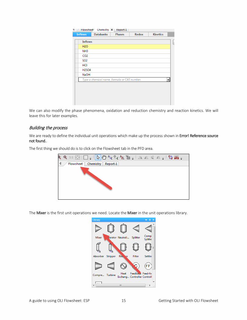
We can also modify the phase phenomena, oxidation and reduction chemistry and reaction kinetics. We will leave this for later examples.
Building the process
We are ready to define the individual unit operations which make up the process shown in Error! Reference source not found..
The first thing we should do is to click on the Flowsheet tab in the PFD area.
The Mixer is the first unit operations we need. Locate the Mixer in the unit operations library.

A guide to using OLI Flowsheet: ESP 16 Getting Started with OLI Flowsheet
Double-clicking the object will add it to the PFD.
A lot of messages and properties suddenly became visible in the program. The object is centered on the PFD by you can click and drag it where you want. Right now, it is acceptable where it is located. The Properties window has updated with some information. We will come back to this window. Right now, we need to add some streams. The mixer needs two inlets (although a single inlet is permitted) and a single outlet. To start adding streams we need to click the streams icon above the PFD in the tool bar.
The Streams toolbar button
Now position the mouse pointer near the inlet side of the mixer.

A guide to using OLI Flowsheet: ESP 17 Getting Started with OLI Flowsheet
As you click and drag the inlet select streams become visible as red lines. Just drop the end of the stream on the red line. Pressing the ESC key exits the add stream function if you so desire.
Added stream with the properties window displayed.
At this point you have some options. The desired stream name is “Base Waste” and you can change it now or later. Some users prefer to change the name as they go and others after the blocks are connected.
For this example, we will complete adding the inlet and outlet stream.
Re-click the Add Stream toolbar button and add a second inlet stream and then an outlet stream. You diagram should look like the following figure.

A guide to using OLI Flowsheet: ESP 18 Getting Started with OLI Flowsheet
Now let’s change the stream names to match Error! Reference source not found.. Like any good windows-based program there are several methods to accomplish this task. The first is to double-click the stream to put you into edit mode. Double-click the stream S-1 (or whatever name currently exists).
The name of the stream is highlighted. You can now just type the name you desire. In this case please change the name to “Base Waste”.
The text can be moved around to make the PFD more readable. We will do that in a later chapter.
The other method to change the name of a stream is to use the property window. In this case just click the stream “S-2”
Changing the stream name via the properties window
Click the General tab in the properties window for this stream.
A guide to using OLI Flowsheet: ESP 19 Getting Started with OLI Flowsheet
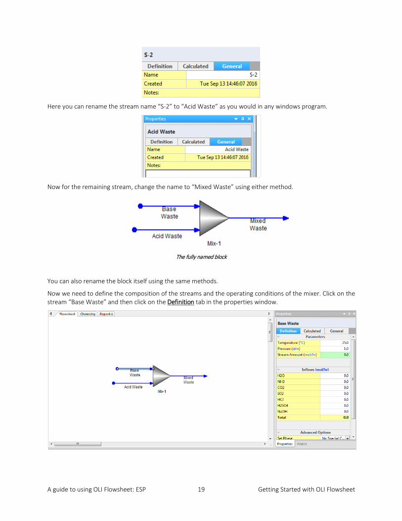
Here you can rename the stream name “S-2” to “Acid Waste” as you would in any windows program.
Now for the remaining stream, change the name to “Mixed Waste” using either method.
The fully named block
You can also rename the block itself using the same methods.
Now we need to define the composition of the streams and the operating conditions of the mixer. Click on the stream “Base Waste” and then click on the Definition tab in the properties window.

A guide to using OLI Flowsheet: ESP 20 Getting Started with OLI Flowsheet
The composition of Base-Waste is given in the Table below:
Stream Name Base Waste
Temperature, oC 40.0
Pressure, Atm 1.0
Stream Amount, mole/hr 200
Inflows, mol/hr
H2O 55.51
NH3 1.0
CO2 0.1
SO2 0.1
Enter these values in the grid; notice that we have not entered any values for HCl, H2SO4 or NaOH.

A guide to using OLI Flowsheet: ESP 21 Getting Started with OLI Flowsheet
A few comments about this stream; notice that the “Stream Amount” and the “Total” do not match. This is by design. Many times, a user will know the stream amount in a different unit such as kg/hour and the inflows in mass fractions. In that scenario, the two values do not match. What the internal numerical engine will do is to normalize the inflows to match the stream amount.
Please enter the composition for the stream “Acid Waste” in the same manner.
Stream Name Acid Waste
Temperature, oC 25.0
Pressure, Atm 1.0
Stream Amount, mole/hr 150
Inflows, mol/hr
H2O 55.51
HCl 0.1
H2SO4 1.0
Now we are ready to define the unit operation parameters.
Click on the mixer block.
In the properties window, we have several options. These options differ for each type of unit operation. We can see the names of the inlet streams and outlet streams. We can use the drop-down arrows to select different streams if required.
Please look at the section labeled “Equilibrium Calculation.” Here we can set some basic parameters for a mixer block.

A guide to using OLI Flowsheet: ESP 22 Getting Started with OLI Flowsheet
Calculation Type
We can have several types of calculations for a mixer. These will be described in detail in a later chapter. The default mixer type is “Adiabatic” which means the heat out of the block equals the sum of the heat into the block (duty = 0) and the temperature is calculated to meet that condition.
For this example, we will leave the Calculation Type at the default value of “Adiabatic”.
Pressure Spec.
Many unit operations have pressure options and these often depend on the type of calculation being specified. For our example, we will leave the default value of “Min. Inlet Pressure” which means we will survey the inlet streams and use the smallest value. In this example the inlet streams both have a pressure of 1.0 atmosphere so that will be the pressure used.
Heat Duty
For adiabatic type calculations (where the temperature is calculated) we can add some type of offset value. This is a rare calculation, so we will use the default value of 0.0.
Running the calculation
We have partially completed the process. There are several schools of thought on how to build a process. Some want to layout the process first then run the simulation. Others will build the process in parts and run each part. Both have advantages and disadvantages.
For this simulation, we will run the simulation for our partially completed process.
A guide to using OLI Flowsheet: ESP 23 Getting Started with OLI Flowsheet
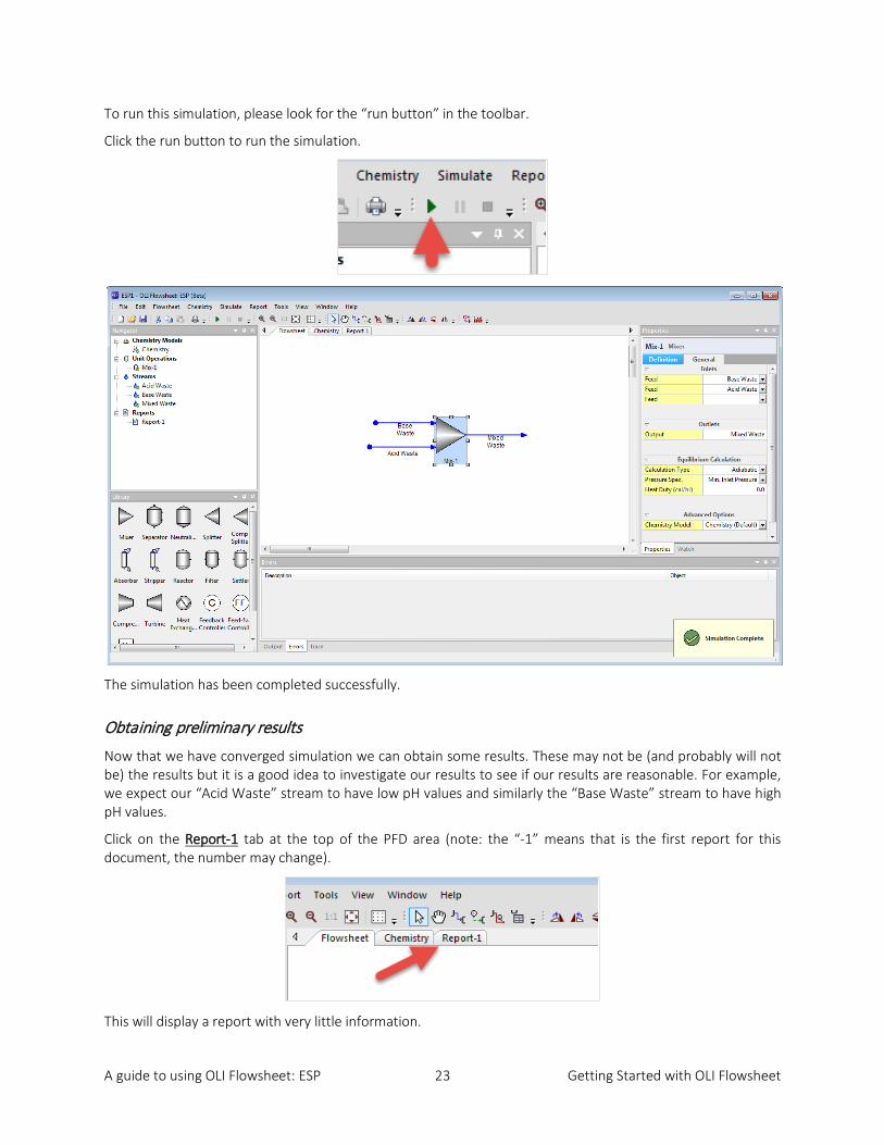
To run this simulation, please look for the “run button” in the toolbar.
Click the run button to run the simulation.
The simulation has been completed successfully.
Obtaining preliminary results
Now that we have converged simulation we can obtain some results. These may not be (and probably will not be) the results but it is a good idea to investigate our results to see if our results are reasonable. For example, we expect our “Acid Waste” stream to have low pH values and similarly the “Base Waste” stream to have high pH values.
Click on the Report-1 tab at the top of the PFD area (note: the “-1” means that is the first report for this document, the number may change).
This will display a report with very little information.

A guide to using OLI Flowsheet: ESP 24 Getting Started with OLI Flowsheet
We have many options here. We can see a single stream or multiple streams or all the streams. The process, currently, only has three streams. Click the Add All Streams hyperlink.

A guide to using OLI Flowsheet: ESP 25 Getting Started with OLI Flowsheet
This report is a table. It can be copied and pasted into another program such as Microsoft Word or Excel. You can use the Export button to create a CSV file for direct import into Excel. Right now, we will not dwell on too much of the contents since we have more unit operations to add. You can see, however, that our “Base Waste” and “Acid Waste” streams have pH values representative of the type of stream that they are.
Finishing the application
We will now finish the application by adding the remaining Separator and Neutralizer.
Click back on the Flowsheet tab above the PFD. From the Library please double-click the Separator unit operation.
Adding a separator block
You can see that double-clicking the unit operation put it dead-center in the PFD. There is a slightly better method of adding a block which we will show you with the neutralizer. For the drag the separator to the right of the mixer. Notice that a warning has appears informing you that the process definition has changed. Click the Dismiss button.
Now this part is tricky, click the arrowhead at the end of the stream “Mixed Waste” and drag it towards the separator “Sep-1.”
As you get close to the separator the inlet stream become live.

A guide to using OLI Flowsheet: ESP 26 Getting Started with OLI Flowsheet
Connect the “Mixed Waste” stream to any inlet stream.
Notice now that the connected stream went from blue (which indicates an inlet or outlet stream) to a thin black line. Thin black lines represent internal streams. Blue lines with a dot on the end are inlet streams and blue line with just an arrowhead our outlet streams.
As we did with the mixer we now need to add the outlet streams using the stream toolbar. Connect a line at the top, sides and bottom.
You will notice that as you add streams to a separator block we display some tags.
Displaying stream tags
These tags tell you what kind of stream is expected for that outlet port. The top stream is expected to be vapor and the bottom is solids. The top-most side stream is a liquid (water rich) and the bottom-most side stream is an organic stream (hydrocarbon-rich). We will discuss separators in more detail in later chapters.
The completed separator unit block now looks like this:

A guide to using OLI Flowsheet: ESP 27 Getting Started with OLI Flowsheet
We have started re-using the original stream names. We need to rename these streams according to the process design for pH neutralization shown on page 7.
Separator Stream Definitions – Sep-1
Line Name
Vapor Sepd Vapor
Liquid Sepd Liq
Organic Sepd Org
Solid Sepd Solid
Using the methods outlined for the mixer, change the name as indicated in the above table.
The separator also has its own properties which need to be defined. The separator also supports all the mixer calculations plus some entrainment options. We will not change any of these properties. The block properties are (we will use this table format for future examples).
Block Properties – Sept-1
Block Type Separator
Block Name Sep-1
Equilibrium Calculation
Calculation Type Adiabatic (default)
Pressure Spec. Min. Inlet Pressure (default)
Duty 0.0 (default)
Entrainment (sub-menu) All values are default

A guide to using OLI Flowsheet: ESP 28 Getting Started with OLI Flowsheet
We will now add the final block which is a neutralizer block. Locate the neutralizer block from the Library (you may need to scroll down to locate it).
This time do not double-click the block. Click and then drag it to the PFD.
This is not a very convenient place to locate the block. Using the scroll bars move the entire PFD to the left (scrolling right):
Scrolling right (moving left)

A guide to using OLI Flowsheet: ESP 29 Getting Started with OLI Flowsheet
Now drag the neutralizer up a bit to be in line with the other blocks.
As with the separator, drag the stream “Sepd Liq” to the neutralizer and connect to an inlet. Then add a new inlet stream to the top of the neutralizer. Rename the new inlet stream to “Caustic Reagent” and create an outlet stream named “Neutralized Liq”.
The process should look like the one shown in the figure below:

A guide to using OLI Flowsheet: ESP 30 Getting Started with OLI Flowsheet
Now let’s finish adding the component inflows and block properties.
Stream Name Caustic Reagent
Temperature, oC 30.0
Pressure, Atm 1.0
Stream Amount, mole/hr 100
Inflows, mol/hr
H2O 55.51
NaOH 1.0
Now we will enter the block properties for the neutralizer. The Calculation Type option has changed and will require you to use the drop-down menu to find the correct setting:
Block Type Neutralizer
Block Name Neutrl-1
Equilibrium Calculation
Calculation Type Fix pH
Pressure Spec. Min. Inlet Pressure (default)
pH 9.0

A guide to using OLI Flowsheet: ESP 31 Getting Started with OLI Flowsheet
Running the final simulation design
We are now ready to run the simulation for the final design. However, good computing practices dictate that we should save the simulation before we run it.
Click the File | Save menu item or use the Save toolbar button. This function is the same as the standard windows conventions. Save the file in folder where you remember the location.
OLI recommends the name “Neutral1-basic design” as the file name. The file type is “ESP”.
Click the run button.
Once complete, please click on the Report-1 tab. The original list of streams will still be there and updated with new data if necessary. As we did previously, please click the Add all streams hyperlink.
We can modify the current report to display or hide streams and contents. If you are already familiar with OLI Studio or OLI Analyzer, then you know much about the report sections for each stream. We previously looked at the streams “Base Waste” and “Acid Waste”. These streams are fairly straightforward to analyze, and we will not look at them here.
Click the Remove hyperlink under those streams to remove them from the report. You should have a screen like the following (you may need to scroll left or right to see all the values depending on your screen resolution).
Notice that the “Moles, True (mol/hr)” line for the streams “Sepd Org” and “Sepd Solid” equals zero (0.0). This means that these streams have zero content. For this analysis we can remove these streams from the report by clicking the Remove link.
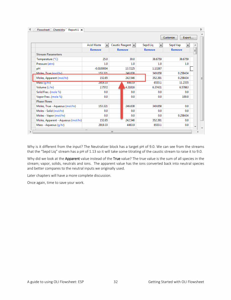
We now have a much more reasonable list. Going back to the flowsheet process presented on page 7 the original flowrate of the “Caustic Reagent” stream was 100 mol/hr. The value now is 242.5 mol/hr.
A guide to using OLI Flowsheet: ESP 32 Getting Started with OLI Flowsheet
Why is it different from the input? The Neutralizer block has a target pH of 9.0. We can see from the streams that the “Sepd Liq” stream has a pH of 1.13 so it will take some titrating of the caustic stream to raise it to 9.0.
Why did we look at the Apparent value instead of the True value? The true value is the sum of all species in the stream; vapor, solids, neutrals and ions. The apparent value has the ions converted back into neutral species and better compares to the neutral inputs we originally used.
Later chapters will have a more complete discussion.
Once again, time to save your work.

A guide to using OLI Flowsheet: ESP 33 Getting Started with OLI Flowsheet
A tour of OLI Flowsheet: ESP – Some Advanced Features In this application we will continue to use the example process Neutral1-basic design but will add a pH control loop rather than the neutralizer block. We frequently use a control loop for pH in cases where the set point of the controller is near the equivalence point of the solution (an area in which mathematical solutions are difficult to obtain).
We will be re-using portions of the NEUTRAL1 process1 described. The revised process diagram can be seen in the figure below.
Neutralization Process with Manipulate/Mix Block and pH Controller
Let’s save the file with a new name so we have the older file as a reference. Using the standard windows tools save the file with the name Neutral 1 – pH controller.
Locate the Neutrl-1 block on the existing PFD.
1Or use the name you supplied.
MIX1 SEPARATE1 NEUTRALIZE2MIX
CAUSTIC MANIPULATE
pH Control9.0
BASE WASTE
ACID WASTE
MIXED WASTE SEPD LIQUID
SEPD VAPOR
SEPD SOLID
NEUTRALIZED LIQ
CAUSTIC REAGENT
ADJUSTED CAUSTIC

A guide to using OLI Flowsheet: ESP 34 Getting Started with OLI Flowsheet
Press the delete key to remove this block.
Two things have happened at this point. First, the old neutralizer has been deleted but the associated inlet stream remains on the PFD. In addition, a warning has appeared to remind you that the process has been modified. To proceed, please click the Dismiss button at the top of the PFD.
We have several options now. You can either add the manipulator block as described above or start with a mixer. Either is acceptable. For this tour we will first add the new mixer and call it a neutralizer.
Select a Mixer from the library and drag it to approximately the same locate as the old neutralizer.
.
Change the parameters for the mixer as described in the following table:
Block Type Mixer
Block Name Neutrl-1
Inlet(s) Sepd Liq
Outlet(s) Neutralized Liq

A guide to using OLI Flowsheet: ESP 35 Getting Started with OLI Flowsheet
Equilibrium Calculation
Calculation Type Adiabatic
Pressure Spec. Min. Inlet Pressure
Heat duty 0.0
Advanced Options
Chemistry Model Chemistry (Default)
The PFD is now updated like this:
We now need to add a manipulator block. Manipulate blocks are very simple in operation. Either the total flow of the inlet stream is multiplied by some factor or a specific component in the stream is multiplied by a factor. This factor can be controlled by a Controller Block.
Locate the Manipulate block from the library and then drag it to the PFD above the Neutrl-1 block.
A guide to using OLI Flowsheet: ESP 36 Getting Started with OLI Flowsheet
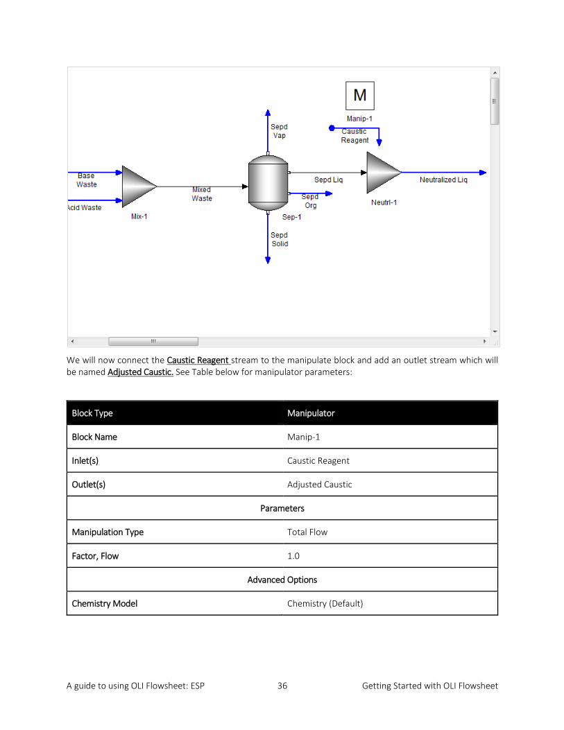
We will now connect the Caustic Reagent stream to the manipulate block and add an outlet stream which will be named Adjusted Caustic. See Table below for manipulator parameters:
Block Type Manipulator
Block Name Manip-1
Inlet(s) Caustic Reagent
Outlet(s) Adjusted Caustic
Parameters
Manipulation Type Total Flow
Factor, Flow 1.0
Advanced Options
Chemistry Model Chemistry (Default)

A guide to using OLI Flowsheet: ESP 37 Getting Started with OLI Flowsheet
The PFD should be updated as follows:
You may notice that we have moved blocks and streams around to make it easier to read the PFD. We will now add the final block for this process which is a control block. Locate the feedback controller from the library.
Now drag this block to slight above and to the right of the mixer “Neutrl-1”

A guide to using OLI Flowsheet: ESP 38 Getting Started with OLI Flowsheet
The connections to the controller are different than those of other blocks. The connections only carry information and not mass and energy. These connections are made with a different tool in the toolbar.
Controller connection tool
When you select this tool, you can drag lines from the measured object (usually a stream) to the controller and from the controller to the object under control (usually a block). Target points will appear when you drag the controller connector to the object.
Click the Controller Connector and drag a line from the stream Neutralized Liq to the Feedback-1 controller.
As the controller connection approaches, targets appear.
Select any one of them.
As the controller connect approaches the Feedback-1 block new targets appear
Complete the connections by dragging a line from the Feedback-1 controller to the Manip-1 block.

A guide to using OLI Flowsheet: ESP 39 Getting Started with OLI Flowsheet
The connected feedback controller
We now need to define the parameters for the feedback controller.
Block Type Feedback Controller
Block Name Feedback-1
Target Specification
Target Stream Neutralized Liq
Spec. Type pH
Target Value 9.0
Control Parameters
Controlling Block Manip-1
Block Parameter Factor, Flow
Options
Calculate After <Automatic>
Convergence Options Fly Out Menu (all default)
We are now ready to run the process. Like all good process simulators (that’s you!) please save the process first.

A guide to using OLI Flowsheet: ESP 40 Getting Started with OLI Flowsheet
Now run the process.
You may not see much going on. What we need to review is the following:
• pH of the Neutralized Liq stream • The flowrate of the Adjusted Caustic stream.
We can do this via the report feature we looked at previously, but we can get quick information directly on the PFD instead. We use a tool called “Callouts”.
Right-click the stream Neutralized Liq.
Select Add Callout.
Right-click to add Callout
A callout is displayed on the PFD (if it seems to have moved partially off screen you can grab it and drag it to where you can see it)
Callout for the stream "Neutralized Liq"
A guide to using OLI Flowsheet: ESP 41 Getting Started with OLI Flowsheet
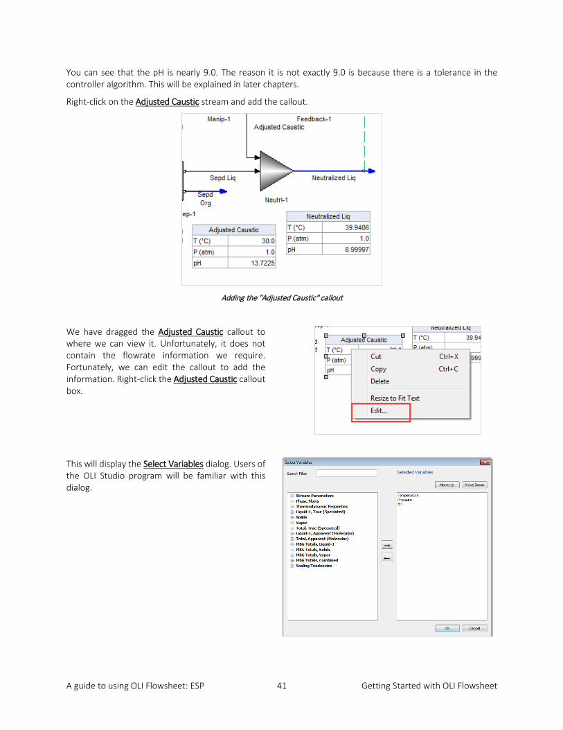
You can see that the pH is nearly 9.0. The reason it is not exactly 9.0 is because there is a tolerance in the controller algorithm. This will be explained in later chapters.
Right-click on the Adjusted Caustic stream and add the callout.
Adding the "Adjusted Caustic" callout
We have dragged the Adjusted Caustic callout to where we can view it. Unfortunately, it does not contain the flowrate information we require. Fortunately, we can edit the callout to add the information. Right-click the Adjusted Caustic callout box.
This will display the Select Variables dialog. Users of the OLI Studio program will be familiar with this dialog.
A guide to using OLI Flowsheet: ESP 42 Getting Started with OLI Flowsheet
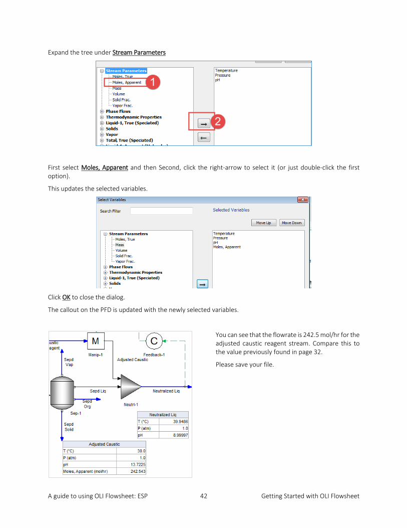
Expand the tree under Stream Parameters
First select Moles, Apparent and then Second, click the right-arrow to select it (or just double-click the first option).
This updates the selected variables.
Click OK to close the dialog.
The callout on the PFD is updated with the newly selected variables.
You can see that the flowrate is 242.5 mol/hr for the adjusted caustic reagent stream. Compare this to the value previously found in page 32.
Please save your file.

A guide to using OLI Flowsheet: ESP 43 Getting Started with OLI Flowsheet
A tour of OLI Flowsheet: ESP – More Advanced Options
We have just seen that a control block, combined with mix blocks and manipulate blocks, can be used to control the pH of a stream. Frequently a process recycles part or all of certain streams back to up-stream units. There are many reasons for this including minimization of waste, increase of residence time and purification of product.
This application extends the previous application by adding a new mix block, a split block and a recycle stream. We will be adding sodium chloride (salt) to the process to remove some solids from the solution. We will then recycle some of those solids back to an upstream unit to see the effect, if any, on the amount of caustic required to adjust the pH.
We will be reusing the previous process Neutral 1 – pH controller 2. Please load this file (if not already loaded) and then let’s save the file with a new name. OLI recommends Neutral 1 – recycle.
The figure below shows the layout of the new process.
Neutralization Process with Manipulate/Mix Block, pH Controller, and Recycle Loop.
Modifying the chemistry
For this example, we need to add some components to the chemistry model. Click the Chemistry tab at the top of the PFD.
2Or the name you supplied.
MIX1 SEPARATE1 NEUTRALIZE2MIX
CAUSTIC MANIPULATE
pH Control9.0
BASE WASTE
ACID WASTE
MIXED WASTE SEPD LIQUID
SEPD VAPOR
SEPD SOLID
NEUTRALIZED LIQ
CAUSTIC REAGENT
SalterMIX
Flow Splitter
Salt
PurgeStream
RECYCLE STREAM
SALTED STREAM
TEAR
ADJUSTED CAUSTIC

A guide to using OLI Flowsheet: ESP 44 Getting Started with OLI Flowsheet
Add the following components to the Inflows list:
• NaCl • NaHCO3 • Na2CO3 • Na2SO4 • (NH4)2SO4
Click Dismiss to clear the warning message and then click on the Flowsheet tab.
We are going to add a new mixer block and a new stream to the mixer. Please add these two objects to the PFD and connect them as indicated. The PFD should look like this (the details of the objects will follow):

A guide to using OLI Flowsheet: ESP 45 Getting Started with OLI Flowsheet
Stream Name Salt
Temperature, oC 25.0
Pressure, Atm 1.0
Stream Amount, mole/hr 75.0
Inflows, mol/hr
NaCl 75.0
Advanced Options
Set Phase Solids Only
Chemistry Model Chemistry(Default)
There is no water associated with this stream. Under most conditions, we require water as a component. In those cases, were we specifically do not want water in a stream, we must use the option.
In the table below, you will find the “Salter” Mixer parameters.
Block Type Mixer
Block Name Salter
Inlet(s) Neutralized Liq
Salt
Outlet(s) Salted Stream
Equilibrium Calculation
Calculation Type Isothermal
Pressure Spec. Min. Inlet Pressure
Temperature (oC) 40.0
Advanced Options
Chemistry Model Chemistry (Default)

A guide to using OLI Flowsheet: ESP 46 Getting Started with OLI Flowsheet
We will now split the Salted Stream to discharge some of the material and recycle some of the material. We now need to add a flow splitter to the PFD. A flow splitter is named “Splitter” in the library. By now you should be able to find unit operations in the library, so we will not show you an image for this.
Drag the Splitter and place it to the right of the Salted Stream on the PFD.
As with other objects we need to connect the streams. The Salted Stream will be connected to the inlet of the Split-1 block and two outlets will be defined, Purge and Recycle.
The parameters for the Split-1 block are found in the table below:
Block Splitter (flow)
Block Name Split-1
Inlets(s) Salted Stream
Outlet(s) Purge
Recycle
Parameters
Outlet Split Flyout (edit) This launches a new dialog (see Error! Reference source not found. Error! Reference source not found.
Advanced Options
Chemistry Model Chemistry (Default)

A guide to using OLI Flowsheet: ESP 47 Getting Started with OLI Flowsheet
Enter the fractions that you want to purge and recycle:
Click OK to close the dialog.
Right now, the PFD may look skewed or shifted to the right. We can zoon and center the diagram with a tool in the toolbar.
Click the Zoom to Fit tool button.
Zoom to Fit tool
We now need to connect the Recycle stream back to the upstream block Mix-1.

A guide to using OLI Flowsheet: ESP 48 Getting Started with OLI Flowsheet
The PFD should look that the image below:
This is a bit messy to read. We can drag our Recycle stream down to the PFD is easier to read. Click the stream and find one of the “Anchors” and drag the stream down.
Finding the "Anchor"
This PFD is certainly easier to read than the previous image.
A guide to using OLI Flowsheet: ESP 49 Getting Started with OLI Flowsheet
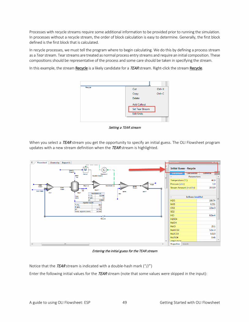
Processes with recycle streams require some additional information to be provided prior to running the simulation. In processes without a recycle stream, the order of block calculation is easy to determine. Generally, the first block defined is the first block that is calculated.
In recycle processes, we must tell the program where to begin calculating. We do this by defining a process stream as a Tear stream. Tear streams are treated as normal process entry streams and require an initial composition. These compositions should be representative of the process and some care should be taken in specifying the stream.
In this example, the stream Recycle is a likely candidate for a TEAR stream. Right-click the stream Recycle.
Setting a TEAR stream
When you select a TEAR stream you get the opportunity to specify an initial guess. The OLI Flowsheet program updates with a new stream definition when the TEAR stream is highlighted.
Entering the initial guess for the TEAR stream
Notice that the TEAR stream is indicated with a double-hash mark (“//”)
Enter the following initial values for the TEAR stream (note that some values were skipped in the input):

A guide to using OLI Flowsheet: ESP 50 Getting Started with OLI Flowsheet
TEAR Stream Initial Guess Recycle
Temperature, oC 40.0
Pressure, atm 1.0
Stream Amount, mole/hr 213.19
Inflows, mol/hr
H2O 186.74
NH3 0.331
CO2 0.002
HCl 0.0006
NaCl 25.1
NaHCO3 0.005
Na2CO3 0.023
Na2SO4 0.46
(NH4)2SO4 0.42
Process simulations with TEAR streams may take a long time to converge. We can monitor the approach to convergence with a tool called the Convergence Monitor. You enable the Convergence Monitor via the Menu > View >Windows and Toolbars > Convergence Monitor.
Enabling the convergence monitor
A guide to using OLI Flowsheet: ESP 51 Getting Started with OLI Flowsheet
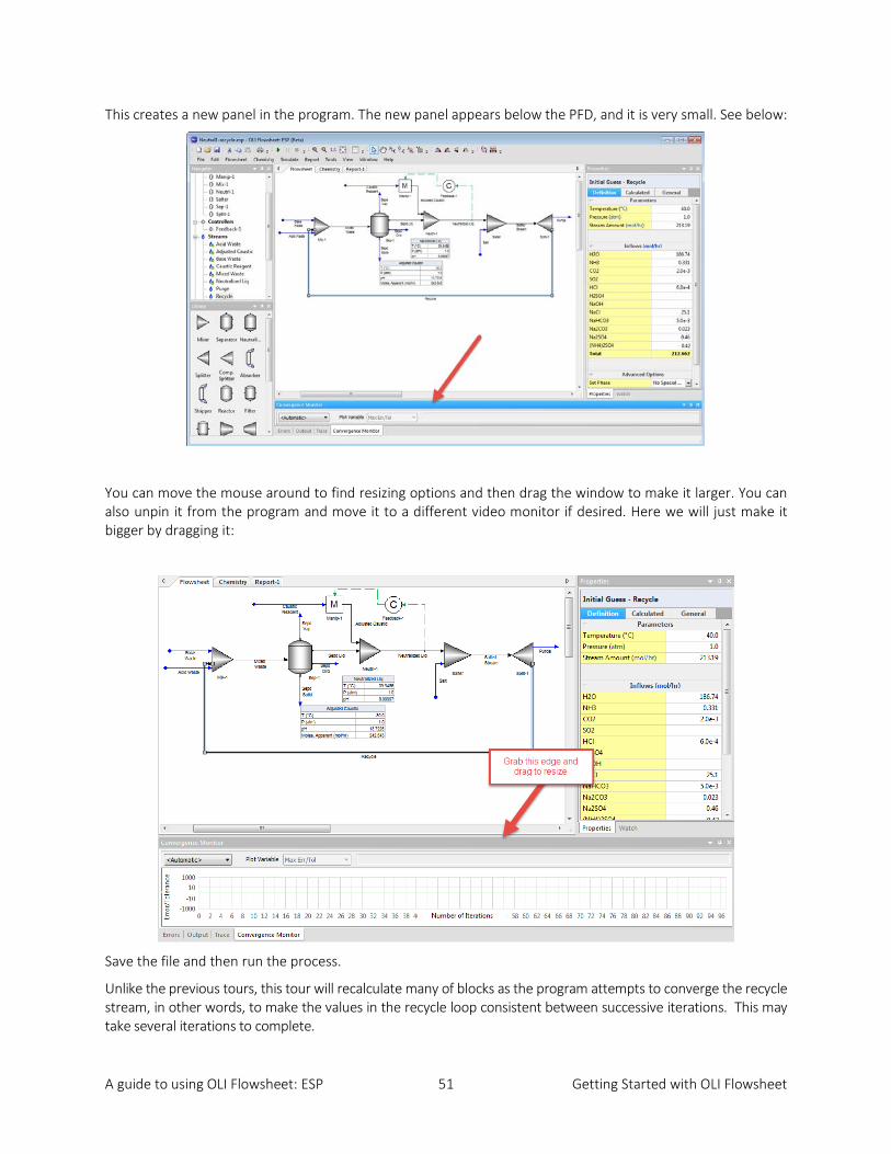
This creates a new panel in the program. The new panel appears below the PFD, and it is very small. See below:
You can move the mouse around to find resizing options and then drag the window to make it larger. You can also unpin it from the program and move it to a different video monitor if desired. Here we will just make it bigger by dragging it:
Save the file and then run the process.
Unlike the previous tours, this tour will recalculate many of blocks as the program attempts to converge the recycle stream, in other words, to make the values in the recycle loop consistent between successive iterations. This may take several iterations to complete.
A guide to using OLI Flowsheet: ESP 52 Getting Started with OLI Flowsheet
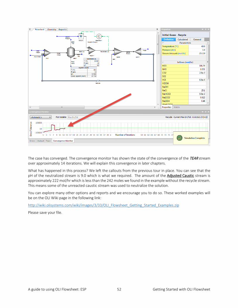
The case has converged. The convergence monitor has shown the state of the convergence of the TEAR stream over approximately 14 iterations. We will explain this convergence in later chapters.
What has happened in this process? We left the callouts from the previous tour in place. You can see that the pH of the neutralized stream is 9.0 which is what we required. The amount of the Adjusted Caustic stream is approximately 222 mol/hr which is less than the 242 moles we found in the example without the recycle stream. This means some of the unreacted caustic stream was used to neutralize the solution.
You can explore many other options and reports and we encourage you to do so. These worked examples will be on the OLI Wiki page in the following link:
http://wiki.olisystems.com/wiki/images/3/33/OLI_Flowsheet_Getting_Started_Examples.zip
Please save your file.

A guide to using OLI Flowsheet: ESP 53 Process Options
Chapter 2. Process Options
Overview The OLI Flowsheet screen is roughly divided into 6 sections. The top section (numbered 6) is Menu Items and Toolbar.
(1) Left most section is the Navigator Panel. The navigator panel will have the tree of all the objects in the current flowsheet.
(2) The middle section is Flowsheet window. This view can be switched by the tabs at the top to Chemistry view or Report view.
(3) The Properties Pane has two tabs, properties variables and watch variables. (4) The bottom section has four tabs, Errors, Trace, Convergence Monitor and Output. (5) Left bottom corner is the Library, it has all the unit operations.
Menu Items
Following image shows the menu items:
A guide to using OLI Flowsheet: ESP 54 Process Options
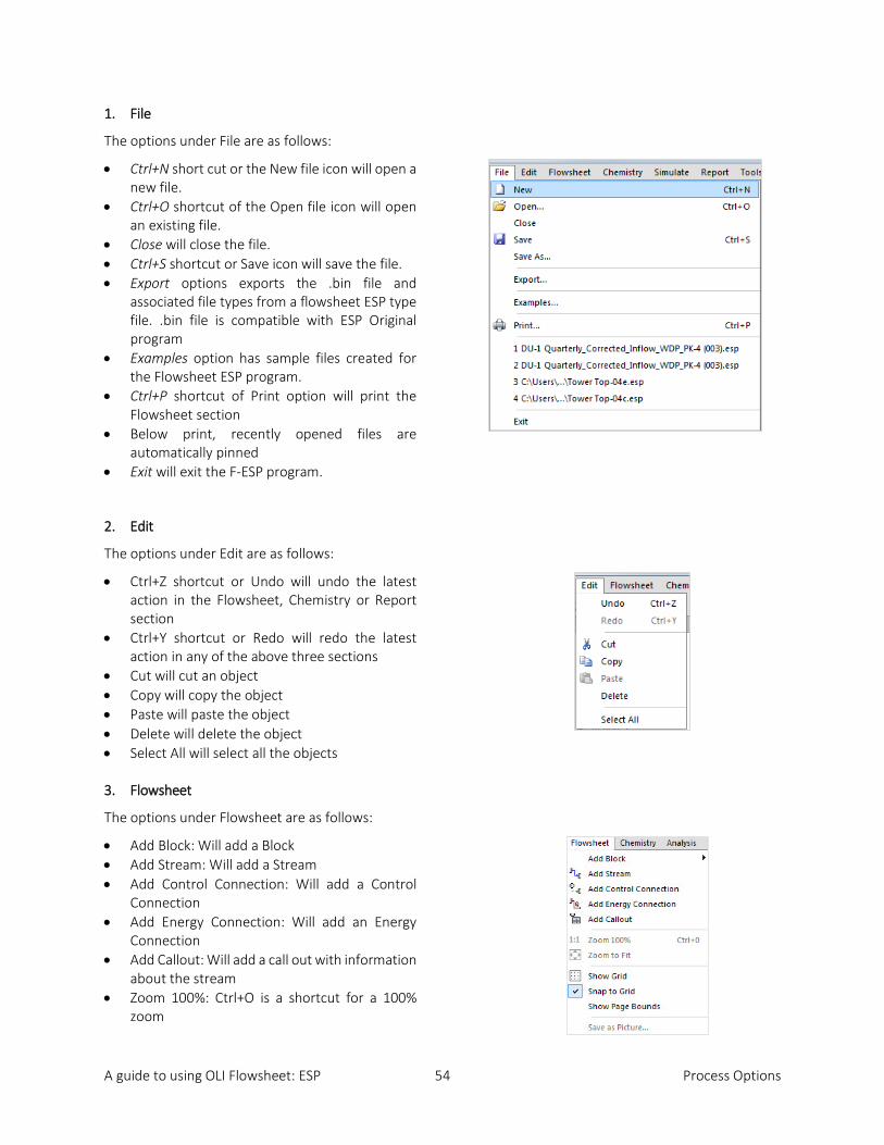
1. File
The options under File are as follows:
• Ctrl+N short cut or the New file icon will open a new file.
• Ctrl+O shortcut of the Open file icon will open an existing file.
• Close will close the file. • Ctrl+S shortcut or Save icon will save the file. • Export options exports the .bin file and
associated file types from a flowsheet ESP type file. .bin file is compatible with ESP Original program
• Examples option has sample files created for the Flowsheet ESP program.
• Ctrl+P shortcut of Print option will print the Flowsheet section
• Below print, recently opened files are automatically pinned
• Exit will exit the F-ESP program.
2. Edit
The options under Edit are as follows:
• Ctrl+Z shortcut or Undo will undo the latest action in the Flowsheet, Chemistry or Report section
• Ctrl+Y shortcut or Redo will redo the latest action in any of the above three sections
• Cut will cut an object • Copy will copy the object • Paste will paste the object • Delete will delete the object • Select All will select all the objects
3. Flowsheet
The options under Flowsheet are as follows:
• Add Block: Will add a Block • Add Stream: Will add a Stream • Add Control Connection: Will add a Control
Connection • Add Energy Connection: Will add an Energy
Connection • Add Callout: Will add a call out with information
about the stream • Zoom 100%: Ctrl+O is a shortcut for a 100%
zoom

A guide to using OLI Flowsheet: ESP 55 Process Options
• Zoom to Fit: This option will fit the flowsheet to the screen • Show Grid: You can change the display options on the flowsheet screen and use a grid as a background • Snap to Grid: Snaps the objects back to the grid • Show Page Bounds: You can see the limits of the page • Save as Picture: This tool is useful to print the flowsheet
4. Chemistry
The options under Chemistry are as follows:
• Add Pseudo-Component • Add Assay • Add New Chemistry Model
5. Analysis
The options under Analysis are as follows:
• Sensitivity Analysis
6. Simulate
The options under Simulate are as follows:
• Run (F9) • Pause • Stop • Clear Results
7. Report
The options under Report are as follows:
• Add Stream Report • Add Block Report • Add Multi-stream Report • Add Overall Process Balance Report • Customize • Export
1. Plot
The options under Plot are as follows:
• Add Sensitivity Plot • Show Data Grid • Select Data • Export

A guide to using OLI Flowsheet: ESP 56 Process Options
2. Tools
The options under Tools are as follows:
• Edit Unit • Component Name Style • Diagnostics • Options
The sub-options under Diagnostics are as follows:
3. View
The options under View are as follows:
• Windows and Toolbars • Status Bar
The sub-options under Windows and Toolbars are:
4. Window
The options under Window are the last file name that had been opened.
5. Help
The options under Help are as follows:
• Getting Started • About OLI Flowsheet: ESP

A guide to using OLI Flowsheet: ESP 57 Process Options
Toolbar The top toolbar for Flowsheet ESP:
Toolbar is divided into six sections.
1. File Management This section has file options:
• New • Open • Save • Cut • Copy • Paste • Print
2. Simulation or execution options This section has execution options:
• Run • Pause • Stop
3. View options This section controls the Grid and View options. • Zoom in • Zoom out • Resize • Pan • Center • Grid
4. Design Control Options • Mouse Pointer • Pan • Add a Stream • Add a Control Connection • Add a Utility stream • Add a Call out
5. Rotation Controls • Rotate 90° to the right • Rotate 90° to the left • Flip Vertical • Flip Horizontal
6. Managers • Unit Manager • Names Manager
A guide to using OLI Flowsheet: ESP 58 Process Options
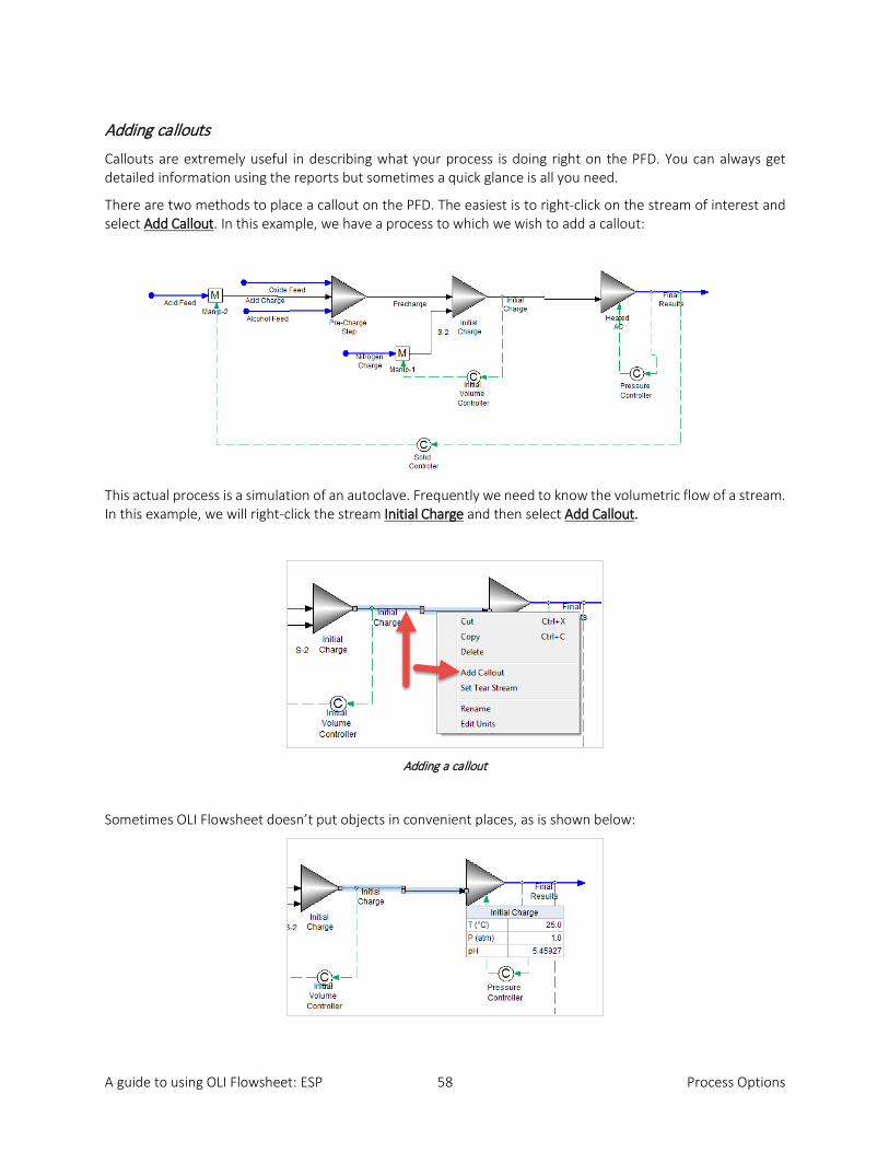
Adding callouts
Callouts are extremely useful in describing what your process is doing right on the PFD. You can always get detailed information using the reports but sometimes a quick glance is all you need.
There are two methods to place a callout on the PFD. The easiest is to right-click on the stream of interest and select Add Callout. In this example, we have a process to which we wish to add a callout:
This actual process is a simulation of an autoclave. Frequently we need to know the volumetric flow of a stream. In this example, we will right-click the stream Initial Charge and then select Add Callout.
Adding a callout
Sometimes OLI Flowsheet doesn’t put objects in convenient places, as is shown below:
A guide to using OLI Flowsheet: ESP 59 Process Options
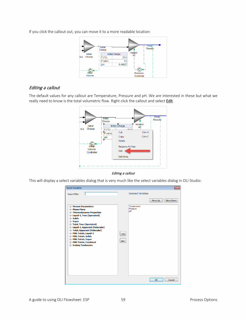
If you click the callout out, you can move it to a more readable location:
Editing a callout
The default values for any callout are Temperature, Pressure and pH. We are interested in these but what we really need to know is the total volumetric flow. Right click the callout and select Edit.
Editing a callout
This will display a select variables dialog that is very much like the select variables dialog in OLI Studio:

A guide to using OLI Flowsheet: ESP 60 Process Options
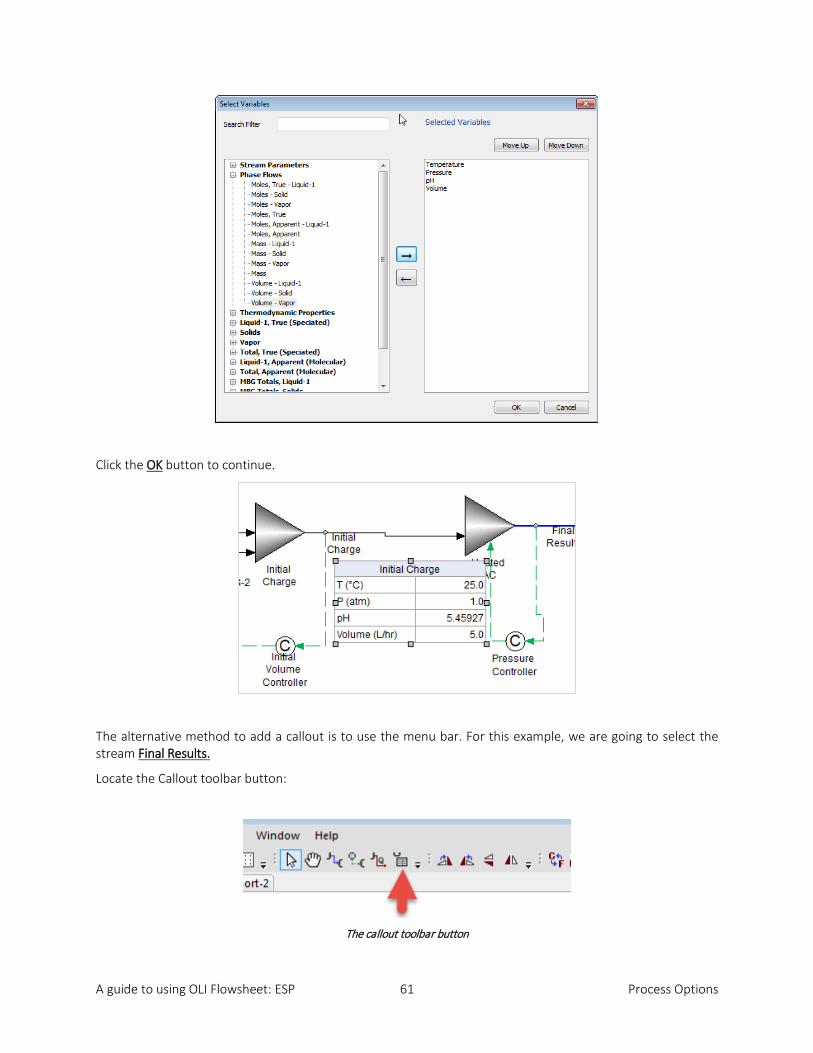
Expand the Phase Flows category and locate the variable Volume:
This variable is the sum of the volumes for all phases. Click the right-arrow key to select it.
Using the right arrow key (you could also double-click the variable to select it)
A guide to using OLI Flowsheet: ESP 61 Process Options
Click the OK button to continue.
The alternative method to add a callout is to use the menu bar. For this example, we are going to select the stream Final Results.
Locate the Callout toolbar button:
The callout toolbar button
A guide to using OLI Flowsheet: ESP 62 Process Options
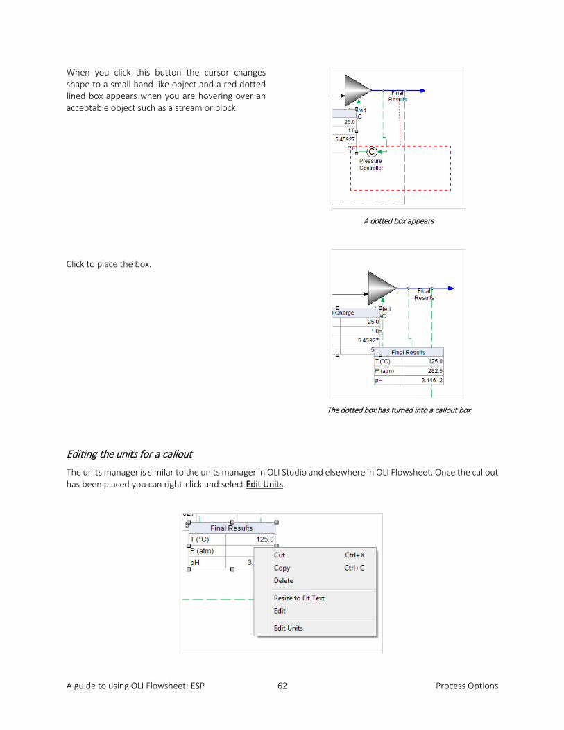
When you click this button the cursor changes shape to a small hand like object and a red dotted lined box appears when you are hovering over an acceptable object such as a stream or block.
Click to place the box.
A dotted box appears
The dotted box has turned into a callout box
Editing the units for a callout
The units manager is similar to the units manager in OLI Studio and elsewhere in OLI Flowsheet. Once the callout has been placed you can right-click and select Edit Units.

A guide to using OLI Flowsheet: ESP 63 Process Options
This will bring up the initial edit units dialog:
Normally for a callout we do not need to make global changes. For this example, we are going to change the temperature units from degrees centigrade to Fahrenheit. Click the Customize button.
A guide to using OLI Flowsheet: ESP 64 Process Options
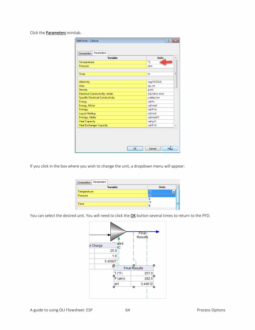
Click the Parameters minitab.
If you click in the box where you wish to change the unit, a dropdown menu will appear:
You can select the desired unit. You will need to click the OK button several times to return to the PFD.

A guide to using OLI Flowsheet: ESP 65 Process Options
Copy and Paste a callout
Once you are satisfied with the parameters and units that you want to show in your callout, you can easily copy and paste on a different stream where you want to see the same variables. This reduces the time to make the customized callouts for different streams.
To do this select the callout that you want to replicate, right click, and select copy.
Then, select the stream where you want to place the callout, and select Paste Callout.

A guide to using OLI Flowsheet: ESP 66 Process Options
The same information and units have been transferred to a different stream.

A guide to using OLI Flowsheet: ESP 67 Process Options
Process Options The Properties Panel has two tabs. The Definition Tab has seven process options. The general tab contains the information specified by the user about the name of the application being built.
Optional Properties This section has the optional properties that can be calculated while running the simulation. The screen lets users choose from an option of a dropdown if they want to enable or disable the calculation of that property. Following is the list of available properties.
To enable the calculation of any of the properties, click on the drop-down arrow and select Yes.
Recycles When this facility is selected, an analysis for process recycle streams is done automatically and, if recycle exists, the user can choose from several options to define the tear stream and recycle convergence.

A guide to using OLI Flowsheet: ESP 68 Process Options
Tear Stream: When clicking Select, in Tear Streams in the recycle options, a new window will open.
In the previous window a suggested tear stream is given, however the user can specify a custom tear stream.
Convergence options can be specified after selecting a tear stream are as follows:
Convergence Method: Three different convergence method are available:
1. Wegstein 2. Newton 3. Avg. Wegstein
A guide to using OLI Flowsheet: ESP 69 Process Options
A brief explanation of how these methods work is given below:
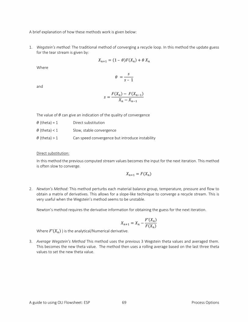
1. Wegstein’s method: The traditional method of converging a recycle loop. In this method the update guess for the tear stream is given by:
𝑋𝑋𝑛𝑛+1 = (1 – 𝜃𝜃)𝐹𝐹(𝑋𝑋𝑛𝑛) + 𝜃𝜃 𝑋𝑋𝑛𝑛
Where
𝜃𝜃 =𝑠𝑠
𝑠𝑠 – 1
and
𝑠𝑠 =𝐹𝐹(𝑋𝑋𝑛𝑛)− 𝐹𝐹(𝑋𝑋𝑛𝑛−1)
𝑋𝑋𝑛𝑛 − 𝑋𝑋𝑛𝑛−1
The value of 𝜃𝜃 can give an indication of the quality of convergence
𝜃𝜃 (theta) = 1 Direct substitution
𝜃𝜃 (theta) < 1 Slow, stable convergence
𝜃𝜃 (theta) > 1 Can speed convergence but introduce instability
Direct substitution:
In this method the previous computed stream values becomes the input for the next iteration. This method is often slow to converge.
𝑋𝑋𝑛𝑛+1 = 𝐹𝐹(𝑋𝑋𝑛𝑛)
2. Newton’s Method: This method perturbs each material balance group, temperature, pressure and flow to obtain a matrix of derivatives. This allows for a slope-like technique to converge a recycle stream. This is very useful when the Wegstein’s method seems to be unstable. Newton’s method requires the derivative information for obtaining the guess for the next iteration.
𝑋𝑋𝑛𝑛+1 = 𝑋𝑋𝑛𝑛 −𝐹𝐹’(𝑋𝑋𝑛𝑛)𝐹𝐹(𝑋𝑋𝑛𝑛)
Where 𝐹𝐹’(𝑋𝑋𝑛𝑛) ) is the analytical/Numerical derivative.
3. Average Wegstein’s Method This method uses the previous 3 Wegstein theta values and averaged them. This becomes the new theta value. The method then uses a rolling average based on the last three theta values to set the new theta value.

A guide to using OLI Flowsheet: ESP 70 Process Options
Max Iterations: Change the default number of iterations that will be performed before a non-convergent case will be terminated.
Not Converged Rule: The choice to continue or stop when a loop does not converge.
Temperature Tolerance (⁰C): Temperature tolerance that determines when the case converges.
Flow Tolerance: Flow tolerance that determined when the case converges.
Restart Options This facility gives the user the option of initializing a recycle stream or a Multi-stage process block with the results from the previous case run.
Molecular Conversion Weights The solver uses weight factors to convert true (speciated) composition to apparent (molecular) composition. If individual weight factors are specified, the component with the bigger number will be favored in converting to molecular flows.

A guide to using OLI Flowsheet: ESP 71 Process Options
Liq-2 Key Component
In the MSE framework, the selected key component will determine the liquid-1 and liquid-2 phase split in the case when only a single liquid phase forms. When the mole fraction of the selected component in liquid phase is more than the specified threshold value, the liquid phase will be treated as the liquid-2 phase. The Liq-2 key component options lets a user choose their own key component from a chemistry model.
Calculation Aids
One of the current calculation aids are to enable trace, This option will create a file with the extension .oue and will contain a detailed convergence history for all Process Blocks. This is useful in determining probable causes for the nonconvergence of Process Block calculations.
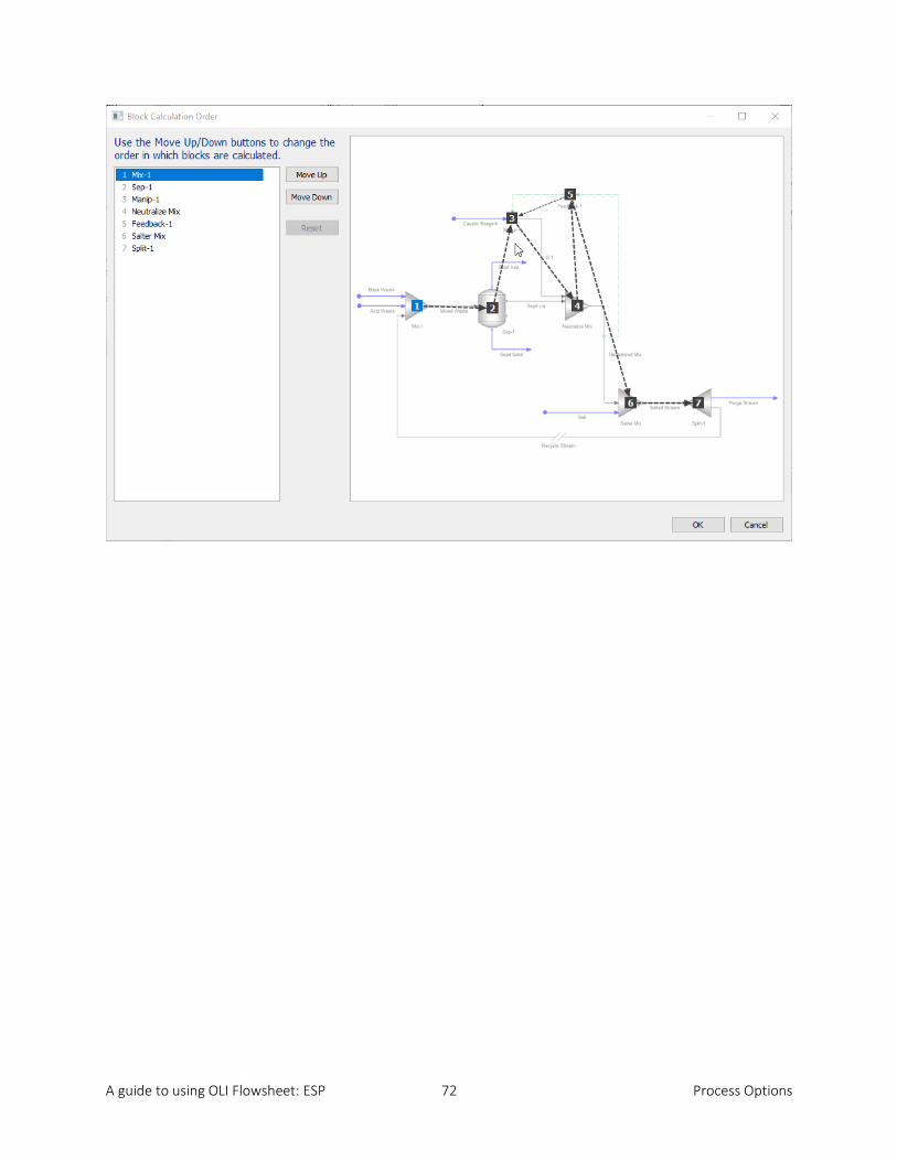
Block Calculation Order
This option will allow the user to specify the order of the blocks to be calculated. It will also allow the choice of executing only part of the process.
The user can change the order of the process by using the Move Up or Move Down Buttons.
A guide to using OLI Flowsheet: ESP 72 Process Options

A guide to using OLI Flowsheet: ESP 73 Reports
Chapter 3. Reports
Let us consider the pH Neutralization with Feedback control and recycle:
In the Report Tab, we have the following options:
• Add a Stream Report • Add a Block Report • Add Multi-Stream Report • Add Overall Process Balance Report • Customize • Export
Stream Report
When using the Stream Report, the user can select a stream for analyzing its properties. Just use the drop-down arrow to select the desired stream:
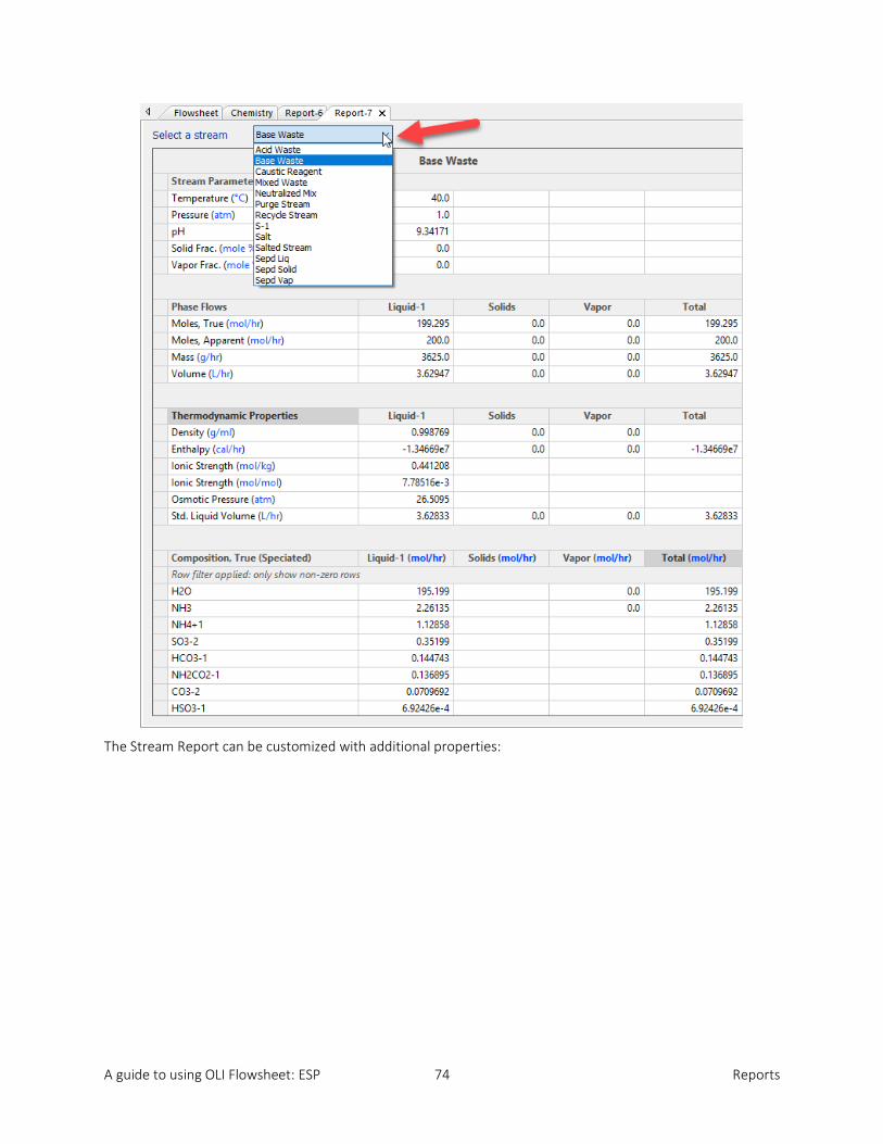
A guide to using OLI Flowsheet: ESP 74 Reports
The Stream Report can be customized with additional properties:

A guide to using OLI Flowsheet: ESP 75 Reports
Block Report
The block report allows the user to view the general information for a specific block. Additionally, the information shown in this table can also be customized.
Multi-stream Report
The Multi-Stream Report gives us the advantage of showing information of different streams for comparison purposes. You can add either all streams of the streams of interest.
To add an additional stream, you need to click in the drop-down arrow, and select the stream of interest, as is shown in the image below:

A guide to using OLI Flowsheet: ESP 76 Reports
Overall Process Balance Report
The overall process balance report shows the information of all inlets and outlets of the process, and information calculated for different blocks.
A material balance group table is also displayed.
The information of the this, report (and all the reports previously explained), can be exported in a .csv file, for posterior analysis in Excel.
A guide to using OLI Flowsheet: ESP 77 Chemistry Models
Chapter 4. Chemistry Models
Overview
In most cases, the user defines a chemistry model by simply entering the names of the chemicals to be covered by the model and the software does the rest. However, this chapter describes all the advanced facilities available to the user.
This section describes in detail the requirements to build a Chemistry Model. The Chemistry Model is important as it describes the specific chemical species and chemical equilibria involved in the application being considered.
The building of a basic Chemistry Model is a quick and simple operation. It is also an essential requirement for the modeling of an electrolyte system. Generally, from a user statement of molecular chemical species, a model is automatically created by the software. This file contains a list of the chemical species in each phase (i.e., vapor, aqueous molecules and ions, and anhydrous and hydrated solids) and the corresponding thermodynamic phase and aqueous speciation equilibrium relationships for the system.
For many OLI applications, this created model is all that is needed to describe the chemistry of the system. However, if required, the model can be augmented by the user to include chemical reaction kinetics, and surface phenomena.
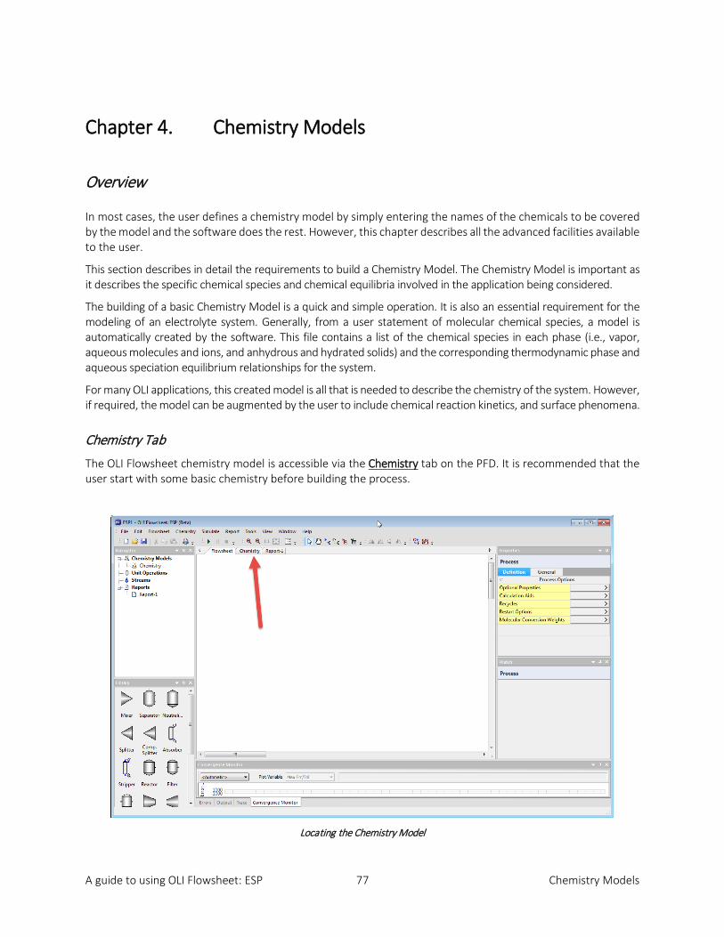
Chemistry Tab
The OLI Flowsheet chemistry model is accessible via the Chemistry tab on the PFD. It is recommended that the user start with some basic chemistry before building the process.
Locating the Chemistry Model

A guide to using OLI Flowsheet: ESP 78 Chemistry Models
Clicking on the Chemistry tab will display the options for the chemistry model.
We start on the default tab Databanks. Here we will modify the data-sets used for this process if required.
Thermodynamic Framework
The user can choose between the default Aqueous (H+ Ion) framework or the MSE (H3O+ Ion) framework.
The default version of the thermodynamic framework is the Aqueous (H+ Ion) framework (also known as AQ Framework).
Databanks
The default databank for each thermodynamic framework is shown. The user cannot make any modifications to the default databank. For the AQ thermodynamic framework, the default databank is Public. For the MSE thermodynamic framework the default databank is MSEPUB.
The add button allows the user to add additional databanks to the process.
A guide to using OLI Flowsheet: ESP 79 Chemistry Models
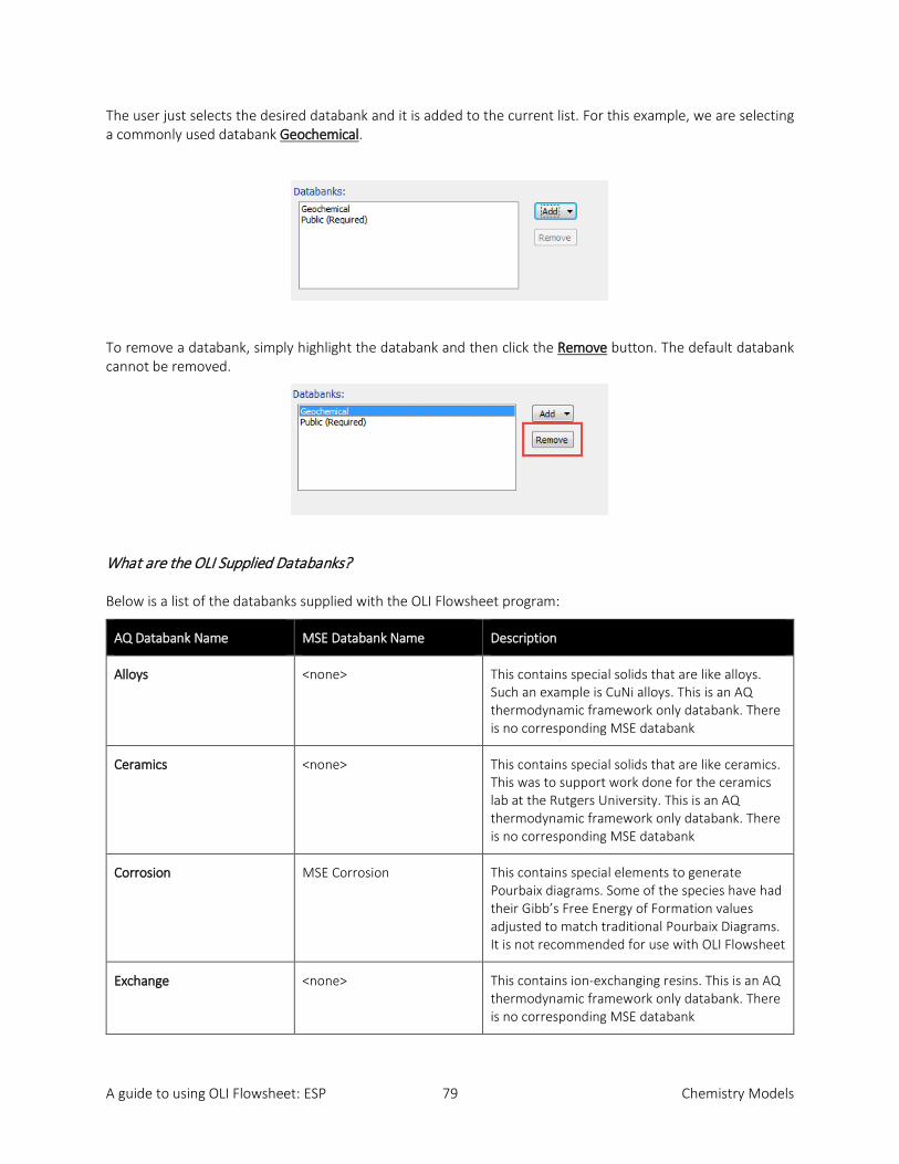
The user just selects the desired databank and it is added to the current list. For this example, we are selecting a commonly used databank Geochemical.
To remove a databank, simply highlight the databank and then click the Remove button. The default databank cannot be removed.
What are the OLI Supplied Databanks?
Below is a list of the databanks supplied with the OLI Flowsheet program:
AQ Databank Name MSE Databank Name Description
Alloys <none> This contains special solids that are like alloys. Such an example is CuNi alloys. This is an AQ thermodynamic framework only databank. There is no corresponding MSE databank
Ceramics <none> This contains special solids that are like ceramics. This was to support work done for the ceramics lab at the Rutgers University. This is an AQ thermodynamic framework only databank. There is no corresponding MSE databank
Corrosion MSE Corrosion This contains special elements to generate Pourbaix diagrams. Some of the species have had their Gibb’s Free Energy of Formation values adjusted to match traditional Pourbaix Diagrams. It is not recommended for use with OLI Flowsheet
Exchange <none> This contains ion-exchanging resins. This is an AQ thermodynamic framework only databank. There is no corresponding MSE databank

A guide to using OLI Flowsheet: ESP 80 Chemistry Models
Geochemical MSE Geochemical This contains minerals that are primarily found in geothermal applications. These minerals typically do not reform under traditional chemical process conditions.
Low Temperature <none> This databank contains minerals that form below 0oC (273.15 K). This is an AQ thermodynamic framework only databank. There is no corresponding MSE databank
Surface Complexation Capacitance Model
<none> This databank contains surface species following Dzombak’s model for capacitance. This is an AQ thermodynamic framework only databank. There is no corresponding MSE databank
Surface Complexation Double Layer Model
XSC Databank This databank contains surface species following Dzombak’s model for Double-layers capacitance.
Surface Complexation Non-Electrostatic Model
<none> This databank contains surface species following Dzombak’s model for non-electrostatic interactions. This is an AQ thermodynamic framework only databank. There is no corresponding MSE databank
Surface Complexation Triple Layer Model
<none> This databank contains surface species following Dzombak’s model for Triple-layers. This is an AQ thermodynamic framework only databank. There is no corresponding MSE databank
<none> MSE Urea This databank contains surface species that support high temperature formation of urea. It is not recommended unless urea is known to form from NH3 and CO2. Generally, such formations are kinetically limited. This is an MSE thermodynamic framework only databank. There is no corresponding AQ databank
A guide to using OLI Flowsheet: ESP 81 Chemistry Models
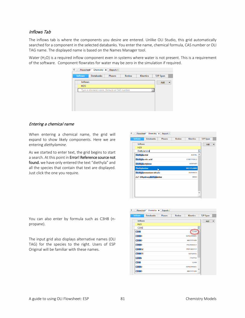
Inflows Tab
The inflows tab is where the components you desire are entered. Unlike OLI Studio, this grid automatically searched for a component in the selected databanks. You enter the name, chemical formula, CAS number or OLI TAG name. The displayed name is based on the Names Manager tool.
Water (H2O) is a required inflow component even in systems where water is not present. This is a requirement of the software. Component flowrates for water may be zero in the simulation if required.
Entering a chemical name
When entering a chemical name, the grid will expand to show likely components. Here we are entering diethylamine.
As we started to enter text, the grid begins to start a search. At this point in Error! Reference source not found. we have only entered the text “diethyla” and all the species that contain that text are displayed. Just click the one you require.
You can also enter by formula such as C3H8 (n-propane).
The input grid also displays alternative names (OLI TAG) for the species to the right. Users of ESP Original will be familiar with these names.

A guide to using OLI Flowsheet: ESP 82 Chemistry Models
Add Button
The Add Button allows the user to add different types of chemistry. The user can add a Pseudo-Component or a Petroleum Assay.
Adding a Pseudo-Component
Pseudo-components are user created species which simulate portions of petroleum products. Typically, a user will have some analysis of an oil sample such as assay data (boiling point data and the like) which will be broken down into individual pseudo-components. This task will be discussed in the next section. Alternatively, the user may have the data for each pseudo-component derived from other sources. This type of data can be entered via this menu item.
Select Add Pseudo-component
We have several items to enter for each individual pseudo-component. The first item is a name. Enter a name in the <Type a Name box. This name must be unique to the model and cannot be the name of a component already in the OLI software (the program will warn you accordingly). Typically, the pseudo-component name uses the letters “PC” and some number. Here we will use the name PC1.

A guide to using OLI Flowsheet: ESP 83 Chemistry Models
Thermo Method
We now need to define a thermodynamic method to convert the entered data to a thermodynamic entity. The default method is API-8 (American Petroleum Institute Method 8).
OLI Flowsheet supports the following methods: • API-8 (default) • API-5 • Cavett • Kessler
A more detailed explanation of each method is given below:
API 8 and 5 Uses the specific gravity to estimate the critical parameters. The specific gravity, if not entered, can be estimated from the API gravity or the Watson K. The boiling points are taken from the assay data.
Cavett This method uses the API gravity method to determine the critical properties. The API gravity, if not entered can be estimated from the actual specific gravity or the Watson K. The boiling points for the pseudo-components are taken from the assay.
Lee-Kesler This method uses the Watson K and the specific gravity (which can be estimated via the Watson K) to determine the critical parameters.
The user may enter any two of the three parameters listed in the figure Error! Reference source not found.: Normal Boiling Point, Specific Gravity, And Molecular Weight. The parameter not entered will be calculated using the selected thermo method. If all three parameters are entered, then only the parameters Normal Boiling Point and Specific Gravity will be used.
Adding an Assay
Assays are characteristics of oil samples. Typically, some sort of distillation data has been collected and will be entered into the software. This distillation data will be “Cut” into individual pseudo-components.
Click the Add Assay menu item.
As with pseudo-components a name is required that must be unique for this document. The name may not be the same as any component currently in the OLI software (the software will check for this). Typically, a name such as “AS” is used with a number appended (such as AS1). The name is limited to 5 characters and the program will enforce this rule.
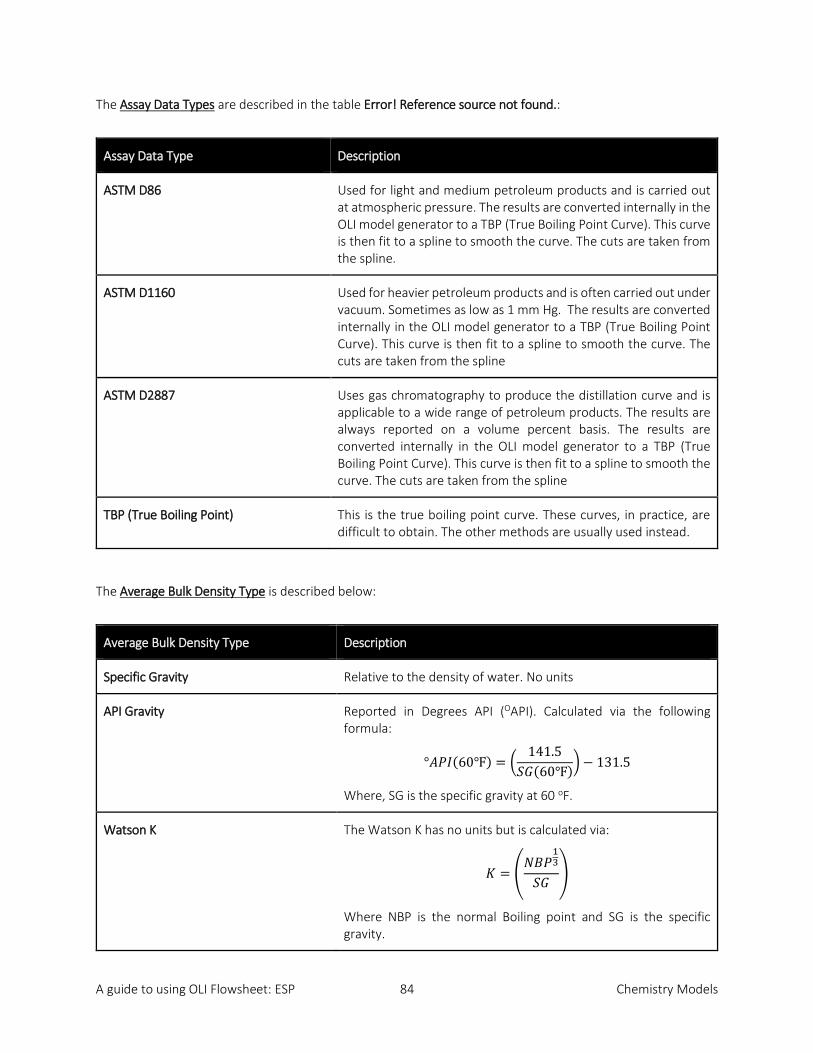
A guide to using OLI Flowsheet: ESP 84 Chemistry Models
The Assay Data Types are described in the table Error! Reference source not found.:
Assay Data Type Description
ASTM D86 Used for light and medium petroleum products and is carried out at atmospheric pressure. The results are converted internally in the OLI model generator to a TBP (True Boiling Point Curve). This curve is then fit to a spline to smooth the curve. The cuts are taken from the spline.
ASTM D1160 Used for heavier petroleum products and is often carried out under vacuum. Sometimes as low as 1 mm Hg. The results are converted internally in the OLI model generator to a TBP (True Boiling Point Curve). This curve is then fit to a spline to smooth the curve. The cuts are taken from the spline
ASTM D2887 Uses gas chromatography to produce the distillation curve and is applicable to a wide range of petroleum products. The results are always reported on a volume percent basis. The results are converted internally in the OLI model generator to a TBP (True Boiling Point Curve). This curve is then fit to a spline to smooth the curve. The cuts are taken from the spline
TBP (True Boiling Point) This is the true boiling point curve. These curves, in practice, are difficult to obtain. The other methods are usually used instead.
The Average Bulk Density Type is described below:
Average Bulk Density Type Description
Specific Gravity Relative to the density of water. No units
API Gravity Reported in Degrees API (OAPI). Calculated via the following formula:
°𝐴𝐴𝐴𝐴𝐴𝐴(60℉) = �141.5
𝑆𝑆𝑆𝑆(60℉)� − 131.5
Where, SG is the specific gravity at 60 oF.
Watson K The Watson K has no units but is calculated via:
𝐾𝐾 = �𝑁𝑁𝑁𝑁𝐴𝐴
13
𝑆𝑆𝑆𝑆 �
Where NBP is the normal Boiling point and SG is the specific gravity.
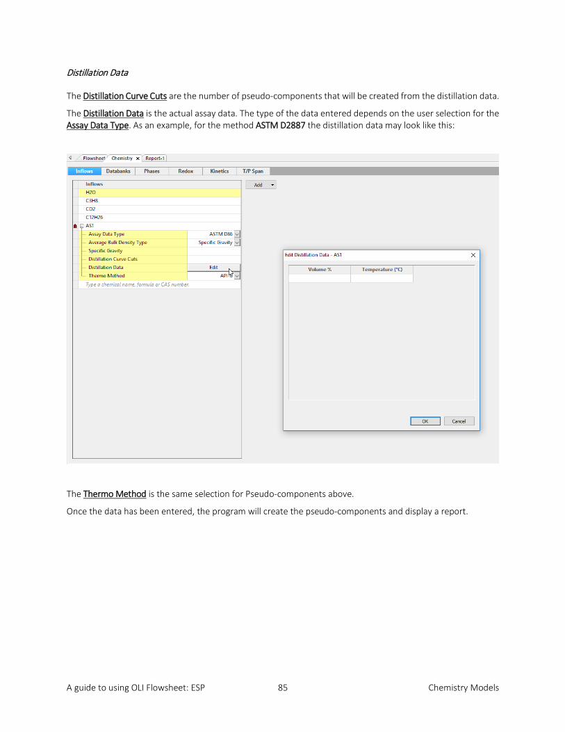
A guide to using OLI Flowsheet: ESP 85 Chemistry Models
Distillation Data
The Distillation Curve Cuts are the number of pseudo-components that will be created from the distillation data.
The Distillation Data is the actual assay data. The type of the data entered depends on the user selection for the Assay Data Type. As an example, for the method ASTM D2887 the distillation data may look like this:
The Thermo Method is the same selection for Pseudo-components above.
Once the data has been entered, the program will create the pseudo-components and display a report.

A guide to using OLI Flowsheet: ESP 86 Chemistry Models
Phases Tab The Phases Tab allows the user to modify the default phase behavior. In this example we have created the follow chemistry using the Inflows Tab.
Click on the Phases tab.
OLI considers the possibility of a vapor phase, second liquid phase (also referred to as an organic phase) and multiple solid phases. OLI always considers a water-rich phase referred to as Liquid 1.
The user can enable or disable phases by unchecking the phase box. In figure above, all phases have been enabled.
The user may also disable individual solid phases if they are known not to form under the conditions specified in the flowsheet. The solids are grouped by material codes and can be expanded by section.
The All group has all the solid displayed.
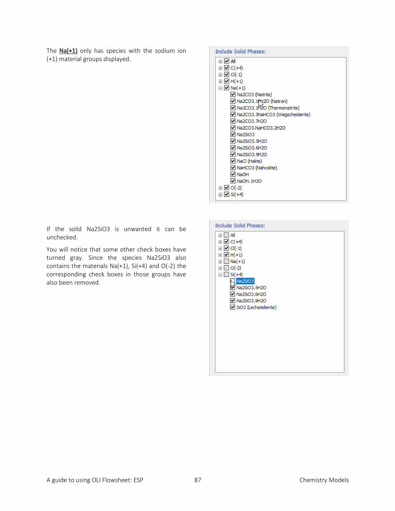
A guide to using OLI Flowsheet: ESP 87 Chemistry Models
The Na(+1) only has species with the sodium ion (+1) material groups displayed.
If the solid Na2SiO3 is unwanted it can be unchecked.
You will notice that some other check boxes have turned gray. Since the species Na2SiO3 also contains the materials Na(+1), Si(+4) and O(-2) the corresponding check boxes in those groups have also been removed.
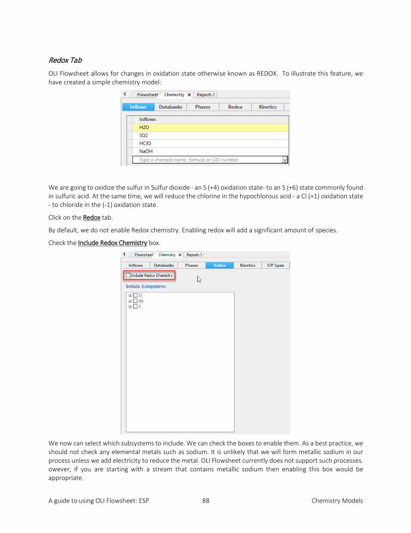
A guide to using OLI Flowsheet: ESP 88 Chemistry Models
Redox Tab
OLI Flowsheet allows for changes in oxidation state otherwise known as REDOX. To illustrate this feature, we have created a simple chemistry model:
We are going to oxidize the sulfur in Sulfur dioxide - an S (+4) oxidation state- to an S (+6) state commonly found in sulfuric acid. At the same time, we will reduce the chlorine in the hypochlorous acid - a Cl (+1) oxidation state - to chloride in the (-1) oxidation state.
Click on the Redox tab.
By default, we do not enable Redox chemistry. Enabling redox will add a significant amount of species.
Check the Include Redox Chemistry box.
We now can select which subsystems to include. We can check the boxes to enable them. As a best practice, we should not check any elemental metals such as sodium. It is unlikely that we will form metallic sodium in our process unless we add electricity to reduce the metal. OLI Flowsheet currently does not support such processes. owever, if you are starting with a stream that contains metallic sodium then enabling this box would be appropriate.
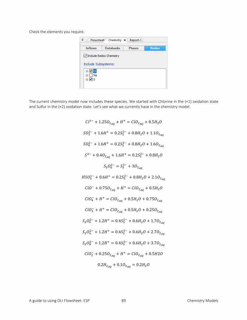
A guide to using OLI Flowsheet: ESP 89 Chemistry Models
Check the elements you require.
The current chemistry model now includes these species. We started with Chlorine in the (+1) oxidation state and Sulfur in the (+2) oxidation state. Let’s see what we currently have in the chemistry model.
𝐶𝐶𝑙𝑙1− + 1.25𝑂𝑂2𝐴𝐴𝐴𝐴 +𝐻𝐻+ = 𝐶𝐶𝑙𝑙𝑂𝑂2𝐴𝐴𝐴𝐴 + 0.5𝐻𝐻2𝑂𝑂
𝑆𝑆𝑂𝑂32− + 1.6𝐻𝐻+ = 0.2𝑆𝑆52− + 0.8𝐻𝐻2𝑂𝑂 + 1.1𝑂𝑂2𝐴𝐴𝐴𝐴
𝑆𝑆𝑂𝑂42− + 1.6𝐻𝐻+ = 0.2𝑆𝑆52− + 0.8𝐻𝐻2𝑂𝑂 + 1.6𝑂𝑂2𝐴𝐴𝐴𝐴
𝑆𝑆2− + 0.4𝑂𝑂2𝐴𝐴𝐴𝐴 + 1.6𝐻𝐻+ = 0.2𝑆𝑆52− + 0.8𝐻𝐻2𝑂𝑂
𝑆𝑆5𝑂𝑂62− = 𝑆𝑆52− + 3𝑂𝑂2𝐴𝐴𝐴𝐴
𝐻𝐻𝑆𝑆𝑂𝑂51− + 0.6𝐻𝐻+ = 0.2𝑆𝑆52− + 0.8𝐻𝐻2𝑂𝑂 + 2.1𝑂𝑂2𝐴𝐴𝐴𝐴
𝐶𝐶𝑙𝑙𝑂𝑂− + 0.75𝑂𝑂2𝐴𝐴𝐴𝐴 + 𝐻𝐻+ = 𝐶𝐶𝑙𝑙𝑂𝑂2𝐴𝐴𝐴𝐴 + 0.5𝐻𝐻2𝑂𝑂
𝐶𝐶𝑙𝑙𝑂𝑂4− + 𝐻𝐻+ = 𝐶𝐶𝑙𝑙𝑂𝑂2𝐴𝐴𝐴𝐴 + 0.5𝐻𝐻2𝑂𝑂 + 0.75𝑂𝑂2𝐴𝐴𝐴𝐴
𝐶𝐶𝑙𝑙𝑂𝑂3− + 𝐻𝐻+ = 𝐶𝐶𝑙𝑙𝑂𝑂2𝐴𝐴𝐴𝐴 + 0.5𝐻𝐻2𝑂𝑂 + 0.25𝑂𝑂2𝐴𝐴𝐴𝐴
𝑆𝑆2𝑂𝑂42− + 1.2𝐻𝐻+ = 0.4𝑆𝑆52− + 0.6𝐻𝐻2𝑂𝑂 + 1.7𝑂𝑂2𝐴𝐴𝐴𝐴
𝑆𝑆2𝑂𝑂62− + 1.2𝐻𝐻+ = 0.4𝑆𝑆52− + 0.6𝐻𝐻2𝑂𝑂 + 2.7𝑂𝑂2𝐴𝐴𝐴𝐴
𝑆𝑆2𝑂𝑂82− + 1.2𝐻𝐻+ = 0.4𝑆𝑆52− + 0.6𝐻𝐻2𝑂𝑂 + 3.7𝑂𝑂2𝐴𝐴𝐴𝐴
𝐶𝐶𝑙𝑙𝑂𝑂2− + 0.25𝑂𝑂2𝐴𝐴𝐴𝐴 + 𝐻𝐻+ = 𝐶𝐶𝑙𝑙𝑂𝑂2𝐴𝐴𝐴𝐴 + 0.5𝐻𝐻2𝑂𝑂
0.2𝐻𝐻2𝐴𝐴𝐴𝐴 + 0.1𝑂𝑂2𝐴𝐴𝐴𝐴 = 0.2𝐻𝐻2𝑂𝑂
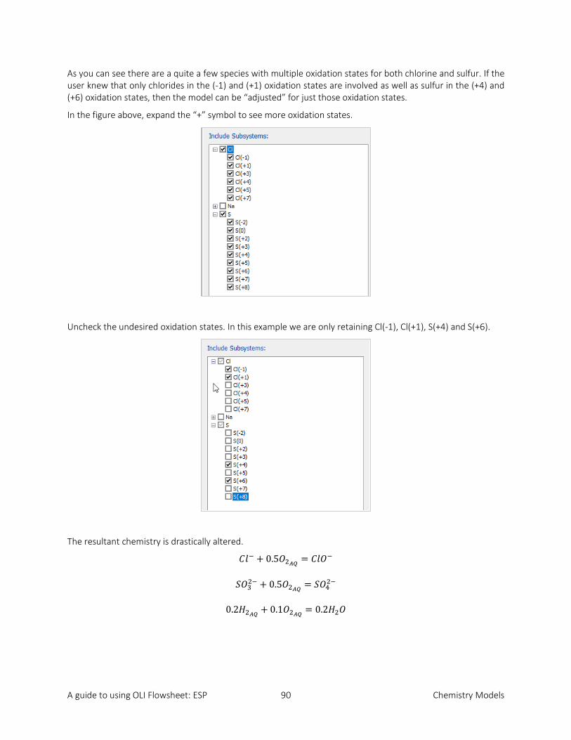
A guide to using OLI Flowsheet: ESP 90 Chemistry Models
As you can see there are a quite a few species with multiple oxidation states for both chlorine and sulfur. If the user knew that only chlorides in the (-1) and (+1) oxidation states are involved as well as sulfur in the (+4) and (+6) oxidation states, then the model can be “adjusted” for just those oxidation states.
In the figure above, expand the “+” symbol to see more oxidation states.
Uncheck the undesired oxidation states. In this example we are only retaining Cl(-1), Cl(+1), S(+4) and S(+6).
The resultant chemistry is drastically altered.
𝐶𝐶𝑙𝑙− + 0.5𝑂𝑂2𝐴𝐴𝐴𝐴 = 𝐶𝐶𝑙𝑙𝑂𝑂−
𝑆𝑆𝑂𝑂32− + 0.5𝑂𝑂2𝐴𝐴𝐴𝐴 = 𝑆𝑆𝑂𝑂42−
0.2𝐻𝐻2𝐴𝐴𝐴𝐴 + 0.1𝑂𝑂2𝐴𝐴𝐴𝐴 = 0.2𝐻𝐻2𝑂𝑂

A guide to using OLI Flowsheet: ESP 91 Chemistry Models
Kinetics Tab
Reaction Kinetics Overview
The OLI thermodynamic framework supports reaction kinetics. Reaction kinetics can be defined in standard Arrhenius terms or in terms defined by the user. There are only two different unit operations that support reaction kinetics: REACTOR unit and Multistage COLUMNS such as STRIPPERS and ABSORBERS.
Reaction Types
There are two general types of reaction kinetics:
Type 1: Change in material balance codes across the reaction
As an example, consider the following reaction:
𝐶𝐶𝐻𝐻4 + 2𝑂𝑂2 = 𝐶𝐶𝑂𝑂2 + 2𝐻𝐻2𝑂𝑂
The material balance codes across the reaction are:
Species Material Balance Codes
= Species Material Balance Codes
CH4 1001 CO2 25, 1
O2 57 H2O 1, 21
Due to the material balance code changes across this reaction there will be no equilibrium reaction or any combination of equilibrium reaction to produce this reaction. This assumes that no oxidation/reduction reactions are present in the equilibrium reactions.
In fact, this is a requirement of our kinetic models that kinetics and oxidation/reduction reactions cannot be mixed. You must use all kinetic or all oxidation/reduction, not a mixture of both.
Type 2: No change in material balance codes across the reaction
Consider this reaction:
𝐶𝐶𝐴𝐴𝐶𝐶𝑂𝑂3𝐴𝐴𝐴𝐴𝑃𝑃 = 𝐶𝐶𝐴𝐴𝐴𝐴𝑂𝑂𝑁𝑁 + 𝐶𝐶𝑂𝑂3𝐴𝐴𝑂𝑂𝑁𝑁
The material balance codes across the reaction are:
Species Material Balance Codes
= Species Material Balance Codes
CACO3PPT 6, 25, 21 CAION 6
CO3ION 25, 21

A guide to using OLI Flowsheet: ESP 92 Chemistry Models
The material codes on both sides of the equation are the same. Therefore, the equilibrium model will contain this reaction either directly or as a combination of equilibrium reactions. To include this kinetic reaction, the equilibrium model must be changed to remove the equilibrium between these species. The software will re-write the equilibrium reactions by removing the CACO3PPT from the equilibrium reaction set. Thus, the only way to make or consume CaCO3ppt is by the kinetic reaction. If the user wants to feed CaCO3ppt to the reactor, an additional input has been provided in the interface routine to specify the amount of CaCO3ppt feed. An additional key word has been added to the kinetics section of the model file where the use can specify which species will be removed from the equilibrium calculation.
Kinetics Types
There are two types of kinetics available in OLI Flowsheet. The first is Arrhenius type (also known as Standard type) and the other is User type (also known as SPEC type).
Standard Rate Expressions
In this mode, the rate of reaction is calculated using a standard rate expression. This expression considers both the forward and reverse reaction rates, the individual species reaction orders, and the forward and reverse reaction constants (determined using the Arrhenius Equation).
The standard rate expression is best illustrated by means of an example. Consider the general equation:
𝑎𝑎𝐴𝐴 + 𝑏𝑏𝑁𝑁 + ⋯ = 𝑐𝑐𝐶𝐶 + 𝑑𝑑𝑑𝑑 + ⋯
where: 𝑎𝑎,𝑏𝑏, … 𝑐𝑐,𝑑𝑑 are stoichiometric coefficients.
and: 𝐴𝐴,𝑁𝑁, … are reactant species
𝐶𝐶,𝑑𝑑, … are product species
The standard rate expression is of the form:
𝑅𝑅𝑎𝑎𝑅𝑅𝑅𝑅 = �𝑘𝑘𝑓𝑓𝑎𝑎𝐴𝐴𝑟𝑟1𝑎𝑎𝐵𝐵𝑟𝑟2 …− 𝑘𝑘𝑟𝑟𝑎𝑎𝐶𝐶𝑝𝑝1𝑎𝑎𝐷𝐷
𝑝𝑝2�× 𝑉𝑉𝑉𝑉𝑙𝑙
where:
𝑅𝑅𝑎𝑎𝑅𝑅𝑅𝑅 = Reaction rate �𝑚𝑚𝑚𝑚𝑚𝑚𝑚𝑚𝑚𝑚3ℎ𝑟𝑟
�
ℎ𝑟𝑟
𝑘𝑘𝑓𝑓 = Forward reaction rate constant �𝑚𝑚𝑚𝑚𝑚𝑚𝑚𝑚𝑚𝑚3ℎ𝑟𝑟
�
ℎ𝑟𝑟
𝑘𝑘𝑟𝑟 = Reverse reaction rate constant �𝑚𝑚𝑚𝑚𝑚𝑚𝑚𝑚𝑚𝑚3ℎ𝑟𝑟
�
ℎ𝑟𝑟
𝑎𝑎𝐴𝐴,𝑎𝑎𝐵𝐵, … = Activities of reactant species (unitless)
𝑟𝑟1, 𝑟𝑟2 … = Reaction order of individual reactant species (normally from experimental data. Default is stoichiometric coefficients; a, b, ...)
𝑎𝑎𝐶𝐶 ,𝑎𝑎𝐷𝐷, … = Activities of product species
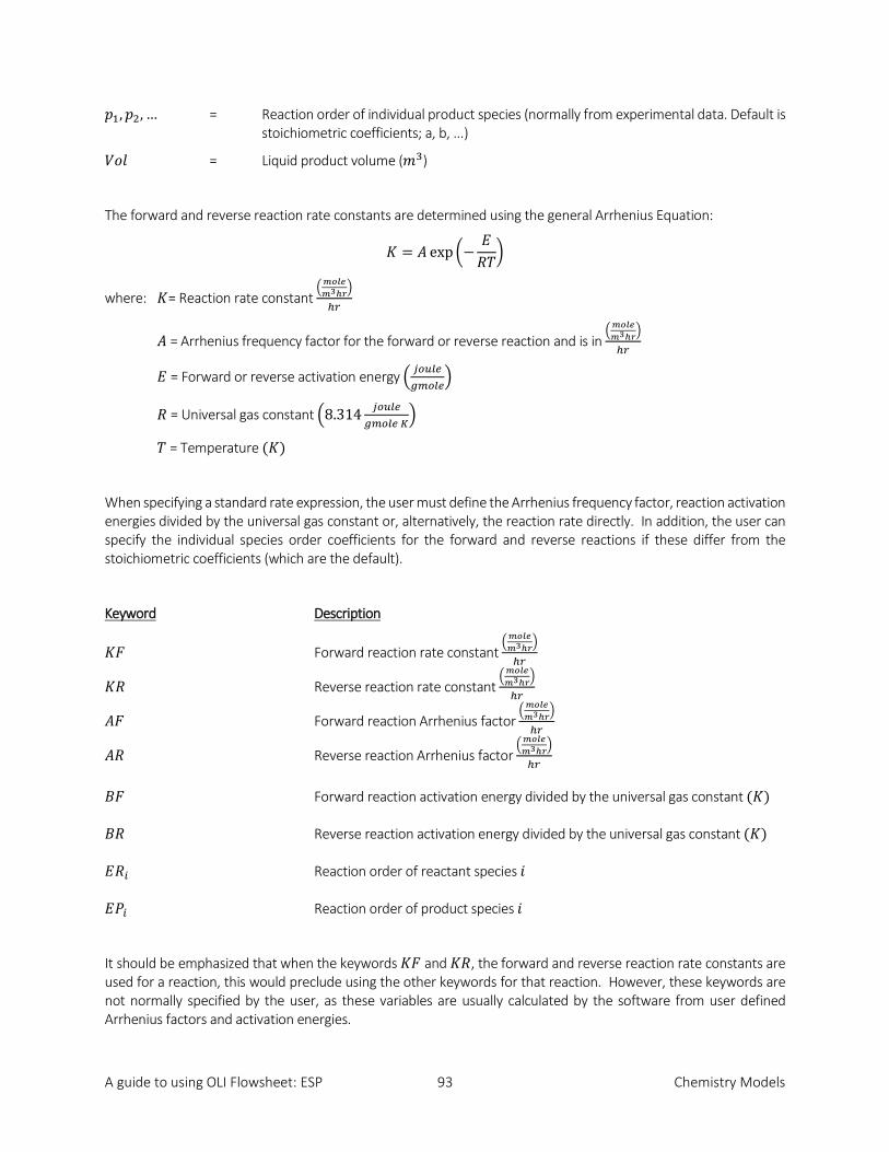
A guide to using OLI Flowsheet: ESP 93 Chemistry Models
𝑝𝑝1,𝑝𝑝2, … = Reaction order of individual product species (normally from experimental data. Default is stoichiometric coefficients; a, b, ...)
𝑉𝑉𝑉𝑉𝑙𝑙 = Liquid product volume (𝑚𝑚3)
The forward and reverse reaction rate constants are determined using the general Arrhenius Equation:
𝐾𝐾 = 𝐴𝐴 exp �−𝐸𝐸𝑅𝑅𝑃𝑃
�
where: 𝐾𝐾= Reaction rate constant �𝑚𝑚𝑚𝑚𝑚𝑚𝑚𝑚𝑚𝑚3ℎ𝑟𝑟
�
ℎ𝑟𝑟
𝐴𝐴 = Arrhenius frequency factor for the forward or reverse reaction and is in �𝑚𝑚𝑚𝑚𝑚𝑚𝑚𝑚𝑚𝑚3ℎ𝑟𝑟
�
ℎ𝑟𝑟
𝐸𝐸 = Forward or reverse activation energy � 𝑗𝑗𝑗𝑗𝑗𝑗𝑗𝑗𝑗𝑗𝑔𝑔𝑔𝑔𝑗𝑗𝑗𝑗𝑗𝑗
�
𝑅𝑅 = Universal gas constant �8.314 𝑗𝑗𝑗𝑗𝑗𝑗𝑗𝑗𝑗𝑗𝑔𝑔𝑔𝑔𝑗𝑗𝑗𝑗𝑗𝑗 𝐾𝐾
�
𝑃𝑃 = Temperature (𝐾𝐾)
When specifying a standard rate expression, the user must define the Arrhenius frequency factor, reaction activation energies divided by the universal gas constant or, alternatively, the reaction rate directly. In addition, the user can specify the individual species order coefficients for the forward and reverse reactions if these differ from the stoichiometric coefficients (which are the default).
Keyword Description
𝐾𝐾𝐹𝐹 Forward reaction rate constant �𝑚𝑚𝑚𝑚𝑚𝑚𝑚𝑚𝑚𝑚3ℎ𝑟𝑟
�
ℎ𝑟𝑟
𝐾𝐾𝑅𝑅 Reverse reaction rate constant �𝑚𝑚𝑚𝑚𝑚𝑚𝑚𝑚𝑚𝑚3ℎ𝑟𝑟
�
ℎ𝑟𝑟
𝐴𝐴𝐹𝐹 Forward reaction Arrhenius factor �𝑚𝑚𝑚𝑚𝑚𝑚𝑚𝑚𝑚𝑚3ℎ𝑟𝑟
�
ℎ𝑟𝑟
𝐴𝐴𝑅𝑅 Reverse reaction Arrhenius factor �𝑚𝑚𝑚𝑚𝑚𝑚𝑚𝑚𝑚𝑚3ℎ𝑟𝑟
�
ℎ𝑟𝑟
𝑁𝑁𝐹𝐹 Forward reaction activation energy divided by the universal gas constant (𝐾𝐾) 𝑁𝑁𝑅𝑅 Reverse reaction activation energy divided by the universal gas constant (𝐾𝐾) 𝐸𝐸𝑅𝑅𝑖𝑖 Reaction order of reactant species 𝑖𝑖 𝐸𝐸𝐴𝐴𝑖𝑖 Reaction order of product species 𝑖𝑖
It should be emphasized that when the keywords 𝐾𝐾𝐹𝐹 and 𝐾𝐾𝑅𝑅, the forward and reverse reaction rate constants are used for a reaction, this would preclude using the other keywords for that reaction. However, these keywords are not normally specified by the user, as these variables are usually calculated by the software from user defined Arrhenius factors and activation energies.
A guide to using OLI Flowsheet: ESP 94 Chemistry Models
When defining the reaction order for a species, the order in which the species appears in the reaction equation must be defined (i.e., subscript i) with a sequential number, for either the reactant or product species. Hence, the first reactant is identified with the number 1, the second, 2 and so on. Similarly, the product species are identified with the integers 1, 2, 3 ... etc.
If any of the keywords are not defined, the software assumes a default value for that variable. These default values are assumed to be zero for the reaction rate constants, Arrhenius factors, and activation energies (divided by the universal gas constant). For the species reaction order coefficients, the reaction stoichiometric values are assumed.
To complete the standard rate expression definition, the reaction temperature and initial reactant molality are included in the process stream composition definition.
You can review a full example for the Standard Reaction Kinetics on page 148 using a reactor block.
Non-Standard (User Defined) Reaction Kinetics
The user can define his/her own reaction kinetics.
You can review a full example for Non-standard Reaction Kinetics on page 155.
T/P Span
The T/P Span is for the temperature and pressure limits on the equation of state for the model. This only applies to the AQ thermodynamic framework. It is generally recommended that these values not be altered. These values are ignored for both the MSE and MSE-SRK thermodynamic frameworks.
History Lesson
Before 1990, OLI used a mixture of different thermodynamic frameworks to represent the standard state (equilibrium constants). Starting in 1990, OLI migrated to the Helgeson Equation of State3. This equation of state provided a consistent representation of the standard state for species in water up to 374 oC and 5000 atmospheres.
The problem in the 1990’s is that computers were slow and the direct method of calculating the equation of state was computationally intensive. Marshall Rafal (OLI – retired) observed that since the equation of state was only a function of temperature and pressure that the equilibrium constants could be pre-fit before calculation time. A matrix of temperatures (T span) and pressures (P span) were generated and then fit to a polynomial equation.
Evaluation of this polynomial is very fast, even in the 1990’s, so it is used for the AQ thermodynamic framework. This was too inaccurate for the MSE thermodynamic framework and all values in the T/P are ignored.
3 Helgeson, Harold C., Kirkham, David H and Flowers, George, C. “Theoretical Prediction of the Thermodynamic Behavior of Aqueous Electrolytes at High Pressures and Temperatures – Parts I Though IV.” American Journal of Science (1982)
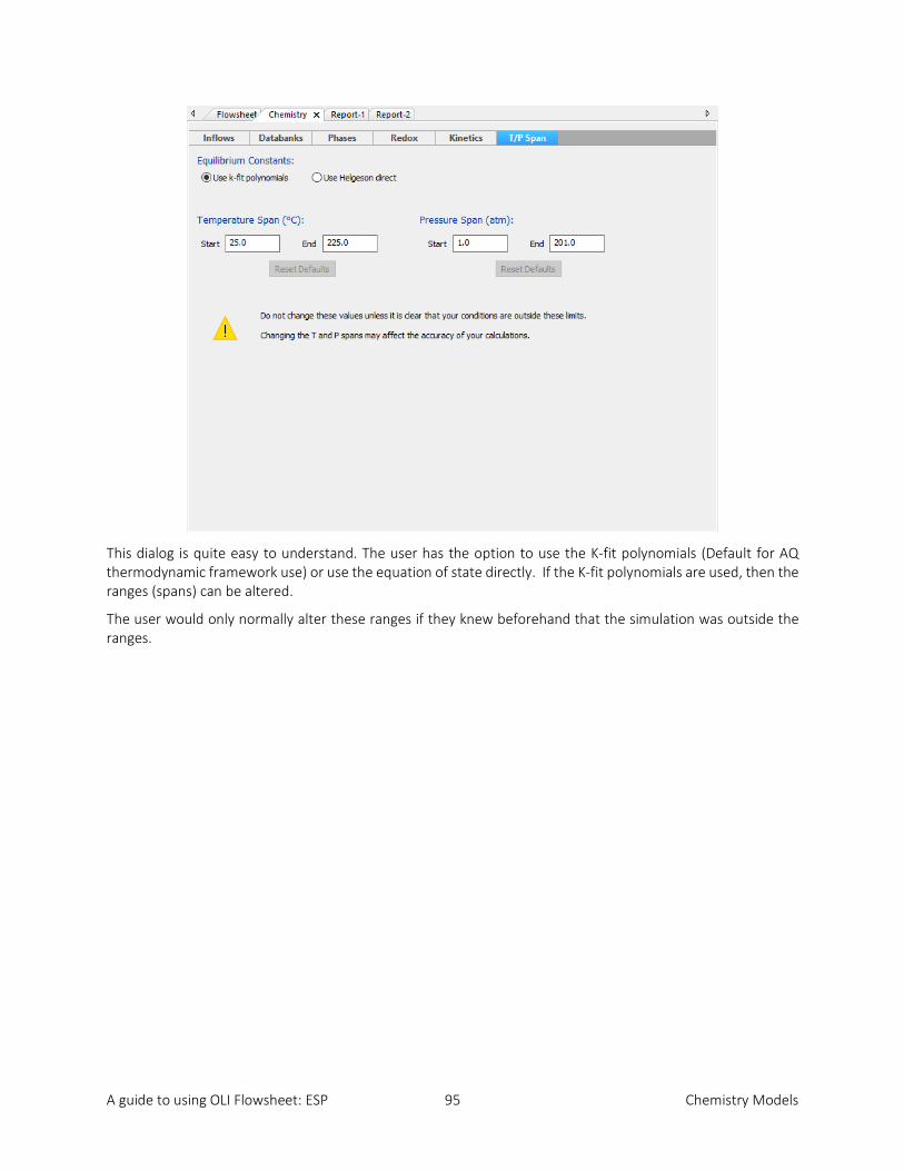
A guide to using OLI Flowsheet: ESP 95 Chemistry Models
This dialog is quite easy to understand. The user has the option to use the K-fit polynomials (Default for AQ thermodynamic framework use) or use the equation of state directly. If the K-fit polynomials are used, then the ranges (spans) can be altered.
The user would only normally alter these ranges if they knew beforehand that the simulation was outside the ranges.

A guide to using OLI Flowsheet: ESP 96 Process Modeling
Chapter 5. Process Modeling
Overview
This section is a detailed guide to the use of unit operations, called Process Blocks, and for the use of the steady-state flowsheet simulation facilities provided via OLI Flowsheet: ESP. This chapter contains a brief overview and detailed specifications of the OLI Flowsheet: ESP Process Blocks. Limitations and guidelines for individual units are included.
By selecting pertinent unit operations, a complete process can be modeled by combining individual process blocks into a process flowsheet to describe the process.
Unit Operations/Blocks and Controllers
The current blocks available in OLI Flowsheet: ESP are:
1. Mixer 2. Separator 3. Neutralizer 4. Splitter 5. Component Splitter 6. Absorber 7. Stripper 8. Extractor 9. Reactor 10. Filter 11. Settler 12. RO Membranes 13. Compressor 14. Turbine 15. Heat Exchanger 16. Incinerator 17. Feedback controller 18. Feedforward controller 19. Manipulator 20. Pump

A guide to using OLI Flowsheet: ESP 97 Process Modeling
Unit Operations/Blocks and Controllers Summary Descriptions
1. Mixer
A conventional Process Block which allows mixing of several (2-7) inlet streams adiabatically. The resulting phase separation and speciation within each phase is also evaluated.
2. Separator
A conventional Process Block which allows up to 7 inlets to be separated into distinct physical phases. Suspended solids, entrained liquid, dissolved vapor and dissolved liquid can be specified. An equilibrium will be performed adiabatically.
3. Neutralizer
An Environmental Process Block which allows a specified stream to be neutralized, either by adiabatically mixing the inlet streams, or by varying one of the inlet streams to meet a specified pH point.

A guide to using OLI Flowsheet: ESP 98 Process Modeling
4. Splitter
A Conventional Process Block which allows a stream to be split into required outlet flow fractions or specified flowrate for one of the streams. There are two types of splits currently supported.
Flow Split – This split allows a single inlet stream to be divided into (2-7) outlet streams, all with the same temperature, pressure and relative species content.
Component splitter – Which is described in the next section.
5. Component Splitter
This type of split allows between 1-7 inlet stream to be divided into 2 outlet streams, one of which contains the required species component fractions.
6. Absorber
A Multi-stage or Environmental Process Block which allows species in a vapor feed to be absorbed by a countercurrent liquid stream. Conventional column capabilities are included, such as: multiple feeds, condenser, reboiler, side streams, pump-arounds, specification/control and stage efficiencies.
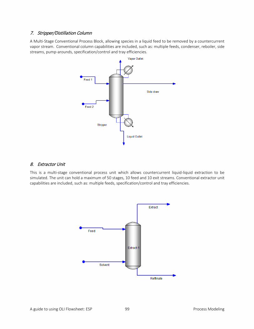
A guide to using OLI Flowsheet: ESP 99 Process Modeling
7. Stripper/Distillation Column
A Multi-Stage Conventional Process Block, allowing species in a liquid feed to be removed by a countercurrent vapor stream. Conventional column capabilities are included, such as: multiple feeds, condenser, reboiler, side streams, pump-arounds, specification/control and tray efficiencies.
8. Extractor Unit
This is a multi-stage conventional process unit which allows countercurrent liquid-liquid extraction to be simulated. The unit can hold a maximum of 50 stages, 10 feed and 10 exit streams. Conventional extractor unit capabilities are included, such as: multiple feeds, specification/control and tray efficiencies.
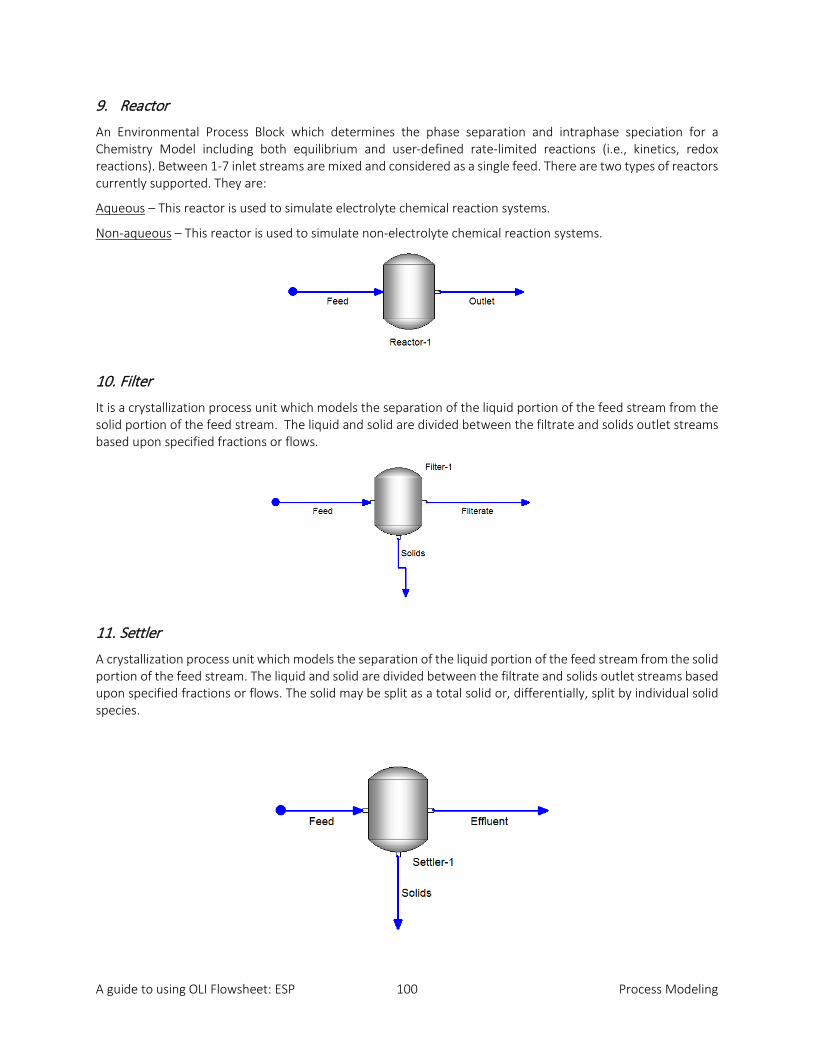
A guide to using OLI Flowsheet: ESP 100 Process Modeling
9. Reactor
An Environmental Process Block which determines the phase separation and intraphase speciation for a Chemistry Model including both equilibrium and user-defined rate-limited reactions (i.e., kinetics, redox reactions). Between 1-7 inlet streams are mixed and considered as a single feed. There are two types of reactors currently supported. They are:
Aqueous – This reactor is used to simulate electrolyte chemical reaction systems.
Non-aqueous – This reactor is used to simulate non-electrolyte chemical reaction systems.
10. Filter
It is a crystallization process unit which models the separation of the liquid portion of the feed stream from the solid portion of the feed stream. The liquid and solid are divided between the filtrate and solids outlet streams based upon specified fractions or flows.
11. Settler
A crystallization process unit which models the separation of the liquid portion of the feed stream from the solid portion of the feed stream. The liquid and solid are divided between the filtrate and solids outlet streams based upon specified fractions or flows. The solid may be split as a total solid or, differentially, split by individual solid species.
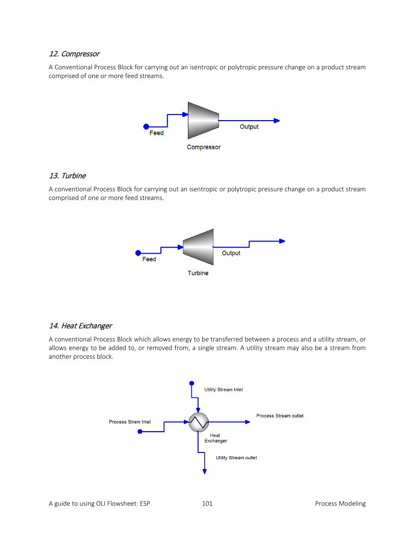
A guide to using OLI Flowsheet: ESP 101 Process Modeling
12. Compressor
A Conventional Process Block for carrying out an isentropic or polytropic pressure change on a product stream comprised of one or more feed streams.
13. Turbine
A conventional Process Block for carrying out an isentropic or polytropic pressure change on a product stream comprised of one or more feed streams.
14. Heat Exchanger
A conventional Process Block which allows energy to be transferred between a process and a utility stream, or allows energy to be added to, or removed from, a single stream. A utility stream may also be a stream from another process block.
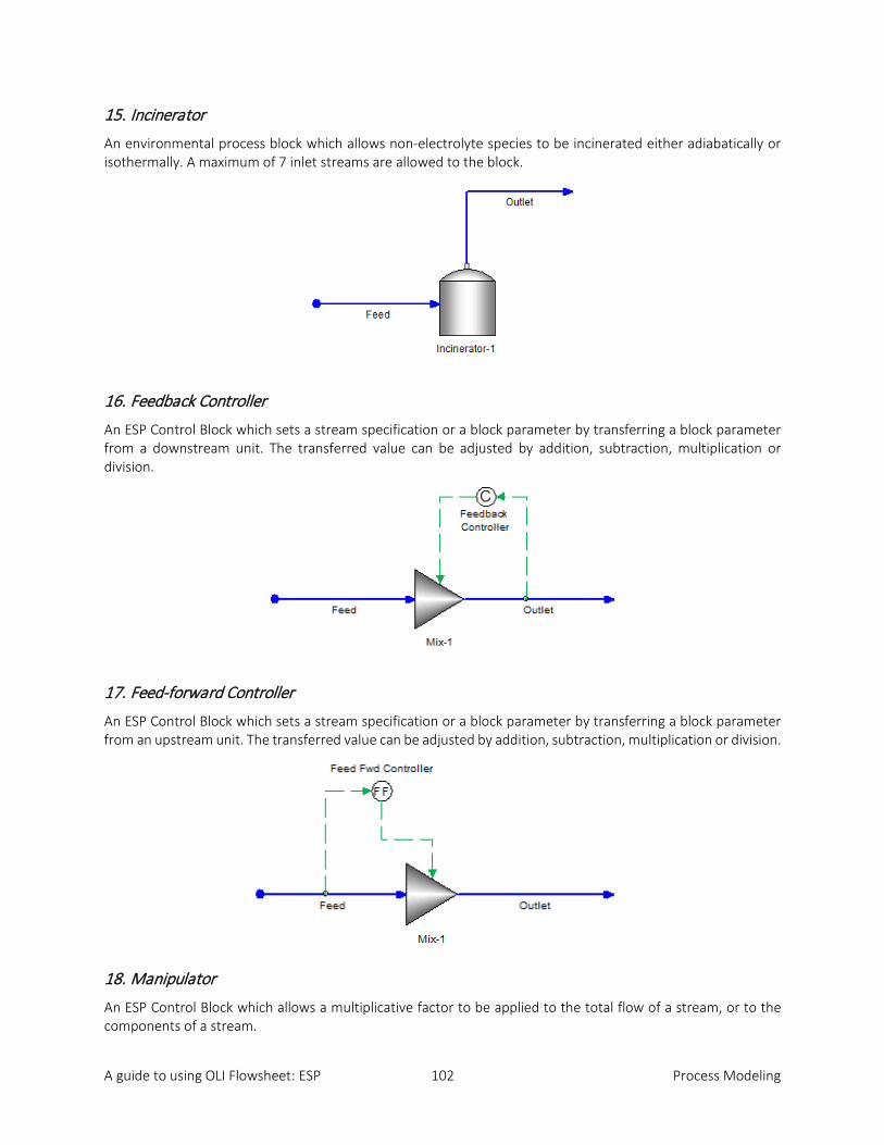
A guide to using OLI Flowsheet: ESP 102 Process Modeling
15. Incinerator
An environmental process block which allows non-electrolyte species to be incinerated either adiabatically or isothermally. A maximum of 7 inlet streams are allowed to the block.
16. Feedback Controller
An ESP Control Block which sets a stream specification or a block parameter by transferring a block parameter from a downstream unit. The transferred value can be adjusted by addition, subtraction, multiplication or division.
17. Feed-forward Controller
An ESP Control Block which sets a stream specification or a block parameter by transferring a block parameter from an upstream unit. The transferred value can be adjusted by addition, subtraction, multiplication or division.
18. Manipulator
An ESP Control Block which allows a multiplicative factor to be applied to the total flow of a stream, or to the components of a stream.
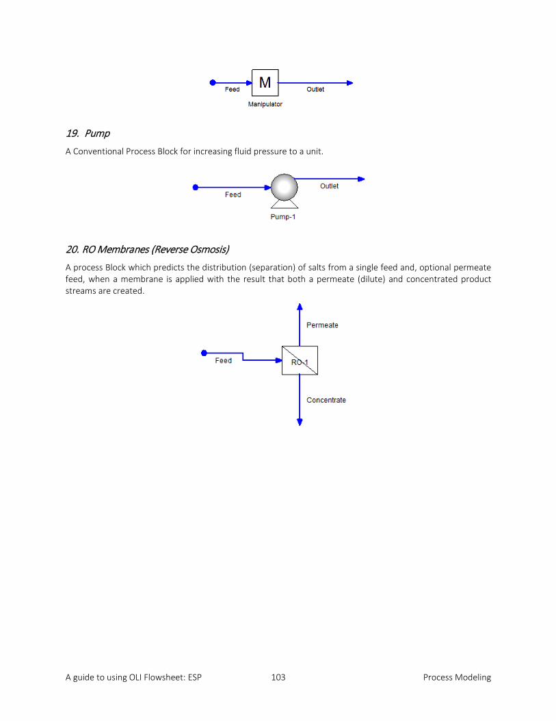
A guide to using OLI Flowsheet: ESP 103 Process Modeling
19. Pump
A Conventional Process Block for increasing fluid pressure to a unit.
20. RO Membranes (Reverse Osmosis)
A process Block which predicts the distribution (separation) of salts from a single feed and, optional permeate feed, when a membrane is applied with the result that both a permeate (dilute) and concentrated product streams are created.
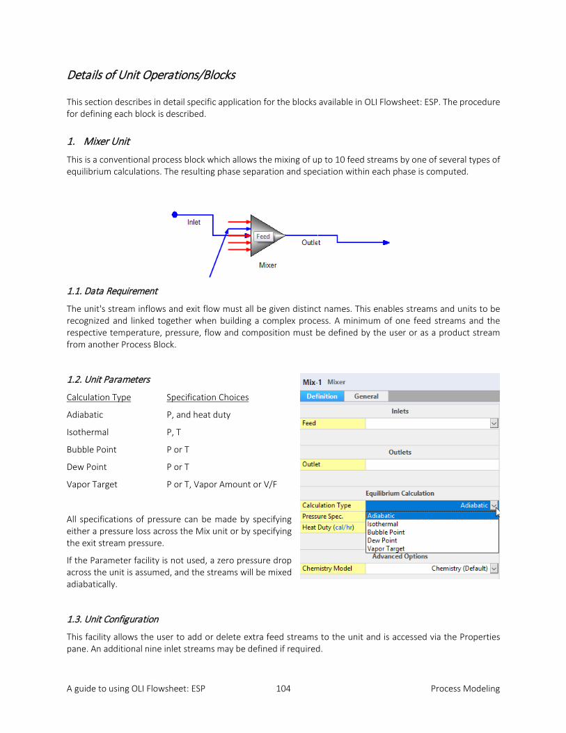
A guide to using OLI Flowsheet: ESP 104 Process Modeling
Details of Unit Operations/Blocks
This section describes in detail specific application for the blocks available in OLI Flowsheet: ESP. The procedure for defining each block is described.
1. Mixer Unit
This is a conventional process block which allows the mixing of up to 10 feed streams by one of several types of equilibrium calculations. The resulting phase separation and speciation within each phase is computed.
1.1. Data Requirement
The unit's stream inflows and exit flow must all be given distinct names. This enables streams and units to be recognized and linked together when building a complex process. A minimum of one feed streams and the respective temperature, pressure, flow and composition must be defined by the user or as a product stream from another Process Block.
1.2. Unit Parameters
Calculation Type Specification Choices
Adiabatic P, and heat duty
Isothermal P, T
Bubble Point P or T
Dew Point P or T
Vapor Target P or T, Vapor Amount or V/F
All specifications of pressure can be made by specifying either a pressure loss across the Mix unit or by specifying the exit stream pressure.
If the Parameter facility is not used, a zero pressure drop across the unit is assumed, and the streams will be mixed adiabatically.
1.3. Unit Configuration
This facility allows the user to add or delete extra feed streams to the unit and is accessed via the Properties pane. An additional nine inlet streams may be defined if required.

A guide to using OLI Flowsheet: ESP 105 Process Modeling
1.4. Guidelines
When additional streams are to be added to the unit, the user must first insure the minimum data requirements for the unit are specified prior to adding the streams.
2. Separator Unit
This is a process unit which allows up to 10 inlet streams to be separated into distinct physical phases. Outlet conditions including suspended solids, entrained liquid, dissolved vapor and dissolved liquid concentrations can be calculated.
1.5. Data Requirements
A minimum of one feed and an aqueous exit stream must be defined. The feed stream must be defined by the user or be a product stream from another Process Block. Both streams must be named, and the inlet temperature, pressure, flow and composition must be specified.
1.6. Units Parameters
Different Equilibrium Calculations are available:
2. Adiabatic 3. Isothermal 4. Bubble point 5. Dew Point 6. Vapor target
Concentration limits can be defined for phase distribution among the outlet streams and is achieved via the Entrainment option under Equilibrium Calculation section.

A guide to using OLI Flowsheet: ESP 106 Process Modeling
These phase distributions include:
* The liquid outlet is the combined aqueous and organic outlet streams.
When the specified limits are exceeded for a particular phase distribution, the surplus quantity remains in its respective phase outlet stream.
Conversely, when one specified phase distribution requires all of the phase, the specification is satisfied, and that phase is eliminated. For example, if the amount specified for the dissolved vapor in the liquid is greater than the amount of vapor present, then all of the vapor is put in the liquid outlet, and the vapor outlet is set to zero.
If two specified phase distributions cannot be met, the error condition is raised.
1.3. Unit Configuration This facility allows the user to add or delete extra inlet streams to the unit and is accessed via the Properties Pane. An additional nine feeds may be defined if required. 1.4. Guidelines When additional streams are to be added to the unit the user must first insure the minimum data requirements for the unit are specified prior to adding new inlet streams. 3. Neutralizer Unit This is an environmental process block which allows up to 10 feed streams to be neutralized by the addition of a suitable reagent. The neutralization can be modeled adiabatically by mixing the inlet streams, by varying the neutralizing reagent flow to meet a fixed pH set point.
Distribution Stream
Suspended solids Liquid* outlet stream Entrained liquid concentration Vapor outlet stream Dissolved liquid Solid outlet stream Dissolved vapor Liquid* outlet stream Dissolved aqueous phase Organic outlet stream Dissolved organic phase Aqueous outlet stream
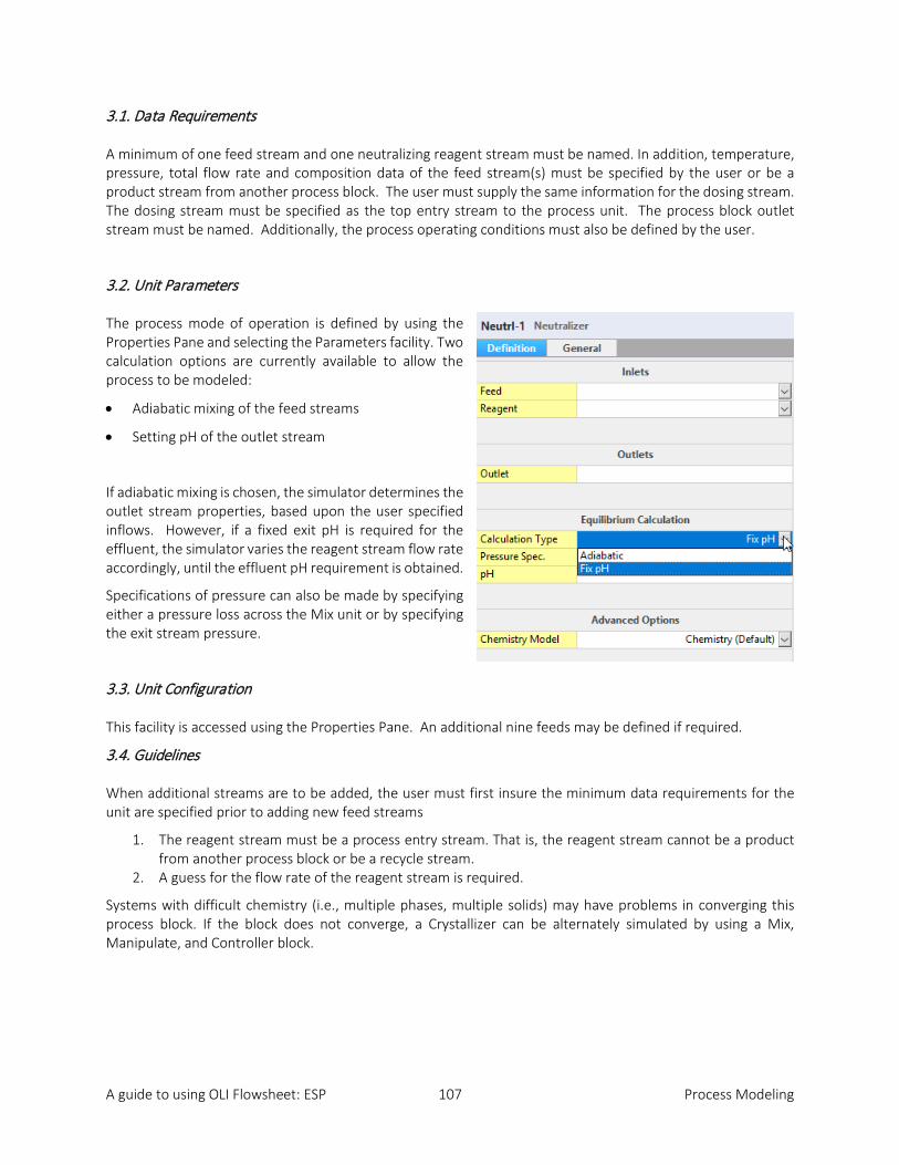
A guide to using OLI Flowsheet: ESP 107 Process Modeling
3.1. Data Requirements
A minimum of one feed stream and one neutralizing reagent stream must be named. In addition, temperature, pressure, total flow rate and composition data of the feed stream(s) must be specified by the user or be a product stream from another process block. The user must supply the same information for the dosing stream. The dosing stream must be specified as the top entry stream to the process unit. The process block outlet stream must be named. Additionally, the process operating conditions must also be defined by the user.
3.2. Unit Parameters
The process mode of operation is defined by using the Properties Pane and selecting the Parameters facility. Two calculation options are currently available to allow the process to be modeled:
• Adiabatic mixing of the feed streams
• Setting pH of the outlet stream
If adiabatic mixing is chosen, the simulator determines the outlet stream properties, based upon the user specified inflows. However, if a fixed exit pH is required for the effluent, the simulator varies the reagent stream flow rate accordingly, until the effluent pH requirement is obtained.
Specifications of pressure can also be made by specifying either a pressure loss across the Mix unit or by specifying the exit stream pressure.
3.3. Unit Configuration
This facility is accessed using the Properties Pane. An additional nine feeds may be defined if required.
3.4. Guidelines
When additional streams are to be added, the user must first insure the minimum data requirements for the unit are specified prior to adding new feed streams
1. The reagent stream must be a process entry stream. That is, the reagent stream cannot be a product from another process block or be a recycle stream.
2. A guess for the flow rate of the reagent stream is required.
Systems with difficult chemistry (i.e., multiple phases, multiple solids) may have problems in converging this process block. If the block does not converge, a Crystallizer can be alternately simulated by using a Mix, Manipulate, and Controller block.

A guide to using OLI Flowsheet: ESP 108 Process Modeling
4. Splitter Unit
4.1. Flow Split Unit
This is a conventional process unit which allows a single inlet to be divided into a maximum of 7 outlet streams, all with the same temperature, pressure and relative species content.
4.1.1. Data Requirement
The unit's stream inflow and exit flows must all be given distinct names, so that they can be linked to other process units, if required.
One feed stream, and a minimum of two exit streams must be defined by the user. The inlet stream temperature, pressure, flow and composition data must be defined or be a product stream from another Process Block. Additionally, the split outlet stream fractions or flows must be defined.
4.1.2. Unit Parameters
The stream outlet fractions are defined using the Action Key and then by selecting the Parameters facility. The outlet fractions may be defined on one of a variety of bases, (e.g., mole fractions, flow, etc.) which are then automatically normalized by the software such that the sum of the outlet fractions is equal to 1.
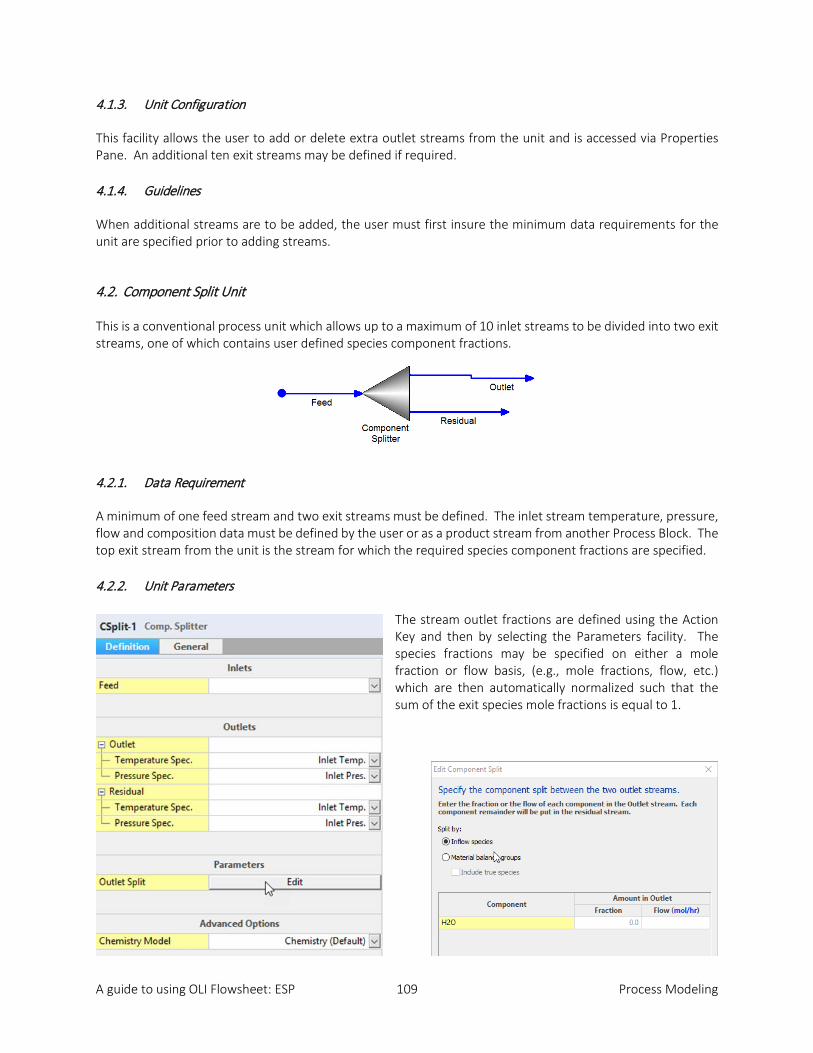
A guide to using OLI Flowsheet: ESP 109 Process Modeling
4.1.3. Unit Configuration
This facility allows the user to add or delete extra outlet streams from the unit and is accessed via Properties Pane. An additional ten exit streams may be defined if required.
4.1.4. Guidelines
When additional streams are to be added, the user must first insure the minimum data requirements for the unit are specified prior to adding streams.
4.2. Component Split Unit
This is a conventional process unit which allows up to a maximum of 10 inlet streams to be divided into two exit streams, one of which contains user defined species component fractions.
4.2.1. Data Requirement
A minimum of one feed stream and two exit streams must be defined. The inlet stream temperature, pressure, flow and composition data must be defined by the user or as a product stream from another Process Block. The top exit stream from the unit is the stream for which the required species component fractions are specified.
4.2.2. Unit Parameters
The stream outlet fractions are defined using the Action Key and then by selecting the Parameters facility. The species fractions may be specified on either a mole fraction or flow basis, (e.g., mole fractions, flow, etc.) which are then automatically normalized such that the sum of the exit species mole fractions is equal to 1.

A guide to using OLI Flowsheet: ESP 110 Process Modeling
4.2.3. Unit Configuration
This facility allows the user to add or delete extra inlet streams to the unit and is accessed via the Properties Pane. An additional six feeds may be defined if required.
4.4.4. Guidelines
When additional streams are to be added, the user must first insure the minimum data requirements for the unit are specified prior to adding new streams.
5. Absorber Unit
This is a multi-stage conventional or environmental process unit which allows species in a vapor feed to be absorbed by a countercurrent liquid stream. The unit can hold up to a maximum of 50 stages and up to a maximum of 10 feed and 10 product streams.
When this block is selected the user can choose either an electrolyte column or a non-electrolyte column (if a non-electrolyte model was created). In the case of an electrolyte column, an aqueous phase must be present in every liquid stream. The liquid feed and/or liquid product can contain both an aqueous and non-aqueous liquid phase or just an aqueous phase alone. In the case of a non-electrolyte column, there is only the non-electrolyte liquid phase (electrolyte chemistry is not considered).
5.1. Data Requirement
A minimum of one liquid stream entering the top of the column and one vapor stream entering the bottom of the unit must be specified. The respective feed stream temperature, pressure, flow and composition must be defined by the user or be a product stream from another Process Block.
When defining the feed stream, the temperature and pressures of each stream should be such that the species components reside in the correct phase for the respective stream.
The column exit vapor and liquid streams must be named, in addition to various column parameters.

A guide to using OLI Flowsheet: ESP 111 Process Modeling
5.2. Column Configuration
Column parameters can be defined, via the Properties Pane. Seven options are available:
• Calculation Method: − Equilibrium − Mass transfer Ltd.
• Number of Stages: The default number is 10 stages.
• Include condenser/reboiler: This option allows the
user to delete, or insert, these respective units from/to the column. Initially, the process block does not include the two heat exchanger units.
• Inlets: This function is optional and allows the user to specify up to 8 additional feed streams to the column.
• Outlets: This function is optional and allows the user to specify up to 8 additional product streams from the column.
• Pumparounds: This function is optional and allows the
user to specify side stream pumparounds if required. Pumparounds must be from a lower to a higher stage of the column and the flow rate must be defined.
5.3. Column Parameters
The column operating parameters are accessed using Properties Pane. Eight options are available:
• Spec/Controls: This function is optional and allows the user to manipulate parameters (e.g., heat exchange duty) to meet specifications in the column operation. For example, vapor and/or liquid composition specifications, stage operating temperature and vapor and/or liquid stream component flow rate specifications can all be achieved.
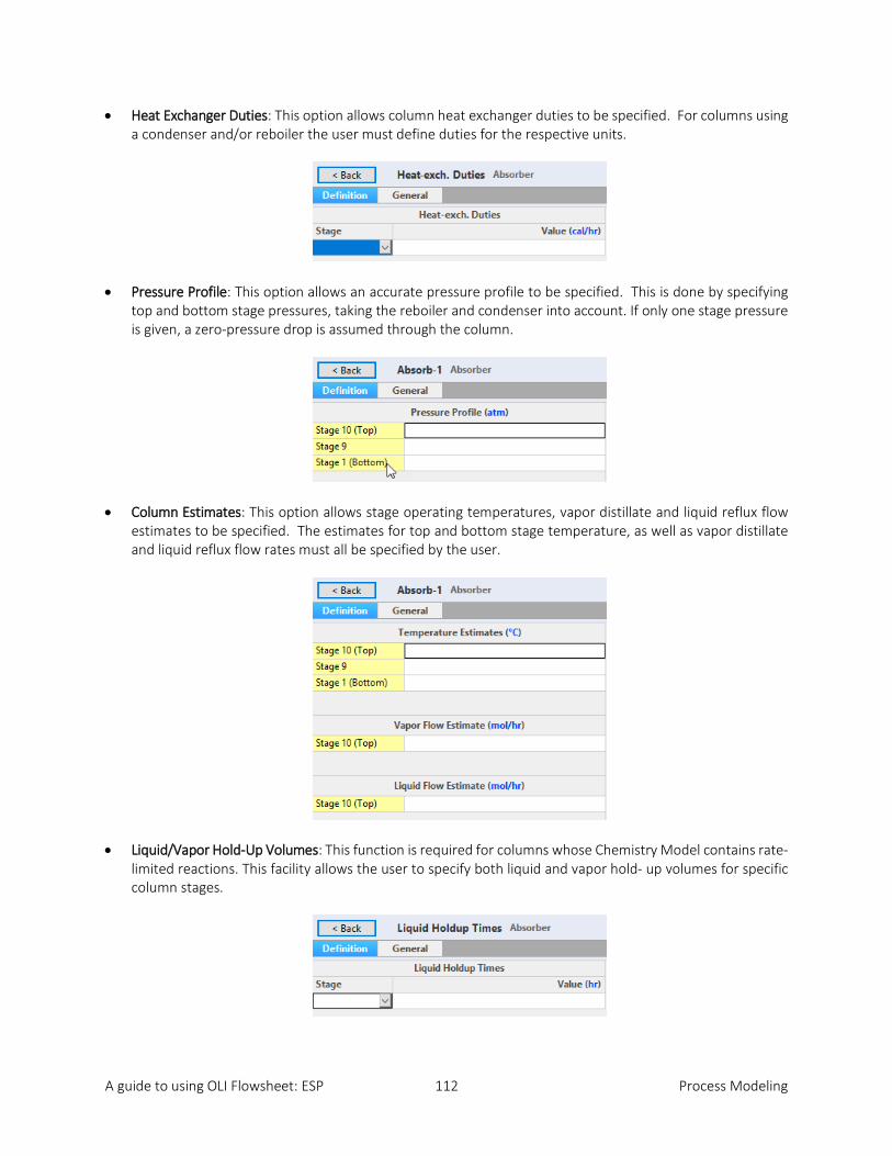
A guide to using OLI Flowsheet: ESP 112 Process Modeling
• Heat Exchanger Duties: This option allows column heat exchanger duties to be specified. For columns using a condenser and/or reboiler the user must define duties for the respective units.
• Pressure Profile: This option allows an accurate pressure profile to be specified. This is done by specifying top and bottom stage pressures, taking the reboiler and condenser into account. If only one stage pressure is given, a zero-pressure drop is assumed through the column.
• Column Estimates: This option allows stage operating temperatures, vapor distillate and liquid reflux flow estimates to be specified. The estimates for top and bottom stage temperature, as well as vapor distillate and liquid reflux flow rates must all be specified by the user.
• Liquid/Vapor Hold-Up Volumes: This function is required for columns whose Chemistry Model contains rate-limited reactions. This facility allows the user to specify both liquid and vapor hold- up volumes for specific column stages.

A guide to using OLI Flowsheet: ESP 113 Process Modeling
• Tray Efficiencies: This function is enabled when the calculation method chosen is Equilibrium. This function is optional and allows the user to specify Murphree efficiencies for the column stages. If no data is entered the stage efficiency is assumed to be 1.0.
• Mass Transfer: This function is enabled when the
calculation method chosen is the Mass transfer Ltd. This option allows the user to specify vapor-liquid mass and heat transfer coefficients on each stage of the column. The coefficients are overall coefficients and apply to all components. The interfacial transfer area must also be specified. If the same coefficients are used throughout the column, the coefficient may be varied to meet a composition specification by means of the spec/control parameters.
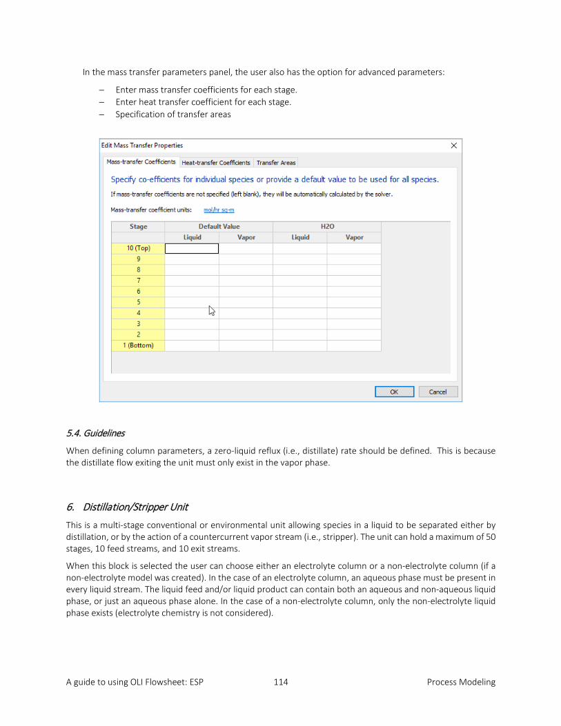
A guide to using OLI Flowsheet: ESP 114 Process Modeling
In the mass transfer parameters panel, the user also has the option for advanced parameters:
− Enter mass transfer coefficients for each stage. − Enter heat transfer coefficient for each stage. − Specification of transfer areas
5.4. Guidelines
When defining column parameters, a zero-liquid reflux (i.e., distillate) rate should be defined. This is because the distillate flow exiting the unit must only exist in the vapor phase.
6. Distillation/Stripper Unit
This is a multi-stage conventional or environmental unit allowing species in a liquid to be separated either by distillation, or by the action of a countercurrent vapor stream (i.e., stripper). The unit can hold a maximum of 50 stages, 10 feed streams, and 10 exit streams.
When this block is selected the user can choose either an electrolyte column or a non-electrolyte column (if a non-electrolyte model was created). In the case of an electrolyte column, an aqueous phase must be present in every liquid stream. The liquid feed and/or liquid product can contain both an aqueous and non-aqueous liquid phase, or just an aqueous phase alone. In the case of a non-electrolyte column, only the non-electrolyte liquid phase exists (electrolyte chemistry is not considered).

A guide to using OLI Flowsheet: ESP 115 Process Modeling
6.1. Data Requirement
A minimum of one feed stream and two exit streams (i.e., distillate and bottoms) must be named when using the unit for distillation. An additional feed must be added when using the unit as a stripper. The feed stream temperature, pressure, flow and composition data must be specified by the user or be a product stream from another Process Block. The number of stages will default to 10 and appear that way on the initial screen. The user may override this value. If there is a condenser or reboiler, these will count as stages. Additionally, various column operating parameter information must be supplied by the user.
6.2. Column Configuration
Additional column parameters can be defined, via configuration pane. Seven options are available:
• Calculation Method: − Equilibrium − Mass transfer Ltd.
• Number of Stages: The default number is 10 stages.
• Include condenser/reboiler: This option allows the user to
delete, or insert, these respective units from/to the column. Initially, the process block includes the two units on the display.
• Inlets: This function is optional and allows the user to specify up to 8 additional feed streams to the column.
• Outlets: This function is optional and allows the user to specify up to 8 additional product streams from the column.
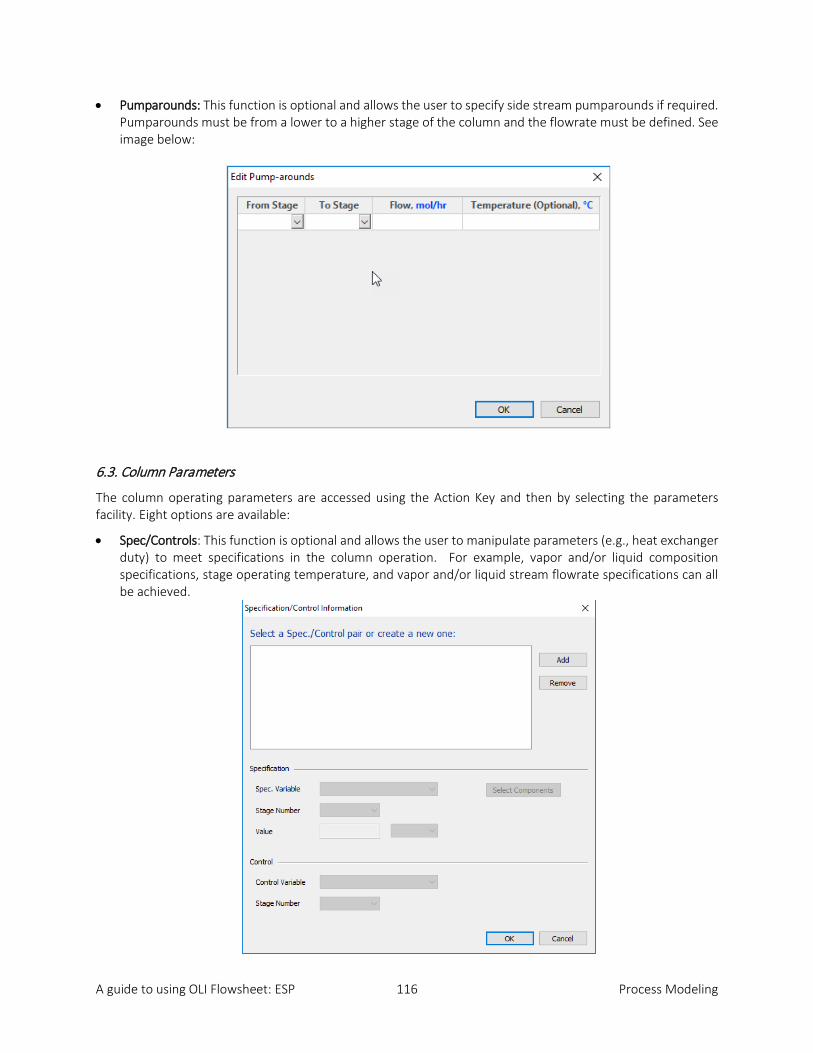
A guide to using OLI Flowsheet: ESP 116 Process Modeling
• Pumparounds: This function is optional and allows the user to specify side stream pumparounds if required. Pumparounds must be from a lower to a higher stage of the column and the flowrate must be defined. See image below:
6.3. Column Parameters
The column operating parameters are accessed using the Action Key and then by selecting the parameters facility. Eight options are available:
• Spec/Controls: This function is optional and allows the user to manipulate parameters (e.g., heat exchanger duty) to meet specifications in the column operation. For example, vapor and/or liquid composition specifications, stage operating temperature, and vapor and/or liquid stream flowrate specifications can all be achieved.

A guide to using OLI Flowsheet: ESP 117 Process Modeling
• Heat Exchanger Duties: This option allows column and pumparound heat exchanger duties to be specified. For columns using a condenser and/or reboiler, the user must define duties for the respective units. Negative heat duties imply heat removal.
• Pressure Profile: This option allows an accurate pressure profile to be specified. This is done by specifying top and bottom stage pressures, taking the reboiler and condenser into account. If only one stage pressure is given, a zero pressure drop through the column is assumed. If no values are given, the entire column is assumed to operate at atmospheric pressure.
• Estimates: This option allows stage operating temperatures, vapor distillate and liquid reflux flow estimates to be specified. The estimates for top and bottom stage temperature, as well as the vapor distillate rate and liquid reflux flowrates, must all be specified by the user.
• Liquid/Vapor Hold-Up Volumes: This function is required for columns whose chemistry contains rate-limited reactions. This facility allows the user to specify both liquid and vapor hold-up volumes for specific column stages.
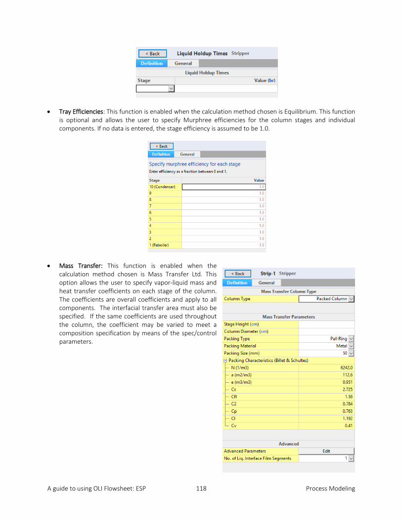
A guide to using OLI Flowsheet: ESP 118 Process Modeling
• Tray Efficiencies: This function is enabled when the calculation method chosen is Equilibrium. This function is optional and allows the user to specify Murphree efficiencies for the column stages and individual components. If no data is entered, the stage efficiency is assumed to be 1.0.
• Mass Transfer: This function is enabled when the calculation method chosen is Mass Transfer Ltd. This option allows the user to specify vapor-liquid mass and heat transfer coefficients on each stage of the column. The coefficients are overall coefficients and apply to all components. The interfacial transfer area must also be specified. If the same coefficients are used throughout the column, the coefficient may be varied to meet a composition specification by means of the spec/control parameters.

A guide to using OLI Flowsheet: ESP 119 Process Modeling
In the mass transfer parameters panel, the user also has the option for advanced parameters:
− Enter mass transfer coefficients for each stage. − Enter heat transfer coefficient for each stage. − Specification of transfer areas
• Condenser: This function is optional and allows the user to specify the type of condenser. If no data is entered, the condenser is assumed to be partial condenser. Four types of condensers can be selected:
− Partial condenser − Total condenser − Sub-cooled Total condenser − Decanter
6.4. Guidelines
1. For columns with condenser and/or reboiler units the heat duty estimates defined by the user must be such that a vapor flow exists on the bottom stage and a liquid phase flow exists on the top stage of the column respectively.

A guide to using OLI Flowsheet: ESP 120 Process Modeling
2. The column can only operate if two (or optionally three) phases exist on every stage of the column.
3. For columns without a condenser and/or reboiler unit, a feed stream must be specified entering at the respective position of the omitted unit. The phase of this stream must be correctly defined. A liquid phase feed stream is required as an alternative to a column condenser, and a vapor phase stream in place of a reboiler unit (i.e., the column must have two phases flowing to and from every stage).
4. When defining a stripper unit, an all liquid feed stream must be specified entering the top of the column
and the stripping vapor must enter the bottom of the unit.
5. When defining stripper column parameters, a zero-liquid reflux (i.e., distillate) flow must be made. This is because the distillate flow exiting the unit must only exist in the vapor phase.
6. All column stages are numbered from bottom to top.
7. If a feed stream contains both a vapor and a liquid phase, the liquid goes to the feed tray specified by the
user and the vapor goes to the stage above.
7. Extractor Unit
7.1. Data Requirement
A minimum of one aqueous feed stream must be defined entering the top of the column, and the solvent stream entering the bottom of the unit. The respective feed streams temperatures, pressures, flows and compositions must be specified, or be a product stream from another Process Block, and the unit outflows named. Additionally, various column operating parameter information must be specified by the user.
7.2. Column Configuration
Additional column parameters can be defined, via the Action Key and selecting the Config facility. Five options are available:
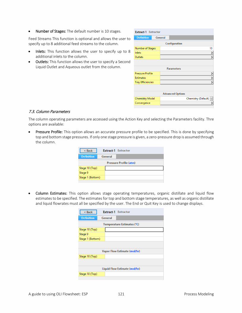
A guide to using OLI Flowsheet: ESP 121 Process Modeling
• Number of Stages: The default number is 10 stages.
Feed Streams This function is optional and allows the user to specify up to 8 additional feed streams to the column.
• Inlets: This function allows the user to specify up to 8 additional inlets to the column.
• Outlets: This function allows the user to specify a Second Liquid Outlet and Aqueous outlet from the column.
7.3. Column Parameters
The column operating parameters are accessed using the Action Key and selecting the Parameters facility. Thre options are available:
• Pressure Profile: This option allows an accurate pressure profile to be specified. This is done by specifying top and bottom stage pressures. If only one stage pressure is given, a zero-pressure drop is assumed through the column.
• Column Estimates: This option allows stage operating temperatures, organic distillate and liquid flow estimates to be specified. The estimates for top and bottom stage temperatures, as well as organic distillate and liquid flowrates must all be specified by the user. The End or Quit Key is used to change displays.
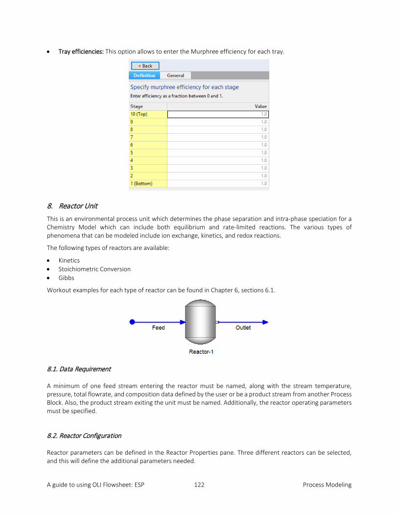
A guide to using OLI Flowsheet: ESP 122 Process Modeling
• Tray efficiencies: This option allows to enter the Murphree efficiency for each tray.
8. Reactor Unit
This is an environmental process unit which determines the phase separation and intra-phase speciation for a Chemistry Model which can include both equilibrium and rate-limited reactions. The various types of phenomena that can be modeled include ion exchange, kinetics, and redox reactions.
The following types of reactors are available:
• Kinetics • Stoichiometric Conversion • Gibbs
Workout examples for each type of reactor can be found in Chapter 6, sections 6.1.
8.1. Data Requirement
A minimum of one feed stream entering the reactor must be named, along with the stream temperature, pressure, total flowrate, and composition data defined by the user or be a product stream from another Process Block. Also, the product stream exiting the unit must be named. Additionally, the reactor operating parameters must be specified.
8.2. Reactor Configuration
Reactor parameters can be defined in the Reactor Properties pane. Three different reactors can be selected, and this will define the additional parameters needed.

A guide to using OLI Flowsheet: ESP 123 Process Modeling
8.2.1. Kinetics Reactor
The chemical kinetics of the reaction are described by the Arrhenius Equation which is specified in the Chemistry Model.
8.2.1.1. Reactor Properties
For the Kinetics reactor you can specify kinetics parameters.

A guide to using OLI Flowsheet: ESP 124 Process Modeling
8.2.1.2. Equilibrium Calculations
Several options are given in this panel:
• Calculation Type: Can be Adiabatic or Isothermal • Pressure Spec.: Can be Min. inlet pressure, absolute pressure, and pressure drop. • Pressure Drop: Specify the pressure drop within the block. • Temperature: If the calculation is isothermal • Heat duty: If the calculation is adiabatic
8.2.2. Stoichiometric Conversion Reactor
Stoichiometric reactors use a simple stoichiometric relationship between reactants and products. There is no time factor for these reactions.
8.2.2.1. Reactor Properties
For the Conversion Reactor you can specify Reactions.
8.2.2.2. Equilibrium Calculations
Several options are given in this panel:
• Calculation Type: Can be Adiabatic or Isothermal • Pressure Spec.: Can be Min. inlet pressure, absolute pressure, and pressure drop.
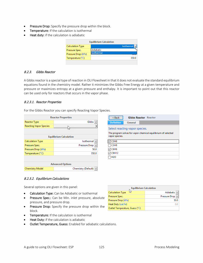
A guide to using OLI Flowsheet: ESP 125 Process Modeling
• Pressure Drop: Specify the pressure drop within the block. • Temperature: If the calculation is isothermal • Heat duty: if the calculation is adiabatic
8.2.3. Gibbs Reactor
A Gibbs reactor is a special type of reaction in OLI Flowsheet in that it does not evaluate the standard equilibrium equations found in the chemistry model. Rather it minimizes the Gibbs Free Energy at a given temperature and pressure or maximizes entropy at a given pressure and enthalpy. It is important to point out that this reactor can be used only for reactors that occurs in the vapor phase.
8.2.3.1. Reactor Properties
For the Gibbs Reactor you can specify Reacting Vapor Species.
8.2.3.2. Equilibrium Calculations
Several options are given in this panel:
• Calculation Type: Can be Adiabatic or Isothermal • Pressure Spec.: Can be Min. inlet pressure, absolute
pressure, and pressure drop. • Pressure Drop: Specify the pressure drop within the
block. • Temperature: If the calculation is isothermal • Heat Duty: if the calculation is adiabatic • Outlet Temperature, Guess: Enabled for adiabatic calculations.

A guide to using OLI Flowsheet: ESP 126 Process Modeling
9. Filter Unit
This is a crystallization process unit which models the separation of the liquid portion of the feed stream from the solid portion of the feed stream. The liquid and solid are divided between the filtrate and solids outlet streams based upon specified fractions or flows.
9.1. Data Requirement
One feed stream entering the Filter must be named, along with the stream temperature, pressure, total flowrate, and composition data defined by the user or be a product stream from another Process Block. Also, the outlet (filtrate and solids) streams exiting the unit must be named. The filter operating parameters must be specified.
9.2. Unit Parameters
The Filter operating conditions are specified using the Edit button.
Two basic conditions must be specified:
1. Split of the total liquid to the filtrate and solids streams, and 2. Split of the solid between the filtrate and solids streams.
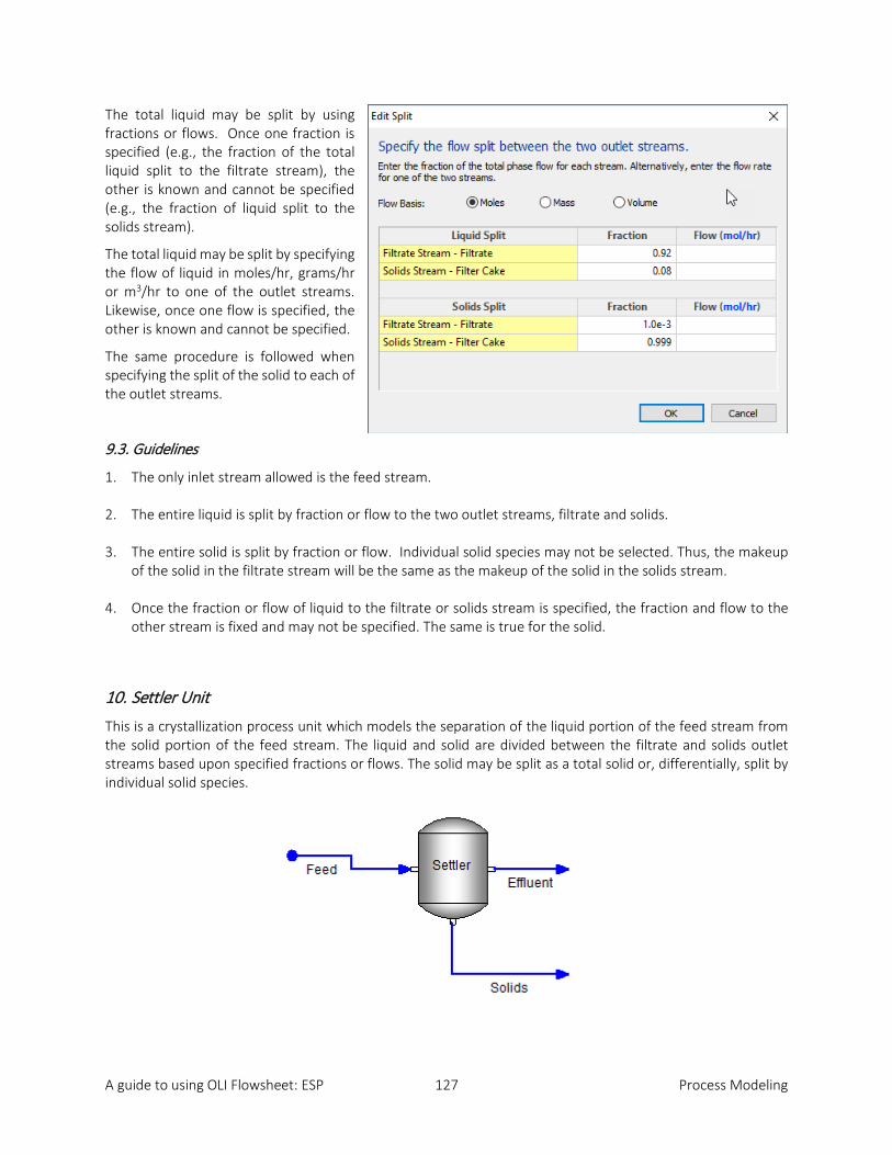
A guide to using OLI Flowsheet: ESP 127 Process Modeling
The total liquid may be split by using fractions or flows. Once one fraction is specified (e.g., the fraction of the total liquid split to the filtrate stream), the other is known and cannot be specified (e.g., the fraction of liquid split to the solids stream).
The total liquid may be split by specifying the flow of liquid in moles/hr, grams/hr or m3/hr to one of the outlet streams. Likewise, once one flow is specified, the other is known and cannot be specified.
The same procedure is followed when specifying the split of the solid to each of the outlet streams.
9.3. Guidelines
1. The only inlet stream allowed is the feed stream.
2. The entire liquid is split by fraction or flow to the two outlet streams, filtrate and solids.
3. The entire solid is split by fraction or flow. Individual solid species may not be selected. Thus, the makeup of the solid in the filtrate stream will be the same as the makeup of the solid in the solids stream.
4. Once the fraction or flow of liquid to the filtrate or solids stream is specified, the fraction and flow to the
other stream is fixed and may not be specified. The same is true for the solid.
10. Settler Unit
This is a crystallization process unit which models the separation of the liquid portion of the feed stream from the solid portion of the feed stream. The liquid and solid are divided between the filtrate and solids outlet streams based upon specified fractions or flows. The solid may be split as a total solid or, differentially, split by individual solid species.

A guide to using OLI Flowsheet: ESP 128 Process Modeling
10.1. Data Requirement
One feed stream entering the Settler must be named, along with the stream temperature, pressure, total flowrate, and composition data defined by the user or be a product stream from another Process Block. Also, the outlet (filtrate and solids) streams exiting the unit must be named. Additionally, the Settler operating parameters must be specified.
10.2. Unit Parameters
The Filter operating conditions are specified using the Edit Button.
Two basic conditions must be specified:
1. split of the total liquid to the filtrate and solids streams, and 2. split of the solid, or individual solid species, between the filtrate and solids streams.
The total liquid may be split by using fractions or flows. Once one fraction is specified (e.g., the fraction of the total liquid split to the filtrate stream), the other is known and cannot be specified (e.g., the fraction of liquid split to the solids stream). The total liquid may be split by specifying the flow of liquid in moles/hr, grams/hr or m3/hr to one of the outlet streams. Likewise, once one flow is specified, the other is known and cannot be specified.
The Settler also offers the option to split specific solids from a solid stream.
The total solid may be split by using fractions or flows or the solid may be split by specifying the fraction or flow of specific solid species to each of the outlet streams. A combination of the two may also be used. That is, you may split one or more individual solid species by fraction or flow and then split the remainder of the solid by an overall fraction or flow. Since the solid may be split by individual solid species, the resulting solid portion of each of the outlet streams are not necessarily of the same makeup.

A guide to using OLI Flowsheet: ESP 129 Process Modeling
10.3. Guidelines
1. The only inlet stream allowed is the feed stream.
2. The entire liquid is split by fraction or flow to the two outlet streams, filtrate and solids.
3. When splitting the solid, individual solid species may be selected. Any solid species not selected will be split using the overall solid split fraction or flow. Thus, the makeup of the solid in the filtrate stream will be the same as the makeup of the solid in the solids stream.
4. Once the fraction or flow of liquid to the filtrate or solids stream is specified, the fraction and flow to the
other stream is fixed and may not be specified. The same is true for the solid.
11. Compressor Unit
This is a conventional process block which allows the compression of 1-7 feed streams into a single product stream. The compression can be carried out on either an isentropic or polytropic basis. The resulting phase separation and speciation within each phase is computed.

A guide to using OLI Flowsheet: ESP 130 Process Modeling
11.1. Data Requirement
The unit’s stream inflows and exit flow must be given distinct names. This enables streams and units to be recognized and linked together when building a complex process. A minimum of one feed stream, together with its conditions must be defined by the user or said stream must be a product stream from another process block.
11.2. Unit Parameters
The parameters available to define the compressor are as follows:
Parameter Value Comment
Compressor Isentropic or polytropic Must provide
Outlet Pressure User Must provide
Isentropic Efficiency User (0.0 to 1.0) Default = 0.72
Polytropic Efficiency User (0.0 to 1.0) Default = 0.72
Mechanical Efficiency User (0.0 to 1.0) Default = 1.0
11.3. Unit Configuration
This unit allows the user to add or delete extra feed streams. An additional six inlet streams may be defined if required.
11.4. Guidelines
When additional streams are to be added to the unit, the user must first insure the minimum data requirements for the unit are specified prior to adding new streams.
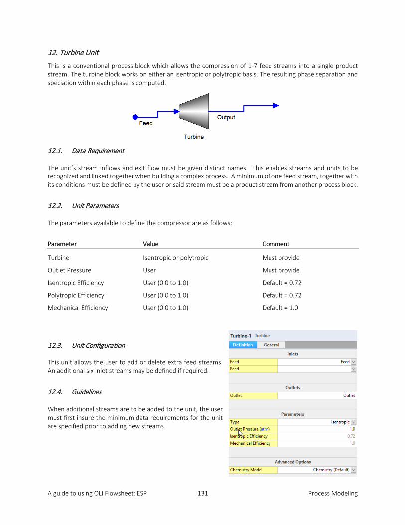
A guide to using OLI Flowsheet: ESP 131 Process Modeling
12. Turbine Unit
This is a conventional process block which allows the compression of 1-7 feed streams into a single product stream. The turbine block works on either an isentropic or polytropic basis. The resulting phase separation and speciation within each phase is computed.
12.1. Data Requirement
The unit’s stream inflows and exit flow must be given distinct names. This enables streams and units to be recognized and linked together when building a complex process. A minimum of one feed stream, together with its conditions must be defined by the user or said stream must be a product stream from another process block.
12.2. Unit Parameters
The parameters available to define the compressor are as follows:
Parameter Value Comment
Turbine Isentropic or polytropic Must provide
Outlet Pressure User Must provide
Isentropic Efficiency User (0.0 to 1.0) Default = 0.72
Polytropic Efficiency User (0.0 to 1.0) Default = 0.72
Mechanical Efficiency User (0.0 to 1.0) Default = 1.0
12.3. Unit Configuration
This unit allows the user to add or delete extra feed streams. An additional six inlet streams may be defined if required.
12.4. Guidelines
When additional streams are to be added to the unit, the user must first insure the minimum data requirements for the unit are specified prior to adding new streams.
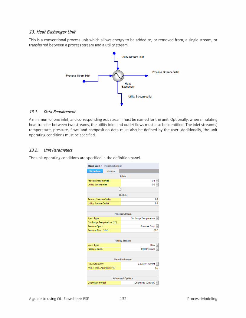
A guide to using OLI Flowsheet: ESP 132 Process Modeling
13. Heat Exchanger Unit
This is a conventional process unit which allows energy to be added to, or removed from, a single stream, or transferred between a process stream and a utility stream.
13.1. Data Requirement
A minimum of one inlet, and corresponding exit stream must be named for the unit. Optionally, when simulating heat transfer between two streams, the utility inlet and outlet flows must also be identified. The inlet stream(s) temperature, pressure, flows and composition data must also be defined by the user. Additionally, the unit operating conditions must be specified.
13.2. Unit Parameters
The unit operating conditions are specified in the definition panel.
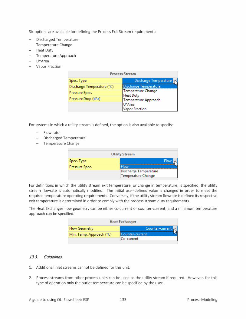
A guide to using OLI Flowsheet: ESP 133 Process Modeling
Six options are available for defining the Process Exit Stream requirements:
− Discharged Temperature − Temperature Change − Heat Duty − Temperature Approach − U*Area − Vapor Fraction
For systems in which a utility stream is defined, the option is also available to specify:
− Flow rate − Discharged Temperature − Temperature Change
For definitions in which the utility stream exit temperature, or change in temperature, is specified, the utility stream flowrate is automatically modified. The initial user-defined value is changed in order to meet the required temperature operating requirements. Conversely, if the utility stream flowrate is defined its respective exit temperature is determined in order to comply with the process stream duty requirements.
The Heat Exchanger flow geometry can be either co-current or counter-current, and a minimum temperature approach can be specified.
13.3. Guidelines
1. Additional inlet streams cannot be defined for this unit.
2. Process streams from other process units can be used as the utility stream if required. However, for this type of operation only the outlet temperature can be specified by the user.

A guide to using OLI Flowsheet: ESP 134 Process Modeling
14. Incinerator
14.1. Data Requirement
A minimum of one feed stream to the unit must be defined, and its temperature, pressure, total flowrate and composition data should be specified by the user or be the product stream from another Process Block. Note that the oxidation vapor stream composition (i.e., the air being used to burn the feed) must also be included as part of the feed stream(s) definition. The waste stream exiting the unit must also be identified.
14.2. Unit Parameters
This unit can operate adiabatically or isothermally, one of which must be selected. For isothermal operation, the incinerator operating temperature must be supplied by the user.
14.3. Unit Configuration
This facility allows the user to add or delete extra inlet streams to the unit. An additional 3 feeds may be defined if required.
14.4. Guidelines
When using this unit, the user must insure a Non-Electrolyte Chemistry Model.
For clarification purposes it is advised that the oxidation vapor stream is specified as a separate inlet flow to the unit, rather than as part of the feed stream composition.
Species that may form through a reduction/oxidation process and be in the product stream must be named as a species in the Chemistry Model (e.g., NOx compounds, SO2, etc.).

A guide to using OLI Flowsheet: ESP 135 Process Modeling
15. Feedback Controller
This is an Control Block which allows the user to specify a particular stream property by adjusting a block parameter of another process block.
15.1. Data Requirement
The Controller definition can be divided into two parts: defining the stream specification and defining the block parameter of the process block to be varied to meet the stream specification.
15.2. Defining the Target Specification
The target stream is chosen from the streams already defined in other process block. Only streams which have been defined can be named in the Controller Block.
The stream's specification type is then selected from a list of possible specification types, which include:
− Temperature − Pressure

A guide to using OLI Flowsheet: ESP 136 Process Modeling
− pH − Flow (When flow is selected as a specification, the phase and the units can be named) − True species composition of the stream (When composition is selected as a specification, the phase and
units of the composition can also be named) − Material Balance Group Composition (The target composition can be named in terms of either the species
in the solution (e.g., CACO3), or in terms of the material balance groups in the solution e.g., Ca (+2), C (+4), or O (-2)).
The Feedback controller basis needs to be specified. It can be either volume, mass or moles.
Different phases can also be specified:
15.3. Defining Control Parameter
The controlling block, which will be varied to meet the stream specification, is selected from a list of process blocks already defined. Once the controlling block is selected, the parameters available for that block are listed.
For example:
Or

A guide to using OLI Flowsheet: ESP 137 Process Modeling
15.4. Unit Parameters
Controller parameters can be set which guide the convergence of the Controlling Block. These optional parameters are accessed via in the Convergence Options.
The parameters which can be set are:
• Step Sized Method: Which are divided into three different methods. One of three calculation step size methods can be selected. The Slope Technique is the default − Slope Technique: The slope
between the last two guesses determines the next guess, unless the step size minimum or maximum is exceeded. This is the fastest technique, provided there are no large differences in slopes (as there are in titration curves, or precipitation curves).
− Half Interval: A new minimum or
maximum is computed each iteration, and the new guess is based on (min + max)/2. This is a conservative technique, but a solution is assured for unimodal functions.
− Bracketed Slope: As with the Half Interval technique, a new minimum and maximum is computed each iteration. The slope is then used to calculate the next guess (rather than (min + max)/2).
• Bounds - The upper and lower limits of the process block parameter and the step size can be set. The default step size for the first iteration is 1%. The default for subsequent iterations is:
o 50% for general process variables o 20 ⁰C for temperature o 25% for duty
• Spec. Tolerance: Tolerance given by user.
• Max Iterations: The number of iterations can be changed from the default of 20 iterations.
• Not Converged Rule: The default rule in ESP for non-convergence is to stop execution. This rule can be changed to continue execution.
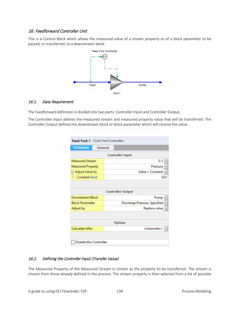
A guide to using OLI Flowsheet: ESP 138 Process Modeling
16. Feedforward Controller Unit
This is a Control Block which allows the measured value of a stream property or of a block parameter to be passed, or transferred, to a downstream block.
16.1. Data Requirement
The Feedforward definition is divided into two parts: Controller Input and Controller Output.
The Controller Input defines the measured stream and measured property value that will be transferred. The Controller Output defines the downstream block or block parameter which will receive the value.
16.2. Defining the Controller Input (Transfer Value)
The Measured Property of the Measured Stream is chosen as the property to be transferred. The stream is chosen from those already defined in the process. The stream property is then selected from a list of possible
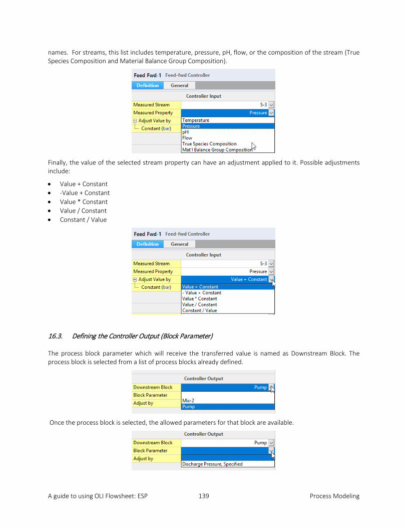
A guide to using OLI Flowsheet: ESP 139 Process Modeling
names. For streams, this list includes temperature, pressure, pH, flow, or the composition of the stream (True Species Composition and Material Balance Group Composition).
Finally, the value of the selected stream property can have an adjustment applied to it. Possible adjustments include:
• Value + Constant • -Value + Constant • Value * Constant • Value / Constant • Constant / Value
16.3. Defining the Controller Output (Block Parameter)
The process block parameter which will receive the transferred value is named as Downstream Block. The process block is selected from a list of process blocks already defined.
Once the process block is selected, the allowed parameters for that block are available.

A guide to using OLI Flowsheet: ESP 140 Process Modeling
Finally, the value of the selected Block Parameter can have an adjustment applied to it. Possible adjustments include:
• Replace value • Add to value • Subtract from value • Multiply times value • Divide value
16.4. Guidelines
1. Avoid trying to control a variable which is discontinuous. For example, avoid trying to reach the saturation point of a solution with respect to a solid.
2. OLI Flowsheet: ESP allows for controlling and tearing the same stream.
17. Manipulator Unit
This is a Control Block which allows the mixing of up to 7 feed streams adiabatically. Either the resulting flow or individual components can be multiplied by a factor. The resulting phase separation and speciation within each phase of the outlet stream is computed.
17.1. Data Requirement
The unit's stream inflow and exit flow must all be given distinct names. This enables streams and units to be recognized and linked together when building a complex process. A minimum of one feed stream and their respective temperature, pressure, flow and composition must be defined by the user.
17.2. Unit Parameters
The Properties pane allows the user to specify the factors by which either the Total Flow or Stream Component composition of the exit stream can be multiplied.
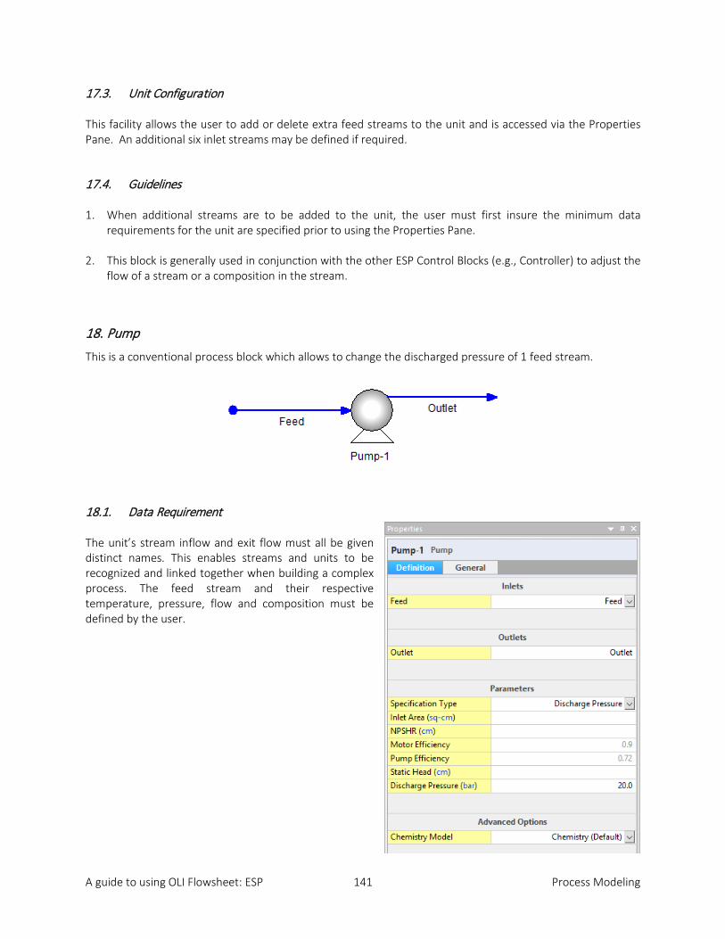
A guide to using OLI Flowsheet: ESP 141 Process Modeling
17.3. Unit Configuration
This facility allows the user to add or delete extra feed streams to the unit and is accessed via the Properties Pane. An additional six inlet streams may be defined if required.
17.4. Guidelines
1. When additional streams are to be added to the unit, the user must first insure the minimum data requirements for the unit are specified prior to using the Properties Pane.
2. This block is generally used in conjunction with the other ESP Control Blocks (e.g., Controller) to adjust the flow of a stream or a composition in the stream.
18. Pump
This is a conventional process block which allows to change the discharged pressure of 1 feed stream.
18.1. Data Requirement
The unit’s stream inflow and exit flow must all be given distinct names. This enables streams and units to be recognized and linked together when building a complex process. The feed stream and their respective temperature, pressure, flow and composition must be defined by the user.

A guide to using OLI Flowsheet: ESP 142 Process Modeling
18.2. Unit Parameters
The parameters available to define the pump are as follows:
Parameter Value Comment
Specification Type Discharged Pressure or Pump Curve Must provide
Inlet Area User Optional
NPSHR* User Optional
Motor Efficiency User (0.0 to 1.0) Default = 0.9
Pump Efficiency User (0.0 to 1.0) Default = 0.72
Static Head User Optional
Discharge Pressure User Must provide
Pump Curve User Must provide
*Net Positive Suction Head Required
To add a Pump Curve, go to Edit Button:
19. RO Membranes (Reverse Osmosis)
This is a process block which allows for the separation of salts from a single process feed stream through the use of a semi-permeable membrane. As a result of this separation, two product streams result one called the “concentrate stream” and the other called the “permeate stream.” The specification of a permeate inlet stream is optional.
19.1. Data Requirement
The unit’s stream inflow(s) and exit flows must be given distinct names. This enables streams and units to be recognized and linked together when building a complex process. A minimum of one conventional feed stream

A guide to using OLI Flowsheet: ESP 143 Process Modeling
and one additional, optional permeate feed stream, together with their conditions must be defined by the user or said stream must be a product stream from another process block.
19.2. Unit Parameters
The parameters available in the Properties Panel are divided in the following:
1. Inlets and Outlets 2. Membrane Element Performance Data 3. Operation Parameters 4. pH Control (Optional) 5. Advanced Options
1. Inlets and Outlets: Clicking the inlets and outlets button, it will bring a new pane where the connections in and out of the RO block can be modified.

A guide to using OLI Flowsheet: ESP 144 Process Modeling
2. Membrane Element Performance Data: Clicking on the Membrane Element Performance Data button, it will bring a new pane where you can input the following information:
In this option, you can select either Manufacturer Data Sheet or Lab analysis. When Manufacturer Data Sheet is selected the user needs to specify the Manufactures and the Model of the membrane. Different options for manufacturer and model will be also displayed. Additionally, active area, permeate flow, permeate recovery, temperature and applied pressure values must be provided.
Salt concentration and Rejections: The user has the option to select specific salts and define their concentration and rejection percentage.
Membrane Model Library: This option allows to save the specified data to Library.
Note: If the user has selected the Manufacturer Option, the test rejection components will have species selection as a Molecular format. On the other hand, if the user selects the Lab Analysis Option, the salt concentration and rejection components will have species selection as Ionic format.
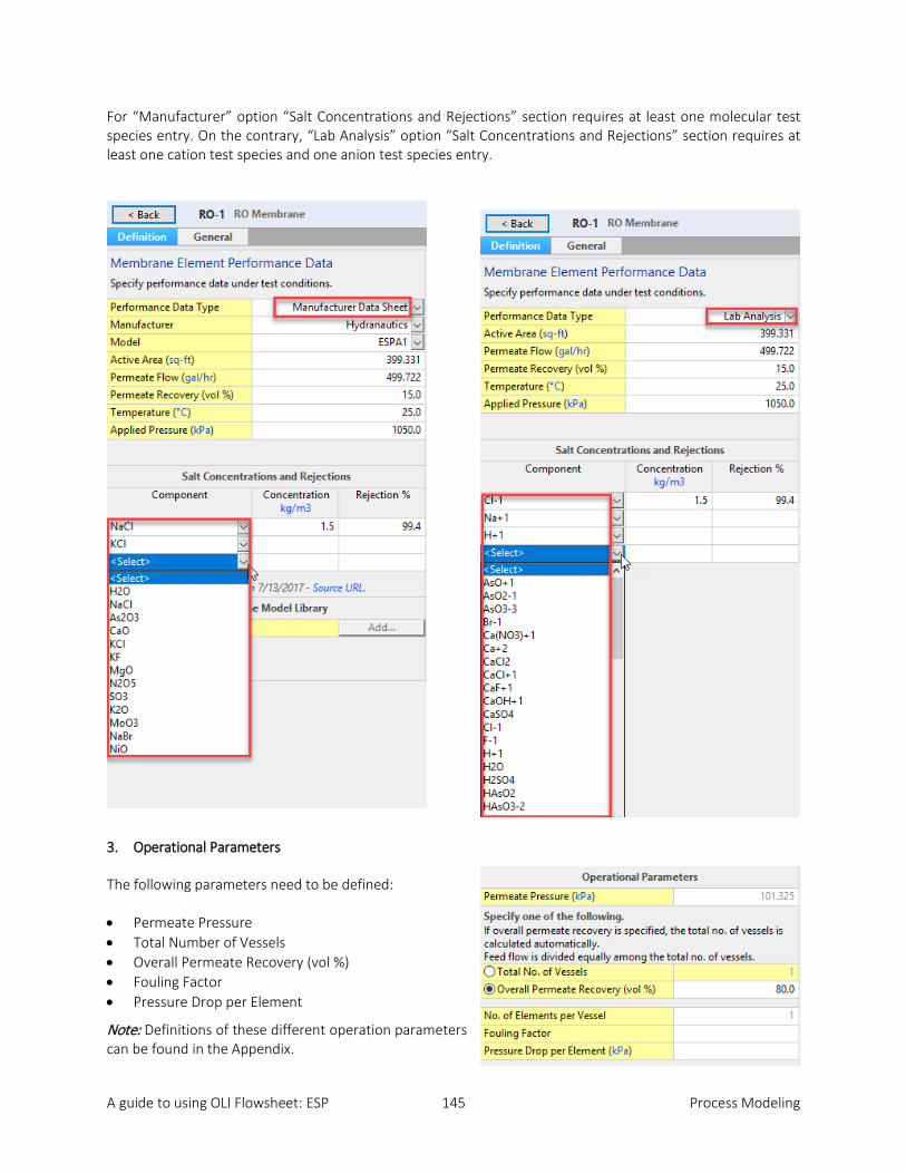
A guide to using OLI Flowsheet: ESP 145 Process Modeling
For “Manufacturer” option “Salt Concentrations and Rejections” section requires at least one molecular test species entry. On the contrary, “Lab Analysis” option “Salt Concentrations and Rejections” section requires at least one cation test species and one anion test species entry.
3. Operational Parameters
The following parameters need to be defined:
• Permeate Pressure • Total Number of Vessels • Overall Permeate Recovery (vol %) • Fouling Factor • Pressure Drop per Element
Note: Definitions of these different operation parameters can be found in the Appendix.
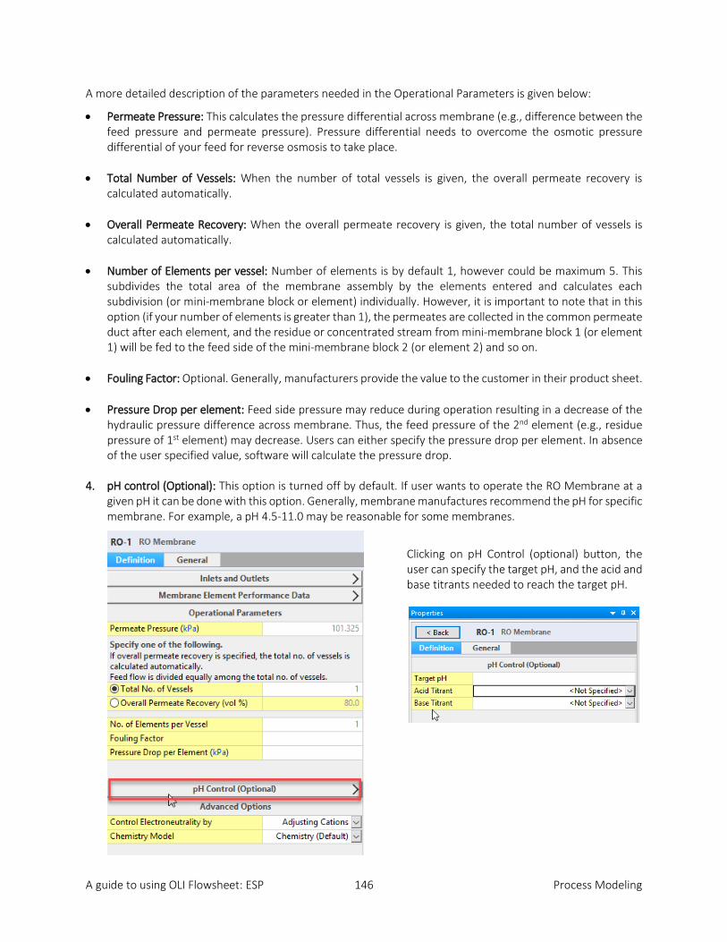
A guide to using OLI Flowsheet: ESP 146 Process Modeling
A more detailed description of the parameters needed in the Operational Parameters is given below:
• Permeate Pressure: This calculates the pressure differential across membrane (e.g., difference between the feed pressure and permeate pressure). Pressure differential needs to overcome the osmotic pressure differential of your feed for reverse osmosis to take place.
• Total Number of Vessels: When the number of total vessels is given, the overall permeate recovery is calculated automatically.
• Overall Permeate Recovery: When the overall permeate recovery is given, the total number of vessels is
calculated automatically.
• Number of Elements per vessel: Number of elements is by default 1, however could be maximum 5. This subdivides the total area of the membrane assembly by the elements entered and calculates each subdivision (or mini-membrane block or element) individually. However, it is important to note that in this option (if your number of elements is greater than 1), the permeates are collected in the common permeate duct after each element, and the residue or concentrated stream from mini-membrane block 1 (or element 1) will be fed to the feed side of the mini-membrane block 2 (or element 2) and so on.
• Fouling Factor: Optional. Generally, manufacturers provide the value to the customer in their product sheet.
• Pressure Drop per element: Feed side pressure may reduce during operation resulting in a decrease of the
hydraulic pressure difference across membrane. Thus, the feed pressure of the 2nd element (e.g., residue pressure of 1st element) may decrease. Users can either specify the pressure drop per element. In absence of the user specified value, software will calculate the pressure drop.
4. pH control (Optional): This option is turned off by default. If user wants to operate the RO Membrane at a given pH it can be done with this option. Generally, membrane manufactures recommend the pH for specific membrane. For example, a pH 4.5-11.0 may be reasonable for some membranes.
Clicking on pH Control (optional) button, the user can specify the target pH, and the acid and base titrants needed to reach the target pH.
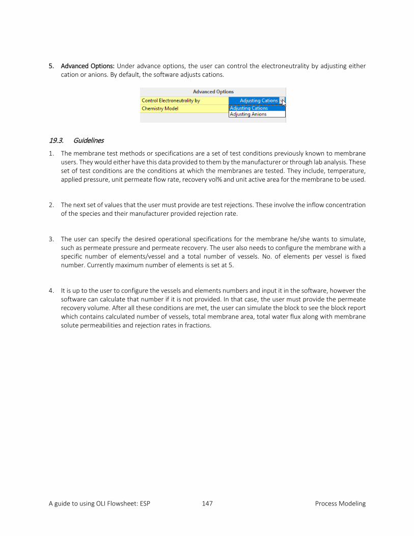
A guide to using OLI Flowsheet: ESP 147 Process Modeling
5. Advanced Options: Under advance options, the user can control the electroneutrality by adjusting either cation or anions. By default, the software adjusts cations.
19.3. Guidelines
1. The membrane test methods or specifications are a set of test conditions previously known to membrane users. They would either have this data provided to them by the manufacturer or through lab analysis. These set of test conditions are the conditions at which the membranes are tested. They include, temperature, applied pressure, unit permeate flow rate, recovery vol% and unit active area for the membrane to be used.
2. The next set of values that the user must provide are test rejections. These involve the inflow concentration of the species and their manufacturer provided rejection rate.
3. The user can specify the desired operational specifications for the membrane he/she wants to simulate, such as permeate pressure and permeate recovery. The user also needs to configure the membrane with a specific number of elements/vessel and a total number of vessels. No. of elements per vessel is fixed number. Currently maximum number of elements is set at 5.
4. It is up to the user to configure the vessels and elements numbers and input it in the software, however the software can calculate that number if it is not provided. In that case, the user must provide the permeate recovery volume. After all these conditions are met, the user can simulate the block to see the block report which contains calculated number of vessels, total membrane area, total water flux along with membrane solute permeabilities and rejection rates in fractions.
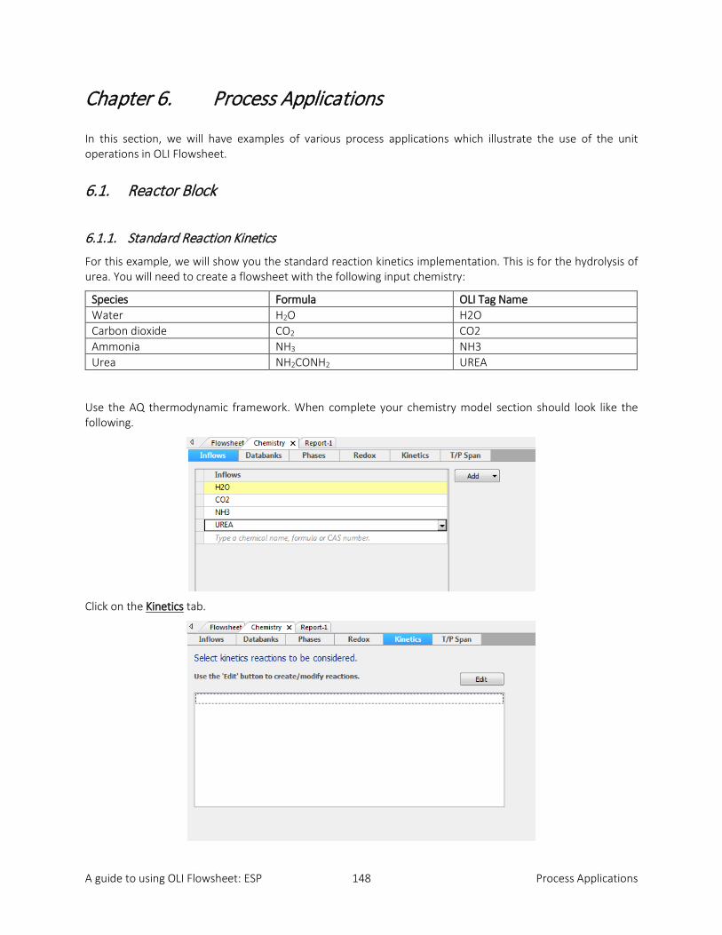
A guide to using OLI Flowsheet: ESP 148 Process Applications
Chapter 6. Process Applications
In this section, we will have examples of various process applications which illustrate the use of the unit operations in OLI Flowsheet.
6.1. Reactor Block
6.1.1. Standard Reaction Kinetics
For this example, we will show you the standard reaction kinetics implementation. This is for the hydrolysis of urea. You will need to create a flowsheet with the following input chemistry:
Species Formula OLI Tag Name Water H2O H2O Carbon dioxide CO2 CO2 Ammonia NH3 NH3 Urea NH2CONH2 UREA
Use the AQ thermodynamic framework. When complete your chemistry model section should look like the following.
Click on the Kinetics tab.
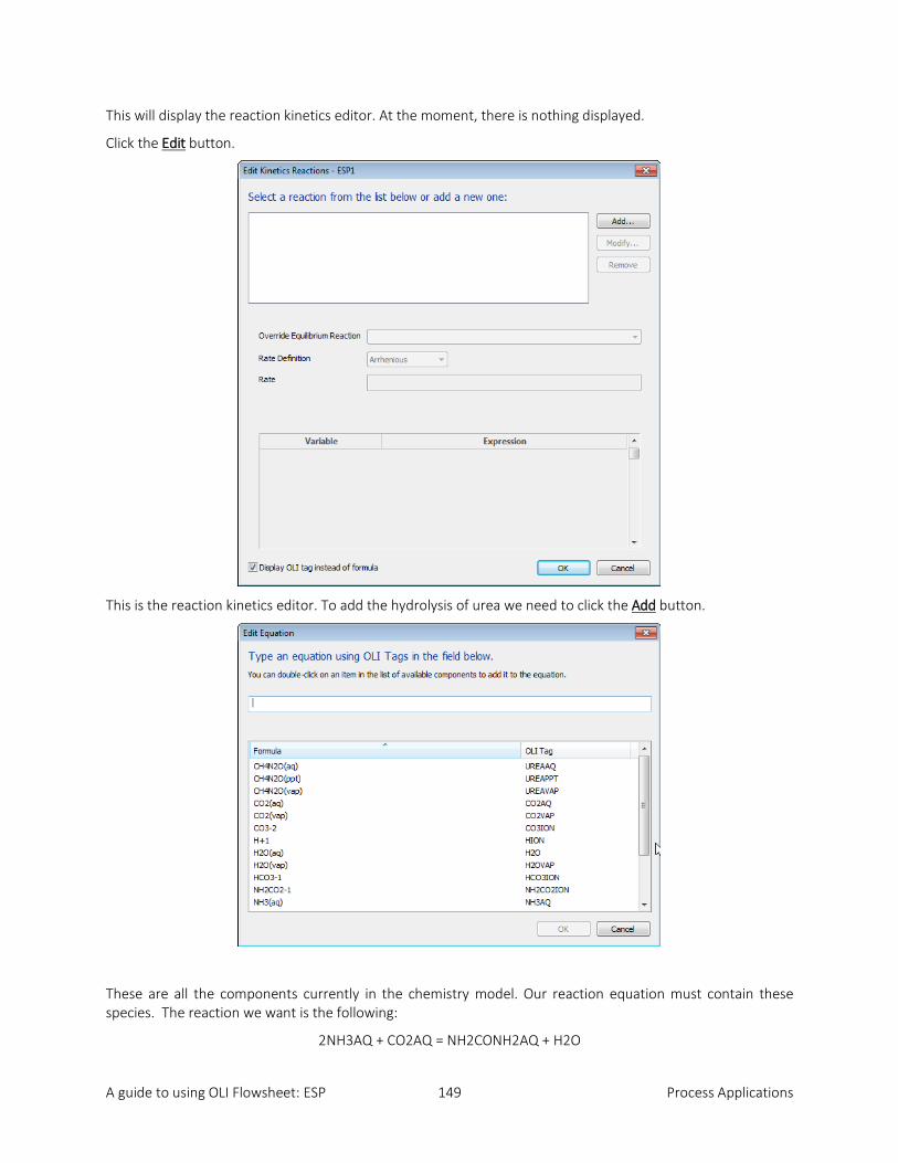
A guide to using OLI Flowsheet: ESP 149 Process Applications
This will display the reaction kinetics editor. At the moment, there is nothing displayed.
Click the Edit button.
This is the reaction kinetics editor. To add the hydrolysis of urea we need to click the Add button.
These are all the components currently in the chemistry model. Our reaction equation must contain these species. The reaction we want is the following:
2NH3AQ + CO2AQ = NH2CONH2AQ + H2O

A guide to using OLI Flowsheet: ESP 150 Process Applications
Let’s start by locating NH3(AQ) from the list:
Double-click the component to add it to the equation.
You can see that we have entered the component but there is an error message. This is ok for now since we haven’t completed the equation. We now need to add the plus sign “+” to add the next component:
Now locate CO2(AQ) from the list and add it in the same manner. After that complete the equation so it looks like the following:
There seems to be a problem. The program will check to see if the equation mass-balances and in this case, it does not. This is because it takes two molecules of ammonia to make urea. You can add the “2” in front of the NH3AQ variable:

A guide to using OLI Flowsheet: ESP 151 Process Applications
Click the OK button to close the editor.
We now have a reaction in the model. We now must change some constants which we get from the literature.
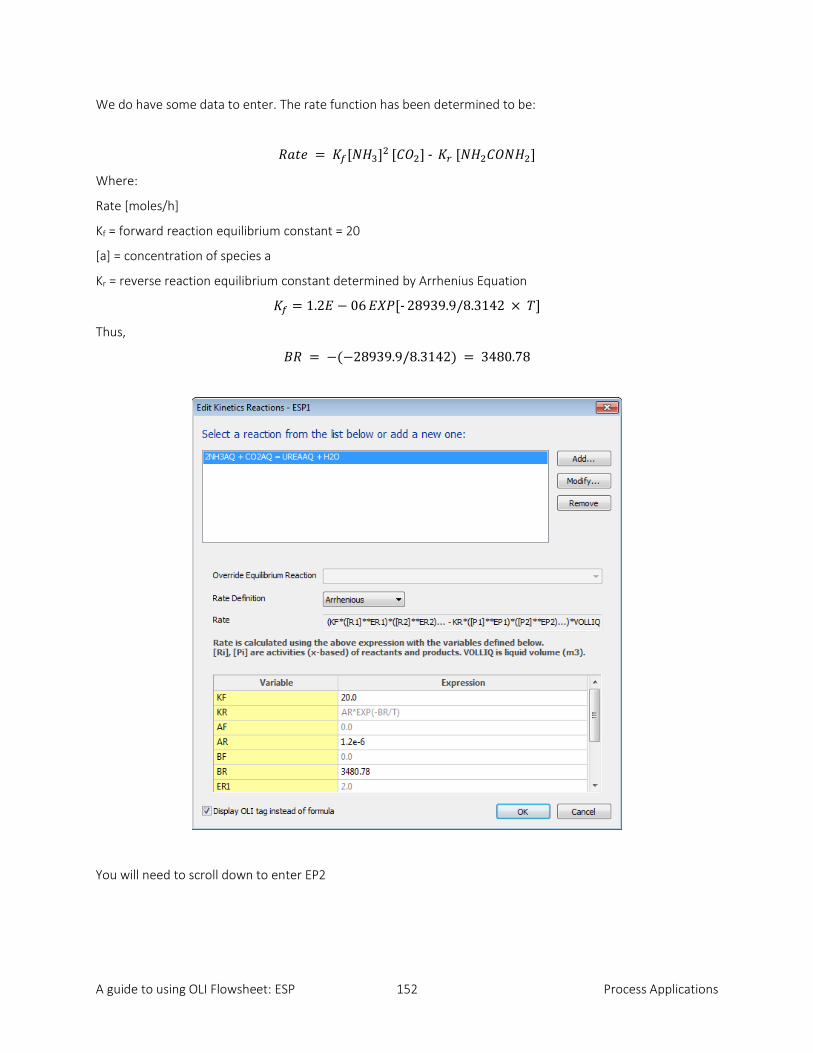
A guide to using OLI Flowsheet: ESP 152 Process Applications
We do have some data to enter. The rate function has been determined to be:
𝑅𝑅𝑎𝑎𝑅𝑅𝑅𝑅 = 𝐾𝐾𝑓𝑓[𝑁𝑁𝐻𝐻3]2 [𝐶𝐶𝑂𝑂2] - 𝐾𝐾𝑟𝑟 [𝑁𝑁𝐻𝐻2𝐶𝐶𝑂𝑂𝑁𝑁𝐻𝐻2]
Where:
Rate [moles/h]
Kf = forward reaction equilibrium constant = 20
[a] = concentration of species a
Kr = reverse reaction equilibrium constant determined by Arrhenius Equation
𝐾𝐾𝑓𝑓 = 1.2𝐸𝐸 − 06 𝐸𝐸𝑋𝑋𝐴𝐴[- 28939.9/8.3142 × 𝑃𝑃]
Thus,
𝑁𝑁𝑅𝑅 = −(−28939.9/8.3142) = 3480.78
You will need to scroll down to enter EP2

A guide to using OLI Flowsheet: ESP 153 Process Applications
Click OK when done.
You will now need to enable the added reaction kinetics.
Check the box if it is not already checked.
Now click on the Flowsheet tab to begin entering the blocks and streams.
Create a flowsheet with a rector block with a single feed stream and a single product stream such as the following:
Enter the following feed parameters given in the table below:
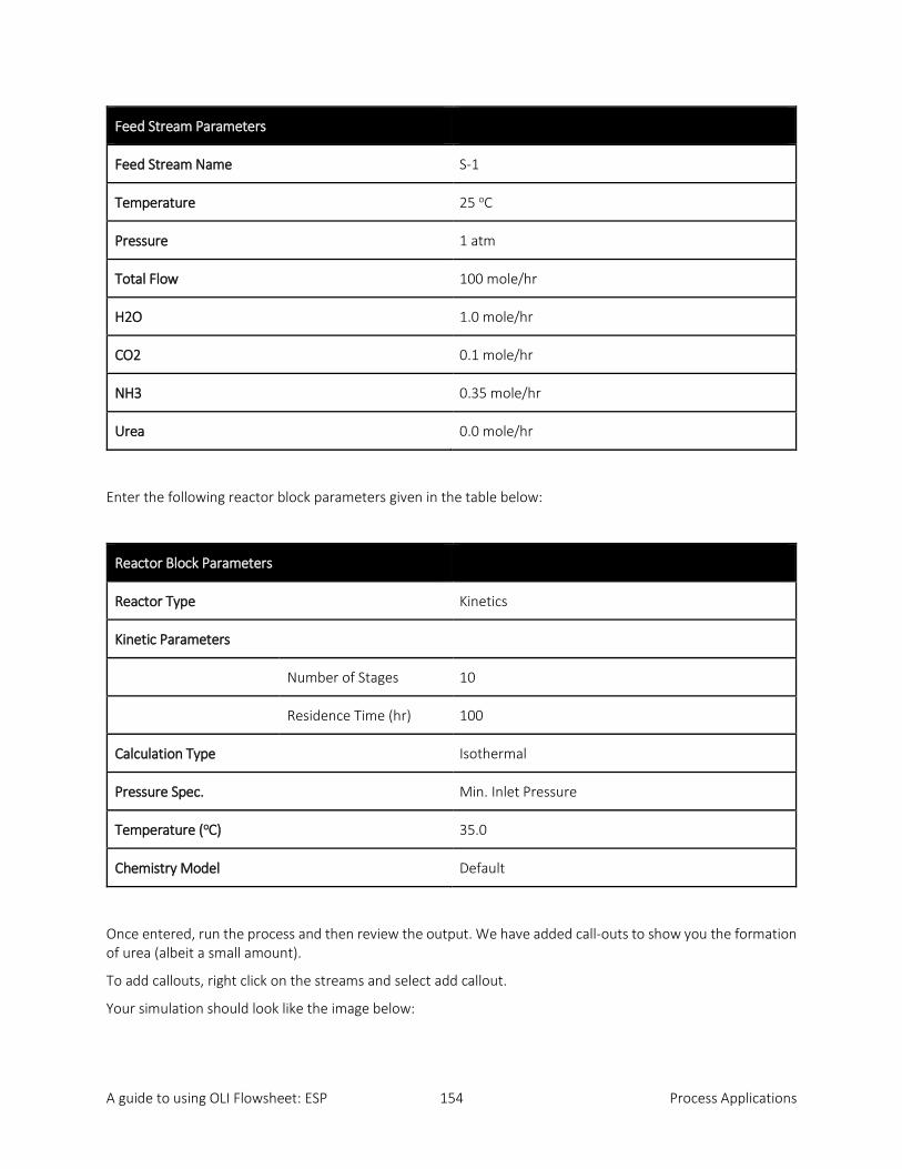
A guide to using OLI Flowsheet: ESP 154 Process Applications
Feed Stream Parameters
Feed Stream Name S-1
Temperature 25 oC
Pressure 1 atm
Total Flow 100 mole/hr
H2O 1.0 mole/hr
CO2 0.1 mole/hr
NH3 0.35 mole/hr
Urea 0.0 mole/hr
Enter the following reactor block parameters given in the table below:
Reactor Block Parameters
Reactor Type Kinetics
Kinetic Parameters
Number of Stages 10
Residence Time (hr) 100
Calculation Type Isothermal
Pressure Spec. Min. Inlet Pressure
Temperature (oC) 35.0
Chemistry Model Default
Once entered, run the process and then review the output. We have added call-outs to show you the formation of urea (albeit a small amount).
To add callouts, right click on the streams and select add callout.
Your simulation should look like the image below:

A guide to using OLI Flowsheet: ESP 155 Process Applications
6.1.2. Non-Standard (User Defined) Reaction Kinetics
In this example, we are using non-standard reaction kinetics to hydrolyze ammonia. The overall reaction is:
𝑵𝑵𝑵𝑵𝟑𝟑(𝒂𝒂𝒂𝒂) + 𝑵𝑵𝟐𝟐𝑶𝑶 ⇌ 𝑵𝑵𝑵𝑵𝟒𝟒+ + 𝑶𝑶𝑵𝑵−
We know the forward rate constant (and hence the forward reaction rate) but we wish to constrain the forward and reverse reaction rates to the thermodynamic equilibrium constant stored in the OLI Databases.
Create a chemistry section with the following information:
Non-Standard Reaction Kinetics
Thermodynamic Framework Aqueous (H+ Ion)
Additional Databanks None
Phases Default
Redox Off
Inflows Formula OLI Tag Name
Water H2O H2O
Ammonia NH3 NH3
Using the techniques from the previous section, add the kinetics reaction for the reaction shown above.
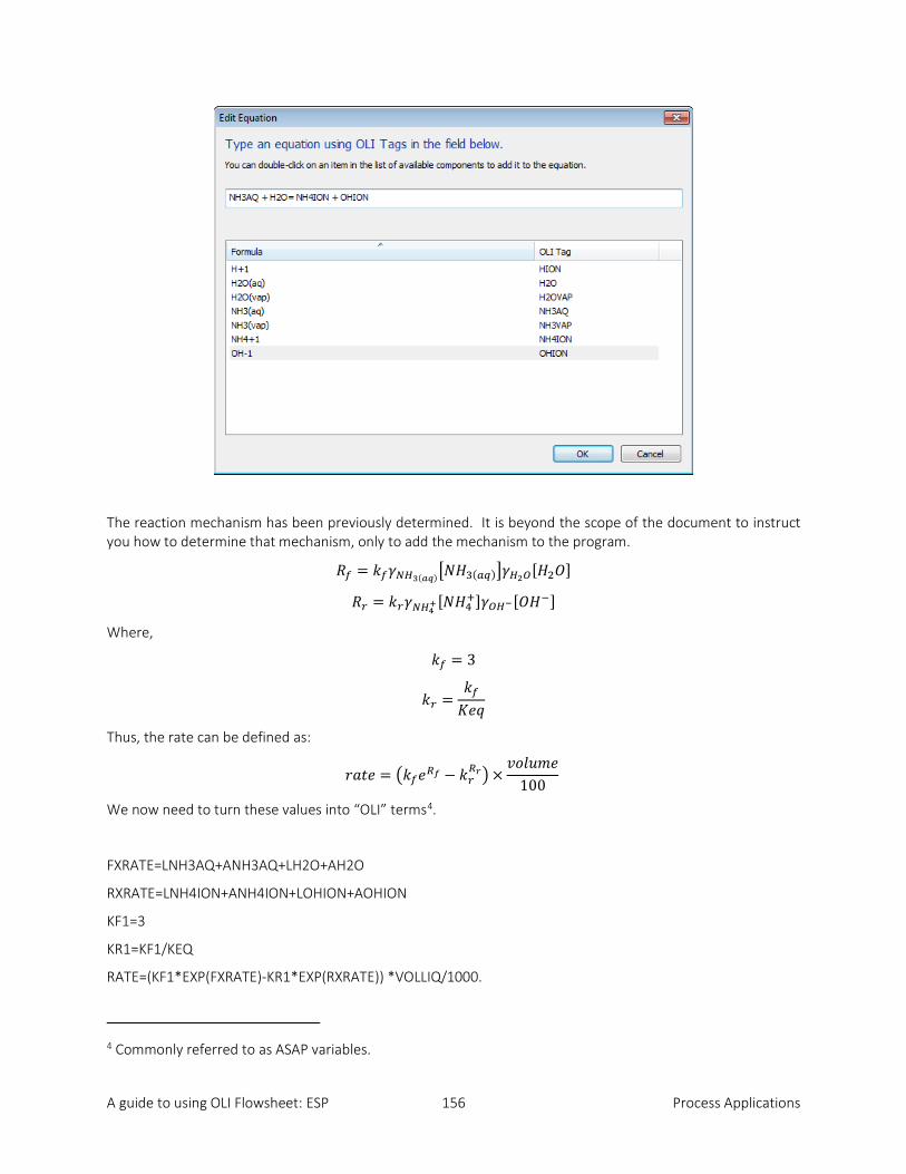
A guide to using OLI Flowsheet: ESP 156 Process Applications
The reaction mechanism has been previously determined. It is beyond the scope of the document to instruct you how to determine that mechanism, only to add the mechanism to the program.
𝑅𝑅𝑓𝑓 = 𝑘𝑘𝑓𝑓𝛾𝛾𝑁𝑁𝐻𝐻3(𝑎𝑎𝑎𝑎)�𝑁𝑁𝐻𝐻3(𝑎𝑎𝑎𝑎)�𝛾𝛾𝐻𝐻2𝑂𝑂[𝐻𝐻2𝑂𝑂]
𝑅𝑅𝑟𝑟 = 𝑘𝑘𝑟𝑟𝛾𝛾𝑁𝑁𝐻𝐻4+[𝑁𝑁𝐻𝐻4+]𝛾𝛾𝑂𝑂𝐻𝐻−[𝑂𝑂𝐻𝐻−]
Where,
𝑘𝑘𝑓𝑓 = 3
𝑘𝑘𝑟𝑟 =𝑘𝑘𝑓𝑓𝐾𝐾𝑅𝑅𝐾𝐾
Thus, the rate can be defined as:
𝑟𝑟𝑎𝑎𝑅𝑅𝑅𝑅 = �𝑘𝑘𝑓𝑓𝑅𝑅𝑅𝑅𝑓𝑓 − 𝑘𝑘𝑟𝑟𝑅𝑅𝑟𝑟�×
𝑣𝑣𝑉𝑉𝑙𝑙𝑣𝑣𝑚𝑚𝑅𝑅100
We now need to turn these values into “OLI” terms4.
FXRATE=LNH3AQ+ANH3AQ+LH2O+AH2O
RXRATE=LNH4ION+ANH4ION+LOHION+AOHION
KF1=3
KR1=KF1/KEQ
RATE=(KF1*EXP(FXRATE)-KR1*EXP(RXRATE)) *VOLLIQ/1000.
4 Commonly referred to as ASAP variables.

A guide to using OLI Flowsheet: ESP 157 Process Applications
Clicking OK will return you to the editor:
You will notice that we are replacing an existing equilibrium equation with reaction kinetics (unlike the previous example where we created a new equation.)

A guide to using OLI Flowsheet: ESP 158 Process Applications
The reaction kinetics we have for this example is not Arrhenius. Change the Rate Definition button to User Defined.
We first must enter our variables and expressions in the lower half of the dialog. Each variable must be on a separate row.

A guide to using OLI Flowsheet: ESP 159 Process Applications
You now must enter the overall rate expression in the box marked Rate.
Click ok to accept this information.
Enable the kinetics reaction by checking the box.
Return now to the flowsheet.
Create a flowsheet with a rector block with a single feed stream and a single product stream such as the following:
Enter the following for the feed stream parameters:
Feed Stream Parameters
Feed Stream Name S-1
Temperature 25 oC
Pressure 1 atm
Total Flow Automatic

A guide to using OLI Flowsheet: ESP 160 Process Applications
H2O 55.5087 mole/hr
NH3 0.1 mole/hr
Enter the following for the Reactor block parameters:
Reactor Block Parameters
Reactor Type Kinetics
Kinetic Parameters
Number of Stages 10
Residence Time (hr) 100
Calculation Type Isothermal
Pressure Spec. Min. Inlet Pressure
Temperature (oC) 25.0
Chemistry Model Default
Run the process.
Here we have displayed the output of the process using callouts:
The stream S-1 represents the equilibrium condition. The stream pH is approximately 7.0. The stream S-2 represents the condition with reaction kinetics limiting the reforming of ammonia from the ammonium ion. The pH is much higher at approximate 10.7 which shows that it is not at equilibrium.
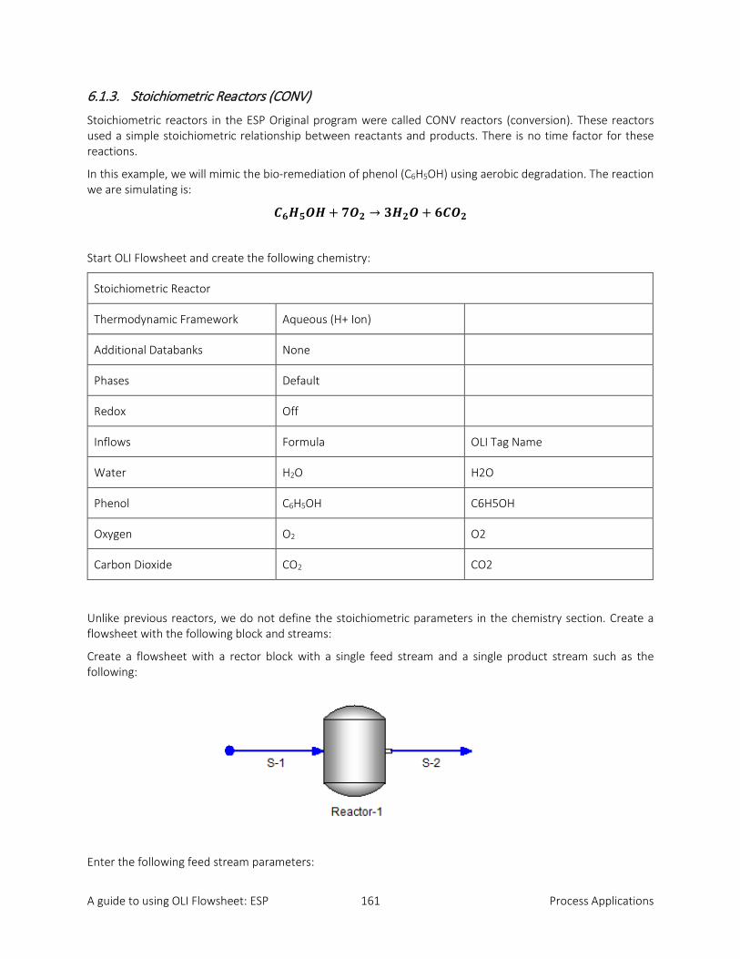
A guide to using OLI Flowsheet: ESP 161 Process Applications
6.1.3. Stoichiometric Reactors (CONV)
Stoichiometric reactors in the ESP Original program were called CONV reactors (conversion). These reactors used a simple stoichiometric relationship between reactants and products. There is no time factor for these reactions.
In this example, we will mimic the bio-remediation of phenol (C6H5OH) using aerobic degradation. The reaction we are simulating is:
𝑪𝑪𝟔𝟔𝑵𝑵𝟓𝟓𝑶𝑶𝑵𝑵 + 𝟕𝟕𝑶𝑶𝟐𝟐 → 𝟑𝟑𝑵𝑵𝟐𝟐𝑶𝑶 + 𝟔𝟔𝑪𝑪𝑶𝑶𝟐𝟐
Start OLI Flowsheet and create the following chemistry:
Stoichiometric Reactor
Thermodynamic Framework Aqueous (H+ Ion)
Additional Databanks None
Phases Default
Redox Off
Inflows Formula OLI Tag Name
Water H2O H2O
Phenol C6H5OH C6H5OH
Oxygen O2 O2
Carbon Dioxide CO2 CO2
Unlike previous reactors, we do not define the stoichiometric parameters in the chemistry section. Create a flowsheet with the following block and streams:
Create a flowsheet with a rector block with a single feed stream and a single product stream such as the following:
Enter the following feed stream parameters:
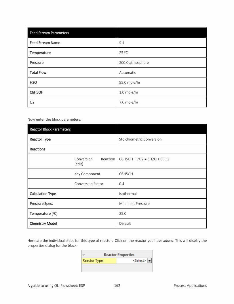
A guide to using OLI Flowsheet: ESP 162 Process Applications
Feed Stream Parameters
Feed Stream Name S-1
Temperature 25 oC
Pressure 200.0 atmosphere
Total Flow Automatic
H2O 55.0 mole/hr
C6H5OH 1.0 mole/hr
O2 7.0 mole/hr
Now enter the block parameters:
Reactor Block Parameters
Reactor Type Stoichiometric Conversion
Reactions
Conversion Reaction (edit)
C6H5OH + 7O2 = 3H2O + 6CO2
Key Component C6H5OH
Conversion factor 0.4
Calculation Type Isothermal
Pressure Spec. Min. Inlet Pressure
Temperature (oC) 25.0
Chemistry Model Default
Here are the individual steps for this type of reactor. Click on the reactor you have added. This will display the properties dialog for the block:

A guide to using OLI Flowsheet: ESP 163 Process Applications
Change the type of reactor to Stoichiometric Conversion.
Click on the Reactions button. This will display a fly-out dialog.
This brings up a familiar dialog. Normally we used this dialog in the chemistry section but now we are using the same dialog in the block.
Click the Add button.

A guide to using OLI Flowsheet: ESP 164 Process Applications
As we did in the previous section, we will now add the equation from above.
Click OK
We now must define the key reactant. This is what the conversion is based on. Select phenol (C6H5OH).
For our purposes we are converting 40% (on a mole basis) so enter 0.4
Click OK to continue.
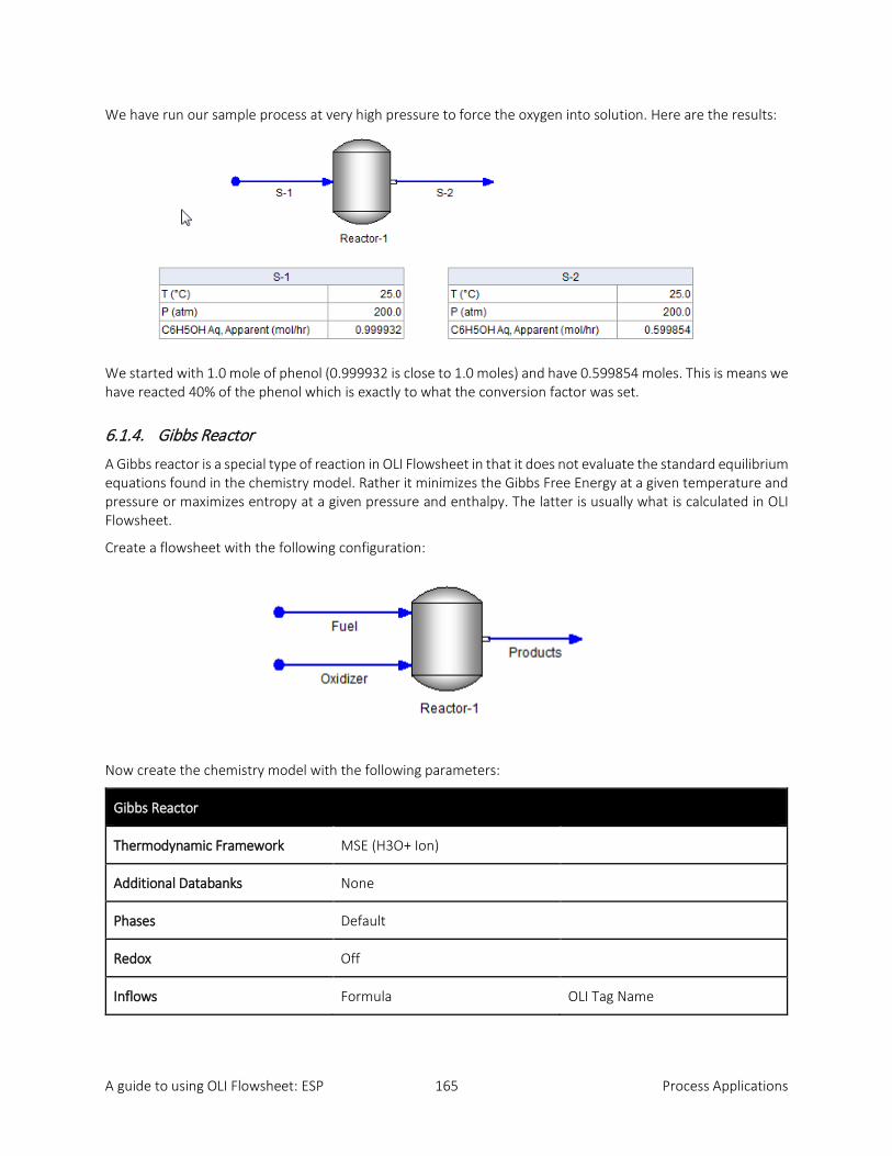
A guide to using OLI Flowsheet: ESP 165 Process Applications
We have run our sample process at very high pressure to force the oxygen into solution. Here are the results:
We started with 1.0 mole of phenol (0.999932 is close to 1.0 moles) and have 0.599854 moles. This is means we have reacted 40% of the phenol which is exactly to what the conversion factor was set.
6.1.4. Gibbs Reactor
A Gibbs reactor is a special type of reaction in OLI Flowsheet in that it does not evaluate the standard equilibrium equations found in the chemistry model. Rather it minimizes the Gibbs Free Energy at a given temperature and pressure or maximizes entropy at a given pressure and enthalpy. The latter is usually what is calculated in OLI Flowsheet.
Create a flowsheet with the following configuration:
Now create the chemistry model with the following parameters:
Gibbs Reactor
Thermodynamic Framework MSE (H3O+ Ion)
Additional Databanks None
Phases Default
Redox Off
Inflows Formula OLI Tag Name

A guide to using OLI Flowsheet: ESP 166 Process Applications
Water H2O H2O
Methane CH4 CH4
Oxygen O2 O2
Carbon Dioxide CO2 CO2
Nitrogen N2 N2
Carbon Monoxide CO CO
Now enter the parameters for each inlet stream:
Feed Stream Parameters
Feed Stream Name Fuel
Temperature 25 oC
Pressure 1.0 Atm
Total Flow 1 m3/hr m3/hr
H2O 0.0 mole/hr mole/hr
CH4 100.0 mole/hr
O2 0 mole/hr
CO2 0 mole/hr
N2 0 mole/hr
CO 0 mole/hr
Feed Stream Parameters
Feed Stream Name Oxidizer
Temperature 25 oC
Pressure 1.0 Atm
Total Flow 0.1 m3/hr m3/hr

A guide to using OLI Flowsheet: ESP 167 Process Applications
H2O 0.0 mole/hr mole/hr
CH4 0.0 mole/hr
O2 20 mole/hr
CO2 0 mole/hr
N2 80 mole/hr
CO 0 mole/hr
Now enter the block parameters for the reactors. We will describe the details about the new parameters after the table.
Reactor Block Parameters
Reactor Type Gibbs
Reacting Vapor Species
CH4 Enabled
CO Enabled
CO2 Enabled
H2O Enabled
N2 Disabled
O2 Enabled
Calculation Type Adiabatic
Pressure Spec. Min. Inlet Pressure
Heat Duty 0.0
Chemistry Model Default
This the type of reactor you need to specify which vapor species can react. In this case, we are simulating a combustion reaction, so we do not require Nitrogen gas to be reactive. After specifying the reactor type we need to enable the gasses.
Click the fly-out button next to Reacting Vapor Species.

A guide to using OLI Flowsheet: ESP 168 Process Applications
Check the following components:
• CH4CO • CO2 • H2O • O2 • Skip N2
Click the Back button and then run the calculation.
The simulation results are presented in the callout tables.
You can see that we have reacted methane with oxygen and have formed the traditional combustion products of carbon dioxide and water. We also have some incomplete combustion and have formed some carbon monoxide at approximately 8 ppm. There has also been a temperature increase.
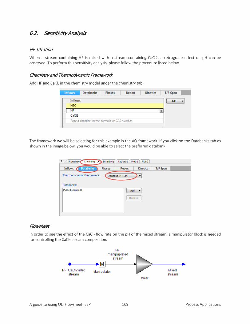
A guide to using OLI Flowsheet: ESP 169 Process Applications
6.2. Sensitivity Analysis
HF Titration
When a stream containing HF is mixed with a stream containing CaCl2, a retrograde effect on pH can be observed. To perform this sensitivity analysis, please follow the procedure listed below.
Chemistry and Thermodynamic Framework
Add HF and CaCl2 in the chemistry model under the chemistry tab:
The framework we will be selecting for this example is the AQ framework. If you click on the Databanks tab as shown in the image below, you would be able to select the preferred databank:
Flowsheet
In order to see the effect of the CaCl2 flow rate on the pH of the mixed stream, a manipulator block is needed for controlling the CaCl2 stream composition.
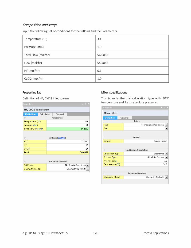
A guide to using OLI Flowsheet: ESP 170 Process Applications
Composition and setup
Input the following set of conditions for the Inflows and the Parameters.
Temperature (°C) 30
Pressure (atm) 1.0
Total Flow (mol/hr) 56.6082
H2O (mol/hr) 55.5082
HF (mol/hr) 0.1
CaCl2 (mol/hr) 1.0
Properties Tab
Definition of HF, CaCl2 inlet stream
Mixer specifications
This is an Isothermal calculation type with 30°C temperature and 1 atm absolute pressure.

A guide to using OLI Flowsheet: ESP 171 Process Applications
Create Analysis
Click on the Analysis option at the top toolbar:
You will see the following screen:
Click on the Add button and select the Block to be Manipulator block.

A guide to using OLI Flowsheet: ESP 172 Process Applications
Drop down on the Block Parameter and select the Flow Factor, CaCl2. Your final screen with the starting value 0.0 and ending value 0.2 with 20 steps specification should match the following image:
Monitored Variables
Now that we have selected the parameters to vary, we would need select the monitored variables in order to create the plot. If you click on the Monitored Variables tab, you will see the following screen, click on the Add button:
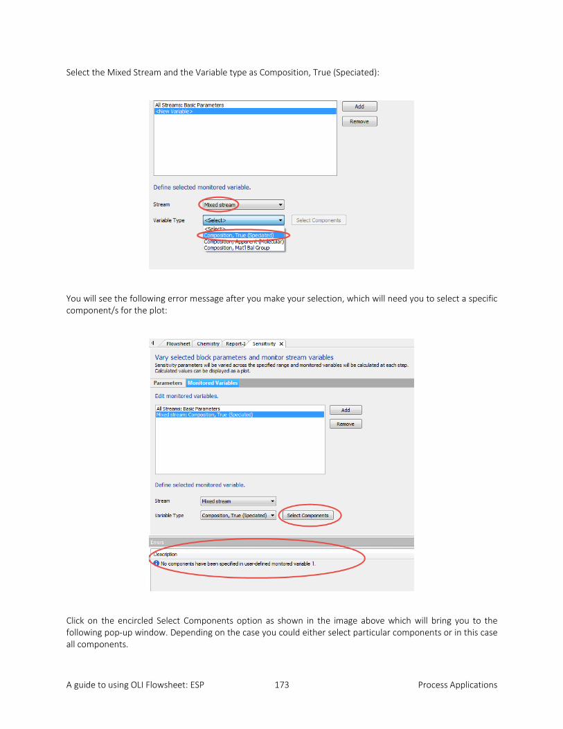
A guide to using OLI Flowsheet: ESP 173 Process Applications
Select the Mixed Stream and the Variable type as Composition, True (Speciated):
You will see the following error message after you make your selection, which will need you to select a specific component/s for the plot:
Click on the encircled Select Components option as shown in the image above which will bring you to the following pop-up window. Depending on the case you could either select particular components or in this case all components.
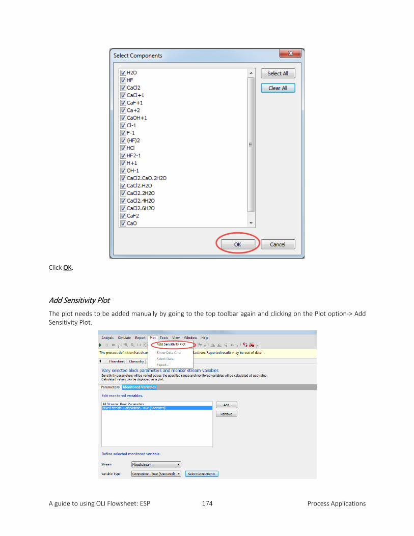
A guide to using OLI Flowsheet: ESP 174 Process Applications
Click OK.
Add Sensitivity Plot
The plot needs to be added manually by going to the top toolbar again and clicking on the Plot option-> Add Sensitivity Plot.

A guide to using OLI Flowsheet: ESP 175 Process Applications
Now you will need to run the file by clicking the Run button or using a shortcut F9.
The default plot has H2O Mixed Stream on Y axis, and you will need to click on Select Data button to customize the plot view.
1. Click on Select Data 2. Select the Stream that you want to plot the stream variables for, in this case , since we are interested
in the pH of the mixed stream , we will select the HF manipulated stream.
Add Mass of Solid phase for the manipulated stream and the pH as shown below:
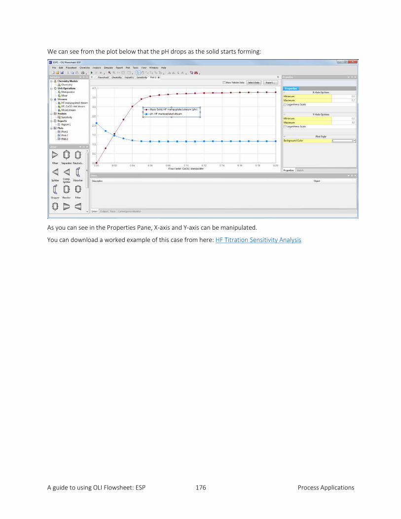
A guide to using OLI Flowsheet: ESP 176 Process Applications
We can see from the plot below that the pH drops as the solid starts forming:
As you can see in the Properties Pane, X-axis and Y-axis can be manipulated.
You can download a worked example of this case from here: HF Titration Sensitivity Analysis

A guide to using OLI Flowsheet: ESP 177 Process Applications
6.3. RO Membranes (Reverse Osmosis)
Overview of RO
This example of an RO membrane compares the OLI Flowsheet simulation with a real-world application. In this case, we are simulating a desalination plant located in the middle-east and built to World Health Organization standard. The overall process flowsheet is shown in the image below:
Flowsheet RO plant5
The goal of this simulation is to confirm that the objective of having a permeate flowrate of a minimum of 3600 m3/day with a TDS (total dissolved solids) less than 100 ppm. The brackish feedwater is over 10,000 TDS.
In this simulation we will concentrate only the pH pretreatment section and the RO membrane itself.
Defining the Chemistry Model
For this simulation we are assuming you already know how to use OLI Flowsheet. We need to first define the chemistry for this process. Start OLI Flowsheet and click on the Chemistry Tab.
5 Source: Abdel-Fatah, M.A., El-Gendi, A and Ashour, F. (2016) Performance Evaluation and Design of RO Desalinatino Plant: Case Study. Journal of Geoscience and Environment Protection, 4, 53-63
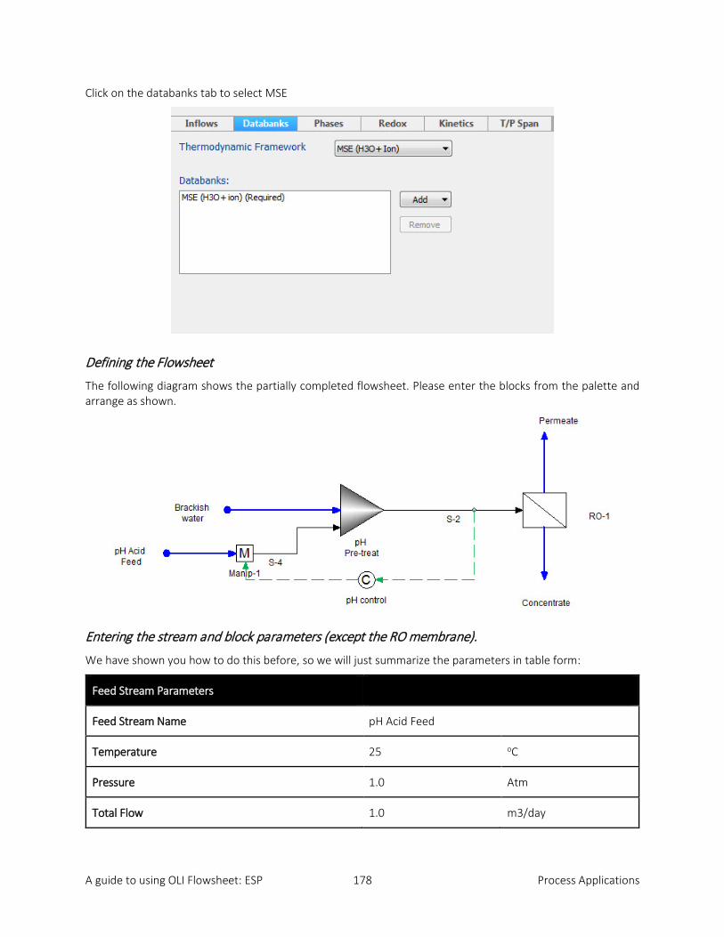
A guide to using OLI Flowsheet: ESP 178 Process Applications
Click on the databanks tab to select MSE
Defining the Flowsheet
The following diagram shows the partially completed flowsheet. Please enter the blocks from the palette and arrange as shown.
Entering the stream and block parameters (except the RO membrane).
We have shown you how to do this before, so we will just summarize the parameters in table form:
Feed Stream Parameters
Feed Stream Name pH Acid Feed
Temperature 25 oC
Pressure 1.0 Atm
Total Flow 1.0 m3/day

A guide to using OLI Flowsheet: ESP 179 Process Applications
H2O 99.0 mass %
CO2 0 mass %
CAO 0 mass %
K2O 0 mass %
MGO 0 mass %
NA2O 0 mass %
NACL 0 mass %
SO3 0 mass %
HCL 1.0 mass %
Feed Stream Parameters
Feed Stream Name Brackish water
Temperature 25 oC
Pressure 1.0 Atm
Total Flow 7200 m3/day
H2O 1323.38 mol/day
CO2 0.176125 mol/day
CAO 0.220969 mol/day
K2O 0.139955 mol/day
MGO 0.16293 mol/day
NA2O 0.0196066 mol/day
NACL 1.6363 mol/day
SO3 0.502502 mol/day
HCL 0.0 mass %
The TDS has been calculated for this stream to be approximately 7400 mg/L

A guide to using OLI Flowsheet: ESP 180 Process Applications
Block Parameters
Block Type Manipulator
Block Name Manip-1
Streams
Inlet pH Acid Feed
Outlet S-4
Parameters
Manipulator Type Total Flow
Factor, Flow 1.0
Chemistry Model Default
Block Parameters
Block Type Mixer
Block Name pH Pre-Treat
Streams
Inlet Brackish Water
Outlet S-2
Parameters
Calculation Type Adiabatic
Pressure Spec. Absolute Pressure
Pressure (Bar) 21.6
Heat Duty (cal/hr) 0
Chemistry Model Default

A guide to using OLI Flowsheet: ESP 181 Process Applications
Block Parameters
Block Type Feedback Controller
Block Name pH Control
Parameters
Target Stream S-2
Spec Type pH
Target Value 6.0
Heat Duty (cal/hr) 0
Control Parameters
Controlling Block Manip-1
Block Parameter Factor, Flow
Options
Calculate After <automatic)
Disable this Controller No (unchecked)

A guide to using OLI Flowsheet: ESP 182 Process Applications
Defining the RO Membrane Block
The RO Membrane block is a relatively complicated block. For this simulation we are using the parameters of a real membrane. The membrane under consideration is DOW FILMTECTM BW30-400 Element6.
There is a lot of data to enter for this simulation. The first is to confirm the Inlets and Outlets.
Click the Back button.
Now, we need to define our RO membrane parameters. Click the Membrane Element Performance Data button.
6 DOW FILMTEC is a registered trademark of the DOW Chemical Company. The parameters were taken from the paper referenced earlier in this section.

A guide to using OLI Flowsheet: ESP 183 Process Applications
The most common source of data will be from a manufacturer’s data sheet. From data sheet we have the following values.
RO Element Data
Active Area (m2) 37.0
Permeate Flow (m3/day) 40
Permeate Recovery (vol %) 15
Temperature (oC) 25
Applied Pressure (bar) 15.5
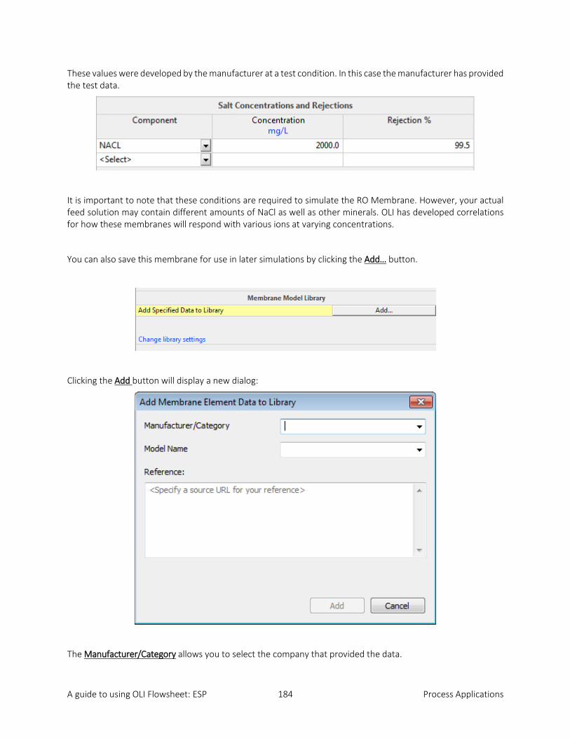
A guide to using OLI Flowsheet: ESP 184 Process Applications
These values were developed by the manufacturer at a test condition. In this case the manufacturer has provided the test data.
It is important to note that these conditions are required to simulate the RO Membrane. However, your actual feed solution may contain different amounts of NaCl as well as other minerals. OLI has developed correlations for how these membranes will respond with various ions at varying concentrations.
You can also save this membrane for use in later simulations by clicking the Add… button.
Clicking the Add button will display a new dialog:
The Manufacturer/Category allows you to select the company that provided the data.
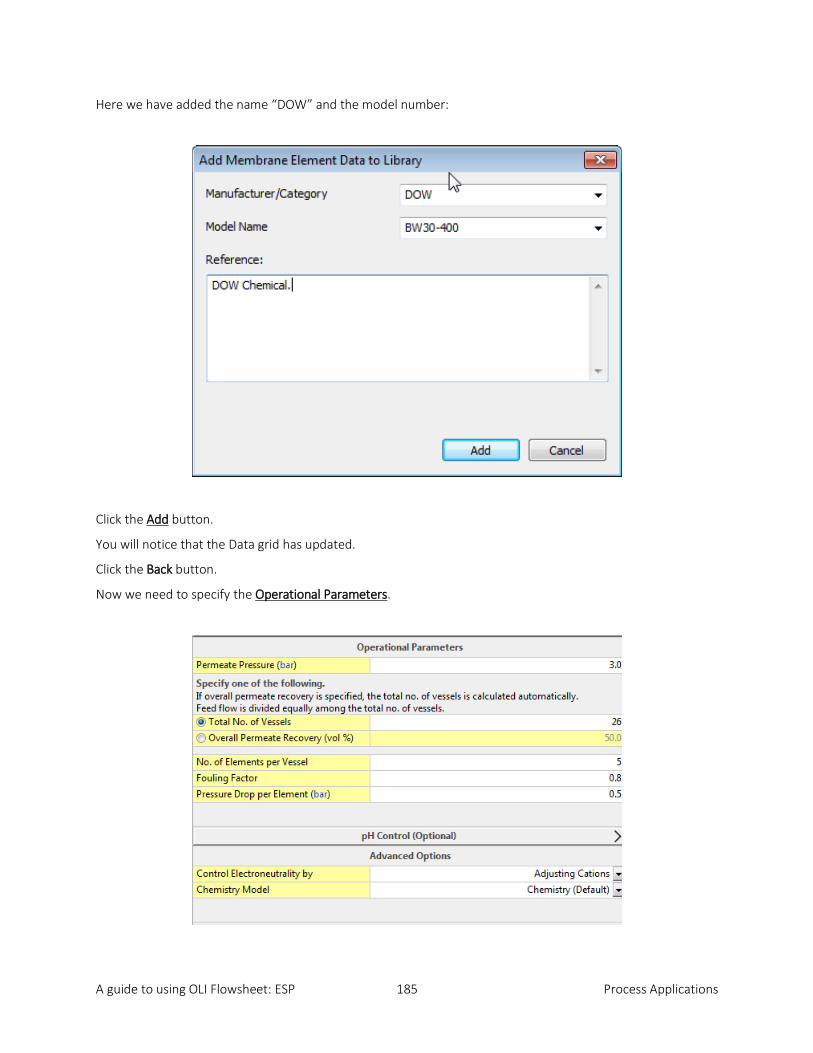
A guide to using OLI Flowsheet: ESP 185 Process Applications
Here we have added the name “DOW” and the model number:
Click the Add button.
You will notice that the Data grid has updated.
Click the Back button.
Now we need to specify the Operational Parameters.

A guide to using OLI Flowsheet: ESP 186 Process Applications
The Permeate Pressure is the pressure on the downstream side of the membrane is usually determined by other operational considerations. The total number of vessels are the actual RO units under consideration. The number of vessels was set by the authors of the paper mentioned previously (Abdel-Fatah, et.al.)
The number of Elements per Vessel was set to 5. The authors of the paper used 6 but that number is outside the range permitted by OLI. The authors set a fouling factor of 0.8 and a pressure drop per element of 0.5 bar.
As the ions move across the membrane there is a mathematical imbalance in electrical charge. The user can specify if the imbalance is corrected by adding/removing cations or anions. Cations are the default value.
At this point the membrane is fully defined and we are ready to run the simulation.
Running the simulation
The simulation was run without any additional tweaks. We have added some call-outs to make our job of analyzing the simulation easier.
The brackish water had an approximately TDS of 7400 mg/L. Remember the World Health Organization wants a TDS of less than 100 mg/L. Reviewing the Permeate stream we can see some values that are of use to us.
One current deficiency is that the TDS value is not automatically calculated by OLI Flowsheet. It is calculated internally but not currently exposed. We can get a quick estimate of the TDS by reporting the concentration of H2O and any volatiles that may be in the stream (in this case CO2).
The approximation for TDS can be calculated as follows:
𝑃𝑃𝑑𝑑𝑆𝑆 �𝑚𝑚𝑚𝑚𝐿𝐿 � = 1,000,000
𝑚𝑚𝑚𝑚𝐿𝐿−𝐻𝐻2𝑂𝑂 �
𝑚𝑚𝑚𝑚𝐿𝐿 � − 𝑣𝑣𝑉𝑉𝑙𝑙𝑎𝑎𝑅𝑅𝑖𝑖𝑙𝑙𝑅𝑅𝑠𝑠 (
𝑚𝑚𝑚𝑚𝐿𝐿
)

A guide to using OLI Flowsheet: ESP 187 Process Applications
The call-out for the Permeate stream has the following values.
So, to calculate TDS we have:
𝑃𝑃𝑑𝑑𝑆𝑆 �𝑚𝑚𝑚𝑚𝐿𝐿 � = 1,000,000
𝑚𝑚𝑚𝑚𝐿𝐿− 9.99722 × 10⁵𝐻𝐻2𝑂𝑂 �
𝑚𝑚𝑚𝑚𝐿𝐿 � − 212 𝐶𝐶𝑂𝑂2 �
𝑚𝑚𝑚𝑚𝐿𝐿 � = 66 𝑚𝑚𝑚𝑚/𝐿𝐿
This certainly achieves the World Health Organization specification of less than 100 mg/L. The authors also wanted to have a permeate flowrate of more than 3600 m3/day and we are reporting slightly more at 3675 m3/day.
This shows that the OLI RO Membrane matches a peer reviewed academic project.
You can download a worked copy of this example from here: RO Membranes
T (°C) 24.5394P (bar) 3.0pH 4.59825Volume (m3/day) 3675.71Os Pres (bar) 0.167249H2O Liq1, True (ppm (mass)) 9.99722e5CO2 Liq1, True (ppm (mass)) 211.895
Permeate

A guide to using OLI Flowsheet: ESP 188 Appendix
Chapter 7. Appendix
OLI MEMBRANE TECHNOLOGY: SIMULATOR FOR REVERSE OSMOSIS PROCESS
Summary
To model the transport mechanism inside the membrane, solution-diffusion approach has been incorporated. In the solution-diffusion model, it is proposed that transfer of ions and water through polymeric membranes occurs via a solution diffusion mechanism because of dissolution of permeates in the membrane materials [1]. The water flux through the membrane is a function of water permeability coefficient, hydrodynamic pressure difference and osmotic pressure difference across the membrane, whereas, the solute flux through the membrane is a function of solute permeability constant and solute concentration gradient across the membrane [2]. Molecular size of the ions strongly affects the transport characteristics of the ions due to the sieving action of the membranes. However, in water environment, different number of water molecules surround each cation and anion. Thus, the real radius of an ion is the one that considers the water molecules around it (i.e., the hydrated ion radius) rather than the absolute ionic crystal radius. Regardless of membrane type, the type of experiment, and the membrane configuration, the salt permeabilities are inversely proportional to the hydrated radii of the ions [3]. In OLI membrane model, permeability of ions has been correlated with their hydration numbers.
In general, the typical order of rejection of cations by reverse osmosis membranes follow Fe3+ > Ni2+ ≈ Cu2+ > Mg2+ > Ca2+ > Na+ > K+, and PO4
3- > SO42- > HCO3
- > Br- > Cl- > NO3- ≈ F- for anions [4]. The permeability of cations
and anions calculated as a function of hydration numbers follow the typical trends. For some organics with same homologous group (i.e., alcohols, phenols, acids), the rejections have been correlated by calculating the topological parameters characterizing molecular structure [5]. For other neutrals, self-diffusivities relative to water have been used to correlate the permeability.
Commercial membrane manufacturers provide product specification sheet for each type of membranes. In addition to physical dimensions (i.e., membrane area), the product sheet also reports performance of the membrane (i.e., permeate flux, recovery and rejection percentage for NaCl or other solutes) at specific test conditions. User entered test conditions data are the key information for calculating the permeability coefficients of water and the test solute for the membrane element. These calculated permeability coefficients along with the above-mentioned correlations are used to estimate the permeability coefficients of other species present. The advantage of this method is that a reasonable and preferential order of permeabilities for the membrane regardless of membrane type can be correctly estimated.
In the current OLI membrane development, users can enter number of membrane elements per vessel and total number of vessels in the assembly. Alternatively, users can estimate total number of vessels required (or total membrane area) for a specific recovery. Concentration polarization is approximated using Peclet number and intrinsic enrichments [4]. Flow factor (sometimes referred as fouling factor) is estimated from the water activity reduction unless specified by the users. Users may specify feed side pressure drop per element if available. There are options for conditioning the feed to a specific pH by choosing a pH acid titrant or base titrant.
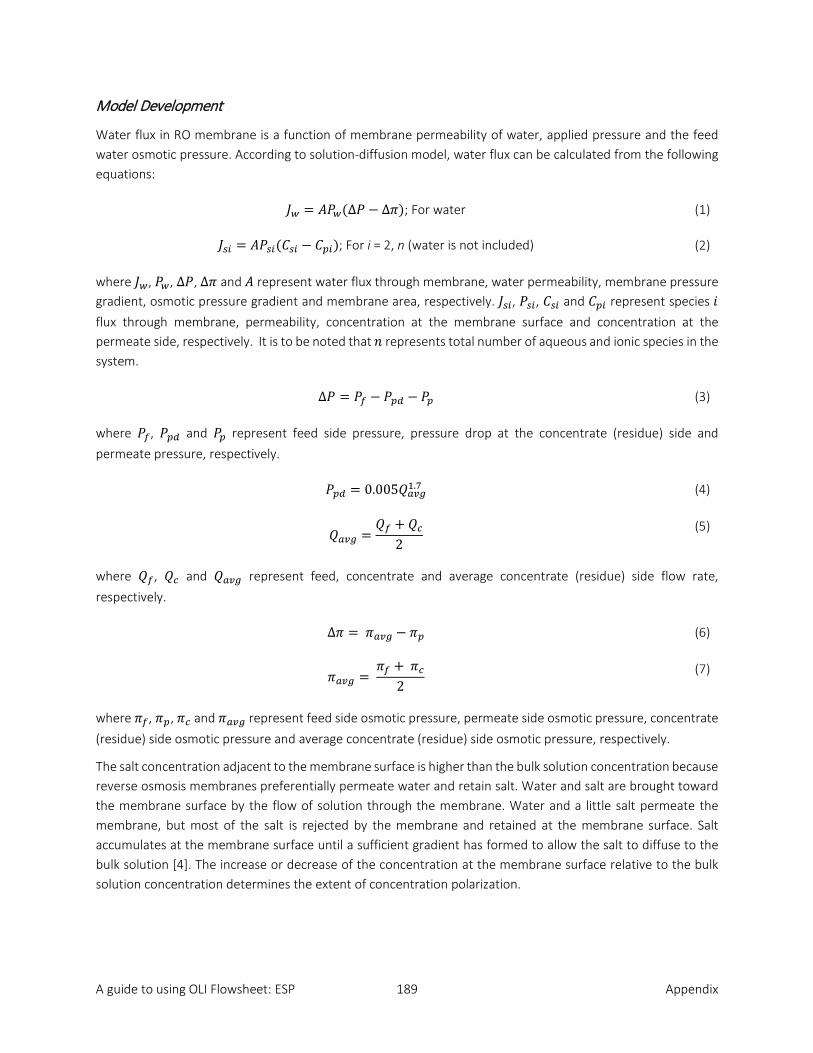
A guide to using OLI Flowsheet: ESP 189 Appendix
Model Development
Water flux in RO membrane is a function of membrane permeability of water, applied pressure and the feed water osmotic pressure. According to solution-diffusion model, water flux can be calculated from the following equations:
𝐽𝐽𝑤𝑤 = 𝐴𝐴𝐴𝐴𝑤𝑤(∆𝐴𝐴 − ∆𝜋𝜋); For water (1)
𝐽𝐽𝑠𝑠𝑖𝑖 = 𝐴𝐴𝐴𝐴𝑠𝑠𝑖𝑖(𝐶𝐶𝑠𝑠𝑖𝑖 − 𝐶𝐶𝑝𝑝𝑖𝑖); For i = 2, n (water is not included) (2)
where 𝐽𝐽𝑤𝑤, 𝐴𝐴𝑤𝑤, ∆𝐴𝐴, ∆𝜋𝜋 and 𝐴𝐴 represent water flux through membrane, water permeability, membrane pressure gradient, osmotic pressure gradient and membrane area, respectively. 𝐽𝐽𝑠𝑠𝑖𝑖, 𝐴𝐴𝑠𝑠𝑖𝑖, 𝐶𝐶𝑠𝑠𝑖𝑖 and 𝐶𝐶𝑝𝑝𝑖𝑖 represent species 𝑖𝑖 flux through membrane, permeability, concentration at the membrane surface and concentration at the permeate side, respectively. It is to be noted that 𝑛𝑛 represents total number of aqueous and ionic species in the system.
∆𝐴𝐴 = 𝐴𝐴𝑓𝑓 − 𝐴𝐴𝑝𝑝𝑝𝑝 − 𝐴𝐴𝑝𝑝 (3)
where 𝐴𝐴𝑓𝑓, 𝐴𝐴𝑝𝑝𝑝𝑝 and 𝐴𝐴𝑝𝑝 represent feed side pressure, pressure drop at the concentrate (residue) side and permeate pressure, respectively.
𝐴𝐴𝑝𝑝𝑝𝑝 = 0.005𝑄𝑄𝑎𝑎𝑎𝑎𝑔𝑔1.7 (4)
𝑄𝑄𝑎𝑎𝑎𝑎𝑔𝑔 =𝑄𝑄𝑓𝑓 + 𝑄𝑄𝑐𝑐
2
(5)
where 𝑄𝑄𝑓𝑓, 𝑄𝑄𝑐𝑐 and 𝑄𝑄𝑎𝑎𝑎𝑎𝑔𝑔 represent feed, concentrate and average concentrate (residue) side flow rate, respectively.
∆𝜋𝜋 = 𝜋𝜋𝑎𝑎𝑎𝑎𝑔𝑔 − 𝜋𝜋𝑝𝑝 (6)
𝜋𝜋𝑎𝑎𝑎𝑎𝑔𝑔 = 𝜋𝜋𝑓𝑓 + 𝜋𝜋𝑐𝑐
2 (7)
where 𝜋𝜋𝑓𝑓, 𝜋𝜋𝑝𝑝, 𝜋𝜋𝑐𝑐 and 𝜋𝜋𝑎𝑎𝑎𝑎𝑔𝑔 represent feed side osmotic pressure, permeate side osmotic pressure, concentrate (residue) side osmotic pressure and average concentrate (residue) side osmotic pressure, respectively.
The salt concentration adjacent to the membrane surface is higher than the bulk solution concentration because reverse osmosis membranes preferentially permeate water and retain salt. Water and salt are brought toward the membrane surface by the flow of solution through the membrane. Water and a little salt permeate the membrane, but most of the salt is rejected by the membrane and retained at the membrane surface. Salt accumulates at the membrane surface until a sufficient gradient has formed to allow the salt to diffuse to the bulk solution [4]. The increase or decrease of the concentration at the membrane surface relative to the bulk solution concentration determines the extent of concentration polarization.

A guide to using OLI Flowsheet: ESP 190 Appendix
𝐶𝐶𝐴𝐴 =𝑅𝑅𝑃𝑃𝐾𝐾
1 + 𝐸𝐸0(𝑅𝑅𝑃𝑃𝐾𝐾 − 1)
(8)
𝐴𝐴𝐾𝐾 = 𝐽𝐽𝑎𝑎𝛿𝛿 𝑑𝑑𝑎𝑎� (9)
where 𝐶𝐶𝐴𝐴, 𝐴𝐴𝐾𝐾, 𝐸𝐸0, 𝐽𝐽𝑎𝑎, 𝛿𝛿 and 𝑑𝑑𝑎𝑎 represent concentration polarization modulus, Peclet number, enrichment factor, typical flux through membrane, boundary layer thickness and typical diffusion coefficient, respectively.
𝐶𝐶𝑠𝑠𝑖𝑖 = 𝐶𝐶𝑝𝑝𝑖𝑖 + 𝐶𝐶𝐴𝐴(𝐶𝐶𝑓𝑓𝑖𝑖 − 𝐶𝐶𝑝𝑝𝑖𝑖) (10)
where 𝐶𝐶𝑠𝑠𝑖𝑖 and 𝐶𝐶𝑓𝑓𝑖𝑖 represent concentration at the membrane surface and feed side bulk concentration for the species, respectively.
The fouling factor is applied to membrane due to loss of permeability by compaction and scale fouling. Typically, a fouling factor less than 1.0 is applied depending on the membrane life. A correlation was developed for fouling factor which considers the water activity reduction at the membrane surface due to permeation relative to the fresh membrane under the test conditions.
𝐹𝐹𝐹𝐹 = 𝑓𝑓𝑣𝑣𝑛𝑛𝑐𝑐𝑅𝑅𝑖𝑖𝑉𝑉𝑛𝑛 (𝑃𝑃𝑐𝑐 ,𝜋𝜋𝑎𝑎𝑎𝑎𝑔𝑔) (11)
where 𝐹𝐹𝐹𝐹, 𝑃𝑃𝑐𝑐 and 𝜋𝜋𝑎𝑎𝑎𝑎𝑔𝑔 represent fouling factor, concentrate (residue) side temperature and average concentrate (residue) side osmotic pressure, respectively.
The osmotic pressure, self-diffusivity and densities are calculated in OLI Systems’ Mixed-Solvent Electrolyte (MSE) or Aqueous (AQ) framework.
Equations (1-11) constitute the solution of the RO membrane and are simultaneously solved to calculate 𝐽𝐽𝑤𝑤, 𝐽𝐽𝑠𝑠𝑖𝑖, 𝐶𝐶𝑝𝑝𝑖𝑖, 𝐶𝐶𝑠𝑠𝑖𝑖, 𝐶𝐶𝐴𝐴 and 𝐹𝐹𝐹𝐹.
Permeability Estimate
In water rich environment, hydration numbers refer to the number of water molecules in the vicinity of the ion. Thus, real radius of an ion is the one that considers the water molecules around it (i.e., the hydrated ion radius) rather than the absolute ionic crystal radius. The water molecules that these hydration number pertain to presumably move together with the ions and are sufficiently firmly attached to them by ion-dipole interactions and hydrogen bonding to constitute a fairly stable entity [6]. Stokes radii are calculated as a function of ionic limiting conductivities and charge of species. The Stokes radii are corrected to relate Van Der Waals ionic sizes [7, 8]. The hydration numbers are calculated as a function of corrected Stokes radii, ionic limiting standard molar volume and molar volume of water. Membrane specific permeation behavior found in open literature were analyzed and from the analyzed data, a correlation was developed for permeability as a function of hydration numbers. It is worth mentioning that regardless of membrane type, the type of experiment, and the membrane configuration, the salt permeabilities are inversely proportional to the hydrated radii of the ions [3]. However, for regressing the water permeability and key components (test solutes) permeabilities, a modified subset of equations (1-11) were formulated and simultaneously solved based on the performance data provided. After calculating water and key components permeabilities, an update (but preserving the trend) in the aforementioned correlation was achieved, and the permeabilities of the rest of the ionic species were calculated from the updated correlation. The advantage of this technique is that a reasonable and preferential order of permeabilities for the membrane regardless of membrane type can be correctly estimated.

A guide to using OLI Flowsheet: ESP 191 Appendix
For some organics with same homologous group (i.e., alcohols, phenols, acids), the rejections were correlated by calculating the topological parameters characterizing molecular structure [5]. For other neutrals, self-diffusivities relative to water were used to correlate the permeability. These calculated permeabilities remain constant unless there is a change in temperature.
References
[1] S.M.J. Zaidi, F. Fadhillah, Z. Khan, and A.F. Ismail. Salt and water transport in reverse osmosis thin film composite seawater desalination membranes. Desalination, 368 (2015) 202. [2] P. Mukherjee, A. Sengupta. Ion exchange selectivity as a surrogate indicator of relative permeability of ions in reverse osmosis processes. Environ. Sci. Technol., 37 (2003) 1432. [3] S.M.S. Ghiu, Mass transfer of ionic species in direct and reverse osmosis processes, Doctoral dissertation, University of South Florida, 2003. [4] R.W. Baker, Membrane technology and applications, 2nd Ed., Chichester, England: Wiley, 2004. [5] A. Ksiązczak, A. Anderko. A chemical approach to the prediction of thermophysical properties of associating compounds. Berichte der Bunsengesellschaft für physikalische Chemie, 92 (1988) 496. [6] Y. Marcus. Ion properties, 1st Ed., New York: Marcel Dekker, 1997. [7] Y. Marcus. Ion solvation, 1st Ed., New York: John Wiley & Sons, 1985. [8] R.E. Nightingale. Phenomenological theory of ion solvation: Effective radii of hydrated ions, J. Phys. Chem., 63 (1959) 1381.
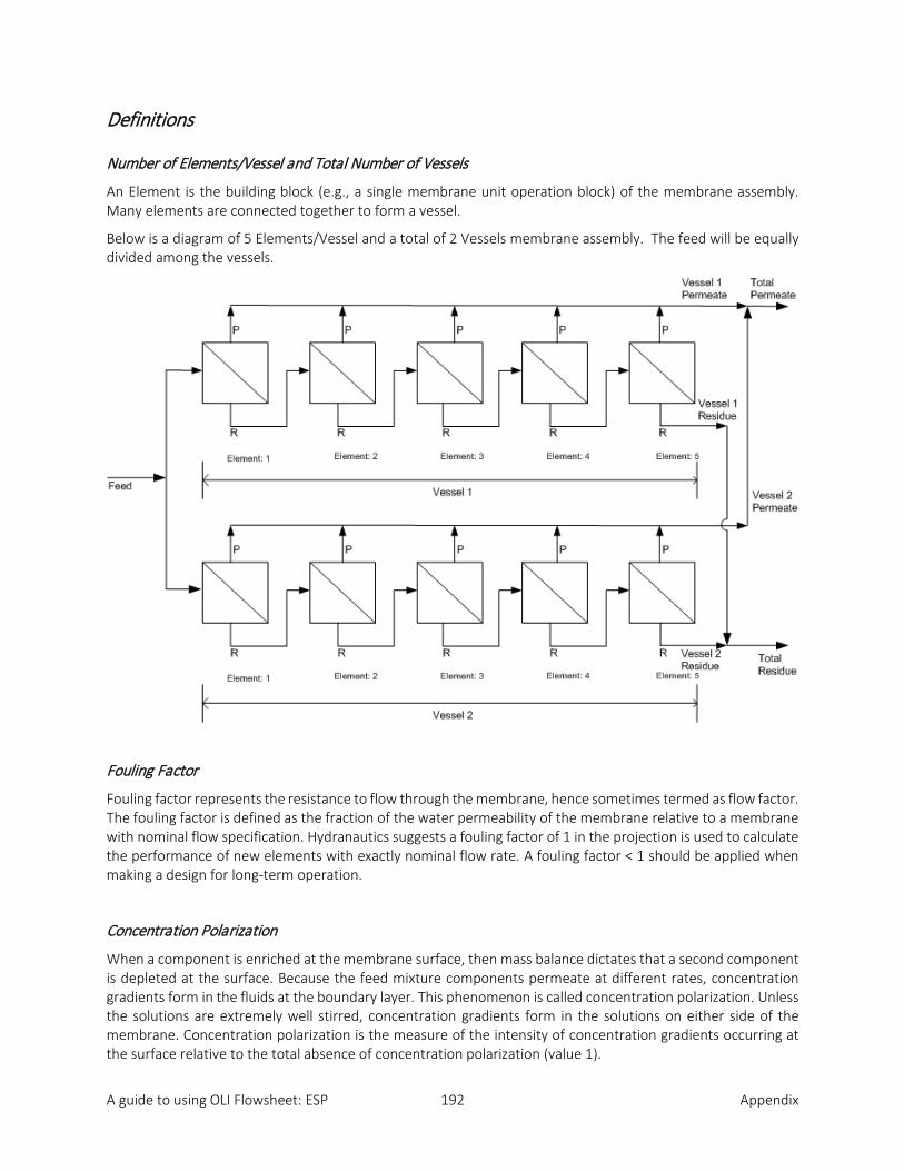
A guide to using OLI Flowsheet: ESP 192 Appendix
Definitions
Number of Elements/Vessel and Total Number of Vessels
An Element is the building block (e.g., a single membrane unit operation block) of the membrane assembly. Many elements are connected together to form a vessel.
Below is a diagram of 5 Elements/Vessel and a total of 2 Vessels membrane assembly. The feed will be equally divided among the vessels.
Fouling Factor
Fouling factor represents the resistance to flow through the membrane, hence sometimes termed as flow factor. The fouling factor is defined as the fraction of the water permeability of the membrane relative to a membrane with nominal flow specification. Hydranautics suggests a fouling factor of 1 in the projection is used to calculate the performance of new elements with exactly nominal flow rate. A fouling factor < 1 should be applied when making a design for long-term operation.
Concentration Polarization
When a component is enriched at the membrane surface, then mass balance dictates that a second component is depleted at the surface. Because the feed mixture components permeate at different rates, concentration gradients form in the fluids at the boundary layer. This phenomenon is called concentration polarization. Unless the solutions are extremely well stirred, concentration gradients form in the solutions on either side of the membrane. Concentration polarization is the measure of the intensity of concentration gradients occurring at the surface relative to the total absence of concentration polarization (value 1).

A guide to using OLI Flowsheet: ESP 193 Appendix
Pressure Drop Per Element
Feed side pressure may reduce during operation resulting in a decrease of the hydraulic pressure difference across membrane. Thus, the feed pressure of the 2nd element (e.g., residue pressure of 1st element) may decrease. Users can either specify the pressure drop per element. In absence of the user specified value, software will calculate the pressure drop.
Control Electroneutrality
Since the permeation rates of the species are different, there could be imbalance of the associated ions. An electroneutrality balance must be achieved on both sides of the membrane. This option controls how the electroneutrality balance will be achieved any time you are out of balance in the solver. By default, it is Cation Control. Currently we follow “Prorate Cations and Prorate Anions” selection as you’ve seen in OLI Studio. Electroneutrality balance by adjusting cations or anions should result in the same flux across membrane.

A guide to using OLI Flowsheet: ESP 194 Appendix
Manufacturer Data Sheet for RO Membranes
Membrane manufactures provide a technical sheet for each type of membrane. In addition to physical dimensions (such as membrane area, spacer arrangement, tube diameter and so on), the technical sheet also reports results of a standard experimental measurement of the membrane, that is, permeate flux, recovery and rejection percentage for NaCl (or other salts) aqueous solution at 25 ⁰C. These are the data we will use to calibrate membrane properties.
The following are standard product sheet information from different manufactures.
Example 1: GE
Example 2: Hydranautics
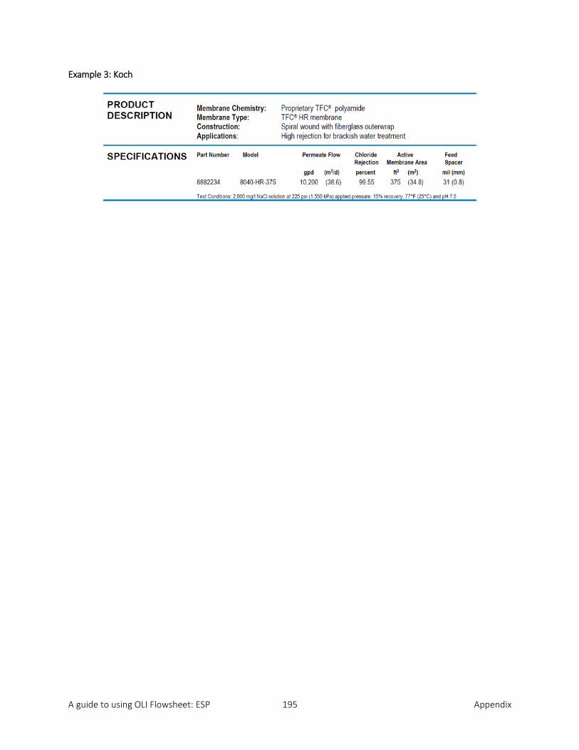
A guide to using OLI Flowsheet: ESP 195 Appendix
Example 3: Koch