A Green Vehicle Routing Problem

Transportation Research Part E 48 (2012) 100–114

Contents lists available at SciVerse ScienceDirect

Transportation Research Part E

journal homepage: www.elsevier .com/locate / t re

A Green Vehicle Routing Problem

Sevgi Erdogan, Elise Miller-Hooks ⇑Department of Civil and Environmental Engineering, University of Maryland, 1173 Glenn L. Martin Hall, College Park, MD 20742, United States

a r t i c l e i n f o a b s t r a c t

Article history:Received 16 December 2010Received in revised form 8 May 2011Accepted 12 July 2011

Keywords:Vehicle routingAlternative-fuel fleet operationsRefuelingFuel tank capacity limitation

1366-5545/$ - see front matter � 2011 Elsevier Ltddoi:10.1016/j.tre.2011.08.001

⇑ Corresponding author. Tel.: +1 301 405 2046; faE-mail addresses: [email protected] (S. Erdoga

A Green Vehicle Routing Problem (G-VRP) is formulated and solution techniques are devel-oped to aid organizations with alternative fuel-powered vehicle fleets in overcoming diffi-culties that exist as a result of limited vehicle driving range in conjunction with limitedrefueling infrastructure. The G-VRP is formulated as a mixed integer linear program. Twoconstruction heuristics, the Modified Clarke and Wright Savings heuristic and the Den-sity-Based Clustering Algorithm, and a customized improvement technique, are developed.Results of numerical experiments show that the heuristics perform well. Moreover, prob-lem feasibility depends on customer and station location configurations. Implications oftechnology adoption on operations are discussed.

� 2011 Elsevier Ltd. All rights reserved.

1. Introduction

In the United States (US), the transportation sector contributes 28% (US EPA, 2009) of national greenhouse gas (GHG)emissions. This is in large part because 97% of US transportation energy comes from petroleum-based fuels (US DOT,2010). Efforts have been made over many decades to attract drivers away from personal automobiles and onto public transitand freight from trucks to rail. Such efforts are aimed at reducing vehicle miles traveled by road and, thus, fossil-fuel usage.Other efforts have focused on introducing cleaner fuels, e.g. ultra low sulfur diesel, and efficient engine technologies, leadingto reduced emissions for the same miles traveled and greater mileage per gallon of fuel used. While each such effort has itsbenefits, only a multi-faceted approach can engender the needed reduction in fossil-fuel usage.

As part of such a multi-faceted approach, renewed attention is being given to efforts to exploit alternative, greener fuelsources, namely, biodiesel, electricity, ethanol, hydrogen, methanol, natural gas (liquid-LNG or compressed-CNG), and pro-pane (US DOE, 2010). Municipalities, government agencies, nonprofit organizations and private companies are convertingtheir fleets of trucks to include Alternative Fuel Vehicles (AFVs), either to reduce their environmental impact voluntarilyor to meet new environmental regulations. This focus on truck conversion is desirable because, while medium- and hea-vy-duty trucks comprise only 4% of the vehicles on the roadways (US FHWA, 2008), they contribute nearly 19.2% of US trans-portation-based GHG emissions (US DOT, 2010). Moreover, truck traffic has had the greatest growth rate of all vehicle traffic,increasing 77% for heavy-duty trucks and 65.6% for light-duty trucks compared with only 3.3% for passenger cars between1990 and 2006 (US DOT, 2010).

The US currently has energy policies in place with the aim of reducing fossil-fuel use so as to reduce GHG emissions, breakdependency on foreign oil, increase homeland security and support renewable energy use (e.g. the Energy Policy Act (EPAct),1992, 2005; Executive Order (EO) 13423 and the Energy Independence and Security Act (EISA), 2007). These policies have ledto the creation of regulations, mandates, tax incentives, etc. that motivate or require companies and agencies to use AFVs. Infact, federal agencies with a fleet of 20 motor vehicles or more are required to reduce petroleum consumption by a minimumof 2% per year through the end of fiscal year 2015 from the 2005 baseline usage. These agencies are required by executive

. All rights reserved.

x: +1 301 405 2585.n), [email protected] (E. Miller-Hooks).

S. Erdogan, E. Miller-Hooks / Transportation Research Part E 48 (2012) 100–114 101

order to increase their alternative fuel use by 10% per year relative to the previous year (EO 13423, 2007). This executiveorder replaced an earlier order (EO 13149, 2000) requiring a 20% reduction in petroleum use by 2005 in comparison to baseyear 1999. The replacement was needed, because no EPAct-covered agency could meet the reduction goal due to insufficientalternative fueling infrastructure. Federal fleets are also required to maximize use of diesel with biodiesel blends (B20) byreplacing medium- and heavy-duty gasoline vehicles with diesel vehicles that can use such biodiesel blends. This require-ment applies to agencies at locations where there is sufficient B20 infrastructure (current or planned). In addition, the USDOE sponsors a program called Clean Cities (US DOE, 2011a) with over 100 local coalitions to support reduction in petroleumuse in the transportation sector.

Agencies consider numerous factors in the selection of a particular vehicle type, including fuel availability and geographicdistribution of fueling stations in the service area, vehicle driving range, vehicle and fuel cost, fuel efficiency, and fleet main-tenance costs. The lack of a national infrastructure for refueling AFVs presents a significant obstacle to alternative fuel tech-nology adoption by companies and agencies seeking to transition from traditional gasoline-powered vehicle fleets to AFVfleets (Melaina and Bremson, 2008). In fact, approximately 98% of the fuel used in the federal government’s 138,000 AFV fleet(of which, 92.8% in 2008 are flex-fuel vehicles that can run on gasoline or ethanol-based E85 fuel) continues to be conven-tional gasoline as a result of a lack of opportunity for refueling using the alternative fuel for which the vehicles were designed(US DOE, 2010). Moreover, existing alternative fueling stations (AFSs) are distributed unevenly across the country and withinspecific regions. Additional operational challenges exist as a result of the reduced driving range of most AFVs.

Similar challenges exist for privately owned AFV fleets as noted in various reports (e.g. Chandler et al., 2000, 2002; USDOE, 1997, 2001, 2006; ATA, 2010). FedEx, in its overseas operations, employs AFVs that run on biodiesel, liquid naturalgas (LNG) or compressed natural gas (CNG). In US operations, hybrid vehicles have dominated, while LPG, biodiesel andCNG use is limited to regions with access to appropriate AFSs (Bohn, 2008).

This paper is concerned with those companies or agencies that employ a fleet of vehicles to serve customers or other enti-ties located over a wide geographical region. Such companies rely on tools to aid in forming low cost tours, so as to savemoney and time resulting from travel to customer locations. These routes typically begin at a depot, visit multiple customersand then return to the depot. The problem of assigning customers to vehicles and ordering the customer visits in formingthese tours is known as the Vehicle Routing Problem (VRP). A variant of the VRP, the Green Vehicle Routing Problem (G-VRP), is introduced herein that accounts for the additional challenges associated with operating a fleet of AFVs.

In this paper, techniques are developed to aid an organization with an AFV fleet in overcoming difficulties that exist as aresult of limited refueling infrastructure. These techniques plan for refueling and incorporate stops at AFSs so as to eliminatethe risk of running out of fuel while maintaining low cost routes. The G-VRP is formulated as a mixed-integer linear program(MILP). Given a complete graph consisting of vertices representing customer locations, AFSs, and a depot, the G-VRP seeks aset of vehicle tours with minimum distance each of which starts at the depot, visits a set of customers within a pre-specifiedtime limit, and returns to the depot without exceeding the vehicle’s driving range that depends on fuel tank capacity. Eachtour may include a stop at one or more AFSs to allow the vehicle to refuel en route.

The G-VRP is illustrated on a simple example problem in Fig. 1. This example involves only one truck with a fuel tankcapacity of Q = 50 gallons and fuel consumption rate of r = 0.2 gallons per mile (or 5 miles per gallon fuel efficiency (Fraeret al., 2005). Three AFSs are available in the region. The vehicle begins its tour at depot D and must visit customers C1–C6 before returning to the depot. To visit these customers, a minimum distance of 339 miles must be traversed. Travel ofsuch a distance would consume 67.8 gallons, 17.8 more gallons of fuel than the vehicle’s tank can hold. Thus, the vehicleneeds to visit at least one AFS in order to serve all customers and return to depot D. The G-VRP takes into account the vehi-cle’s fuel tank capacity limitation and chooses the optimal placement of AFS visits within the tour. Accounting for fuel lim-itations, the optimal solution to the G-VRP involves a stop at one AFS and requires the traversal of 354 miles. Thus, the tourlength is 15 miles longer than the minimum tour length, where fuel tank capacity is assumed to be unlimited.

As the VRP is known to be an NP-hard problem (indicating that the computational effort required for its solution growsexponentially with increasing problem size), and the VRP is a special case of the G-VRP, the G-VRP is NP-hard. Thus, exactsolution of large, real-world problem instances will be difficult to obtain. Two heuristics, the Modified Clarke and Wright

Fig. 1. Illustrative example of a solution to the G-VRP.

102 S. Erdogan, E. Miller-Hooks / Transportation Research Part E 48 (2012) 100–114

Savings (MCWS) heuristic and the Density-Based Clustering Algorithm (DBCA), along with a customized improvement tech-nique, are proposed for solution of such larger problem instances. These techniques are intended to provide decision supportfor a company or agency operating a fleet of AFVs for which limited fueling stations exist. These heuristics provide fast solu-tion capability. Their steps show how the additional problem constraints can be tackled within construction and improve-ment heuristics. Moreover, they provide intuition for the development of more sophisticated implementations. A naturalextension, for example, would be to incorporate the proposed concepts within a tabu search procedure. Numerical experi-ments were designed and conducted to assess heuristic performance as a function of customer location configuration, andstation density and distribution. The techniques are also applied on a hypothetical problem instance meant to replicate amedical textile supplier company’s daily operations in the Washington, DC metropolitan area.

2. Background

A number of works in the literature present optimization-based approaches designed specifically for siting AFSs. Themajority of these works were motivated by the Hydrogen Program that was created during the G.W. Bush administrationand supported by a diverse group of governmental and private sponsors (Nicholas et al., 2004; Kuby and Lim, 2005,2007; Upchurch et al., 2007; Lin et al., 2008a,b; Bapna et al., 2002). Other works focus on military applications and considerissues pertaining to the limited capacity of fuel tanks (e.g. Mehrez et al., 1983; Mehrez and Stern, 1985; Melkman et al.,1986; Yamani et al., 1990; Yuan and Mehrez, 1995). Numerous works address the classical VRP with capacity and distanceconstraints (e.g. Laporte et al., 1985); however, such works do not consider the opportunity to extend a vehicle’s distancelimitation as a consequence of actions taken while en route. Of greater relevance is the multi-depot VRP in which vehiclescan stop at satellite facilities (also referred to as replenishment or inter-depot facilities) to replenish or unload (e.g. Bardet al., 1998; Chan and Baker, 2005; Crevier et al., 2007; Kek et al., 2008; Tarantilis et al., 2008). Such opportunity for reloadingaims to overcome capacity limitations of the vehicles, thus, permitting longer routes and reduced return travel to the centraldepot. In another related work, Ichimori and Hiroaki (1981) addressed a shortest path problem for a single vehicle en routeto a single destination in which stops to refuel are explicitly considered.

It appears that no work in the literature directly addresses the G-VRP or a direct variant thereof. While solution tech-niques developed to address related problems cannot be applied directly in solution of the G-VRP in which fuel tank limitsguide distances that can be traveled, the MILP formulation of the G-VRP developed in the next section builds on conceptsconceived in (Bard et al., 1998). Bard et al. formulated a VRP with Satellite Facilities (VRPSF) problem as an MILP with capac-ity and tour duration limitation constraints. Vehicles with capacity limitations have the option to stop at satellite facilities toreload in order to serve customer demand at the vertices. Subtour elimination constraints that employ time relationships, aswell as concepts used for tracking capacity utilization, employed by Bard et al., are exploited herein.

3. Problem definition and formulation

The G-VRP is defined on an undirected, complete graph G = (V,E), where vertex set V is a combination of the customer setI = {v1, v2, . . . ,vn}, the depot v0, and a set of s P 0 AFSs, F = {vn+1,vn+2, . . . ,vn+s}. The vertex set is V ¼ fv0g [ I [ F ¼fv0;v1;v2; . . . ;vnþsg, |V| = n + s + 1. It is assumed that in addition to the AFSs, the depot can be used as a refueling stationand all refueling stations have unlimited capacities. The set E = {(vi,vj): vi,vj e V, i < j} corresponds to the edges connectingvertices of V. Each edge (vi,vj) is associated with a non-negative travel time tij, cost cij and distance dij. Travel speeds are as-sumed to be constant over a link. In addition, no limit is set on the number of stops that can be made for refueling. Whenrefueling is undertaken, it is assumed that the tank is filled to capacity.

The G-VRP seeks to find at most m tours, one for each vehicle, that starts and ends at the depot, visiting a subset of ver-tices including AFSs when needed such that the total distance traveled is minimized. Vehicle driving range constraints thatare dictated by fuel tank capacity limitations and tour duration constraints meant to restrict tour durations to a pre-specifiedlimit Tmax, apply. It is assumed that all customers can be served by a vehicle that begins its tour at the depot and returns tothe depot after visiting the customer directly within Tmax. Without loss of generality, to reflect real-world service area de-signs, it is assumed that all customers can be visited directly by a vehicle beginning and returning to the depot with at mostone visit to an AFS. This does not preclude the possibility of choosing a tour that serves multiple customers and containsmore than one visit to an AFS.

The formulation distinguishes between visits to AFSs and the depot from customer visits. This is because each AFS may bevisited more than once or not at all. In addition, the depot must be visited at the start and end of each tour and can serve,when desired, as an AFS. Customers, on the other hand, must be visited exactly once. To permit multiple (and possibly zero)visits to a subset of the vertices, while requiring exactly one visit to other vertices, graph G is augmented (to create G0 = (V0,E0)with a set of s0 dummy vertices, U ¼ fvnþsþ1;vnþsþ2; . . . ;vnþsþs0 g, one for each potential visit to an AFS or depot serving as anAFS. V 0 ¼ V [U. Associated with each refueling station v f 2 F is nf dummy vertices for f =0, . . . ,n + s. The number of dummyvertices associated with each AFS, nf, is set to the number of times the associated vf can be visited. nf should be set as small aspossible so as to reduce the network size, but large enough to not restrict multiple beneficial visits. This technique involvingdummy vertices was introduced by Bard et al. (1998) for their application involving stops at intermediate depots for reload-ing vehicles with goods for delivery.


Additional notation used in formulating the G-VRP is defined next.

I0
Set of customer vertices and depot, I0 ¼ fv0g [ I F0 Set of AFS vertices and depot, F0 ¼ fv0g [ F 0, where F 0 ¼ R [U pi Service time at vertex i (if i e I, then pi is the service time at the customer vertex, if i e F, pi is the refueling time at the
AFS vertex, which is assumed to be constant)
r Vehicle fuel consumption rate (gallons per mile) Q Vehicle fuel tank capacity Decision variables xij Binary variable equal to 1 if a vehicle travels from vertex i to j and 0 otherwise yj Fuel level variable specifying the remaining tank fuel level upon arrival to vertex j. It is reset to Q at each refueling
station vertex i and the depot
sj Time variable specifying the time of arrival of a vehicle at vertex j, initialized to zero upon departure from the depot
The mathematical formulation of the G-VRP is as follows:

minX

i;j2V 0

i–j

dijxij ð1Þ

s:t:X

j2V 0

j–i

xij ¼ 1; 8i 2 I ð2Þ

X

j2V 0

j–i

xij 6 1; 8i 2 F0 ð3Þ

X

i2V 0

j–i

xji �X

i2V 0

j–i

xij ¼ 0; 8j 2 V 0 ð4Þ

X

j2V 0nf0g

x0j 6 m ð5Þ

X

j2V 0nf0g

xj0 6 m ð6Þ

sj P si þ ðtij � pjÞxij � Tmaxð1� xijÞ; i 2 V 0;8j 2 V 0 n f0gand i–j ð7Þ0 6 s0 6 Tmax ð8Þt0j 6 sj 6 Tmax � ðtj0 þ pjÞ; 8j 2 V 0 n f0g ð9Þyj 6 yi � r � dijxij þ Qð1� xijÞ; 8j 2 I and i 2 V 0; i–j ð10Þyj ¼ Q ; 8j 2 F0 ð11Þyj P minfr � dj0; r � ðdjl þ dl0Þg; 8j 2 I;8l 2 F 0 ð12Þxi;j 2 f0;1g; 8i; j ð13Þ

The objective (1) seeks to minimize total distance travelled by the AFV fleet in a given day. Constraints (2) ensure thateach customer vertex has exactly one successor: a customer, AFS or depot vertex. Constraints (3) ensure that each AFS(and associated dummy vertices) will have at most one successor vertex: a customer, AFS or depot vertex. Flow conservationis ensured through constraints (4) by which the number of arrivals at a vertex must equal the number of departures for allvertices. Constraints (5) ensure that at most m vehicles are routed out of the depot and constraints (6) ensure that at most mvehicles return to the depot in a given day. A copy of the depot is made to distinguish departure and arrival times at thedepot, which is necessary for tracking the time at each vertex visited and preventing the formation of subtours. The timeof arrival at each vertex by each vehicle is tracked through constraints (7). Constraints (7) along with constraints (8) and(9) make certain that each vehicle returns to the depot no later than Tmax. Constraints (8) specify a departure time fromthe depot of zero (s0 = 0) and an upper bound on arrival times upon return to the depot. Lower and upper bounds on arrivaltimes at customer and AFS vertices given in constraints (9) ensure that each route is completed by Tmax. Constraints (10)track a vehicle’s fuel level based on vertex sequence and type. If vertex j is visited right after vertex i (xij = 1) and vertex iis a customer vertex, the first term in constraints (10) reduces the fuel level upon arrival at vertex j based on the distancetraveled from vertex i and the vehicle’s fuel consumption rate. Time and fuel level tracking constraints, constraints (7)and (10), respectively, serve to eliminate the possibility of subtour formation. Constraints (11) reset the fuel level to Q uponarrival at the depot or an AFS vertex. Constraints (12) guarantee that there will be enough remaining fuel to return to thedepot directly or by way of an AFS from any customer location en route. This constraint seeks to ensure that the vehicleswill not be stranded. One could extend this constraint to permit return paths that visit more than one AFS. These constraintsare implemented through the Java CPLEX interface using if–then logic. Finally, binary integrality is guaranteed through con-straints (13).


The main difficulty in solving any VRP is ensuring that subtours will not be created. In traditional VRP formulations, a setof constraints known as subtour elimination constraints are included. In the G-VRP formulation presented herein, subtoursare prevented through the combination of constraints (7)–(9) acting together.

The formulation of the G-VRP presented in this section builds on the VRPSF formulation by Bard et al. (1998) designed fora delivery routing problem with satellites at which goods can be loaded en route to customers. Similar notation was em-ployed where possible. The G-VRP differs from the VRPSF in several substantial ways. First, the VRPSF does not consider dis-tance restrictions based on fuel tank capacity. As such, the possibility of running out of fuel en route to a customer is notconsidered. Second, fuel is consumed along the network edges, while goods are consumed at the network vertices. Thus,capacity limitations associated with the VRPSF cannot serve in modeling fuel usage limitations. Third, determination ofupper and lower bounds on arrival times at the vertices are complicated by refueling needs. This is because there are manymore combinations of possible vertex sequences than in the VRPSF and the number of AFSs in an instance of the G-VRP willlikely exceed the number of satellite facilities in a typical VRPSF. The additional combinations are due to the fact that in theG-VRP, it is possible that refueling will be required even before arriving at a single customer and travel to a refueling stationmust be considered from every customer en route. This differs from the VRPSF, where reloading at a satellite facility needonly be considered when supplies (i.e. goods) must be replenished. Finally, satellite facilities are strategically located, whilelocations of the AFSs are typically beyond the company’s control, possibly affecting the difficulty associated with determin-ing good routes.

4. Solution of the G-VRP

The vehicle driving range (or fuel tank capacity) limitations and existence of a subset of vertices (the AFSs) that can, butneed not be, visited, as well as the possibility of extending a vehicle’s driving range as a result of a visit to a site along thetour, introduce complications that are not present in classical VRPs or most variants thereof. Thus, heuristics designed for theclassical VRP or related variants cannot be applied directly in solving the G-VRP. Not only might such heuristics result insolutions that perform poorly, but these solutions may not even be feasible. Two heuristics customized for the G-VRP areproposed herein for solution of large problem instances: the MCWS heuristic and DBCA. The Clarke and Wright Savings algo-rithm (Clarke and Wright, 1964) designed for the classical VRP, and customized for its variants, is modified to create theMCWS heuristic so as to tackle the challenges introduced by the G-VRP. The DBCA builds on concepts from the Density BasedSpatial Clustering of Applications with Noise (DBSCAN) algorithm proposed in Ester et al. (1996), for the purpose of discov-ering clusters of arbitrary shapes in large spatial databases, such as satellite images and X-rays. In addition, two tourimprovement techniques involving within-tour edge interchanges and across-tour vertex exchanges designed for the G-VRP that can be applied in series once a tour is constructed are presented herein.

4.1. The MCWS Heuristic

MCWS heuristic

Step 1: Create n back-and-forth vehicle tours (v0–vi–v0), each starting at the depot v0, visiting a customer vertex v i 2 Iand ending at the depot. Add each created tour to the tours list.

Step 2: Calculate the tour duration and distance for all tours in the tours list. Check for feasibility of all initial back-and-forth tours with regard to driving range and tour duration limitation constraints and categorize them as feasible orinfeasible. Place all feasible tours in the feasible tours list and the remainder in the infeasible tour list.

Step 3: For each tour in the infeasible tour list, calculate the cost of an AFS insertion between customer vertices vi and thedepot v0, c(vi,v0) = d(vi,vf) + d(vf,v0) � d(vi,v0) for every AFS ðv f 2 F 0Þ. For every such tour, insert an AFS with the leastinsertion cost. If both driving range and tour duration limitation constraints are met after the insertion of an AFS, addthe resulting tour to the feasible tours list. If the driving range constraint is not met with the addition of any AFS,discard the tour. No starting tour containing more than one AFS is considered.

Step 4: Compute the savings associated with merging each pair of tours in the feasible tours list. To do so, first identify allvertices that are adjacent to the depot in a tour. Create a savings pair list (SPL) that includes all possible pairs of thesevertices (vi,vj) with the condition that each pair is formed by vertices that belong to different tours. Compute thesavings associated with each pair of vertices in the SPL, s(vi,vj) = d(v0,vi) + d(v0,vj) � d(vi,vj), where ððv i;v jÞ 2 I [ F 0Þ.Rank the pairs in the SPL in descending order of savings s(vi,vj).

Step 5:While SPL is not empty

Select and remove the topmost pair of vertices (vi,vj) in the SPL and merge their associated tours.For the selected (vi,vj), check driving range and tour duration limitation constraints.

If both constraints are met, add the resulting tour to the feasible tours list.If the resulting tour duration is less than Tmax, but violates the driving range constraint, compute the insertion

cost c(vi,vj) = d(vi,vf) + d(vf,vj) � d(vi,v0) � d(vj,v0) for savings pair ððv i;v jÞ 2 I [ F 0Þ for every AFS ðv f 2 F 0Þ. Insert the


AFS between vi and vj with the least insertion cost for which the resulting tour is feasible. Check for redundancy: If thetour contains more than one AFS, consider whether it is possible to remove one or more of the AFSs from the tour.Remove any redundant AFSs. Add the resulting tour to the feasible tours list.

If any tour has been added to the feasible tours list, return to Step 4. Otherwise, stop.

The MCWS heuristic terminates with a set of tours that together form a feasible solution to the G-VRP in which con-
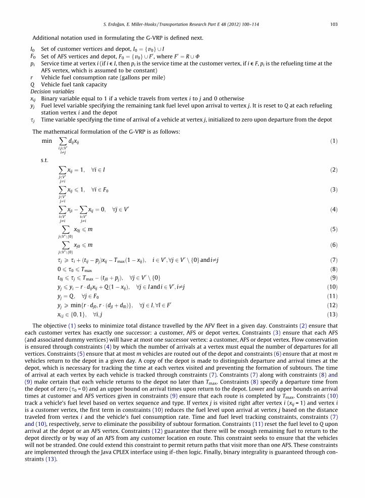
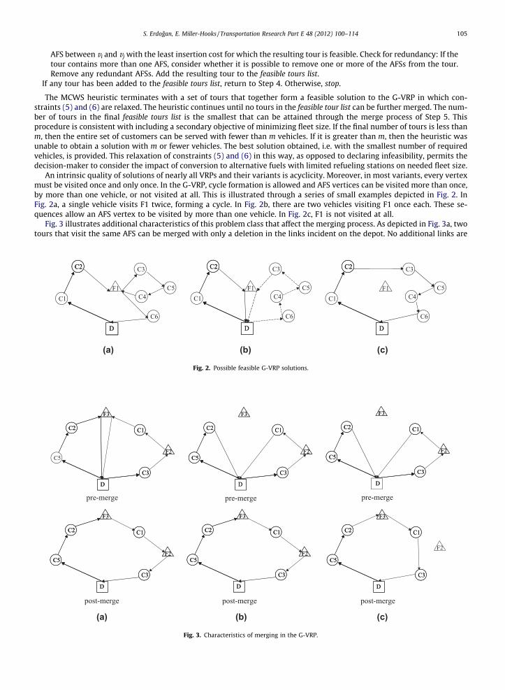
straints (5) and (6) are relaxed. The heuristic continues until no tours in the feasible tour list can be further merged. The num-ber of tours in the final feasible tours list is the smallest that can be attained through the merge process of Step 5. Thisprocedure is consistent with including a secondary objective of minimizing fleet size. If the final number of tours is less thanm, then the entire set of customers can be served with fewer than m vehicles. If it is greater than m, then the heuristic wasunable to obtain a solution with m or fewer vehicles. The best solution obtained, i.e. with the smallest number of requiredvehicles, is provided. This relaxation of constraints (5) and (6) in this way, as opposed to declaring infeasibility, permits thedecision-maker to consider the impact of conversion to alternative fuels with limited refueling stations on needed fleet size.
An intrinsic quality of solutions of nearly all VRPs and their variants is acyclicity. Moreover, in most variants, every vertexmust be visited once and only once. In the G-VRP, cycle formation is allowed and AFS vertices can be visited more than once,by more than one vehicle, or not visited at all. This is illustrated through a series of small examples depicted in Fig. 2. InFig. 2a, a single vehicle visits F1 twice, forming a cycle. In Fig. 2b, there are two vehicles visiting F1 once each. These se-quences allow an AFS vertex to be visited by more than one vehicle. In Fig. 2c, F1 is not visited at all.

Fig. 3 illustrates additional characteristics of this problem class that affect the merging process. As depicted in Fig. 3a, twotours that visit the same AFS can be merged with only a deletion in the links incident on the depot. No additional links are

(a) (b) (c)

Fig. 2. Possible feasible G-VRP solutions.

(a) (b) (c)

Fig. 3. Characteristics of merging in the G-VRP.


required. Moreover, tours that cannot be merged directly may be merged if an AFS is included as depicted in Fig. 3b. When atour containing an AFS is included in a merge that involves an additional AFS visit, as in 3b, it may be that inclusion of an AFSfrom an original tour is redundant. This AFS can be dropped from the final post-merge tour, resulting in, for example, the tourdepicted in Fig. 3c.

4.2. The Density-Based Clustering Algorithm

A second heuristic, the DBCA, is introduced that exploits the spatial properties of the G-VRP. The relative location of cus-tomers and AFSs, as well as their distributions over space, significantly affect feasibility and number of required AFS visits.Like many clustering approaches, the DBCA decomposes the VRP into two clustering and routing subproblems.

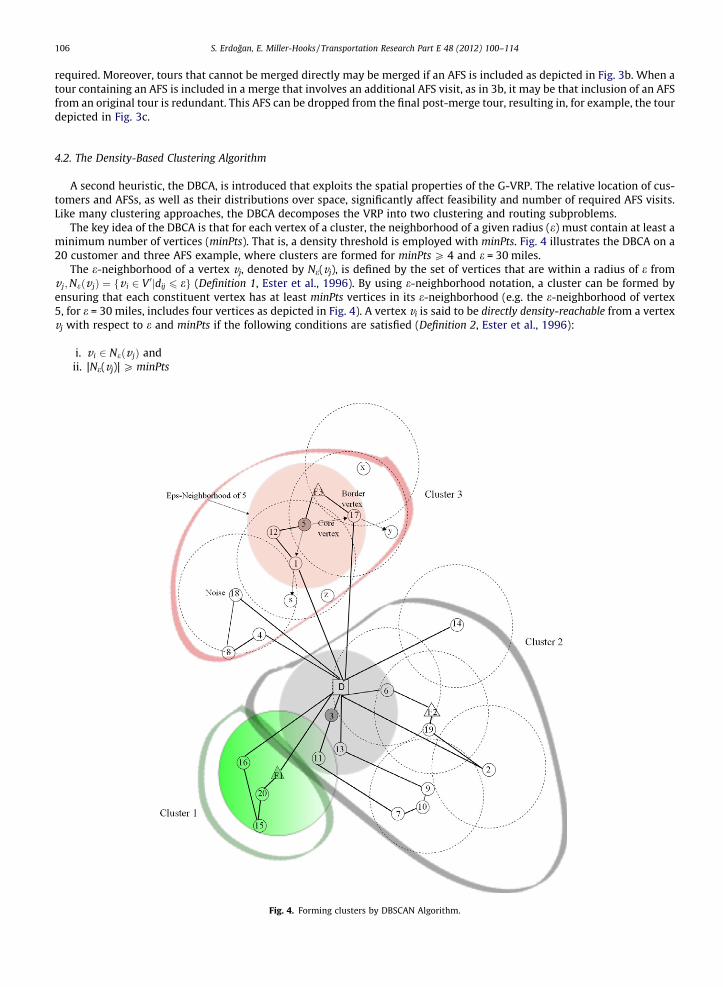
The key idea of the DBCA is that for each vertex of a cluster, the neighborhood of a given radius (e) must contain at least aminimum number of vertices (minPts). That is, a density threshold is employed with minPts. Fig. 4 illustrates the DBCA on a20 customer and three AFS example, where clusters are formed for minPts P 4 and e = 30 miles.

The e-neighborhood of a vertex vj, denoted by Ne(vj), is defined by the set of vertices that are within a radius of e fromv j;Neðv jÞ ¼ fv i 2 V 0jdij 6 eg (Definition 1, Ester et al., 1996). By using e-neighborhood notation, a cluster can be formed byensuring that each constituent vertex has at least minPts vertices in its e-neighborhood (e.g. the e-neighborhood of vertex5, for e = 30 miles, includes four vertices as depicted in Fig. 4). A vertex vi is said to be directly density-reachable from a vertexvj with respect to e and minPts if the following conditions are satisfied (Definition 2, Ester et al., 1996):

i. v i 2 Neðv jÞ andii. |Ne(vj)| P minPts

Fig. 4. Forming clusters by DBSCAN Algorithm.


According to this definition vi is direct-density reachable from vj, but the opposite may not always be true if |Ne(vi)| < min-Pts (i.e. condition (ii) is not met). Condition (ii) is called the core vertex condition. Vertices that do not satisfy this condition arecalled noise vertices. For example, in Fig. 4, vertices 17, F3, 12 and 1 are border vertices, and are directly density reachablefrom vertex 5. However, vertex 5 is not direct-density reachable from any of these vertices. Thus, vertex 5 is a core vertex andis used as a seed to form cluster 3.

A vertex vi is density-reachable from a vertex vm with respect to e and minPts if there is a chain of vertices that satisfy directdensity-reachability for each consecutive vertex pair (Definition 3, Ester et al., 1996). In Fig. 4, vertices y and x are density-reachable from vertex 5 via vertex 17. Density-reachability is a transitive, but not symmetric relation. A vertex vi is density-connected to a vertex vp with respect to e and minPts if there is a vertex vm such that both vi and vp are density reachable fromvm (Definition 4, Ester et al., 1996). For example, vertices y and s are density-connected through vertex 5 in Fig. 4. Using theseconcepts, clusters are formed by identifying sets of density-connected vertices based on a core vertex. Elements of each set areassigned a common cluster ID. In Fig. 4, three core vertices are identified (5, 3 and F1) and three clusters are formed.

Notation used in the DBCA are given next, followed by details of the DBCA.

m
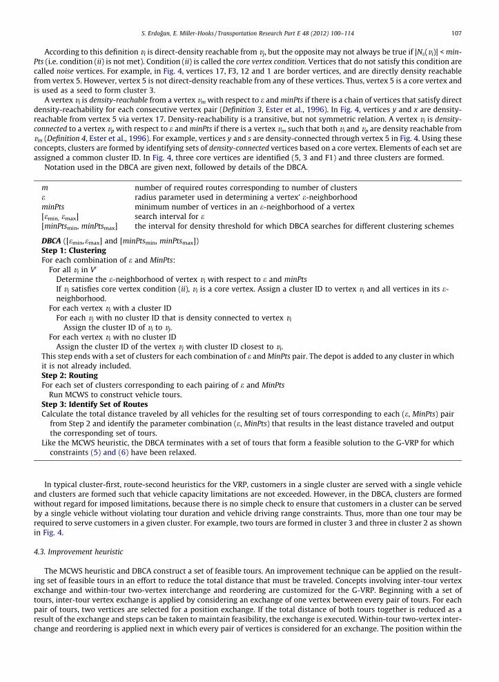
number of required routes corresponding to number of clusters e radius parameter used in determining a vertex’ e-neighborhood minPts minimum number of vertices in an e-neighborhood of a vertex [emin, emax] search interval for e [minPtsmin, minPtsmax] the interval for density threshold for which DBCA searches for different clustering schemes
DBCA ([emin,emax] and [minPtsmin, minPtsmax])Step 1: ClusteringFor each combination of e and MinPts:

For all vi in V0

Determine the e-neighborhood of vertex vi with respect to e and minPtsIf vi satisfies core vertex condition (ii), vi is a core vertex. Assign a cluster ID to vertex vi and all vertices in its e-neighborhood.

For each vertex vi with a cluster IDFor each vj with no cluster ID that is density connected to vertex vi

Assign the cluster ID of vi to vj.For each vertex vi with no cluster ID

Assign the cluster ID of the vertex vj with cluster ID closest to vi.This step ends with a set of clusters for each combination of e and MinPts pair. The depot is added to any cluster in whichit is not already included.Step 2: RoutingFor each set of clusters corresponding to each pairing of e and MinPts

Run MCWS to construct vehicle tours.Step 3: Identify Set of RoutesCalculate the total distance traveled by all vehicles for the resulting set of tours corresponding to each (e, MinPts) pair

from Step 2 and identify the parameter combination (e, MinPts) that results in the least distance traveled and outputthe corresponding set of tours.

Like the MCWS heuristic, the DBCA terminates with a set of tours that form a feasible solution to the G-VRP for whichconstraints (5) and (6) have been relaxed.

In typical cluster-first, route-second heuristics for the VRP, customers in a single cluster are served with a single vehicleand clusters are formed such that vehicle capacity limitations are not exceeded. However, in the DBCA, clusters are formedwithout regard for imposed limitations, because there is no simple check to ensure that customers in a cluster can be servedby a single vehicle without violating tour duration and vehicle driving range constraints. Thus, more than one tour may berequired to serve customers in a given cluster. For example, two tours are formed in cluster 3 and three in cluster 2 as shownin Fig. 4.

4.3. Improvement heuristic

The MCWS heuristic and DBCA construct a set of feasible tours. An improvement technique can be applied on the result-ing set of feasible tours in an effort to reduce the total distance that must be traveled. Concepts involving inter-tour vertexexchange and within-tour two-vertex interchange and reordering are customized for the G-VRP. Beginning with a set oftours, inter-tour vertex exchange is applied by considering an exchange of one vertex between every pair of tours. For eachpair of tours, two vertices are selected for a position exchange. If the total distance of both tours together is reduced as aresult of the exchange and steps can be taken to maintain feasibility, the exchange is executed. Within-tour two-vertex inter-change and reordering is applied next in which every pair of vertices is considered for an exchange. The position within the


tour of the two chosen vertices is exchanged, creating a new tour ordering. If the new tour ordering is infeasible, the ex-change is not performed. Otherwise, if one or both of the chosen vertices for the exchange are AFSs, AFS redundancy ischecked and AFS relocation or exchange with an alternate unscheduled AFS is considered so as to minimize the tour length.The improvement heuristic terminates with a set of tours for the G-VRP for which constraints (5) and (6) have been relaxed.The total distance required to carry out the tours will be no worse than that required of the initial tours to which the pro-cedure is applied.

5. Numerical experiments

Numerical experiments were conducted to assess the quality of solutions obtained through the proposed heuristics onrandomly generated small problem instances through comparison with exact solutions obtained through direct solutionof the G-VRP formulation. The experiments were devised to allow consideration of the impact of customer and AFS locationconfiguration and AFS density on the solution. A larger, more realistic G-VRP was devised using a medical textile supply com-pany’s depot location in Virginia. A customer pool for this company was created based on hospital locations in Virginia (VA),Maryland (MD) and the District of Colombia (DC) using Google Earth. Conversion to biodiesel (B20 or higher) was considered,because of the modest density of biodiesel fueling stations in the region. Such conversion will lead to significant reductionsin carbon monoxide, particulate matter, sulfates, and hydrocarbon as compared with diesel fuel, as well as lifecycle GHGemissions (US EPA, 2002). Actual biodiesel stations located in the region in the summer of 2009 were obtained from a USDOE website (US DOE, 2009). Experiments were designed to analyze the impact of fleet conversion for this company to bio-diesel using the developed heuristics.

In both sets of experiments, unless otherwise stated, a fuel tank capacity of 60 gallons and fuel consumption rate of0.2 gallons per mile were set based on average values for biodiesel-powered AFVs (Fraer et al., 2005). The average vehiclespeed is assumed to be 40 miles per hour (mph) and the total tour duration limitation was assumed to be 11 h. Service timeswere assumed to be 30 min at customer locations and 15 min at AFS locations.

The construction and improvement heuristics were implemented in Java and compiled using Eclipse. Exact solutions wereobtained by implementing the model using ILOG’s CPLEX Concert Technology (version 11.2, 2009) in Java, which allowedJava objects to be used in building the optimization model. The experiments were run on a desktop with Pentium (4)CPU, 32-bit platform with 3.20 GHz processor and 2.00 GB of RAM, while ILOG CPLEX runs were made on a Xeon (R) CPU5160 3.00 GHz processor, 64-bit platform with 16.00 GB of RAM.

5.1. Experiments on small instances

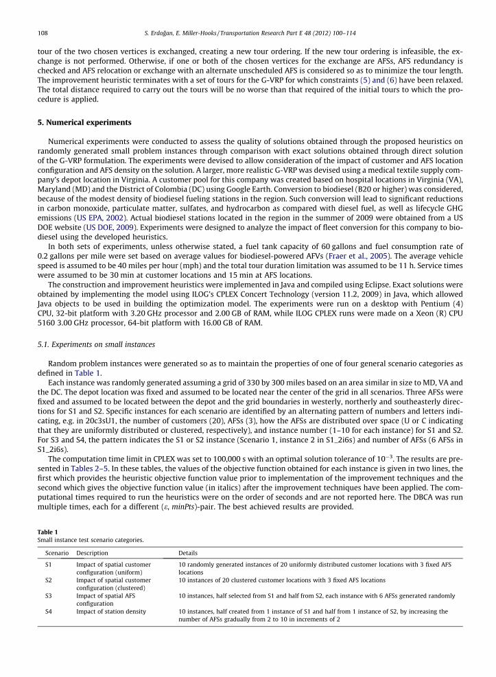
Random problem instances were generated so as to maintain the properties of one of four general scenario categories asdefined in Table 1.

Each instance was randomly generated assuming a grid of 330 by 300 miles based on an area similar in size to MD, VA andthe DC. The depot location was fixed and assumed to be located near the center of the grid in all scenarios. Three AFSs werefixed and assumed to be located between the depot and the grid boundaries in westerly, northerly and southeasterly direc-tions for S1 and S2. Specific instances for each scenario are identified by an alternating pattern of numbers and letters indi-cating, e.g. in 20c3sU1, the number of customers (20), AFSs (3), how the AFSs are distributed over space (U or C indicatingthat they are uniformly distributed or clustered, respectively), and instance number (1–10 for each instance) for S1 and S2.For S3 and S4, the pattern indicates the S1 or S2 instance (Scenario 1, instance 2 in S1_2i6s) and number of AFSs (6 AFSs inS1_2i6s).

The computation time limit in CPLEX was set to 100,000 s with an optimal solution tolerance of 10�3. The results are pre-sented in Tables 2–5. In these tables, the values of the objective function obtained for each instance is given in two lines, thefirst which provides the heuristic objective function value prior to implementation of the improvement techniques and thesecond which gives the objective function value (in italics) after the improvement techniques have been applied. The com-putational times required to run the heuristics were on the order of seconds and are not reported here. The DBCA was runmultiple times, each for a different (e, minPts)-pair. The best achieved results are provided.

Table 1Small instance test scenario categories.

Scenario Description Details

S1 Impact of spatial customerconfiguration (uniform)

10 randomly generated instances of 20 uniformly distributed customer locations with 3 fixed AFSlocations

S2 Impact of spatial customerconfiguration (clustered)

10 instances of 20 clustered customer locations with 3 fixed AFS locations

S3 Impact of spatial AFSconfiguration

10 instances, half selected from S1 and half from S2, each instance with 6 AFSs generated randomly

S4 Impact of station density 10 instances, half created from 1 instance of S1 and half from 1 instance of S2, by increasing thenumber of AFSs gradually from 2 to 10 in increments of 2

Table 2S1, Impact of spatial customer configuration (uniform) results.

Sample CPLEX MCWS DBCA 15 6 e 6 150, 1 6minPts 6 10

Exact solution(miles)

Numberof tours

Customers served Total cost(miles)

Difference (%) Total cost (miles) Difference (%)

20c3sU1 1797.51 6 20 1843.52 2.56 1843.52 2.561818.35 1.16 1797.51 0.00

20c3sU2 1574.82 6 20 1614.15 2.50 1614.14 2.501614.15 2.50 1613.53 2.46

20c3sU3 1765.9 7 20 1969.64 11.54 1969.64 11.251969.64 11.54 1964.57 11.25

20c3sU4 1482.00 5 20 1513.45 2.12 1508.41 1.781508.41 1.78 1487.15 0.35

20c3sU5 1689.35 6 20 1802.93 6.72 1802.93 6.721752.73 3.75 1752.73 3.75a

20c3sU6 1643.05 6 20 1713.39 4.28 1713.39 4.281668.16 1.53 1668.16 1.53a

20c3sU7 1715.13 6 20 1730.45 0.89 1730.45 0.891730.45 0.89 1730.45 0.89

20c3sU8 1709.43 6 20 1766.36 3.33 1766.36 3.331718.67 0.54 1718.67 0.54

20c3sU9 1708.84 6 20 1718.43 0.56 1718.43 0.561714.43 0.33 1714.43 0.33

20c3sU10 1261.15 5 20 1309.52 3.84 1309.52 3.841309.52 3.84 1309.52 3.84

Average 2.79 2.49

a Indicates when a single cluster is formed at the end of the clustering step of DBCA.

Table 3S2, Impact of spatial customer configuration (clustered) results.



Numberof tours

Customersserved

Total cost (miles) Difference (%) Total cost (miles) Difference (%)

20c3sC1 1235.21 5 20 1340.36 8.51 1340.36 8.511300.62 5.30 1300.62 5.30

20c3sC2 1539.94 5 19 1553.53 0.88 1553.53 0.881553.53 0.88 1553.53 0.88a

20c3sC3 985.41 4 12 1083.12 9.92 1083.12 9.921083.12 9.92 1083.12 9.92 a

20c3sC4 1080.16 5 18 1135.90(5) 5.16 1135.90(5) 5.161135.90(5) 5.16 1091.78(4) 1.08

20c3sC5 2190.68 7 19 2190.68 0.00 2190.68 0.002190.68 0.00 2190.68 0.00a

20c3sC6 2785.86 9 17 2887.55 3.65 2887.55 3.652883.71 3.51 2883.71 3.51a

20c3sC7 1393.98 5 6 1703.40 22.20 1703.40 22.201701.40 22.05 1701.40 22.05a

20c3sC8 3319.71 10 18 3319.74 0.00 3319.74 0.003319.74 0.00 3319.74 0.00a

20c3sC9 1799.95 6 19 1811.05 0.62 1811.05 0.621811.05 0.62 1811.05 0.62a

20c3sC10 2583.42 8 15 2667.23 3.24 2667.23 3.242648.84 2.53 2644.11 2.35

Average 5.00 4.57



To ensure that the results are comparable, the heuristics were run and the number of tours required for the best foundsolution was used in constraints (5) and (6) of the formulation in obtaining the corresponding optimal solution. When thetwo heuristics obtained solutions with a different number of tours, as was the case in a few instances, the smaller number oftours was employed in the exact solution. In a number of instances (e.g. S2_4i2s in Table 5), no feasible solution could beobtained. That is, it was not possible to directly visit all customers with one AFS visit, or within the maximum tour duration,requirements of the heuristics. Thus, those customers that could not be served directly with a visit to one AFS or within themaximum tour duration were eliminated from the problem instance. The number of required tours as identified from heu-ristic solutions and final number of customers considered in each instance are provided in the tables.

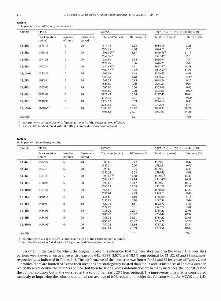
Table 4S3, Impact of spatial AFS configuration results.



Numberof tours

Customersserved


S1_2i6s 1578.15 6 20 1614.15 2.28 1614.15 2.281614.15 2.28 1614.15 2.28

S1_4i6s 1438.89 5 20 1599.56(6) 11.17 1599.56(6) 11.171561.30(6) 8.51 1541.46(5) 7.13

S1_6i6s 1571.28 6 20 1626.94 3.54 1626.94 3.541616.20 2.86 1616.20 2.86

S1_8i6s 1692.34 6 20 1937.87(6) 14.51 1937.87(7) 14.511902.51(6) 12.42 1882.54(6) 11.24

S1_10i6s 1253.32 5 20 1309.52 4.48 1309.52 4.481309.52 4.48 1309.52 4.48a

S2_2i6s 1645.8 6 20 1648.24 0.15 1648.24 0.151645.80 0.00 1645.80 0.00

S2_4i6s 1505.06 6 19 1505.06 0.00 1505.06 0.001505.06 0.00 1505.06 0.00a

S2_6i6s 2842.08 10 20 3127.43 10.04 3127.43 10.043115.10 9.61 3115.10 9.61a

S2_8i6s 2549.98 9 16 2724.12 6.83 2724.12 6.832722.55 6.77 2722.55 6.77

S2_10i6s 1606.65b 6 16 2068.93 28.77 2068.93 28.771995.62 24.21 1995.62 24.21a

Average 5.21 4.93

a Indicates when a single cluster is formed at the end of the clustering step of DBCA.b Best feasible solution found with <11.30% guarantee difference from optimal.

Table 5S4, Impact of station density results.



Numberof tours

Customersserved


S1_4i2s 1582.22 6 20 1589.6 0.47 1589.6 0.471582.2 0.00 1582.2 0.00a

S1_4i4s 1504.1 6 20 1599.6 6.35 1599.6 6.351580.52 5.08 1580.52 5.08a

S1_4i6s 1397.28 5 20 1599.60(6) 14.48 1599.6(6) 14.481561.29(6) 11.74 1541.46(5) 10.32

S1_4i8s 1376.98 6 20 1599.60 16.17 1599.6 16.171561.29 13.39 1561.29 13.39a

S1_4i10s 1397.28 5 20 1568.60 12.26 1568.00 12.221536.04 9.93 1529.73 9.48

S2_4i2s 1080.16 5 18 1135.8 5.16 1135.89 5.161135.89 5.16 1117.32 3.44

S2_4i4s 1466.9 6 19 1522.72 3.81 1522.72 3.811522.72 3.81 1522.72 3.81a

S2_4i6s 1454.96 6 20 1788.22 22.91 1788.22 22.911786.21 22.77 1730.47 18.94

S2_4i8s 1454.96 6 20 1788.22 22.91 1788.22 22.911786.21 22.77 1786.21 22.77

S2_4i10s 1454.93b 6 20 1787.22 22.84 1787.22 22.8420 1783.63 22.59 1729.51 18.87

Average 10.51 9.69

a Indicates when a single cluster is formed at the end of the clustering step of DBCA.b Best feasible solution found with <3.5% guarantee difference from optimal.


It is often in the cases for which the original problem is infeasible that the heuristics perform the worst. The heuristicsperform well, however, on average with a gap of 2.64%, 4.78%, 5.07%, and 10.1% from optimal for S1, S2, S3 and S4 instances,respectively, as indicated in Tables 2–5. The performance of the heuristics was better for S1 and S2 instances of Tables 2 and3 in which there are limited AFSs and their locations are strategically located than for S3 and S4 instances of Tables 4 and 5 inwhich there are double the numbers of AFSs, but their locations were randomly chosen. In many instances, the heuristics findthe optimal solution, but in the worst-case, the solution is nearly 23% from optimal. The improvement heuristics contributedmodestly to improving the solutions obtained (an average of 0.9% reduction in objective function value for MCWS and 1.5%


for DBCA). In closer investigation of the solutions with higher optimality gaps, it was noted that it was often the case thatthese solutions differed from the optimal solution in terms of the number of AFS stations included in the solution tours. Thus,including steps in the improvement procedures that permit changes in the number of AFS stations may produce more sig-nificant improvements.

In general, the results of the two heuristics were very similar; although, whenever there is a difference in solutions ob-tained, the DBCA finds the better solution. This similarity in the obtained solutions may be a consequence of the small size ofthe problem instances. That is, there are few feasible solutions and these techniques often narrow in on the same solutions.Moreover, the heuristics are expected to obtain identical solutions when the DBCA produces a single cluster from the firststage. Those instances in which this arises are noted in Tables 2–5. Out of the 13 instances in which the DBCA produces abetter solution than the MCWS, the DBCA’s solution uses fewer routes to serve the customers in three instances. While therewere differences in the number of AFS visits included in the final tours of all three techniques, no consistent pattern wasnoted. In approximately half the instances, the heuristics employed one fewer or one additional AFS within the final setof tours as compared with the number employed in the optimal set of tours.

The impact of AFS density is examined in S4 (Table 5). Results of these instances indicate that more customers could beserved as the number of AFSs increased. Thus, the number of infeasible instances was reduced. Note that it was not possibleto visit all customers in three of the clustered customer instances (S2_4i6s, S2_8i6s, S2_10i6s) despite the increased numberof AFS options and different location configurations (Table 4). As the number of AFSs increases, the total cost of the optimalsolution decreases for the same number of served customers (Table 5). With a larger number of AFS options, the distancerequired to incorporate needed AFS visits can only decrease. Of course, whether or not an additional AFS will be beneficialdepends on its location.

5.2. Real-world case study

There are 21 publicly available biodiesel stations in VA, MD and DC considered together (US DOE, 2009). Four customer-based scenarios were considered as described in Table 6 in which all 21 AFS locations are considered as options unless other-wise specified.

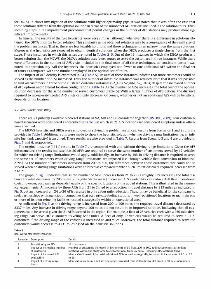
The MCWS heuristic and DBCA were employed in solving the problem instances. Results from Scenarios 1 and 2 runs areprovided in Table 7. Additional runs were made to show the heuristic solution when no driving range limitation (i.e. an infi-nite fuel tank capacity) is assumed. These results are also provided in Table 7. Results from Scenario 3 and 4 are provided inFigs. 5 and 6, respectively.

The original instance (111c) results in Table 7 are compared with and without driving range limitations. Given the AFSinfrastructure, the results indicate that 20 AFVs are required to serve the same number of customers served by 17 vehiclesfor which no driving range limitations would apply. Additionally, an increase by 19% in driving distance is required to servethe same set of customers when driving range limitations are imposed (i.e. through vehicle fleet conversion to biodieselAFVs). As the number of customers increased from 200 to 500, the difference between those customers that could not beserved when no driving range limitations were enforced as compared to when such limitations were required increased from2 to 21.

The graph in Fig. 5 indicates that as the number of AFSs increases from 21 to 28 (a roughly 33% increase), the total dis-tance traveled decreases by 295 miles (a roughly 5% decrease). Increased AFS availability can reduce AFV fleet operationalcosts; however, cost savings depends heavily on the specific locations of the added stations. This is illustrated in the numer-ical experiments. An increase by three AFSs from 21 to 24 led to a reduction in travel distance by 213 miles as indicated inFig. 5, but an increase from 24 to 26 AFSs resulted in only a four mile reduction. Thus, it may be beneficial for the company toseek partnerships with agencies or companies that own private fueling stations in well-positioned locations or maintain oneor more of its own refueling facilities located strategically within an operational area.

As indicated in Fig. 6, as the driving range is increased from 200 to 400 miles, the required travel distance decreased by2337 miles. Any increase in driving range beyond 400 miles did not result in an improved solution, indicating that all cus-tomers could be served given the 21 AFSs located in the region. For example, a fleet of 25 vehicles each with a 250 mile driv-ing range can serve 107 customers traveling 6835 miles. A fleet of only 17 vehicles would be required to serve all 109customers if the driving range of the vehicles is increased to 400 miles. Moreover, the total distance required to serve thecustomers would decrease to 4731 miles based on the heuristic solutions.

Table 6Real world case study scenarios.

Scenario Description Details

1 Transitioning to AFV 111 customers2 Impact of increasing number

of customersNumber of customers increased in increments of 50 from 200 to 500, adding customers at randomlocations within the study area to customer pool from Scenario 1, keeping AFS locations fixed

3 Impact of increased AFSavailability

Identical to Scenario 1, but with additional AFSs located strategically, increased in increments of 2 from 22to 28

4 Impact of driving rangelimits

Identical to Scenario 1, but driving range increased from 200 miles to 500 miles in 50 mile increments

Table 7Heuristic solution results.

Instance Without driving range limit(MCWS)

Modified Clarke and Wright Algorithm(MCWS)

Density Based Clustering Algorithm (DBCA)15 6 e 6 150, 1 6minPts 6 30

Total cost(miles)

Numberof tours

Customersserved

Total cost(miles)

Numberof tours

Customersserved

Total cost(miles)

Numberof tours

Customersserved

111c 4745.90 17 109 5750.62 20 109 5750.62 20 1094731.22 5626.64 5626.64

200c 9358.63 32 196 10617.02 35 190 10617.83 36 191a

9355.56 10428.59 10413.59250c 11691.43 40 244 11965.10 41 235 11965.10 41 236a

11668.388 11886.61 11886.61300c 14782.08 50 293 14331.30 49 281 14331.30 49 282a

14762.41 14242.56 14229.92350c 17677.70 59 343 16610.25 57 329 16610.25 57 329

17661.00 16471.79 16460.30400c 19968.97 67 393 19568.56 67 378 19196.71 66 373

19936.75 19472.10 19099.04450c 23168.02 77 443 21952.48 75 424 21952.48 75 424

21336.91 21854.17 21854.19500c 25032.38 83 492 24652.15 84 471 24652.15 84 471

25024.94 24527.46 24517.08


Fig. 5. Effect of increasing AFSs for instance 111c.

Driving

range

(miles)

Total

Cost

(miles)

Number

of tours

Customers

Served

200 7068.47 28 98

250 6834.97 25 107

300 5626.64 20 109

350 4795.00 17 109

400 4731.22 17 109

500 4731.22 17 109

Fig. 6. Effect of vehicle driving range on total distance traveled.


6. Concluding remarks

In this paper, the G-VRP is formulated and techniques were proposed for its solution. These techniques seek a set of vehi-cle tours that minimize total distance traveled to serve a set of customers while incorporating stops at AFSs in route plans soas to eliminate the risk of running out of fuel. Numerical experiments showed that these techniques perform well compared


to exact solution methods and that they can be used to solve large problem instances. The ability to formulate the G-VRP,along with the solution techniques, will aid organizations with AFV fleets in overcoming difficulties that exist as a resultof limited refueling infrastructure and will allow companies considering conversion to a fleet of AFVs to understand the po-tential impact of their decision on daily operations and costs. These techniques can help companies in evaluating possiblereductions in the number of customers that can be served or increase in fleet size needed to serve an existing customer base,as well as any increase in required distance traveled as a result of driving range limitations and added fueling stops.

The problem posed herein is likely to exist for many years to come. Alternative fuel and vehicle fuel economy legislationdates back to the Clean Air Act (CAA) of 1970. After four decades, limited infrastructure remains a significant barrier to alter-native fuel use adoption in practice. Even today, there are only 7483 AFSs, supporting seven different fuel types in the US (USDOE, 2011b), while there are 161,768 gasoline stations nationwide as of 2007 (US DOE, 2010).

The contributions of this work include: (1) conceptualization of a class of vehicle routing problems involving vehicleswith limited fueling capacity and limited fuel station availability; (2) development and testing of efficient heuristics for solu-tion of large, real-world problem instances, including the specific steps for tracking fuel levels as fuel is consumed andreplenished, and extending a vehicle’s distance limitation by incorporating optional visits to non-unique fueling stationswhile en route; (3) insights into the impact of geographic distribution of stations and customers on operational viability;and (4) a tool to support institutions in reducing their carbon footprint given currently available vehicle technologies andlimited deployment of supporting infrastructure. Thus, concepts proposed herein can be directly applied today and will haveapplicability in future technology adoption as new technologies are introduced nationwide.

The formulation and solution techniques are applicable for any fuel choice. The techniques account for service times atthe stations and, thus, the proposed approach is directly relevant in modeling conversion to electric vehicles in which sig-nificant time may be spent at stations for the purpose of recharging the battery and for possible programs that would permitthe trading of a depleted battery for a fully charged one while en route. Moreover, this approach can be used in seeking opti-mal tours for gasoline or diesel powered fleets that involve special refueling arrangements.

The developed formulation and solution techniques presume that fuel usage is directly related to distance traveled. Themodel could be extended to consider more complex fuel-usage models, consideration of fuel prices and heterogeneous fleetsin which vehicles may have different driving range limitations or be powered by different sources of fuel.

Acknowledgements

This effort was partially funded by the Mid-Atlantic University Transportation Center (MAUTC). This support is gratefullyacknowledged, but implies no endorsement of the findings. The authors are also thankful to Dr. Rahul Nair and Ramzi Mu-khar for their insight and help with implementing the developed techniques.

References

ATA (American Trucking Association), 2010. Is Natural Gas a Viable Alternative to Diesel for the Trucking Industry? White Paper 0610, June 2010. <http://www.truckline.com/AdvIssues/Energy/Natural%20Gas/Natural%20Gas%20Alternative%20-%20White%20Paper%200610.pdf> (accessed 23.04.11).

Bapna, R., Thakur, L.S., Nair, S.K., 2002. Infrastructure development for conversion to environmentally friendly fuel. European Journal of OperationalResearch 1423, 480–496.

Bard, J., Huang, L., Dror, M., Jaillet, P., 1998. A branch and cut algorithm for the VRP with satellite facilities. IIE Transactions 30, 821–834.Bohn, J., 2008. FedEx Implements Green Fleet Initiative. <http://www.worktruckonline.com/Channel/Fuel-Management/Article/Story/2008/09/FedEx-

Implements-Green-Fleet-Initiative.aspx> (accessed 15.09.10).Chan, Y., Baker, S.F., 2005. The multiple depot, multiple traveling salesmen facility-location problem: vehicle range, service frequency and heuristic

implementations. Mathematical and Computer Modeling 41, 1035–1053.Chandler, K., Norton, P., Clark, N., 2000. Raley’s LNG Truck Fleet: Final Results. Alternative Fuel Truck Evaluation Project, Prepared by DOE/NREL.Chandler, K., Walkowicz, K., Clark, N., 2002. UPS CNG Truck Fleet Results: Final Results. Alternative Fuel Truck Evaluation Project, Prepared by DOE/NREL.Clarke, G., Wright, J.W., 1964. Scheduling of vehicle from central depot to a number of delivery points. Operations Research 12, 568–581.Crevier, B., Cordeau, J-F., Laporte, G., 2007. The multi-depot vehicle routing problem with inter-depot routes. European Journal of Operational Research 176,

756–773.EISA (the Energy Independence and Security Act), 2007. Public Law 110-140, December 19, 2007.EPAct (The Energy Policy Act), 1992. Public Law 102-486, October 24, 1992.Executive Order (EO) 13149, 2000. Greening the Government through Federal Fleet and Transportation Efficiency. Federal Register, vol. 65, No. 81,

Wednesday, April 26, 2000.Executive Order (EO) 13423, 2007. Strengthening Federal Environmental, Energy, and Transportation Management. Federal Register, vol. 72, No. 17, Friday,

January 26, 2007.EPAct (The Energy Policy Act), 2005. Public Law 109-58, August 8, 2005.Ester, M., Kriegel, H.P., Sander, J., Xu, X., 1996. A density-based algorithm for discovering clusters in large spatial databases. In: Proceedings of the

International Conference on Knowledge Discovery and Data Mining (KDD.96), Portland, Oregon, pp. 226–231.Fraer, R., Dinh, H., Kenneth, P., Robert, L., McCormick, C.K., 2005. Operating Experience and Teardown Analysis for Engines Operated on Bio-diesel Blends

(B20). SAE Technical Paper No. 2005-01-3641.Ichimori, T., Hiroaki, I., 1981. Routing a vehicle with the limitation of fuel. Journal of the Operations Research Society of Japan 24 (3), 277–281.Kek, A.G.H., Cheu, R.L., Meng, Q., 2008. Distance-constrained capacitated vehicle routing problems with flexible assignment of start and end depots.

Mathematical and Computer Modelling 47, 140–152.Kuby, M., Lim, S., 2005. The flow-refueling location problem for alternative-fuel vehicles. Socio-Economic Planning Science 39, 125–145.Kuby, M., Lim, S., 2007. Location of alternative-fuel stations using the flow-refueling location model and dispersion of candidate sites on arcs. Networks and

Spatial Economics 7, 129–152.Laporte, G., Nobert, Y., Desrochers, M., 1985. Optimal routing under capacity and distance restrictions. Operations Research 33 (5), 1050–1073.Lin, Z., Ogden, J., Fan, Y., Chena, C.-W., 2008a. The fuel-travel-back approach to hydrogen station siting. International Journal of Hydrogen Energy 33 (12),

3096–3101.


Lin, Z., Chena, C.-W., Ogden, J., Fan, Y., 2008b. The least cost hydrogen for southern California. International Journal of Hydrogen Energy 33 (12), 3009–3014.Mehrez, A., Stern, H.I., 1985. Optimal refueling strategies for a mixed-vehicle fleet. Naval Research Logistics Quarterly 32, 315–328.Mehrez, A., Stern, H.J., Ronen, D., 1983. Vehicle fleet refueling strategies to maximize operational range. Naval Research Logistics Quarterly 30, 319–342.Melaina, M.W., Bremson, J., 2008. Refueling availability for alternative fuel vehicle markets: sufficient urban station coverage. Energy Policy 36 (8), 3223–

3231.Melkman, A., Stern, H.I., Mehrez, A., 1986. Optimal refueling sequence for a mixed fleet with limited refuelings. Naval Research Logistics Quarterly 33, 759–

762.Nicholas, M., Handy, S., Sperling, D., 2004. Using geographic information systems to evaluate siting and networks of hydrogen stations. Transportation

Research Record 1880, 126–134.Tarantilis, C.D., Zachariadis, E.E., Kiranoudis, C.T., 2008. A hybrid guided local search for the vehicle-routing problem with intermediate replenishment

facilities. INFORMS Journal on Computing 20 (1), 154–168.Upchurch, C., Kuby, M., Lim., S., 2007. A capacitated model for location of alternative-fuel stations. Geographical Analysis 41 (1), 85–106.US DOE, Department of Energy, 1997. Running Line-Haul Trucks on Ethanol: The Archer Daniels Midland Experience. Prepared and Originally Published by

the Center for Transportation Technologies at the National Renewable Energy Laboratory.US DOE, Department of Energy, 2001. UPS CNG Truck Fleet Start-Up Experience. Alternative Fuel Truck Evaluation Project, Prepared by DOE/NREL.US DOE, Department of Energy, 2006. Federal Fleet Compliance with EPACT and EO 13149, Fiscal Year 2006. <http://www.afdc.energy.gov/afdc/pdfs/

ff22_federal_fleet_report.pdf> (accessed 20.11.10).US DOE, Department of Energy, 2009.The Alternative Fuels and Advanced Vehicles Data Center (AFDC). <http://www.afdc.energy.gov/afdc/locator/stations/

state> (accessed 24.06.09).US DOE, Department of Energy, 2010. Transportation Data Book, Edition 29 by Davis, S.C., Diegel, S.W., Boundy, R.G. Oak Ridge National Laboratory, ORNL-

6985.US DOE, Department of Energy, 2011a. What is Clean Cities? Brochure prepared by the National Renewable Energy Laboratory (NREL), the US DOE, Office of

Energy Efficiency and Renewable Energy, DOE/GO-102011-3309, May 2011.US DOE, Department of Energy, 2011b. The Alternative Fuels and Advanced Vehicles Data Center (AFDC). <http://www.afdc.energy.gov/afdc/fuels/

stations_counts.html> (accessed 28.04.11).US DOT, Department of Transportation, 2010. The Transportation’s Role in Reducing US Greenhouse Gas Emissions. <http://ntl.bts.gov/lib/32000/32700/

32779/DOT_Climate_Change_Report_-_April_2010_-_Volume_1_and_2.pdf> (accessed 10.11.10).US EPA, Environmental Protection Agency, 2002. A Comprehensive Analysis of Biodiesel Impacts on Exhaust Emissions. Draft Technical Report, EPA420-P-

02-001.US EPA, Environmental Protection Agency, 2009. Inventory of US Greenhouse Gas Emissions and Sinks: 1990–2007, EPA 430-R-09-004.US FHWA, Federal Highway Administration, 2008. Highway Statistics 2008. <http://www.fhwa.dot.gov/policyinformation/statistics/2008/vm1.cfm>

(accessed 21.10.10).Yamani, A., Hodgson, T.J., Martin-Vega, L.A., 1990. Single aircraft mid-air refueling using spherical distances. Operations Research 38 (5), 792–800.Yuan, Y., Mehrez, A., 1995. Refueling strategies to maximize the operational range of a nonidentical vehicle fleet. European Journal of Operational Research

83 (1), 167–181.

A Green Vehicle Routing Problem

Documents

Transcript of A Green Vehicle Routing Problem