Simulated annealing algorithm for vehicle routing problem ...

Ref. code: 25595722040291ANJRef. code: 25595722040291ANJ

SIMULATED ANNEALING ALGORITHM FOR

VEHICLE ROUTING PROBLEM WITH

TRANSSHIPMENT

BY

SUKANYA THONETHONG

A THESIS SUBMITTED IN PARTIAL FULFILLMENT OF

THE REQUIREMENTS FOR THE DEGREE OF MASTER OF

ENGINEERING (LOGISTICS AND SUPPLY CHAIN SYSTEMS

ENGINEERING)

SIRINDHORN INTERNATIONAL INSTITUTE OF TECHNOLOGY

THAMMASAT UNIVERSITY

ACADEMIC YEAR 2016


ii

Acknowledgements

First and foremost, I would like to express my sincere gratefulness to my

advisor Assoc. Prof. Dr. Jirachai Buddhakulsomsiri for his patience, motivation, and

enormous knowledge of my research. He give me not only advices on my research but

also continuing encouragement, kind support, and guiding me with full dedication

throughout my study. This research would not be accomplished without him. I would

like to thank all my committee members, Asst. Prof. Dr. Narameth Nananukul, Assoc.

and Prof. Dr. Huynh Trung Luong for their helpful comments and valuable suggestions.

Their advice have always been helpful to my study.

Last but not least, this acknowledgement would be incomplete without

expressing to my family members, especially my parents for continuously supporting

and encouraging throughout my life.


iii

Abstract

SIMULATED ANNEALING ALGORITHM FOR VEHICLE ROUTING

PROBLEM WITH TRANSSHIPMENT

by

SUKANYA THONETHONG

Bachelor of Engineering. (Industrial Engineering) Naresuan University, 2012.

Master of Engineering. (Logistics and Supply Chain Systems Engineering),

Sirindhorn International Institute of Technology, 2016.

A vehicle routing problem (VRP) involves a problem of determining

transportation routes for a fleet of vehicles that exist to provide delivery services from

a depot to satisfy a set of geographically dispersed customers’ demands. The vehicle

routing problem with transshipment (VRPT) defined in this study is the VRP that

includes transshipment demand between pairs of customers, in addition to the regular

demand. Transshipment demands are demands for seasonal product that change model

or design every season such that the depot can only place a one-time order for the item

before the selling season. At the middle towards the end of a selling season, inventories

of the item are already distributed to all the retail stores, i.e. the depot no longer has the

item. As end customer demands for the item arrive at a retail store that already sold out

the item, one way to satisfy the end customer demand is to transship the from another

retail store that still has the item. Motivation for the VRPT is from a real world problem

found in one of the largest retail chains in Thailand. The current practice at the depot

of this retail chain is that when transshipment demand is requested, a delivery vehicle

will pick-up the item from one retail store, bring it back to the depot and store it, then

deliver to the retail store that request the item in the next delivery trip. In order to

improve customer service by reducing the delivery time of transshipment demand, the

objective is to determine delivery routes for vehicles that can pick up the item at one

store and deliver it to another store on the same trip. In other words, the pick-up and

drop-off of transshipment demand must be performed in addition to the delivery of


iv

regular demand from the depot to the retail stores by the same vehicle. A simulated

annealing (SA) algorithm is developed to generate delivery routes in which both

demands can be satisfied in the same delivery routes while minimizing the

transportation cost. The algorithm was tested with standard problem instances of

capacitated vehicle routing (CVRP). The results from testing the algorithm using

numerical examples shows that there is a tradeoff between additional cost of allowing

delivery of transshipment demands on the same trip and the benefit of reducing delivery

lead time of transshipment demand.

Keywords: Vehicle Routing Problem; Transshipment; Simulated Annealing


Table of Contents

Chapter Title Page

Signature Page i

Acknowledgements ii

Abstract iii

Table of Contents v

List of Figures vi

List of Tables vii

1 Introduction 1

1.1 Problem Statement 1

1.2 Research Objectives 3

1.3 Research Overview 3

2 Literature Review 4

2.1 Vehicle Routing Problems 4

2.1.1 Capacitated VRP 4

2.1.2 VRP with backhauls 5

2.1.3 VRP with pick-up and delivery 5

2.1.4 VRP with time windows 6

2.1.5 Stochastic VRP 7

2.2 Solution Techniques for VRP 7

2.3 Vehicle Routing Problem featuring Transshipment 7

3 Methodology 9

3.1 Method of Approach 9

3.2 Simulated Annealing Algorithm 10


vi

3.2.1 Algorithm Parameter Tuning 11

3.3 Vehicle Routing Problem with Transshipment (VRPT) 13

3.4 Numerical Example 14

3.4.1 Problem Instance 14

3.4.2 Results and Discussion 17

4 Computational Experiment, Result and Discussion 18

4.1 Test Problems 18

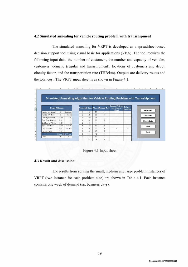
4.2 Simulated annealing for vehicle routing problem with transshipment

19

4.3 Result and discussion 19

5 Conclusions 22

References 23

Appendices 26

Appendix A 27


vii

List of Figures

Figures Page

3.1 Method of approach diagram 9

3.2 An illustration of the VRPT 14

3.3 The VRPT solution representation 14

4.1 Input sheet 19


viii

List of Tables

Tables Page

3.1 Comparison of results for instance set A ............................................ 12

3.2 Locations and a set of regular demand ................................................ 16

3.3 Transshipment demand ....................................................................... 16

3.4 Test result on 1, 2, and 3 transshipment demand ................................ 17

4.1 Test results .......................................................................................... 20

A.1 Locations and a set of regular demand for S1 and S2 problem 28

A.2 Transshipment demand for S1 problem ............................................. 29

A.3 Transshipment demand for S2 problem ............................................. 29

A.4 Locations and a set of regular demand for M1 and M2 problem ....... 30

A.5 Transshipment demand for M1 problem ............................................ 33

A.6 Transshipment demand for M2 problem ............................................ 34

A.7 Locations and a set of regular demand for M1 and M2 problem ....... 35

A.8 Transshipment demand for L1 problem ...................................... 39

A.9 Transshipment demand for L2 problem ............................................. 40


1

Chapter 1

Introduction

Dantzig and Ramser (1959) firstly introduced the Vehicle Routing Problem

(VRP). The problem was modelled after a routing optimization problem for petrol

deliveries by truck. The objective is to find the optimal set of routes for a fleet of

vehicles to perform delivery services to a set of customers so as to minimize the total

transportation cost. Since then, numerous research studies have been conducted to solve

the VRP using exact and heuristics algorithms. There are also many variants of the

VRP, such as VRP with time windows (VRPTW), VRP with pickup and delivery

(VRPPD), etc.

1.1 Problem Statement

This study presents one of the variants of vehicle routing problem (VRP),

so-called, vehicle routing problem with transshipment (VRPT) in this study. Customer

demands are of two types: regular demands that can be satisfied by inventories at the

depot and transshipment demands that request of items from other customers. The

motivation for the VRPT is from a real world problem found in one of the largest retail

chains in Thailand. In this problem, a depot exists to satisfy daily demand from many

retail stores, all of which are in the same retail chain under a single ownership. The

retail chain offers products that are both continuously stocked and seasonal products.

The focus is on seasonal products, which are usually ordered once a year from both

domestics and international suppliers. These items arrive before the beginning of the

selling season, and are kept at the depot, and the retail stores would order these items

according to the store’s projected sale figure.

By the middle of a season, all inventories of a seasonal item would be

ordered and kept at the retail stores, and the depot would no longer have inventory of

the item available. At this point, there are many occurrences when demands from end

customers arise at a retail store that already has the items sold out, while the desired

items are available at some other retail stores. The current practice of the company is


2

as follows: (1) The store, so-called delivery customer, that needs the items would issue

a request to the depot. (2) Delivery truck that visits another store that has the item, so-

called pick-up customer, would pick up the item and bring it back to the depot. (3) The

depot then sends the item to the delivery store in the next delivery cycle. The process

usually takes at least as long as the length of the delivery cycle. For example, the process

takes at least one day if the deliveries to both the pick-up and delivery stores are

performed on a daily basis, or it takes at least two days, if delivery cycle is on alternate

day basis.

The company is considering changing this process in order to satisfy the

end customer demand in a shorter time. Specifically, the depot would like to design

delivery routes that take into account the pick-up / delivery demands between stores,

which is called transshipment demand in this study. The delivery routes that can satisfy

the transshipment demand in addition to the regular demand from the depot must have

the truck visits the pick-up store prior to the delivery store on the same route. In other

words, the pick-up item from one store will be delivered to another store on the same

trip. Benefit from the same day delivery would give the retail stores a significant

advantage in terms of customer service in the highly competitive retail business

environment. The company would like to incorporate this change without having to

incur too much additional delivery cost.

This study presents an algorithm development for the VRPT that can

generate good routing solution that allows both regular demand and transshipment

demand deliveries on the same trip. The objective function is to minimize the total

transportation cost. The algorithm is based on the well-known simulated annealing (SA)

algorithm with solution generation mechanism that forces transshipment delivery.

Specifically, the VRPT under study has the following characteristics:

1. There is one central depot.

2. There are many retails stores (customers), each of which may have up to

two types of demand: regular demand that must be satisfied directly by the

depot, and transshipment demand that can only be satisfied from inventory

at another customer.

3. Trucks are of the same type and have the same limited capacity.


3

4. All trips start at the depot and must return to the depot after the end of the

trips.

5. Distance (or travel time) from one node (i.e. depot or retail stores) to

another node is assumed known and constant.

1.2 Research Objectives

The objectives for this study can be stated as follows:

To develop and efficient simulated annealing (SA) algorithm for the Vehicle

Routing Problem with Transshipment (VRPT) under study.

To test the algorithm on problem instances of the VRPT to gain some

fundamental insights on satisfying transshipment demand.

1.3 Research Overview

The remainder of this thesis is organized as follows. Chapter 2 provides a

literature review, including VRP, solution techniques, and related problem to VRPT.

The developed methodology is described in Chapter 3, which includes the VRPT,

simulated annealing (SA) and a numerical example. Then, in Chapter 4 computational

experiment, analysis results and discussion are presented. Finally, conclusion and

recommendations are given in Chapter 5.


4

CHAPTER 2

LITERATURE REVIEW

This chapter contains the literature review of previous research related to

this thesis’s topic. Firstly, an overview of the vehicle routing problem (VRP) is

provided, followed by reviews of the solution techniques available for VRP. Finally,

the literature review of related research studies to the vehicle routing problem with

transshipment.

2.1 Vehicle Routing Problems

The Vehicle Routing Problem was first introduced by Dantzig & Ramser

(1959). The problem was modelled after a routing optimization problem for petrol

deliveries by truck. The objective is to find the optimal set of routes for a fleet of

vehicles to perform deliver services to a set of customers so as to minimize the total

transportation cost. Since then, numerous research studies have been conducted to solve

the VRP using exact and heuristics algorithms. There are also many variants of the

VRP, such as the capacitated VRP (CVRP), VRP with time window (VRPTW), VRP

with backhaul (VRPB), VRP with pickup and delivery (VRPPD), and stochastic VRP

(SVRP). Due to the vast literature review on VRP, each variant of VRP will be briefly

described, and followed by recent research studies of the problem.

2.1.1 Capacitated VRP

The capacitated vehicle routing problem (CVRP) is a VRP in which a

homogenous fleet of delivery vehicles with the same capacity must provide delivery

service to known customer demands. The objective is to minimize the total cost, while

the total demands delivered in each trip cannot exceed vehicle’s capacity.

Recent studies in CVRP by using heuristic and metaheuristic are from W.Y.

et al. (2011), Yiyong et al. (2012), Jianyong et al. (2014), Kenneth and Patrick (2013),

and Yiyong et al. (2014). W.Y. et al. (2011) proposed enhanced version of the artificial

bee colony heuristic. Yiyong et al. (2012) developed a mathematical optimization

model, and proposed SA algorithm with a hybrid exchange rule to solve CVRP and the


5

FCVRP. Kenneth and Patrick (2013) developed an intelligent path relinking procedure

based on the relocate distance. Jianyong et al. (2014) proposed a cooperative parallel

metaheuristic, which consists of multiple parallel tabu search threads. Yiyong et al.

(2014) presented the variable neighbourhood simulated annealing (VNSA) algorithm,

which combined VNS with SA.

2.1.2 VRP with backhauls

Vehicle routing problem with backhauls (VRPB) is a VRP that considers

both delivery of items from the depot (line-haul) and pickup of items back to the depot

(backhaul). VRPB assumes that all deliveries must be made on the route before pickups

can be performed.

Recent studies on VRPB are from Ismail and Fulya (2015), Ilker and Nursel

(2015), and Daniel et al. (2014). Ismail and Fulya (2015) proposed a memetic algorithm

to solve the Capacitated Location-Routing Problem with Mixed Backhauls (CLRPMB),

which finds locations of the depots and designs route that pickup and delivery demands

of each customer must be served with the same vehicle. Ilker and Nursel (2015)

presented an advanced algorithm to solve the VRP with backhauls and time windows

(VRPBTW) that includes capacity, backhaul and time window constraints, is a hybrid

meta-heuristic algorithm (HMA). The objective is to minimize the total distance.

Lastly, Daniel et al. (2014) proposed a simple iterated local search algorithm for the

VRPB.

2.1.3 VRP with pick-up and delivery

Vehicle routing problem with pickup and delivery (VRPPD, sometimes

denoted as PDP) is an extension of VRPB. Pure pickup or delivery only performs

pickup or delivery in the routes. Mixed pickup and delivery has two types: (1) a route

is not interspersed, which means the vehicle must finish all delivery demands before

performing the pick-up on the same route, and (2) interspersed route that mixes pickup

and delivery on the same route. Another variant of the VRPPD is the VRP with

simultaneous pick-up and delivery (VRPSPD), where delivery and pickup demands are

required to be made simultaneously at each customer stop.

Recent studies on VRPPD are from Tajik et al. (2014), who proposed a new

mixed integer linear programming (MILP) for a new time window pickup-delivery


6

pollution routing problem (TWPDPRP) to manage with unsteady input data. Mustafa

and Qingfeng et al. (2014) developed an easy-to-implement heuristic for the routing

problem with unpaired pickup and delivery with split loads. Mustafa and Seyda (2015)

developed an adaptable local search solution method, which a SA inspired algorithm

with Variable Neighborhood Descent for both the VRP with Mixed Pickup and

Delivery (VRPMPD) and the VRP with Simultaneous Pickup and Delivery (VRPSPD),

which are different in that the customers may have pickup or delivery demand. Olcay

et al. (2015) proposed a mixed-integer mathematical optimization model and a

perturbation based neighborhood search algorithm that mixed with the classic savings

heuristic. Monirehalsadat and Xuesong (2016) proposed a new time-discretized multi-

commodity network flow model based on the integration of vehicles’ carrying states

within space–time transportation networks for the VRPPDTW.

2.1.4 VRP with time windows

Vehicle routing problem with time windows, or VRPTW, is a VRP where

customers have specified time windows constraint in which the delivery must be made.

Thibaut et al. (2013) presented an efficient Hybrid Genetic Search with Advanced

Diversity Control for a large class of time-constrained vehicle routing problems,

introducing several new features to manage the temporal dimension. Phuong et al.

(2013) proposed a tabu search meta-heuristic for the Time-dependent Multi-zone Multi-

trip Vehicle Routing Problem with Time Windows. Ran et al. (2013) proposed Genetic

algorithm (GA) and a Tabu Search (TS) for a vehicle routing problem with

simultaneous delivery and pickup and time windows in home health care. Raúl et al.

(2013) proposed a Pareto-based hybrid algorithm that combines evolutionary

computation and simulated annealing for solving the VRPTW, which also considered

the workload imbalance in terms of the distances travelled by the used vehicles and

their loads. Duygu et al. (2013) proposed Tabu Search to solve a VRP with soft time

windows and stochastic travel times. Chao et al. (2015) developed and applied a parallel

Simulated Annealing algorithm to solve the vehicle routing problem in which

customers require simultaneous pickup and delivery of goods during specific individual

time windows (VRPSPDTW).


7

2.1.5 Stochastic VRP

Stochastic vehicle routing problem (SVRP) is a VRP where one or several

components of the problem are random, such as stochastic demands, and stochastic

travel times. Charles et al. (2014) proposed a state-of-the-art branch-cut-and-price

algorithm for the vehicle routing problem with stochastic demands (VRPSD). Justin

(2015) developed simulated annealing algorithm to estimate and exactly calculate the

expected cost of a priori policies for the multi-compartment vehicle routing problem

with stochastic demands. Lin et al. (2014) developed a paired cooperative re-

optimization (PCR) strategy, which can realize re-optimization policy under

cooperation between a pair of vehicles, and it can be applied in the multi-vehicle

situation to solve the vehicle routing problem with stochastic demands (VRPSD).

2.2 Solution Techniques for VRP

Solution techniques for VRP can be classified into three categories; 1) exact

algorithm 2) heuristics 3) meta-heuristics. Exact algorithms, such as branch and bound

algorithm and branch and cut algorithm, are methods that solve the problem to

optimality. These algorithms have a limited size of VRP that they can solve due to the

non-polynomial nature of VRP.

Heuristics are methods that produce a good solution in a reasonable time.

The solution obtained is neither guaranteed to be an optimal nor a feasible solution.

These are the methods available to solve large-scale VRP effectively. Meta-heuristics

have been developed over the last two decades. They are similar to the heuristics, but

have more sophisticated procedures that enable them to escape the local optimal.

Examples are such as tabu search, genetic algorithm, and simulated annealing

algorithm.

2.3 Vehicle Routing Problem featuring Transshipment

One of the studies in the literature by Yang and Xiao (2007) consider the

transshipment characteristic of the problem. In their study, the VRP considers a multi-

period single-product logistics system with transshipment centers. The transshipment


8

centers can receive items from the depot and act as the second depot, after the

transshipment of items from the main depot is made. In other words, the problem is

similar to multi-depot problem, where additional depot is created from transshipment

of items from the original depot. Although their problem is denoted with

“transshipment,” the problem is much different from the transshipment demand that is

defined in this study. To the best of our knowledge, as of this writing, there is no study

that consider the transshipment demand in a VRP and mix them with the regular

demand from the depot in the same way that is considered in this study.


9

Chapter 3

Methodology

3.1 Method of Approach

The method of approach is summarized as shown in Figure 3.1.

Figure 3.1 Method of approach diagram

In Step 1, general characteristics of the vehicle routing problem (VRP) is

studied including the number of depot, capacity of the truck, the objective function, and

solution techniques for VRP. The well-known simulated annealing (SA), first

introduced by Kirkpatrick et al., is chosen in Step 2 due to its simplicity to implement.

The parameters of the simulated annealing algorithm are starting temperature, final

temperature, cooling rate and the number of iterations in each temperature. The SA was

developed in Step 3 as a spreadsheet-based decision support tool using visual basic for

applications (VBA) programming language. Then, the algorithm was tested using one

1. Study the background of VRP.

2. Study simulated annealing algorithm.

3. Construct the simulated annealing algorithm.

4. Test the algorithm with standard problem set.

5. Test algorithms on VRPT and evaluate the algorithm performance.


10

of the standard problem sets, set A from Augerat et al. The algorithm performance

results are compared with the best known solution. Finally, in Step 5 the algorithm is

used to solve the problem of interest under study, the VRPT.

3.2 Simulated Annealing Algorithm

SA is a metaheuristic method featuring a local search based on the concept

of metal annealing process. Numerous research studies have used SA to solve many

combinatorial optimization problems effectively. The developed algorithm begins by

generating an initial solution, and performing a local search within neighbour solutions.

A better neighbour solution that improves the objective function is accepted and

replaces the current solution, whereas the worse solution may be accepted with a

probability in order to escape the local minimum. This probability is computed from

the Boltzmann function, e ∆⁄ , which consists of three components: (1) the difference

between the current and the new solution, ∆; (2) a constant, ; and (3) a temperature,

.

At the beginning of the search, the temperature is set to a high initial

temperature, , which makes it easier to accept a worse solution. The algorithm

continues to perform a local search until it reaches a specified number of iterations.

Then, the temperature is reduced by a cooling rate, , and the local search resumes. The

search is repeated until the temperature falls below the final temperature, , at which

the algorithm terminates and the best solution is reported.

Notation

Starting temperature

Final temperature

Cooling rate

Current solution

Best neighbour solution found from the local search

( ) Objective function value of solution S

Number of iterations in each temperature


11

The algorithm can be described as follows:

Step 1: Set the algorithm parameters: , , , N, and initialize = .

Step 2: Generate an initial solution and keep it as the current solution S and the best

solution .

Step 3: Perform a local search in the neighbourhood of the current solution S. The best

solution found is the new solution S’.

Step 4: Compute ∆= ( ) − ( ).

Step 5:

If ∆< 0, then set S = S’.

Otherwise, compute the probability, p = e ∆⁄ . Then, generate a random number

θ from U[0, 1]; and set S = S’ if θ ≤ p.

Update = S’ if ( ) − ( ) < 0.

Step 6: Repeat Steps 3-5, until the number of iterations reach N. If the terminating

condition = is met, then stop. Otherwise, let = , and go to step 3.

3.2.1 Algorithm Parameter Tuning

The developed simulated annealing algorithm was constructed in visual

basic for applications (VBA) and was tested on a Core(TM) i3-3227U processor

1.90GHz with 4.00GB of RAM laptop computer. In order to fine tune the parameters

of the algorithm and improve its performance, a standard problem set A from Augerat

et al. is selected.

This benchmark problem set contains problem instances where both

customer locations are uniformly scattered around the depot and demands are generated

from a uniform distribution. The size of the problem instances ranges from 31 to 79

customers. The best-known solutions have been proved to be the optimal ones for every

instance of this benchmark. After fine tuning, the parameters were set at = 1000,

= 0.00001, = 0.98, and = 1,000. Performance of the algorithms in all 27 problem


12

instances on problem set A is given in Table 3.1. The average % off-optimal is 6.75 and

the SD is 4.42.

Table 3.1 Comparison of results for instance set A

Instance Best known (optimal)

Best found CPU time (Sec.)

% off optimal

A-n32-k5 784 814 512 3.83 A-n33-k5 661 662 834 0.15 A-n33-k6 742 744 845 0.27 A-n34-k5 778 799 862 2.70 A-n36-k5 799 834 874 4.38 A-n37-k5 669 697 1056 4.19 A-n37-k6 949 974 1061 2.63 A-n38-k5 730 768 1086 5.21 A-n39-k5 822 857 1089 4.26 A-n39-k6 831 842 1278 1.32 A-n44-k7 937 963 1467 2.77 A-n45-k6 944 1032 1701 9.32 A-n45-k7 1146 1179 1718 2.88 A-n46-k7 914 996 1798 8.97 A-n48-k7 1073 1146 1945 6.80 A-n53-k7 1010 1130 2105 11.88 A-n54-k7 1167 1276 2164 9.34 A-n55-k9 1073 1159 2250 8.01 A-n60-k9 1408 1470 2620 4.40 A-n61-k9 1035 1128 2684 8.99 A-n62-k8 1290 1434 2509 11.16 A-n63-k9 1634 1704 3087 4.28 A-n63-k10 1315 1450 3115 10.27 A-n64-k9 1402 1562 3135 11.41 A-n65-k9 1177 1373 3218 16.65 A-n69-k9 1168 1338 3273 14.55 A-n80-k10 1764 1970 4425 11.68

Average 6.75 S.D. 4.42 Min 0.15 Max 16.65


13

3.3 Vehicle Routing Problem with Transshipment (VRPT)

Consider the VRP consisting of a set of customer nodes, a central depot

node, a set of vehicles, and a network connecting the depot and customers. The

customer nodes are denoted as 1, 2, … and the depot corresponding to node 0. The

depot acts as the distribution center. The customer demand nodes have up to two types

of demand: regular demand that must be satisfied directly by inventories at the depot,

and transshipment demand that can only be satisfied from inventory at another customer

node. A fleet of homogenous vehicles with limited capacity is available. Each vehicle

must start and end the trip at the depot. Distance between customers is based on the

Euclidean distance. A route starts at the depot, visits a number of customers (at most

once for each customer), and then returns to the depot. The objective function is to

minimize the total transportation cost or distance of all routes to serve all customer

demand. The purpose is to generate good delivery routes for a fleet of homogenous

capacitated trucks that allow deliveries of both demands on the same trip.

An example of VRPT can be described as follows. Suppose there are 10

customers that must be served by depot. The depot has two delivery vehicles of same

type and capacity. Each customer has daily demand that can be satisfied by the depot.

These are considered regular demand in this study. Some of the items carried at the

depot are seasonal items that change model every season, e.g. fashion items, luxury

bags. These are items that the depot must place a one-time order to the supplier before

the season. At the middle of the season towards the end of the season, for some items

that are sold very well, the depot would have no inventory leftover to satisfy the demand

requested by a particular customer, say Customer 5, i.e. a retail store that already sold

out the item. However, inventories of the item are available at another retail store, say

Customer 3. Thus, the retail store that makes a request of this item can be satisfied by

inventory at another retail store. Under the general VRP, the item would be picked up

from Customer 3 after the regular demand at that customer is delivered during a trip.

Then, the vehicle would bring the item back to the depot, store the item, and wait for

the next trip to Customer 5 before the item can be delivered.

A VRPT is the VRP that incorporates the demand from one customer to

another customer, a so-called transshipment demand in this study, to be picked up and


14

delivered in the same delivery route. Example of a solution for the two trucks is as

illustrated in Figure 3.2-3. The first route is the one that visits both Customer 3 and

Customer 5, with Customer 3 being visited first, which enables delivery of the

transshipment demand from Customer 3 to Customer 5.

Two important benefits from extending the problem to VRPT is the

reduction in both the lead time to deliver the item and the carryover demand from day-

to-day. This is because without allowing transshipment demand to be delivered on the

same trip, the truck would have to pick-up the item from Customer 3, bring it back to

the depot, and deliver to Customer 5 on the next delivery cycle.

Figure 3.2 An illustration of the vehicle routing problem with transshipment (VRPT)

Figure 3.3 The VRPT solution representation

3.4 A Numerical Example

3.4.1 Problem Instance

Consider a VRPT instance with 15 customers. Each customer has a daily

demand that must be satisfied directly from the depot, so-called regular demand; and

transshipment demand that can be satisfied from inventory at another customer. The

problem instance is to be solved in two consecutive days (Day 1 and Day 2) in order to


15

evaluate the impact of satisfying the transshipment demand. The depot has three

delivery vehicles of same type, each with a capacity of 100 units. Distance between a

pair of customers is estimated from (X, Y) coordinate. Regular demands are randomly

generated from a uniform distribution. The customer locations and regular demand data

are shown in Table 3.2. In addition, there are three levels of transshipment: 1, 2, and 3

customers that require transshipment demand. Table 3.3 provides the transshipment

demand data. The problem instance with one transshipment demand only contains

transshipment demand No.1. The instance with two transshipment demand has

transshipment demands No. 1 and No. 2. Finally, the three transshipment demand

instance contains all three transshipment demands (No.1-3).

The problem instance is solved twice. The first time is when only regular

demands from the depot can be delivered, while transshipment demands on the same

trip are not allowed. That is, the transshipment demands are picked up and brought back

to the depot. Then, the transshipment demand from Day 1 will be added to the regular

demand to be delivered in Day 2. The second time is when both regular and

transshipment demands of Day 1 must be delivered in the same trip. That is, the

generated delivery routes must contain both customer 3 and customer 8 and that

customer 3 must be visited first.

The difference in the total cost between allowing and not allowing

transshipment demand delivery can provide the impact of including transshipment

demand in the delivery route.


16

Table 3.2 Locations considered in this case study and a set of regular demand

Node Location Regular Demand

Depot X Cord. Y Cord. Day1 Day2

0 14 68 - -

Customer X Cord. Y Cord. Day1 Day2

1 96 44 17 18

2 50 5 12 15

3 49 8 7 15

4 13 7 8 10

5 29 89 5 8

6 58 30 12 17

7 84 39 5 6

8 14 24 6 7

9 2 39 19 13

10 3 82 10 16

11 5 10 12 10

12 98 52 11 9

13 84 25 8 10

14 61 59 12 15

15 1 65 19 12

Table 3.3 Transshipment demand

Transshipment Day1

No. Pick-up customer Delivery customer Demand

1 3 8 2

2 8 6 1

3 5 14 2


17

3.4.2 Results and Discussion

Results from numerical example are shown in Table 3.4. The results

indicate that allowing transshipment demand to be delivered on the same day could

incur additional cost of 1 (i.e. 0.1%) for the case when there is one customer requiring

the transshipment demand. A closer look reveals that there is a cost savings of 15 on

Day 2, which is almost enough savings to offset the additional cost of 16 that incurs on

Day 1 for delivery of the transshipment demand. This suggests that allowing

transshipment delivery could lead to cost savings in some cases, which remains to be

investigated further. The same results can be seen for satisfying the cases of 2 and 3

transshipment demands, i.e. additional cost of 46 (i.e. 5.2%) and 46 (i.e. 5.2%),

respectively.

Table 3.4 Test results satisfying the transshipment demands

1 Transshipment 2 Transshipments 3 Transshipments Not

allowed allowed

Not allowed

allowed Not

allowed Allowed

Day 1 424 440 424 485 424 485 Day 2 454 439 454 439 454 439 Total cost 878 879 878 924 878 924 Difference 1 46 46 % Difference 0.1% 5.2% 5.2%

The benefit from allowing same day delivery of transshipment is the

reduction in the carryover demand from day-to-day that is caused by having to bring

the transshipment demand back to the depot on Day 1 to be delivered on Day 2. More

importantly, this benefit can be significant from the service level to the end customer

standpoint. Being able to deliver on the same day implies that the end customer would

receive the item faster. This reduction in the lead time is especially important because

it is the lead time for the item that was previously unavailable to the end customer, i.e.

the very reason of performing transshipment. In other words, it is a tradeoff between a

higher cost and better customer service.


18

Chapter 4

Computational Experiment, Result and Discussion

4.1 Test Problems

In this section, we have created six problem instances, which are divided

into three categories; 1) two small problems 2) two medium size problems and 3) two

large problems. The results are shown in terms of the total cost. The problem instance

is to be solved in six consecutive days (Day 1 to Day 6). Each customer has regular

demand and may have transshipment demand. All delivery vehicles are of the same

type and the same capacity (100 units). The average delivery vehicle speed is assumed

at 80 km/hr. Transportation cost is assumed to be proportional to the distance traveled

in each trip. Transportation rate is set at 5 THB/km. The distance between a pair of

customers is estimated from (X,Y) coordinates, with an appropriate circuity factor for

distance adjustment of 1.3. Regular demands are randomly generated from a uniform

distribution. In addition, the percentage of customers that require transshipment

demand is of two levels.

The problem is solved twice. The first time is when only regular demands

from the depot can be delivered, while transshipment demands on the same trip are not

allowed. That is, the transshipment demands are picked up and brought back to the

depot. Then, the transshipment demand from one day will be added to the regular

demand to be delivered on the next day. The second time is when both regular and

transshipment demands must be delivered in the same trip.

The small problem instances contain 30 customers. The two instances are

denoted S1 and S2 with three transshipment demands and seven transshipment

demands, respectively. For medium problem instances, there are 80 customers. The two

instances are denoted M1 and M2 with eight transshipment demands and twenty

transshipment demands. Finally, the two large problem instances 100 customers are L1

with ten transshipment demands and L2 with twenty-five transshipment demands.


19

4.2 Simulated annealing for vehicle routing problem with transshipment

The simulated annealing for VRPT is developed as a spreadsheet-based

decision support tool using visual basic for applications (VBA). The tool requires the

following input data: the number of customers, the number and capacity of vehicles,

customers’ demand (regular and transshipment), locations of customers and depot,

circuity factor, and the transportation rate (THB/km). Outputs are delivery routes and

the total cost. The VRPT input sheet is as shown in Figure 4.1.

Figure 4.1 Input sheet

4.3 Result and discussion

The results from solving the small, medium and large problem instances of

VRPT (two instance for each problem size) are shown in Table 4.1. Each instance

contains one week of demand (six business days).


20

Table 4.1 Test results

S1 S2 M1 M2 L1 L2

Not allowed Allowed Not allowed Allowed Not allowed Allowed Not allowed Allowed Not allowed Allowed Not allowed Allowed

Day 1 1,093 1,242 1,093 1,454 2,148 2,826 2,148 3,680 2,641 3,666 2,747 4,562

Day 2 1,093 1,355 1,113 1,253 2,231 2,932 2,410 3,715 2,597 3,780 2,703 5,151

Day 3 1,087 1,246 1,108 1,450 2,157 3,124 2,302 3,997 2,585 3,666 2,628 4,791

Day 4 1,060 1,241 1,102 1,358 2,197 2,912 2,261 3,817 2,588 3,799 2,654 4,864

Day 5 1,087 1,192 1,104 1,398 2,170 3,162 2,321 3,591 2,590 3,899 2,660 14,557

Day 6 1,068 1,434 1,069 1,434 2,191 2,233 2,307 2,233 2,620 2,792 2,561 2,792

Total cost 6,488 7,710 6,589 8,347 13,094 17,189 13,749 21,033 15,621 21,602 15,953 36,717

Difference 1,222 1,758 4,095 7,284 5,981 20,764

% Difference 19% 27% 31% 53% 38% 130%


21

For the small size problem instances, the results indicate that the allowing

transshipment demand to be delivered on the same day could incur additional cost 19%

or 1,222 THB for S1 problem with three transshipment demands, and additional cost

27% or 1,758 THB for S2 problem with seven transshipment demands. There are three

delivery vehicles for both problem instances. As expected, the more the number of

transshipment demand, the higher the transportation cost. Similar results can be seen

for the M1, M2, L1, and L2 problem instances with additional cost of 4,095 THB, 7,284

THB, 5,981 THB and 20,764 THB, respectively. Also, the larger the problem, the

higher the total cost.

Based on the results, it can be seen that there is a tradeoff between

additional transportation cost and the benefit from allowing same day delivery of

transshipment demand, i.e. shorter lead time to satisfy the end customer demand and

lower carryover demand from one day to the next. This benefit can be significant from

the service level to end customer standpoint. Being able to deliver on the same day

implies that the end customer would receive the item faster. This reduction in the lead

time is especially important because it is the lead time for the item that was previously

unavailable to the end customer, i.e. the very reason to perform transshipment.

Therefore, the decision to satisfy transshipment demands on the same trip is a

managerial decision that depends on whether the company focuses on being responsive

or being cost efficient.

Finally, the computational time is approximately 20 minutes for small

problem instances, 93 minutes for medium problem instances, and 150 minutes for

large problem instances.


22

Chapter 5

Conclusions

In this study, a simulated annealing algorithm for vehicle routing problem

with transshipment has been developed. The VRPT considers both regular demands

that can be satisfied directly by inventories at the depot and transshipment demands of

items that can only be satisfied from another customer.

Parameters of SA are fine-tuned with a standard problem set to improve its

performance. The developed algorithm is embedded in a spreadsheet based decision

support tool that is written using visual basic for applications (VBA). A numerical

example is provided to demonstrate the VRPT, benefit of allowing same day

transshipment delivery, and the performance of the algorithm.

The algorithm are tested on six problem instances. Each instance contains

demand data for six consecutive days (Day 1 to Day 6) where each customer has regular

demand and may have transshipment demand. Each problem instance is solved twice,

without allowing delivery of transshipment demand in the same trip and allowing them

to be delivered on the same trip. The results indicate an important tradeoff between

allowing same day delivery of transshipment demands to improve end customer service

and incurring additional transportation cost.

The results of this study point to further research directions: 1) formulating

a mathematical representation of the VRPT so that small problem instances can be

solved to optimality using standard solver, and 2) develop and improve the performance

of the metaheuristics for the VRPT.


23

References

Jianyong, J., Teodor, G. C., & Arne, L. (2014). A cooperative parallel metaheuristic

for the capacitated vehicle routing problem. Computers & Operations

Research, 44, 33-41.

W.Y., S., Yongzhong, W., & Sin, C. H. (2011). An artificial bee colony algorithm for

the capacitated vehicle routing problem. European Journal of Operational

Research, 215, 126-135.

Yiyong, X., Qiuhong, Z., Ikou, K., & Yuchun, X. (2012). Development of a fuel

consumption optimization model for the capacitated vehicle routing

problem. Computers & Operations Research, 39, 1419–1431.

Kenneth, S., & Patrick, S. (2013). Statistical analysis of distance-based path relinking

for the capacitated vehicle routing problem. Computers & Operations

Research, 40, 3197–3205.

Yiyong, X., Qiuhong, Z., Ikou, K., & Nenad, M. (2014). Variable neighbourhood

simulated annealing algorithm for capacitated vehicle routing problems.

Engineering Optimization, 46(4), 562–579. Retrieved from March 24,

2012, http://dx.doi.org/10.1080/0305215X.2013.791813

Daniel, P. C., Peter, G., Kenneth, S., & Emely, A. (2013) An iterated local search

algorithm for the vehicle routing problem with backhauls. European

Journal of Operational Research, 237, 454–464.

Ismail, K., & Fulya, A. (2015) A memetic algorithm for the capacitated location-

routing problem with mixed backhauls. Computers & Operations Research,

55, 200–216.

Ilker, K., & Nursel, O. (2015) An advanced hybrid meta-heuristic algorithm for the

vehicle routing problem with backhauls and time windows. Computers &

Industrial Engineering, 86, 60–68.

N., T., R., T., M., Behnam, V., & S., M., M. (2014) A robust optimization approach

for pollution routing problem with pickup and delivery under uncertainty.

Journal of Manufacturing Systems, 33, 277–286.


24

Mustafa, A., & Seyda, T. (2015) An adaptive local search algorithm for vehicle

routing problem with simultaneous and mixed pickups and deliveries.

Computers & Industrial Engineering, 83, 15–29.

Monirehalsadat, M., & Xuesong, Z. (2016) Finding optimal solutions for vehicle

routing problem with pickup and delivery services with time windows: A

dynamic programming approach based on state–space–time network

representations. Transportation Research Part B, 89, 19–42.

Qingfeng, C., Kunpeng, L., & Zhixue, L. (2014) Model and algorithm for an unpaired

pickup and delivery vehicle routing problem with split loads.

Transportation Research Part E, 69, 218–235.

Olcay, P., Can, B., K., Osman, K., & Hans, O., G. (2015) A perturbation based

variable neighborhood search heuristic for solving the Vehicle Routing

Problem with Simultaneous Pickup and Delivery with Time Limit.

European Journal of Operational Research, 242, 369–382.

Thibaut, V., Teodor, G., C., Michel, G., & Christian, P. (2013) A hyrid genetic

algorithm with adaptive diversity management for a large class of vehicle

routing problems with time-windows. Computers & Operations Research,

40, 475–489.

Raúl, B., Julio, O., Consolación, G., Antonio, L. & Franciso de, T. (2013) A hybrid

meta-heuristic for multi-objective vehicle routing problems with time

windows. Computers & Industrial Engineering, 65, 286–296.

Chao, W., Dong, M., Fu, Z., & John, W., S. (2015) A parallel simulated annealing

method for the vehicle routing problem with simultaneous pickup-delivery

and time windows. Computers & Industrial Engineering, 83, 111–122.

Phuong, K., N., Teodor, G., C., & Michel, T. (2013) A tabu search for Time-

dependent Multi-zone Multi-trip Vehicle Routing Problem with Time

Windows. European Journal of Operational Research, 231, 43–56.

Ran, L., Xiaolan, X., Vincent, A., & Carlos, R. (2013) Heuristic algorithms for a

vehicle routing problem with simultaneous delivery and pickup and time

windows in home health care. European Journal of Operational Research,

230, 475–486.


25

Duygu, T., Nico, D., Tom van, W., & Ton de, K. (2013) Vehicle routing problem

with stochastic travel times including soft time windows and service costs.

Computers & Operations Research, 40, 214–224.

Charles, G., Guy, D., & Michel, G. (2014) A branch-cut-and-price algorithm for the

vehicle routing problem with stochastic demands. Computers & Operations

Research, 50, 141–153.

Justin, C., G. (2015) A priori policy evaluation and cyclic-order-based simulated

annealing for the multi-compartment vehicle routing problem with

stochastic demands. European Journal of Operational Research, 241, 361–

369.

Lin, Z., Louis M., R., Walter, R., & Bo, L. (2014) Paired cooperative reoptimization

strategy for the vehicle routing problem with stochastic demands.

Computers & Operations Research, 50, 1–13.

S. Kirkpatrick, Gelatt Jr., M. Vecchi (1983), Optimization by simulated annealing.

Science, 220, 671–680.

P. Augerat et al. (1995) Computational results with a branch and cut code for the

capacitated vehicle routing problem, Technical Report, 1, RR949-M,

Universite Joseph Fourier, Grenoble, France.


26

Appendices


27

Appendix A

Problem instances for test the algorithm

1. The small problem instances: S1 and S2 problem

Contain 30 customers. All delivery vehicles are of the same type and the same

capacity (100 units). The customer locations and regular demand data are shown in

Table A.1. Transshipment demand data are shown in Table A.2 and Table A.3.

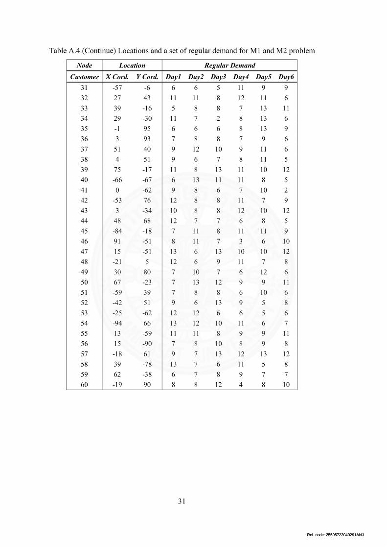
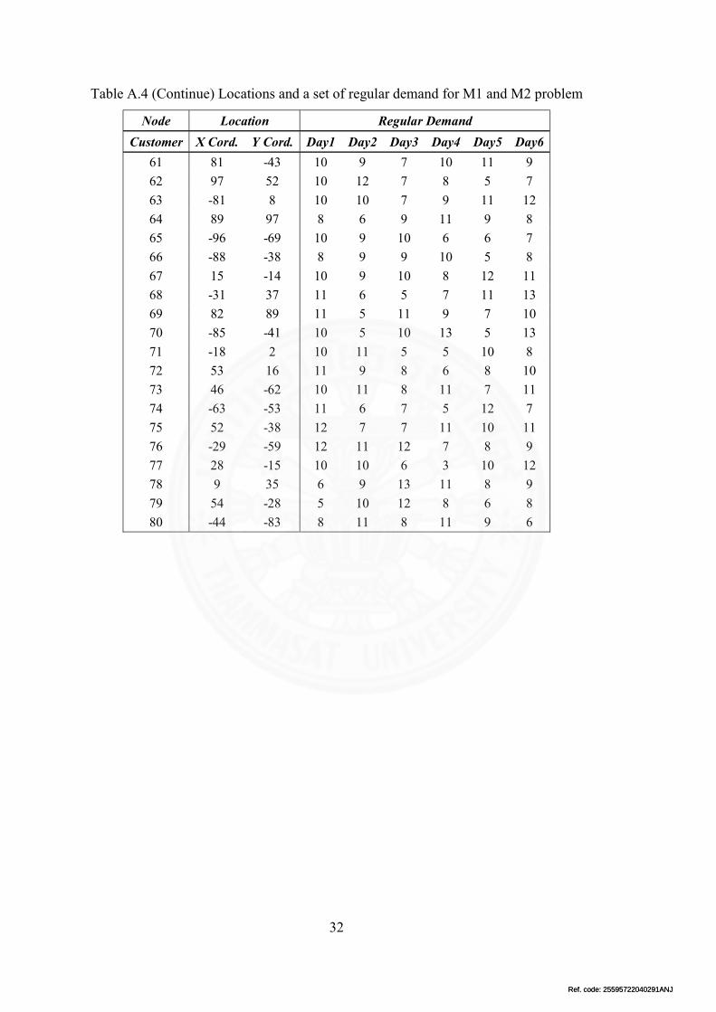
2. The medium problem instances: M1 and M2 problem




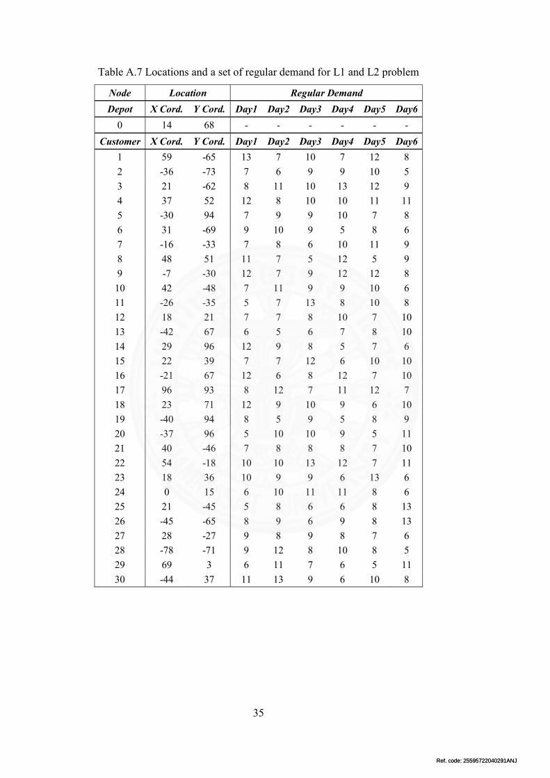
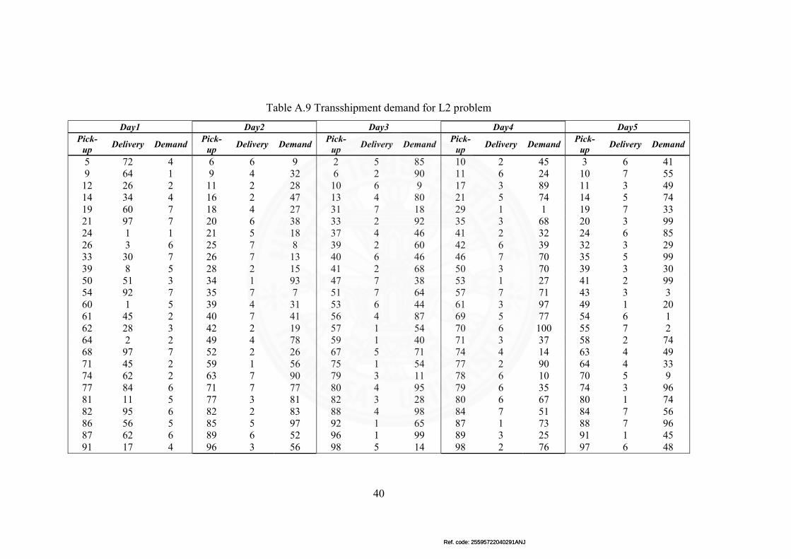
3. The large problem instances: L1 and L2 problem





28

Table A.1 Locations and a set of regular demand for S1 and S2 problem


Depot X Cord. Y Cord. Day1 Day2 Day3 Day4 Day5 Day6

0 14 68 - - - - - -

Customer X Cord. Y Cord. Day1 Day2 Day3 Day4 Day5 Day6

1 -97 52 11 9 10 7 7 11

2 -25 92 12 11 5 8 12 2

3 -89 18 12 5 13 8 9 11

4 66 65 9 7 10 10 7 7

5 -51 7 10 13 12 7 11 13

6 -79 60 6 13 10 5 10 6

7 96 -20 7 5 7 8 7 13

8 43 -35 7 6 6 10 8 8

9 81 -48 10 7 6 10 6 9

10 -14 -80 11 8 7 12 10 10

11 83 -14 9 11 12 12 5 9

12 -46 -89 10 9 9 9 8 8

13 -69 -5 7 13 5 8 8 4

14 1 -22 7 10 9 6 13 10

15 -96 -58 6 11 9 11 10 12

16 31 9 6 6 8 6 5 9

17 -70 41 12 6 7 10 9 8

18 -2 -58 12 9 6 11 8 9

19 -11 -45 8 6 10 6 12 6

20 -94 -35 12 11 7 10 7 6

21 -91 -4 11 7 7 9 7 8

22 9 -84 7 12 10 11 12 8

23 -30 -70 10 8 13 6 12 10

24 10 85 9 7 13 6 5 8

25 99 -32 9 8 12 12 10 11

26 63 8 9 8 11 6 8 9

27 77 -26 8 9 7 10 9 10

28 -27 75 7 7 6 9 7 5

29 -68 62 9 7 10 11 10 11

30 -7 -76 7 13 6 5 11 8


29

Table A.2 Transshipment demand for S1 problem

Day1 Day2 Day3 Day4 Day5

Pick-up Delivery Demand Pick-up Delivery Deman

d Pick-up Delivery

Demand

Pick-up Deliver

y Deman

d Pick-up Delivery

Demand

7 6 7 10 24 4 1 8 4 8 21 6 9 23 2

12 27 4 13 26 5 3 17 3 15 30 2 18 29 4

26 29 2 25 21 7 29 18 1 17 20 5 27 19 1

Table A.3 Transshipment demand for S2 problem

Day1 Day2 Day3 Day4 Day5

Pick-up Delivery Demand Pick-up Delivery Deman

d Pick-up Delivery

Demand

Pick-up Deliver

y Deman

d Pick-up Delivery

Demand

2 22 1 5 29 2 2 22 1 5 29 2 1 20 5

5 1 6 9 16 7 5 1 6 9 16 7 5 14 6

8 30 7 12 6 1 8 30 7 12 6 1 10 15 1

11 2 3 13 11 6 11 2 3 13 11 6 14 30 7

13 18 1 18 30 6 13 18 1 18 30 6 18 17 5

19 17 6 25 18 2 19 17 6 25 18 2 25 7 5

29 18 6 28 29 4 29 18 6 28 29 4 27 29 4


30

Table A.4 Locations and a set of regular demand for M1 and M2 problem



0 14 68 - - - - - -


1 -97 52 11 9 10 7 7 11

2 -25 92 12 11 5 8 12 11

3 -89 18 12 5 13 8 9 11

4 66 65 9 7 10 10 7 7

5 -51 7 10 13 12 7 11 13

6 -79 60 6 13 10 5 10 6

7 96 -20 7 5 7 8 7 13

8 43 -35 7 6 6 10 8 8

9 81 -48 10 7 6 10 6 9

10 -14 -80 11 8 7 12 10 10

11 83 -14 9 11 12 12 5 9

12 -46 -89 10 9 9 9 8 8

13 -69 -5 7 13 5 8 8 9

14 1 -22 7 10 9 6 13 10

15 -96 -58 6 11 9 11 10 12

16 31 9 6 6 8 6 5 9

17 -70 41 12 6 7 10 9 8

18 -2 -58 12 9 6 11 8 9

19 -11 -45 8 6 10 6 12 6

20 -94 -35 12 11 7 10 7 6

21 -91 -4 11 7 7 9 7 8

22 9 -84 7 12 10 11 12 8

23 -30 -70 10 8 13 6 12 10

24 10 85 9 7 13 6 5 8

25 99 -32 9 8 12 12 10 11

26 63 8 9 8 11 6 8 9

27 77 -26 8 9 7 10 9 10

28 -27 75 7 7 6 9 7 10

29 -68 62 9 7 10 11 10 11

30 -7 -76 7 13 6 5 11 8


31

Table A.4 (Continue) Locations and a set of regular demand for M1 and M2 problem



31 -57 -6 6 6 5 11 9 9

32 27 43 11 11 8 12 11 6

33 39 -16 5 8 8 7 13 11

34 29 -30 11 7 2 8 13 6

35 -1 95 6 6 6 8 13 9

36 3 93 7 8 8 7 9 6

37 51 40 9 12 10 9 11 6

38 4 51 9 6 7 8 11 5

39 75 -17 11 8 13 11 10 12

40 -66 -67 6 13 11 11 8 5

41 0 -62 9 8 6 7 10 2

42 -53 76 12 8 8 11 7 9

43 3 -34 10 8 8 12 10 12

44 48 68 12 7 7 6 8 5

45 -84 -18 7 11 8 11 11 9

46 91 -51 8 11 7 3 6 10

47 15 -51 13 6 13 10 10 12

48 -21 5 12 6 9 11 7 8

49 30 80 7 10 7 6 12 6

50 67 -23 7 13 12 9 9 11

51 -59 39 7 8 8 6 10 6

52 -42 51 9 6 13 9 5 8

53 -25 -62 12 12 6 6 5 6

54 -94 66 13 12 10 11 6 7

55 13 -59 11 11 8 9 9 11

56 15 -90 7 8 10 8 9 8

57 -18 61 9 7 13 12 13 12

58 39 -78 13 7 6 11 5 8

59 62 -38 6 7 8 9 7 7

60 -19 90 8 8 12 4 8 10


32

Table A.4 (Continue) Locations and a set of regular demand for M1 and M2 problem



61 81 -43 10 9 7 10 11 9

62 97 52 10 12 7 8 5 7

63 -81 8 10 10 7 9 11 12

64 89 97 8 6 9 11 9 8

65 -96 -69 10 9 10 6 6 7

66 -88 -38 8 9 9 10 5 8

67 15 -14 10 9 10 8 12 11

68 -31 37 11 6 5 7 11 13

69 82 89 11 5 11 9 7 10

70 -85 -41 10 5 10 13 5 13

71 -18 2 10 11 5 5 10 8

72 53 16 11 9 8 6 8 10

73 46 -62 10 11 8 11 7 11

74 -63 -53 11 6 7 5 12 7

75 52 -38 12 7 7 11 10 11

76 -29 -59 12 11 12 7 8 9

77 28 -15 10 10 6 3 10 12

78 9 35 6 9 13 11 8 9

79 54 -28 5 10 12 8 6 8

80 -44 -83 8 11 8 11 9 6


33

Table A.5 Transshipment demand for M1 problem

Day1 Day2 Day3 Day4 Day5 Pick-

up Delivery Demand

Pick-up

Delivery Demand Pick-

up Delivery Demand

Pick-up


up Delivery Demand

10 47 3 5 3 4 5 52 4 5 11 2 12 35 6 16 2 6 15 21 5 13 25 1 7 73 7 14 52 1 33 37 1 21 39 4 18 72 6 18 23 6 15 44 6 42 60 1 22 9 7 26 12 5 30 4 3 27 47 2 43 40 4 27 69 3 38 54 7 34 69 1 41 36 5 46 39 7 42 40 2 48 78 1 57 61 6 49 63 3 59 63 6 77 61 2 66 61 5 62 8 3 52 69 2 73 46 6 80 10 1 73 19 3 76 30 6 57 3 6


34

Table A.6 Transshipment demand for M2 problem


up Delivery Demand

Pick-up


up Delivery Demand

Pick-up


up Delivery Demand

2 45 4 7 8 1 9 40 6 1 52 1 5 70 5 4 63 1 12 20 3 10 78 3 4 29 3 6 4 7 11 7 5 15 23 1 13 57 4 8 19 6 9 24 6 14 29 7 21 73 2 15 21 3 14 19 7 12 40 2 19 16 6 22 5 4 16 36 7 21 49 2 13 60 4 20 11 1 23 53 3 24 47 5 24 76 6 18 63 7 28 53 7 25 2 1 28 9 1 27 5 6 22 58 1 29 59 6 27 66 7 32 34 1 29 37 2 26 61 5 30 27 4 28 9 6 48 35 3 33 12 3 29 71 2 31 42 1 29 34 7 52 80 1 35 11 2 39 2 5 33 42 7 38 54 7 55 74 4 38 33 7 40 55 1 38 24 5 41 13 7 58 37 6 41 73 4 48 50 4 42 1 2 47 9 4 59 20 3 44 51 3 50 14 7 44 22 5 50 45 4 62 41 1 49 43 3 51 1 1 46 8 5 51 80 7 65 58 6 50 35 7 54 9 1 50 64 2 57 77 5 70 65 3 53 55 2 56 73 4 52 29 6 67 9 4 71 53 6 57 23 2 62 78 5 59 41 5 73 65 5 73 56 1 59 80 5 67 13 4 61 56 6 75 45 2 75 65 5 66 21 1 71 19 3 78 54 2 77 70 7 79 27 1 69 18 4 79 39 6


35

Table A.7 Locations and a set of regular demand for L1 and L2 problem



0 14 68 - - - - - -


1 59 -65 13 7 10 7 12 8

2 -36 -73 7 6 9 9 10 5

3 21 -62 8 11 10 13 12 9

4 37 52 12 8 10 10 11 11

5 -30 94 7 9 9 10 7 8

6 31 -69 9 10 9 5 8 6

7 -16 -33 7 8 6 10 11 9

8 48 51 11 7 5 12 5 9

9 -7 -30 12 7 9 12 12 8

10 42 -48 7 11 9 9 10 6

11 -26 -35 5 7 13 8 10 8

12 18 21 7 7 8 10 7 10

13 -42 67 6 5 6 7 8 10

14 29 96 12 9 8 5 7 6

15 22 39 7 7 12 6 10 10

16 -21 67 12 6 8 12 7 10

17 96 93 8 12 7 11 12 7

18 23 71 12 9 10 9 6 10

19 -40 94 8 5 9 5 8 9

20 -37 96 5 10 10 9 5 11

21 40 -46 7 8 8 8 7 10

22 54 -18 10 10 13 12 7 11

23 18 36 10 9 9 6 13 6

24 0 15 6 10 11 11 8 6

25 21 -45 5 8 6 6 8 13

26 -45 -65 8 9 6 9 8 13

27 28 -27 9 8 9 8 7 6

28 -78 -71 9 12 8 10 8 5

29 69 3 6 11 7 6 5 11

30 -44 37 11 13 9 6 10 8


36

Table A.7 (Continue) Locations and a set of regular demand for L1 and L2 problem



31 22 10 8 8 7 12 6 8

32 -40 -55 11 6 8 5 11 12

33 16 5 13 7 8 8 8 13

34 88 -7 6 12 5 11 11 7

35 30 53 11 8 7 10 9 9

36 -55 -31 6 6 6 5 9 13

37 93 67 12 9 7 12 6 6

38 -16 -89 12 13 7 10 10 13

39 84 9 12 6 7 10 8 9

40 -91 -92 13 11 8 11 10 9

41 -69 94 8 8 8 10 6 8

42 74 97 7 5 11 11 7 11

43 14 -16 7 9 12 12 9 12

44 83 67 12 11 12 6 11 10

45 -38 -6 11 11 9 11 10 6

46 -11 56 12 12 8 13 9 13

47 54 85 7 6 12 10 12 11

48 98 -48 5 12 7 7 5 12

49 17 71 9 8 7 7 6 10

50 -39 95 6 7 10 9 7 12

51 32 17 8 11 11 10 8 10

52 -15 71 5 12 5 6 8 8

53 -73 34 5 12 7 5 11 5

54 21 -80 7 12 7 7 9 7

55 -19 86 13 8 8 5 12 9

56 -25 -71 7 9 5 12 9 3

57 -76 -13 11 7 7 8 8 11

58 0 38 12 10 11 7 6 10

59 -67 0 8 10 6 12 8 12

60 -99 33 5 11 12 7 8 9


37




61 38 38 13 6 11 5 13 13

62 -70 -46 6 6 13 11 12 6

63 -83 64 5 8 12 7 11 12

64 -8 89 12 7 6 10 6 10

65 -99 91 7 7 10 7 8 6

66 41 -25 11 8 9 9 12 8

67 -34 -16 8 7 7 6 11 12

68 81 2 13 11 9 12 8 6

69 -56 55 11 10 8 13 8 7

70 -34 8 12 6 12 10 12 11

71 -89 67 12 6 11 8 9 6

72 -1 80 13 5 10 13 6 2

73 -2 34 6 12 10 7 5 12

74 -66 -42 6 5 13 7 12 9

75 -17 19 11 12 7 8 12 12

76 -24 28 7 13 7 5 8 10

77 95 -65 11 11 6 5 7 7

78 -22 -69 10 12 7 7 11 11

79 13 -54 10 6 7 12 10 9

80 44 -46 5 7 13 5 12 6

81 66 65 12 5 10 9 12 9

82 -72 35 6 10 9 11 8 13

83 33 -45 11 11 9 13 12 6

84 35 -38 12 11 8 6 10 6

85 -58 -70 6 10 9 10 12 12

86 17 -26 11 11 8 12 11 8

87 73 -48 9 9 10 11 8 7

88 -21 -40 6 6 7 6 9 6

89 -45 35 10 7 11 8 5 13

90 75 56 13 8 8 9 11 7


38




91 -34 42 9 6 7 7 13 5

92 -92 53 7 8 6 8 9 12

93 -65 87 6 10 10 11 8 4

94 -67 -13 8 6 7 10 6 5

95 -59 -67 12 9 13 8 11 11

96 53 -52 10 13 11 10 8 7

97 -86 -7 11 10 6 13 12 10

98 22 73 6 10 11 9 5 5

99 31 -70 8 7 10 8 9 10

100 45 -49 11 13 11 13 6 5


39

Table A.8 Transshipment demand for L1 problem


up Delivery Demand

Pick-up


up Delivery Demand

Pick-up


up Delivery Demand

22 77 2 1 24 6 1 71 4 4 99 6 4 53 2 39 78 6 16 95 4 3 56 3 8 40 5 22 14 7 40 3 2 36 18 1 17 76 3 40 84 4 28 37 2 54 1 5 44 83 3 38 25 7 42 53 7 51 96 6 62 57 5 47 16 2 40 69 4 47 26 2 70 48 6 85 46 5 56 4 2 48 47 6 48 31 3 80 46 6 88 95 2 87 99 6 55 13 1 55 7 5 82 3 1 93 87 5 90 78 5 67 22 5 73 61 4 92 40 4 96 7 3 93 74 4 97 38 2 77 68 5 95 50 4

100 63 6 98 12 5 98 79 1 79 51 4 99 66 5


40

Table A.9 Transshipment demand for L2 problem


up Delivery Demand

Pick-up


up Delivery Demand

Pick-up


up Delivery Demand

5 72 4 6 6 9 2 5 85 10 2 45 3 6 41 9 64 1 9 4 32 6 2 90 11 6 24 10 7 55

12 26 2 11 2 28 10 6 9 17 3 89 11 3 49 14 34 4 16 2 47 13 4 80 21 5 74 14 5 74 19 60 7 18 4 27 31 7 18 29 1 1 19 7 33 21 97 7 20 6 38 33 2 92 35 3 68 20 3 99 24 1 1 21 5 18 37 4 46 41 2 32 24 6 85 26 3 6 25 7 8 39 2 60 42 6 39 32 3 29 33 30 7 26 7 13 40 6 46 46 7 70 35 5 99 39 8 5 28 2 15 41 2 68 50 3 70 39 3 30 50 51 3 34 1 93 47 7 38 53 1 27 41 2 99 54 92 7 35 7 7 51 7 64 57 7 71 43 3 3 60 1 5 39 4 31 53 6 44 61 3 97 49 1 20 61 45 2 40 7 41 56 4 87 69 5 77 54 6 1 62 28 3 42 2 19 57 1 54 70 6 100 55 7 2 64 2 2 49 4 78 59 1 40 71 3 37 58 2 74 68 97 7 52 2 26 67 5 71 74 4 14 63 4 49 71 45 2 59 1 56 75 1 54 77 2 90 64 4 33 74 62 2 63 7 90 79 3 11 78 6 10 70 5 9 77 84 6 71 7 77 80 4 95 79 6 35 74 3 96 81 11 5 77 3 81 82 3 28 80 6 67 80 1 74 82 95 6 82 2 83 88 4 98 84 7 51 84 7 56 86 56 5 85 5 97 92 1 65 87 1 73 88 7 96 87 62 6 89 6 52 96 1 99 89 3 25 91 1 45 91 17 4 96 3 56 98 5 14 98 2 76 97 6 48

Simulated annealing algorithm for vehicle routing problem ...

Documents

Transcript of Simulated annealing algorithm for vehicle routing problem ...