A Generic Framework for Time-Stepping PDEs:

general linear methods, object-orientated

implementation and application to fluid problems

Peter E.J. Vosa,b, Sehun Chuna, Alessandro Bolisa,

Claes Eskilssonc, Robert M. Kirbyd and Spencer J. Sherwina,∗

aDept. of Aeronautics, Imperial College London, South Kensington Campus, London, SW7 2AZ, UKbFlemish Institute for Technological Research (Vito), Boeretang 200, BE-2400 Mol, Belgium

cDept. of Shipping and Marine Technology, Chalmers Univ. of Tech., SE-412 96 Gothenburg, SwedendSchool of Computing, Univ. of Utah, 50 S. Central Campus Drive, Salt Lake City, UT 84112, USA

October 24, 2010

Abstract

Time-stepping algorithms and their implementations are a criticalcomponent within the solution of time-dependent partial differential equa-tions (PDEs). In this paper we present a generic framework – both interms of algorithms and implementations – that allows an almost seam-lessly switch between various explicit, implicit and implicit-explicit (IMEX)time-stepping methods. We put particular emphasis on how to incorpo-rate time-dependent boundary conditions, an issue that go beyond clas-sical ODE theory but which play an important role in the time-steppingof the PDEs arising in computational fluid dynamics. Our algorithm isbased upon J.C. Butcher’s unifying concept of General Linear Methodsthat we have extended to accommodate the family IMEX schemes thatare often used in engineering practice. In the paper we discuss designconsiderations and presents an object-orientated implementation. Finallywe illustrate the use of the framework by applications to model problemas well as to more complex fluid problems.

1 Introduction

In the development of simulation software into which numerical approximationstrategies for solving time-dependent partial differential equations (PDEs) areutilised, the time-stepping method and its implementation typically receive asubordinate role to the modelling and spatial discretisation choices. There exista myriad of reasons why this partitioning of effort exists and is justified. Inpart, the Method of Lines (MoL), which is commonly employed to help simplifythe discretisation process, focuses one’s attention on distilling the partial differ-ential equations down to a collection of coupled ordinary differential equations

∗Corresponding author. Email: s.sherwin@imperial.ac.uk

1

(ODEs) to which classic time-stepping methods can be applied (see e.g. [25] fordiscussions and examples of the MoL approach). Tremendous effort is investedinto the distillation process of modelling and spatial discretisation, and often isthe final ODE integration stage viewed as a straightforward process requiringlittle concentrated focus.

When ready to start time-stepping the semi-discretized PDE the multi-stage/multi-step divide is encountered – whether to use multi-step methods likeAdams-Bashforth and Adams-Moulton, which typically require more memorybut have an economy of floating-point operations, or to use multi-stage methodslike Runge-Kutta (RK), which typically have larger stability regions and requireless memory. Whichever selection is made might require further reworking ofthe simulation software to accommodate either the memory needs or evaluationneeds of the family of schemes selected. This serves further to discourage fullyexploiting all the advances that have been made in the numerical solution ofODEs and discourages doing verification studies in which the interplay betweenspatial and temporal discretisation errors (beyond just leading order-of-accuracystatements) are quantified.

The goal of this effort was to develop a generic framework, both in termsof algorithms and software implementations, which allows an almost seamlesslyswitch between various explicit and implicit time-stepping methods. The firstchallenge we encountered was the question of how to span the multi-stage/multi-step divide. By basing our algorithms on J.C. Butcher’s unifying General LinearMethods (GLM), as originally introduced by [6], we are able to accommodatea wide range of the time-stepping schemes used in engineering practice, whichnot only encourages the judicious use of the plethora of different methods thatexist, but also facilitates time-discretisation verification studies.

General linear methods, see e.g. [3, 4, 16, 5, 17] and the numerous refer-ences therein, unify the analysis of ODEs with respect to consistency, stabilityand convergence. In addition to GLM covering many of the classical methods, italso includes methods such as the ‘two-step Runge-Kutta methods’ [18], ‘almostRunge-Kutta methods’ [9, 23], ‘diagonally implicit multistage integration meth-ods’ [7, 8] and ‘methods with inherent Runge-Kutta stability’ [30]. Examplesof existing GLM based ODE codes are due to [28, 29, 10, 15, 30]. These codesare highly specialised implementations of a single sub-class of GLMs. We notethat our objective is quite different as we want to use the unifying property ofthe GLMs as foundation for building a generic time-stepping framework.

However, the ODE concept of GLM currently does not encompass the familyof implicit-explicit (IMEX) schemes that are often used to time-integrate PDEs,see e.g. [2, 1, 19]. In order to treat these schemes in a similar way, we have shownthat through a small modification, these schemes as well can be formulated asa general linear method.

Although the MoL approach in principle abstracts away the spatial dis-cretization part of the PDE, there are some specific issues arising during thisprocedure that have a decisive influence on the design of a generic PDE time-stepping framework. In particular, the question how to deal with time-dependentboundary conditions in a generic and computationally efficient manner formsthe second major challenge of this work.

Finally, a remark regarding terminology when dealing with time-steppingschemes that are formally explicit from an ODE point of view. Spatially dis-cretising a PDE using a Galerkin approach generally leads to a ODE system

2

which involves the “inversion” of a global system regardless of the fact that weare using an explicit time-stepping scheme. This situation can be referred to asan indirect explicit method in contrast to the direct explicit method resultingfrom, for example, a standard finite difference discretization.

1.1 Design Considerations

Based upon the aforementioned motivations, we set the following as the objec-tives of our time-stepping framework:

• It should facilitate both explicit/implicit time-stepping and multi-step andmulti-stage schemes, as well as allowing implementation of more elabo-rate partitioning schemes, e.g. IMEX-RK. However, the framework isrestricted to only incorporate implicit schemes in which the stage valuescan be computed in a decoupled fashion. This includes all implicit multi-step schemes and the diagonally implicit multi-stage schemes such as theDiagonally Implicit Runge-Kutta (DIRK) schemes. Fully implicit multi-stage methods, which are rarely adopted in engineering practice, do notfit into the presented framework.

• It should be designed anticipating that the MoL has been used on a PDEto yield a system of coupled ODEs. Therefore the framework should workfor both static and time-dependent, as well as for both weakly and stronglyenforced boundary conditions.

• It should work independent of the spatial discretisation choice (i.e. itshould work with continuous Galerkin and discontinuous Galerkin meth-ods, as well as with finite difference and finite volume methods).

• It should provide an efficient solution for time-stepping PDEs, i.e. thecomputational cost should be comparable to scheme-specific implementa-tions.

1.2 Outline

In this paper, we document the objectives of our framework, provide a briefoverview of general linear methods, and explain how we design and implementa software solution written in an object-oriented language (OOL) that meetsour objectives. The paper is organized as follows. We begin in Section 2 bypresenting Butcher’s idea of general linear methods and we show how IMEXschemes can also be worked into this framework. Section 3 describes the design,algorithms and implementation of the ODE solving framework. In Section 4,we then present how this ODE framework can be modified into a generic PDEtime-stepping framework meeting the objectives. Therefore, we introduce theMoL decomposition of a model problem, and we explain how to deal with time-dependent boundary conditions in a generic and computationally efficient way.In Section 5, we demonstrate the capabilities of the presented framework bypresenting some examples and in Section 6 we summarise and conclude thepresented work.

3

2 General Linear Methods

General linear methods (GLM) have emerged as an effort to connect two maintypes of time integration schemes: linear multi-step method and linear multi-stage method. Linear multi-step methods, such as Adams family of schemes, usethe collection of r input parameters from the previous time-levels to obtain thesolution at the next time-level. On the other hand, linear multi-stage methodssuch as Runge-Kutta methods approximate the solution at the new time-levelby linearly combining the solution at s intermediate stages.

To begin, the standard initial value problem in autonomous form is repre-sented by the ODE,

dy

dt= f(y), y(t0) = y0, (1)

where f : RN → RN . The nth step of the general linear method comprised of r

steps and s stages is then formulated as [3]:

Y i = ∆t

s∑

j=1

aijF j +

r∑

j=1

uijy[n−1]j , 1 ≤ i ≤ s, (2a)

y[n]i = ∆t

s∑

j=1

bijF j +

r∑

j=1

vijy[n−1]j , 1 ≤ i ≤ r, (2b)

where Y i are called the stage values and F i are called the stage derivatives.Both quantities are related by the differential equation:

F i = f(Y i). (2c)

The matrices A = [aij ], U = [uij ], B = [bij ], V = [vij ] are characteristic of aspecific method, and as a result, each scheme can be uniquely defined by thepartitioned (s+ r)× (s+ r) matrix

[

A UB V

]

. (3)

For a more concise notation, it is convenient to define the vectors Y ,F ∈ RsN

and y[n−1]i ,y

[n]i ∈ R

rN as follows:

Y =

Y 1

Y 2

...Y s

, F =

F 1

F 2

...F s

, y[n−1] =

y[n−1]1

y[n−1]2...

y[n−1]r

, and y[n] =

y[n]1

y[n]2...

y[n]r

.

(4)Using these vectors, it is possible to write Eq. (2a) and Eq. (2b) in the form

[

Y

y[n]

]

=

[

A⊗ IN U ⊗ INB ⊗ IN V ⊗ IN

] [

∆tFy[n−1]

]

, (5)

where IN is the identity matrix of dimensionN×N and ⊗ denotes the Kroneckerproduct. Note that it is the first element of the input vector y[n−1] and outputvector y[n] which represents the solution at the corresponding time-level, i.e.

4

y[n]1 = yn = y(t0 + n∆t). The other subvectors y

[n]i (2 ≤ i ≤ r) refer to the

approximation of an auxiliary set of values inherent to the scheme. These values,in general, are comprised of either solutions or derivatives at earlier time-levelsor a combination hereof. Many well-known, as well as lesser known, schemescan be cast as a GLM, see Appendices A.1-A.3.

2.1 Implicit-explicit general linear methods

In this section, we extend the idea of GLM to accommodate in addition implicit-explicit (IMEX) schemes. IMEX schemes [2, 1] were introduced to time-integrateODEs of the form

dy

dt= f(y) + g(y), y(t0) = y0, (6)

where f : RN → RN typically is a non-linear function and g : RN → R

N is astiff term (or where f and g have disparate time-scales). The idea behind IMEXmethods is to combine two different type of schemes: one would like to use animplicit scheme for the stiff term in order to avoid an excessively small time-step. At the same time, explicit integration of the non-linear term is preferredto avoid its expensive inversion.

Following the same underlying idea as discussed in the previous sections,IMEX linear multi-step schemes [2] and IMEX Runge-Kutta schemes [1] can beunified into an IMEX general linear method formulation, i.e.

Y i = ∆t

s∑

j=1

aIMij Gj +∆t

s∑

j=1

aEXij F j +

r∑

j=1

uijy[n−1]j , 1 ≤ i ≤ s, (7a)

y[n]i = ∆t

s∑

j=1

bIMij Gj +∆t

s∑

j=1

bEXij F j +

r∑

j=1

vijy[n−1]j , 1 ≤ i ≤ r, (7b)

where the stage derivatives F i and Gi are defined as

F i = f(Y i), Gi = g(Y i), (7c)

and where the superscripts IM and EX are used to denote implicit and explicitrespectively. Adopting a matrix formulation similar to that shown in Eq. (5),this can be written in the form

[

Y

y[n]

]

=

[

AIM ⊗ IN AEX ⊗ IN U ⊗ IN

BIM ⊗ IN BEX ⊗ IN V ⊗ IN

]

∆tG

∆tF

y[n−1]

. (8)

To further illustrate the formulation of IMEX schemes as a GLM, a few examplesare given in Appendix A.4.

3 A generic ODE solving framework

Just as Butcher’s general linear methods provide a general framework to studythe basic properties such as consistency, stability and convergence of differentfamilies of numerical methods for ODEs, it can also serve as a starting pointfor a unified numerical implementation. For maximum generality we base our

5

implementation on the IMEX-GLM formulation described in Section 2.1: forpurely explicit methods we simply define AIM, BIM as well as g(y) equal tozero. For purely implicit schemes we analogously set AEX, BEX and f(y) to bezero.

3.1 Evaluation of general linear methods

Inspecting Eq. (7) it can be appreciated that a single step from level n − 1 ton for an IMEX-GLM formulation can be evaluated through the following algo-rithm:

input : the vector y[n−1]

output: the vector y[n]

// Calculate stage values Y i and the stage derivatives F i

and Gi

for i = 1 to s do

// calculate the temporary variable xi

(A1.1) xi = ∆t∑i−1

j=1 aIMij Gj +∆t

∑i−1j=1 a

EXij F j +

∑rj=1 uijy

[n−1]j

// calculate the stage value Y i

(A1.2) solve(

Y i − aIMii ∆tg(Y i))

= xi

// calculate the explicit stage derivative F i

(A1.3) F i = f(Y i)

// calculate the implicit stage derivative Gi

(A1.4) Gi = g(Y i) =1

aIM

ii∆t

(Y i − xi)

end

// Calculate the output vector y[n]

for i = 1 to r do

// calculate y[n]i

(A1.5) y[n]i = ∆t

∑sj=1 b

IMij Gj +∆t

∑sj=1 b

EXij F j +

∑rj=1 vijy

[n−1]j

end

Algorithm 1: A GLM-based ODE solving algorithm.

Here we first observe that the algorithm, by virtue of the GLM framework,is independent of the actual numerical scheme used – only the values of thecoefficients a and b change for different methods. Further, if we are using apurely explicit scheme then aIMii = 0 and the stage value is equal to the thetemporary value computed in step (A1.1), i.e. step (A1.2) is greatly simplifiedto Y i = xi. It is also worth noting that the stage derivative Gi = g(Y i)in (A1.4) need not be explicitly evaluated, but is given by already computedvalues, as seen by reordering Eq. (A1.2). Indeed, steps (A1.2) and (A1.3) arethe only instances in the algorithm where specific information from the ODE isrequired, all other steps in the algorithm simply involve linear combinations ofprecomputed information. These two steps are to be considered external parts

6

representing the ODE rather than being a part of the numerical GLM algorithm.We thus need to define the following external functions:

• If AIM 6= 0 we must supply a routine for solving a system of form (A1.2),

(Y − λg(Y )) = x, (9)

for Y ∈ RN , given as input the vector x ∈ R

N and the scalar λ ∈ R.g : RN → R

N denotes the function prescribing the terms of the ODE thatare to be implicitly evaluated. In general, the solution or fixed point ofthis system can be found through root finding algorithms. In the case g isa linear operator, one may opt for a direct solution method to solve thissystem through the inverse operator (I − λg)−1, where I : RN → R

N isthe identity function.

• If AEX 6= 0 we must also supply a routine for evaluating (A.1.3), i.e. afunction f : RN → R

N that maps the stage values to the stage derivativesfor the terms of the ODE that are explicitly evaluated

F = f(Y ). (10)

The external functions are specific for the ODE under consideration and have tobe specified to the framework. The decoupling of the external components fromthe GLM algorithm naturally leads to a level of abstraction allowing a genericobject-oriented implementation, in a programming language such as C++, tobe discussed in the next section.

3.2 Encapsulation of key concepts

As outlined in the introduction, it is our goal to implement an ODE solvingtoolbox where switching between numerical schemes is as simple as changing aninput parameter. To accomplish this, we have encapsulated the key conceptsobserved in the previous section into a set of C++ type classes, depicted in Fig.1. It is not our intention to necessarily advocate using only C++ but ratherto highlight how any OOL could be used to encapsulate the concepts. Weacknowledge that many OOL exist which could be used for this implementationstage.

3.2.1 The class TimeIntegrationOperators

This class provides a general interface to the external components (see Section3.1) needed for time marching. As a result, this class can be seen as the ab-straction of the ODE. As data members, it contains two objects which can bethought of as function pointers : m_explicitEvaluate should point to the im-plementation of (10) and m_implicitSolve should point to the implementationof solving system (9). Note that the actual routines pointed to by the functionpointers are not part of the framework and must be provided as they are spe-cific for each ODE under consideration. The function pointers can be linkedto these implementations by means of the methods DefineExplicitEvaluateand DefineImplicitSolve. The encapsulation of these functions into another

7

m inputTimeLevels

data members

methods

class

data members

methods

GetSolution

classTimeIntegrationSolution

data members

m A

m B

classTimeIntegrationScheme

m implicitSolve

m explicitEvaluate

DefineExplicitEvaluate

DefineImplicitSolve

DoExplicitEvaluate

DoImplicitSolve

TimeIntegrationOperators

m solutionvector

methods

m U

m V

InitializeScheme

TimeIntegrate

Figure 1: Overview of the classes in the implementation of the generic ODEsolving framework.

class is needed to ensure that both these functions can be accessed from withinthe time-stepping algorithms in a unified fashion, independent of which ODEis being solved. Therefore, the class TimeIntegrationOperators also containsthe methods DoExplicitEvaluate and DoImplicitSolve for internal use.

3.2.2 The class TimeIntegrationSolution

This class is the abstraction of the vector y[n] as defined in Eq. (4). One

can think of it as an array of arrays. The first entry y[n]1 = yn represents

the approximate solution at time-level n, and can be obtained by means of themethod GetSolution.

3.2.3 The class TimeIntegrationScheme

This class can be considered as the main class as it is the abstraction of a generallinear method. As each scheme is uniquely defined by the partitioned coefficientmatrix (3), the sub-matrices A, B, U and V are core data members of thisclass, implemented respectively as m_A, m_B, m_U and m_V. In addition, this classcontains the data member m_inputTimeLevels which reflect the structure of theinput/output vector y[n] associated to the scheme. Based upon the fact that allinput vectors can be ordered such that the stage values are listed first before theexplicit stage derivatives and the implicit stage derivatives, m_inputTimeLevelscan be seen as an array existing of three parts that indicate the time-levelat which the values/derivatives are evaluated. As an example, consider thesecond-order Crank-Nicholson/Adams-Bashforth scheme with input vector y[n]

as defined in Eq. (73). The data member m_inputTimeLevels is then definedas

m_inputTimeLevels =

0001

. (11)

Furthermore, this class is equipped with the two methods needed for the actualtime-marching. The function InitializeScheme converts the initial value y0 in

8

an object of the class TimeIntegrationSolution. This object is then going tobe advanced in time using the method TimeIntegrate. It is the TimeIntegratemethod which actually implements the GLM algorithm in Section 3.1 and henceintegrates the ODE for a single time-step. Note that internally, this methodcalls the functions DoExplicitEvaluate and DoImplicitSolve of the classTimeIntegrationOperators in order to evaluate Eq. (10) and solve Eq. (9)respectively.

3.3 Use of the framework

As mentioned earlier the functionality described by Eqs. (9) and (10) are ODEspecific and must be implemented and provided to the framework according tothe prototype defined in Code 1.

Code 1 Prototype of functions required to be provided by the user

double* ExplicitEvaluate(double* x)

... // ODE specific implementation

double* ImplicitSolve(double* x, double lambda)

... // ODE specific implementation

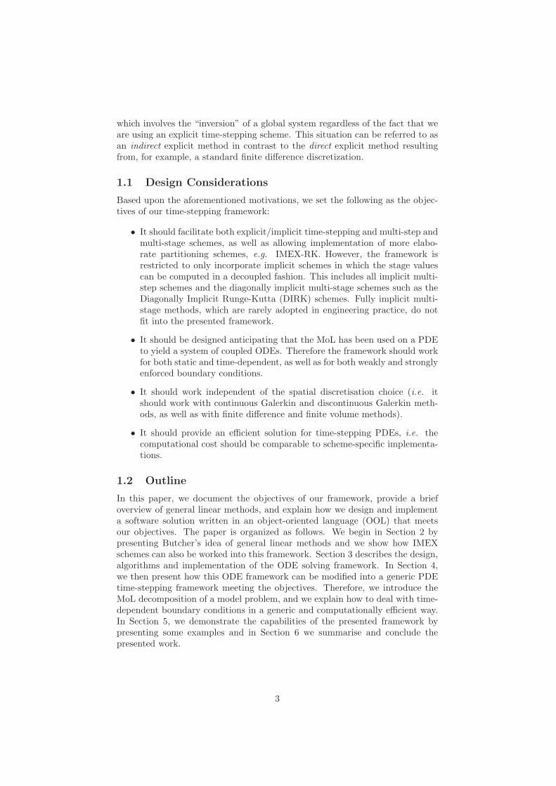
These functions, together with the classes of the toolbox, can then be usedto numerically solve the ODE. A typical example of this is shown in the exampleCode 2. In this particular example, the constructor call

scheme = TimeIntegrationScheme(FORWARD_EULER)

loads the object with the coefficient matrices of the forward Euler scheme. How-ever, none of the external ODE specific implementation changes when selectinga more advanced time-stepping method. Other schemes can simply be loaded bychanging the input argument (e.g. from FORWARD_EULER to CLASSICAL_RK_4).This example illustrates how the presented framework can be used to numer-ically solve an ODE in a unified fashion, independent of the chosen scheme.

3.3.1 Initiating multi-step schemes

For multi-step schemes, a slight modification is required to properly start-up thesystem. In the framework we use the classic start-up procedure of employingthe first k − 1 step of a k-step multi-step scheme using a kth order multi-stage scheme, as illustrated for the third-order Adams-Bashforth scheme in theexample Code 3. For non-stiff problem we use an explicit RK scheme while forstiff problems the start-up could be performed by means of a DIRK scheme.

Underneath, this starting-up procedure is founded upon the data memberm_inputTimeLevels. When making the call

9

Code 2 Example demonstrating how the framework can be used to solve anODE

TimeIntegrationOperators ode;

TimeIntegrationSolution y_n;

TimeIntegrationScheme scheme;

ode.DefineExplicitEvaluate(&ExplicitEvaluate);

ode.DefineImplicitSolve(&ImplicitSolve);

scheme = TimeIntegrationScheme(FORWARD_EULER);

y_n = scheme->InitializeScheme(dt,y_0,ode);

for(n = 0; n < nsteps; ++n)

scheme->TimeIntegrate(dt,y_n,ode);

Code 3 Example demonstrating the initiation of multi-step schemes.

scheme = TimeIntegrationScheme(ADAMS_BASHFORTH_ORDER3);

startup_scheme = TimeIntegrationScheme(RK_ORDER3);

y_n = scheme->InitializeScheme(dt,y_0,ode);

startup_scheme->TimeIntegrate(dt,y_n,ode); // step n = 0

startup_scheme->TimeIntegrate(dt,y_n,ode); // step n = 1

for(n = 2; n < nsteps; ++n)

scheme->TimeIntegrate(dt,y_n,ode);

startup_scheme1->TimeIntegrate(dt,y_n,ode)

the TimeIntegrate routine recognises that the input vector y_n is initialisedaccording to another scheme. It is therefore going first to construct an inputvector according to the start-up scheme, and it will map the information fromthe vector y_n to the newly constructed input vector, thereby making use of thedata member m_inputTimeLevels. If the start-up scheme requires informationin its input vector that is not available in the provided input vector y_n it willsimply assume zero for these stage values or derivatives. Once the solution isadvanced in time for a single time-step using the start-up scheme, the outputvector is mapped back to the vector y_n, again making use of the informationin m_inputTimeLevels.

The start-up procedure effectively integrates the ODE k− 1 steps. If this isnot desirable then the derivatives in y[0] must be estimated by a more elaboratestarting procedure, see e.g. [28, 30, 17].

10

4 Time-dependent partial differential equations

Ordinary differential equations are generally used to model initial value prob-lems. However, many physical processes can be regarded as initial boundaryvalue problems which are described by partial differential equations. A firststep in solving time-dependent PDEs consists of reducing the PDE to a systemof ODEs through the MoL approach. For this procedure, which involves thediscretisation of the spatial dimensions, we will primarily adopt the spectral/hpelement method [21] in this work. We will show that the application of the MoLintroduces some typical issues which prevent the straightforward application ofthe ODE framework discussed before. We distinguish the following issues:

• strongly enforced essential boundary conditions, and

• computational efficiency.

To facilitate the discussion we will use the scalar advection-diffusion equationas an illustrative example throughout this section. It is given by

∂u

∂t+∇ · F (u) = ∇2u, in Ω× [0,∞), (12a)

u(x, t) = gD(x, t), on ∂ΩD × [0,∞), (12b)

∂u

∂n(x, t) = gN (x, t) · n, on ∂ΩN × [0,∞), (12c)

u(x, 0) = u0(x), in Ω, (12d)

where Ω is a bounded domain of Rd with boundary ∂Ω = ∂ΩD

⋃

∂ΩN and n de-notes the outward normal to the boundary ∂Ω. Furthermore, we will abbreviatethe advection term as f(u) = −∇ · F (u) in the following sections.

4.1 The Method of Lines

We start with a (possibly high-order) finite element approach to reduce theadvection-diffusion equation (12) to a system of ODEs using the MoL. Followingthe standard Galerkin formulation we multiply Eq. (12a) by a smooth testfunction v(x), which by definition is zero on all Dirichlet boundaries. Integratingover the entire spatial domain leads to the following variational formulation:Find u ∈ U such that

∫

Ω

v∂u

∂tdx−

∫

Ω

vf(u)dx =

∫

Ω

v∇2udx, ∀v ∈ V, (13)

where U and V are suitably chosen trial and test spaces respectively. We obtainthe weak form of the diffusion operator by applying the divergence theorem tothe right-hand-side term yielding: Find u ∈ U such that

∫

Ω

v∂u

∂tdx−

∫

Ω

vf(u)dx = −∫

Ω

∇v · ∇udx+

∫

∂Ω

v∇u · ndx, ∀v ∈ V. (14)

As v(∂ΩD) is equal to zero, only Neumann conditions will give contributions tothe boundary integral, and we enforce the conditions weakly through substitut-ing ∇u = gN in the boundary integral. In order to impose Dirichlet boundary

11

conditions one can choose to adopt a lifting strategy where the solution is de-composed into a known function, uD and an unknown homogeneous functionuH , i.e.

u(x, t) = uH(x, t) + uD(x, t). (15)

Here uD satisfies the Dirichlet boundary conditions, uD(∂ΩD) = gD, and thehomogeneous function is equal to zero on the Dirichlet boundary, uH(∂ΩD) = 0.The weak form (14) can then be formulated as: Find uD ∈ U0 such that,∫

Ω

v∂(uH + uD)

∂tdx−

∫

Ω

vf(uH + uD)dx =−∫

Ω

∇v · (∇uH +∇uD)dx

+

∫

∂ΩN

vgN · ndx, ∀v ∈ V.

(16)

Following a finite element discretisation procedure, the solution is expandedin terms of a globally C0-continuous expansion basis Φi that spans the finitedimensional solution space Uδ. We also decompose this expansion basis into thehomogeneous basis functions ΦH

i and the basis functions ΦDi having support on

the Dirichlet boundary such that

uδ(x, t) =∑

i∈NH

ΦHi (x)uH

i (t) +∑

i∈ND

ΦDi (x)uD

i (t). (17)

Finally, employing the same expansion basis ΦHi to span the test space V, Eq.

(16) leads to the semi-discrete system of ODEs

[

MHD MHH] d

dt

[

uD

uH

]

= −[

LHD LHH]

[

uD

uH

]

+ ΓH + fH

(18)

where

MHH [i][j] =

∫

Ω

ΦHi ΦH

j dx i ∈ NH , j ∈ NH ,

MHD[i][j] =

∫

Ω

ΦHi ΦD

j dx i ∈ NH , j ∈ ND,

LHH [i][j] =

∫

Ω

∇ΦHi · ∇ΦH

j dx i ∈ NH , j ∈ NH ,

LHD[i][j] =

∫

Ω

∇ΦHi · ∇ΦD

j dx i ∈ NH , j ∈ ND,

fH[i] =

∫

Ω

ΦHi f(u)dx i ∈ NH

ΓH [i] =

∫

∂ΩN

ΦHi gN · ndx i ∈ NH .

This can be rewritten in terms of the unknown variable uH as

duH

dt=(

MHH)−1

−[

LHD LHH]

[

uD

uH

]

+ ΓH + fH −MHD duD

dt

,

(19)which, in the absence of Dirichlet boundary conditions, simplifies to

du

dt= −M−1 (Lu− Γ) +M−1f (20)

12

4.2 Use of the ODE framework for time integrating PDEs

At first sight, it may seem feasible to apply ODE framework of Section 3 totime-integrate Eq. (19) (or Eq. (20)). However, this straightforward approachappears to lead to two problems.

4.2.1 Computational efficiency

Considering Eq. (20) in the context of the IMEX algorithm of the ODE frame-work (Algorithm 1), it can be appreciated that for the explicit advection term,step (A.1.4) requires the calculation of the term

M−1f , (21)

while for the implicit diffusion term, step (A.1.2) would require solving a systemof the form

(

I +∆tM−1L)

u = x. (22)

It appears that next to the implicit term, the explicit term now also requiresa global matrix inverse due to M−1. This means that the generic ODE time-stepping algorithm would require two global matrix inverses at every timestep/timestage.For comparison, let us consider the (single-stage) first-order Backward Eu-ler/Forward Euler IMEX scheme given by Eq. (70). A scheme-specific imple-mentation of this method (that is, not making use of the proposed framework)can integrate Eq. (20) for a single time-step as

un = (M +∆tL)−1(

Mun−1 +∆tfn−1 +∆tΓn

)

. (23)

Clearly, this only involves a single global matrix inversion, i.e. (M +∆tL)−1

.Such global matrix inversions can be assumed to be the critical cost of the time-integration process as they typically –especially for three-dimensional simulations–require an iterative solution method which induce a far bigger cost than the other“forward” operations. Because of this substantial performance penalty, usingthe ODE framework to time-integrate PDEs can be argued to be impractical.

4.2.2 Time-dependent Dirichlet boundary conditions

The second complication with applying the framework to time integrate Eq.

(19) or (20) arises from the term duD

dtin Eq. (19) which is due to a strong

imposition of the Dirichlet boundary conditions. Although the value uD(t) of

the Dirichlet boundary conditions would typically be given for arbitrary t, a

prescription of its time rate-of-change duD

dtis not usually available. This again

prevents a straightforward application of the presented ODE framework.

4.3 A generic PDE time-stepping framework

In order to alleviate both the issues of efficiency and time-dependent boundaryconditions, we propose a modified framework designed to time-integrate PDEsin a generic and efficient manner. The new framework is largely founded on thefact that a finite or spectral/hp element approximation uδ(x, t) can be describednot only by a set of global degrees of freedom u (in coefficient space), but also

13

by a set of nodal values u (in physical space). These nodal values representthe spectral/hp solution at a set of quadrature points xi (or collocation points),such that they can be related to the global coefficients as

u[i] = uδ(x, t) =∑

j∈N

Φj(xi)ui(t), (24)

which, in matrix notation, can be written as u = Bu, where B[i][j] = Φj(xi).In case of a lifted Dirichlet solution, this becomes

u =[

BD BH]

[

uD

uH

]

, (25)

with BD[i][j] = ΦDj (xi) and BH [i][j] = ΦH

j (xi).As commonly is the case in finite or spectral/hp methods, we will also use

this nodal interpretation for the explicit treatment of the (non-linear) advection

term. The term f in Eq. (20) will then be computed as

f = B⊤Wf , (26)

where f represents the original advection term evaluated at the quadraturepoints, i.e. f [i] = f(u(xi)), and W is a diagonal matrix containing the quadra-ture weights needed for an appropriate numerical evaluation of the integral.Such a collocation approach is also known as the pseudo-spectral method [14].

4.3.1 The Helmholtz problem and the projection problem

Before we derive the new framework, we will first introduce the following twoconcepts which will facilitate the derivation.

The Galerkin projection Consider the discrete solution space Uδ(Ω, t) ofC0-continuous piecewise polynomial functions that satisfy the (possibly time-dependent) Dirichlet boundary conditions. In a finite or spectral/hp methodswe typically define the projection of an arbitrary function f(x), denoted as

u = P(f, t), (27)

as the L2 projection of f onto Uδ(Ω).This projection is equivalent to solving the following minimisation problem

using a traditional Galerkin finite element approach: Find u ∈ Uδ(Ω) such that||u − f ||L2 is minimal. In a nodal/collocated context, this projection can becomputed as:

• in case of strongly enforced Dirichlet boundary conditions

u = P(f , t) =[

BD BH]

uD(t)

(

MHH)−1

(

BH)⊤

Wf −MHDuD(t)

,

(28)

• which in the absence of strongly enforced Dirichlet boundary conditions,simplifies to

u = P(f , t) = BM−1B⊤Wf . (29)

14

The Galerkin Helmholtz problem Given an arbitrary function f , we definethe Helmholtz problem as finding the Galerkin finite element solution to the(steady) elliptic Helmholtz equation

u− λ∇2u = f, in Ω, (30a)

u(x) = gD(x), on ∂ΩD, (30b)

∂u

∂n(x) = gN (x) · n, on ∂ΩN . (30c)

We will also denote this problem as

u = H(f, λ, t). (31)

Once again evaluating the solution at nodal/collocation points, this problemcan be discretely evaluated as

• in case of strongly enforced Dirichlet boundary conditions

u = H(f , λ, t) =[

BD BH]

uD(t)

(

HHH)−1

(

BH)⊤

Wf + λΓH(t)−HHDuD(t)

,

(32)

• which in the absence of strongly enforced Dirichlet boundary conditions,simplifies to

u = H(f , λ, t) = BH−1(

B⊤Wf + λΓ(t))

. (33)

In the expressions above, the matrix H represents the Helmholtz matrix definedas

H[i][j] =

∫

Ω

ΦiΦj + λ∇Φi · ∇Φjdx i, j ∈ N . (34)

Properties We will use the following properties of the operators P and H inthe subsequent sections:

• In case λ = 0, the operator H reduces to the projection operator P , i.e.

H(f , 0, t) = P(f , t). (35)

• The operators can be shown to have the following properties:

P(P(f , tm), tn) = P(f , tn), (36)

H(P(f , tm), tn) = H(f , tn) (37)

,P(g +P(f , tm), tn) = P(g + f , tn), and (38)

H(g +P(f , tm), tn) = H(g + f , tn). (39)

15

4.3.2 Derivation of the framework

According to Eq. (7a), the calculation of the ith stage (for convenience ofnotation denoted as u

Hi ) of an arbitrary GLM applied to Eq. (19) can be

represented as

uHi =∆t

i∑

j=1

aIMij

(

MHH)−1

gHj − MHD duD

dt

∣

∣

∣

∣

∣

j

+∆t

i−1∑

j=1

aEXij

[

(

MHH)−1

fH

j

]

+

r∑

j=1

uijuH[n−1]j , (40)

where for simplicity we have used the notation

gHj = −

[

LHD LHH]

[

uDj

uHj

]

+ ΓHj . (41)

For generality we will assume a GLM with an input/output vector of the form

uH[n] =

uHn

uHn−1

∆tGn

∆tGn−1

∆tF n

∆tF n−1

, (42)

which applied to the advection-diffusion example under consideration, leads to

uH[n] =

uHn

uHn−1

∆t(

MHH)−1

(

gHn − MHD duD

dt

∣

∣

∣

∣

∣

n

)

∆t(

MHH)−1

(

gHn−1 − MHD duD

dt

∣

∣

∣

∣

∣

n−1

)

∆t(

MHH)−1

fH

n

∆t(

MHH)−1

fH

n−1

. (43)

In order to deal with the time-derivative of the Dirichlet boundary condition,we first would like to note that we have chosen to treat the term involvingduD

dtimplicitly in Eq. (40). However, this is an arbitrary choice and we could

equally well have chosen to treat this term explicitly, leading to exactly the sameframework. If we then acknowledge that the variable u

D can be understood tosatisfy the ODE

(

uD)′

=duD

dt, (44)

we can apply the same GLM to this ODE as the one we have used for theoriginal ODE in terms of uH , i.e. Eq. (40), to arrive at

uDi = ∆t

i∑

j=1

aIMijduD

dt

∣

∣

∣

∣

∣

j

+

r∑

j=1

uijuD[n−1]j . (45)

16

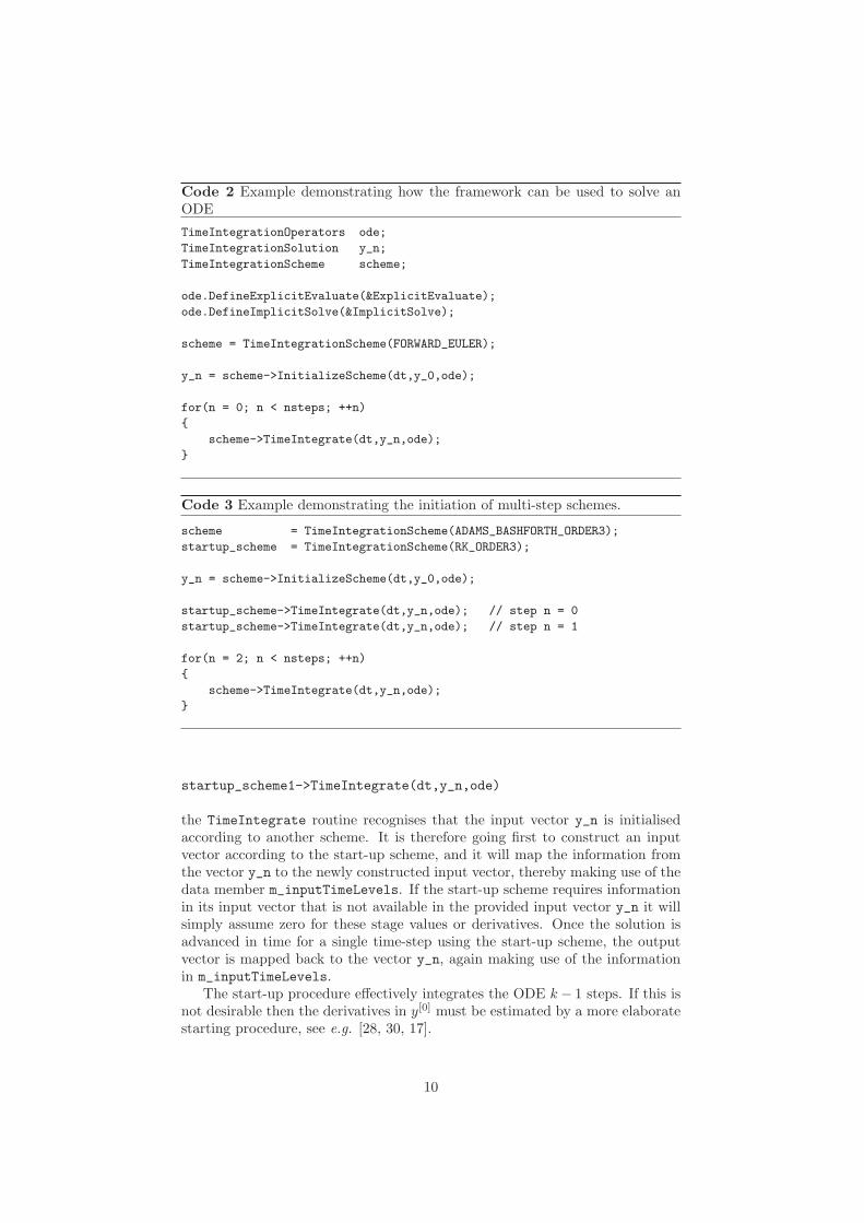
There are no explicit stage derivatives F j appearing in the equation above (ormore precisely, F j = 0) due to the fact that we also choose to treat the right-

hand-side termduD

dtin Eq. (44) implicitly. As a result, the input/output vector

of the GLM under consideration, see Eq. (42), applied to Eq. (44) takes theform

uD[n] =

uDn

uDn−1

∆tduD

dt

∣

∣

∣

∣

∣

n

∆tduD

dt

∣

∣

∣

∣

∣

n−1

00

. (46)

To eliminate the Dirichlet derivative in Eq. (40), we substitute Eq. (45) intoEq. (40), yielding

uHi =∆t

i∑

j=1

aIMij

[

(

MHH)−1

gHj

]

+∆t

i−1∑

j=1

aEXij

[

(

MHH)−1

fH

j

]

+(

MHH)−1

MHD

r∑

j=1

uijuD[n−1]j − u

Di

+r∑

j=1

uijuH[n−1]j , (47)

which after rearranging and multiplication with MHH leads to

MHH uHi +MHDu

Di =∆t

i∑

j=1

aIMij gHj +∆t

i−1∑

j=1

aEXij f

H

j

+r∑

j=1

uij

[

MHH uH[n−1]j +MHDu

D[n−1]j

]

, (48)

or

HHH uHi +HHDu

Di =∆t

i−1∑

j=1

aIMij gHj +∆t

i−1∑

j=1

aEXij f

H

j

+

r∑

j=1

uij

[

MHH uH[n−1]j +MHDu

D[n−1]j

]

+ aIMii ∆tΓHi ,

(49)

where H is the Helmholtz matrix, see Eq. (34), with λ = aIMii ∆t. This

elimination ofduD

dtappears to give rise to a modified input/output vector

MHH uH[n−1]j + MHDu

D[n−1]j , which after combining Eq. (43) and Eq. (46)

17

can be appreciated to be equal to

MHH uH[n] +MHDu

D[n] =

MHH uHn +MHDu

Dn

MHH uHn−1 +MHDu

Dn−1

∆tgHn

∆tgHn−1

∆tfH

n

∆tfH

n−1

. (50)

Following a collocation approach to calculate the advection term, see Eq. (26),and adopting a nodal interpretation for the solution values at the time-levels nand n− 1 according to Eq. (25), this input/output vector can be considered asthe inner product of an input/output vector u[n] in physical space, i.e.

MHH uH[n]+MHDu

D[n] =(

BH)⊤

Wu[n] =(

BH)⊤

W

un

un−1

∆tgn

∆tgn−1

∆tfn

∆tfn−1

, (51)

where we have made use of the relationship MHD =(

BH)⊤

WBD. In ad-

dition, we have also adopted a nodal interpretation gn of the implicit stagevalue gH

n which will be further discussed in the next section. Making use of thisformulation in physical space, Eq. (49) can be written as

HHH uHi +HHDu

Di =

(

BH)⊤

W

∆t

i−1∑

j=1

aIMij gj +∆t

i−1∑

j=1

aEXij f j +

r∑

j=1

uijuj

+aIMii ∆tΓHi . (52)

Finally also adopting a nodal interpretation ui for the solution at stage i, thecalculation of the ith stage value can be recognised as

ui = H

∆ti−1∑

j=1

aIMij gj +∆ti−1∑

j=1

aEXij f j +

r∑

j=1

uijuj , aIMii ∆t, tn

. (53)

This formulation allows for a well defined procedure to advance the solution intime as the calculation of the stage values only involves solving the associatedHelmholtz problem. Note that for a pure explicit method, the Helmholtz prob-lem reduces to the L2 projection. This solution procedure is very attractive inparticularly for the following three reasons:

• uniform treatment of Dirichlet boundary conditions (i.e. the Dirichletboundary conditions only come into play when enforcing them while solv-ing the global matrix system),

• only one global matrix inverse is required per stage, and

• it is sufficiently generic to be extended to the entire range of GLMs (seenext section).

18

Note that the derivation of this framework was founded on the following twosteps:

• adopting a consistent-order discretisation of the Dirichlet derivative con-sistent to the discretisation of the original ODE, and

• formulating the GLM algorithm in physical space.

4.3.3 Algorithm

A PDE time-stepping algorithm that time-integrates the advection-diffusionequation (12) from time-level n− 1 to n can then be formulated as:

input : the vector u[n−1]

output: the vector u[n]

// Calculate stage values U i and the stage derivatives F i

and Gi

for i = 1 to s do

// calculate the temporary variable xi

(A2.1) xi = ∆t∑i−1

j=1 aIMij Gj +∆t

∑i−1j=1 a

EXij F j +

∑rj=1 uiju

[n−1]j

// calculate the stage value U i

(A2.2) U i = H(

xi, aIMii ∆t, ti

)

// calculate the explicit stage derivative F i

(A2.3) F i = f(U i)

// calculate the implicit stage derivative Gi

(A2.4) Gi =1

aIM

ii∆t

(U i − xi)

end

// Calculate the output vector u[n]

if last stage equals new solution then(A2.5) un = U s

else

(A2.6) u[n]1 = u

[n]1 =

P

(

∆t∑s

j=1 bIM1j Gj +∆t

∑sj=1 b

EX1j F j +

∑rj=1 v1ju

[n−1]j , tn

)

end

for i = 2 to r do

(A2.7) u[n]i = ∆t

∑sj=1 b

IMij Gj +∆t

∑sj=1 b

EXij F j +

∑rj=1 viju

[n−1]j

end

Algorithm 2: A GLM based PDE time-stepping algorithm

The only subtlety that arises in comparison with the backward/forward Eulerexample of the previous section is due to the term Gi. To formally fit into theframework, a proper definition of Gi, denoted as Gi, should be

Gi = BH(

MHH)−1

gHi , (54)

19

with gHi as defined in Eq. (41). By recombining the terms in the Helmholtz

problem associated to step (A2.2) it can be demonstrated that this term can beevaluated as

Gi = P

(

U i − xi

aIMii ∆t, ti

)

, (55)

which corresponds to the L2 projection of our initial definition of Gi, i.e. Gi =P (Gi, t) However, do due the properties (38-39) it can be appreciated thatusing Gi in steps (A2.1), (A2.6) and (A2.7) is equivalent to the use of Gi,thereby keeping the number of global system inverses per stage to one.

Comparing this PDE time-stepping algorithm with the original ODE algo-rithm (Algorithm 1), one can identify the following differences:

• While step (A1.2) of the original algorithm essentially is a pure algebraicproblem (that is, for schemes with an implicit component), step (A2.2)also as an broader analytical interpretation in the sense that it is thesolution of the elliptic Helmholtz partial differential equation.

• It has been indicated before that for purely explicit time-stepping methods(i.e. aIMII = 0), the evaluation of step (A1.1) actually vanishes as it isreduced to Y i = xi. However, in the new algorithm, step (A2.2) now alsorequires a global system inverse, as the Helmholtz problem is reduced tothe projection problem for explicit schemes.

• In addition, step (A2.6) of the new algorithm also requires a L2 projection.This is necessary to ensure that the solution is in the solution space, asthe right-hand-side cannot be guaranteed to be in this space. Note thatthis requires an additional global system inverse.

• In order to possibly eliminate the cost associated to this additional globalsystem inverse in step (A2.6), we have included an optimisation check instep (A2.5). In case the last row of coefficient matrices A and U is equalto the first row of respectively the matrices B and V , the last stage U s

is equal to the new solution un And the (expensive) evaluation of step(A2.6) can be omitted. Fortunately, all multi-step schemes – and manymore methods as can be seen from the GLM tableau’s (66,68,69,73) –can be formulated to satisfy this condition. As a result, evaluating anylinear multi-step method for a single time-step based upon the proposedalgorithm only requires a single global system inverse.

Similar to the optimisation check in step (A2.5), the framework can beequipped with another optimisation feature which checks whether the firststage value U1 is equal to the solution un−1 at the previous time-level,a condition which holds if the first row of the coefficients matrices A andU consists solely of zeros, except for the first entry U which should beU [1][1] = 1. Examples include the explicit Runge-Kutta schemes suchas e.g. given by Eq. (63). For such schemes, steps (A2.1) and (A2.2)can be omitted for i = 1, thereby avoiding any unnecessary global systeminverses.

In order to evaluate this PDE time-stepping algorithm for an arbitrary gen-eral linear method, the framework should be supplied with the following threeexternal routines:

20

• a routine that evaluates the advection term f(u, t) according to the spatialdiscretisation scheme at the quadrature/collocation points (in order toevaluate step (A.2.3)),

• a routine which solves the projection problem of Section 4.3.1 (in order toevaluate step (A.2.2) in case aIMii = 0 and step (A.2.6)), and

• a routine that solves the Helmholtz equation of Section 4.3.1 (in order toevaluate step (A.2.2) in case aIMii 6= 0 ).

Recall that all three routines should be defined in physical space, i.e. both inputand output arrays correspond to functions evaluated at the quadrature/collocationpoints.

Remark 1 Although the framework has been derived by means of the advection-diffusion equation, it is also applicable for other PDEs as well (see also Section5). The advection term f(u) could in principal also represent a possible reactionterm, while the diffusion term ∇2u could be replaced by a more general term g(u)to be treated implicitly. In the latter case, the user should supply the frameworkwith a routine that solves the PDE u − λg(u) = f rather than the Helmholtzequation.

Remark 2 Because the algorithm is formulated in physical space, the proposedframework is applicable in case of finite volume or finite difference methods as itis natural to think of these methods in physical space. Is it also possible to verifythat the algorithm is valid in case of a Discontinuous Galerkin discretisation(see also Section 5). In this case, the projection operator P even reduces to theidentity operator (because the Dirichlet boundary conditions are weakly imposed).

4.3.4 Object-oriented implementation

The class structure presented in Section 3.2 that implements the ODE frame-work can be slightly modified in order to accommodate this PDE time-steppingframework. An overview of the required classes is shown in Figure 2. The un-derlying idea remains identical and only the class TimeIntegrationOperatorsshould altered to take into account the projection operator. Therefore, thisclass should now be equipped with an additional function pointer m_project

that points to the implementation of the L2 projection operator, i.e. Eq. (28).In order to set and evaluate this function pointer, the class now also containsthe methods DefineProject and DoProject.

5 Computational Examples

In this section we present examples demonstrating the capabilities of the PDEtime-stepping framework presented in the previous section. First we verify thealgorithm by considering an advection-diffusion problem and then we apply theframework to two fluid problems: standing waves in shallow water and vortexshedding around a cylinder. In all our examples we use the spectral/hp elementmethod [21] for the spatial discretisation. More specifically we will use the modaland hierarchical expansion basis based upon modified Jacobi polynomials, see[21]. If not mentioned otherwise, we use the standard C0-continuous Galerkinversion in the following.

21

m inputTimeLevelsDefineExplicitEvaluate

DoImplicitSolve

DoProject

DefineImplicitSolve

DefineProject

DoExplicitEvaluate

data members

class

data members

methods

GetSolution

classTimeIntegrationSolution

m explicitEvaluate

TimeIntegrationOperators

m solutionvector

m implicitSolve

m project

data members

m A

m B

classTimeIntegrationScheme

methods

m U

m V

InitializeScheme

TimeIntegrate

methods

Figure 2: Overview of the classes in the implementation of the generic PDEtime-stepping framework.

5.1 Linear advection-diffusion equation

As a first example, we investigate the popular linear advection-diffusion problemof a Gaussian hill convected with a velocity V while spreading isotropically witha diffusivity ν [11, 22]. The analytical solution is given by

u(x, t) =1

4t+ 1exp

(

−(

x− x0 − Vxt

ν(4t+ 1)

)

−(

y − y0 − Vyt

ν(4t+ 1)

))

. (56)

The problem is defined in the domain x ∈ [−1 , 1] × [−1 , 1] and is discretisedin space on an unstructured triangular mesh of 84 elements using a 12th-orderspectral/hp element expansion. The Gaussian hill is initially located a x0 =[−0.5 ,−0.5] and is convected with a velocity V = [1 , 1] for one time unit andthe diffusivity is set to ν = 0.05. Time-dependent Dirichlet boundary conditionsgiven by the analytical solution are imposed on the domain boundaries.

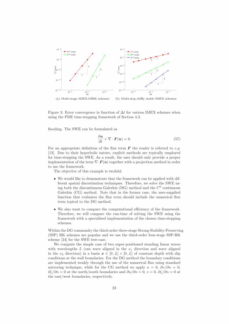
We have applied the time-stepping framework on this equation both formulti-stage and multi-step IMEX time-integration schemes. Therefore, we havesupplied the framework with the three necessary external routines as explainedin Section 4.3.3, i.e. a function that evaluates the linear advection term, aprojection operator and a Helmholtz solver. In order to verify that the frame-work integrates the PDE correctly, we have checked the order of convergence infunction of the time-step ∆t. Fig. 3(a) confirms the correct convergence ratefor the 2nd- and the 3rd-order IMEX-DIRK schemes as respectively presentedin [2, 1] (see also Eq. (74)). In Fig. 3(b), we can observe that the L2 errorconverges according to the expected rate for the multi-step stiffly stable schemesintroduced in Section 5.3 when using the framework.

5.2 Shallow water equations

The shallow water equations (SWE) are frequently used for simulating flows inshallow coastal regions and rivers, for example storm surges, tsunamis and river

22

∆t

L2

error

1

1

3

2

2nd-order

3rd-order

10−5 10−410−3

10−12

10−11

10−10

10−9

10−8

(a) Multi-stage IMEX-DIRK schemes

∆t

L2

error

1

1

1

3

2

1

1st-order

2nd-order

3rd-order

10−510−4 10−3

10−12

10−10

10−8

10−6

10−4

10−2

(b) Multi-step stiffly stable IMEX schemes

Figure 3: Error convergence in function of ∆t for various IMEX schemes whenusing the PDE time-stepping framework of Section 4.3.

flooding. The SWE can be formulated as

∂u

∂t+∇ · F (u) = 0. (57)

For an appropriate definition of the flux term F the reader is referred to e.g.[13]. Due to their hyperbolic nature, explicit methods are typically employedfor time-stepping the SWE. As a result, the user should only provide a properimplementation of the term ∇·F (u) together with a projection method in orderto use the framework.

The objective of this example is twofold:

• We would like to demonstrate that the framework can be applied with dif-ferent spatial discretisation techniques. Therefore, we solve the SWE us-ing both the discontinuous Galerkin (DG) method and the C0 continuousGalerkin (CG) method. Note that in the former case, the user-suppliedfunction that evaluates the flux term should include the numerical fluxterm typical to the DG method.

• We also want to compare the computational efficiency of the framework.Therefore, we will compare the run-time of solving the SWE using theframework with a specialised implementation of the chosen time-steppingschemes.

Within the DG community the third-order three-stage Strong-Stability-Preserving(SSP) RK schemes are popular and we use the third-order four-stage SSP-RKscheme [24] for the SWE test-case.

We compute the simple case of two super-positioned standing linear waveswith wavelengths L (one wave aligned in the x1 direction and wave alignedin the x2 direction) in a basin x ∈ [0 , L] × [0 , L] of constant depth with slipconditions at the wall boundaries. For the DG method the boundary conditionsare implemented weakly through the use of the numerical flux using standardmirroring technique, while for the CG method we apply u = 0, ∂v/∂n = 0,∂ζ/∂n = 0 at the north/south boundaries and ∂u/∂n = 0, v = 0, ∂ζ/∂n = 0 atthe east/west boundaries, respectively.

23

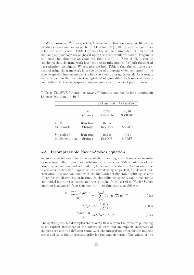
We are using a 3rd order spectral/hp element method on a mesh of 16 quadri-lateral elements and we solve the problem for t ∈ [0 , 100T ] wave where T de-notes the wave period. Table 1 present the required time step, the measuredrun-time and memory usage (based upon the heap profiler Massif of Valgrind’stool suite) for obtaining an error less than 1 × 10−4. First of all, it can beconcluded that the framework has been successfully applied for both the spatialdiscretisation techniques. We can also see from Table 1 that the run-time over-head of using the framework is in the order of a percent when compared to thescheme-specific implementations while the memory usage is equal. As a result,we can conclude that next to the high-level of generality, the framework also iscompetitive with scheme-specific implementations in terms of performance.

Table 1: The SWE for standing waves. Computational results for obtaining anL2 error less than 1× 10−4.

DG method CG method

∆t T/69 T/70L2 error 9.88E-05 9.73E-06

GLM Run-time 16.8 s 13.7 sframework Storage 15.7 MB 8.0 MB

Specialised Run-time 16.7 s 13.5 simplementation Storage 15.7 MB 8.0 MB

5.3 Incompressible Navier-Stokes equation

As an illustrative example of the use of the time-integration framework to solvemore complex fluid dynamics problems, we consider a DNS simulation of thetwo-dimensional flow past a circular cylinder in a free stream. The incompress-ible Navier-Stokes (NS) equations are solved using a spectral/hp element dis-cretisation in space combined with the high-order stiffly stable splitting schemeof [20] for the discretisation in time. In this splitting scheme, each time step issubdivided into three substeps, and the solution of the discretised Navier-Stokesequation is advanced from time-step n− 1 to time-step n as follows:

u−∑Ji

q=1 αqun−q

∆t=−

Je−1∑

q=1

βq [(u · ∇)u]n−q

, (58a)

∇2pn =∇ ·(

u

∆t

)

, (58b)

γ0un − u

∆t=ν∇2un −∇pn. (58c)

The splitting scheme decouples the velocity field u from the pressure p, leadingto an explicit treatment of the advection term and an implicit treatment ofthe pressure and the diffusion term. Ji is the integration order for the implicitterms and Je is the integration order for the explicit terms. The values of the

24

coefficients γ0 , αq and βq of this multi-step IMEX scheme are given in Table 2for different orders. In order to use the PDE time-stepping framework of Section

Table 2: Stiffly stable splitting scheme coefficients

1st-order 2nd-order 3rd-orderγ0 1 3/2 11/6α0 1 2 3α1 0 −1/2 −3/2α2 0 0 1/3β0 1 2 3β1 0 −1 −3β2 0 0 1

4, we first formulate the stiffly stable scheme as a general linear method. Forthe second-order variant for example, this yields

[

AIM AEX U

BIM BEX V

]

=

23 0 4

3 − 13

43 − 2

323 0 4

3 − 13

43 − 2

3

0 0 1 0 0 0

0 1 0 0 0 0

0 0 0 0 1 0

with y[n] =

yn

yn−1

∆tF n

∆tF n−1

.

(59)where the values in the first two rows have been scaled with γ0 compared tothe values in Table 2. Furthermore, we need to properly define the externalfunctions needed for the time-stepping framework:

• For the explicit term, this should be a function f that evaluates the ad-vection term, i.e.

f(u) = − (u · ∇)u. (60)

Because we will follow a pseudo-spectral approach for the advection term,this term should simply be evaluated at the quadrature/collocation points.

• The projection operator to be provided to the system is identical to theone defined in Section 4.3.1.

• For the implicit part of the scheme, a routine that solves the followingproblem is required. Given an arbitrary function f , a scalar λ and atime-level t, find the velocity field u such that

∇2p =∇ · (fλ), (61a)

u− νλ∇2u =f − λ∇p, (61b)

and subject to the appropriate boundary conditions. It can be observedthat this problem involves the consecutive solution of three elliptic prob-lems: a Poisson problem and two (in 2D) scalar Helmholtz problems. Thisroutine can also be used to solve the unsteady Stokes equations.

25

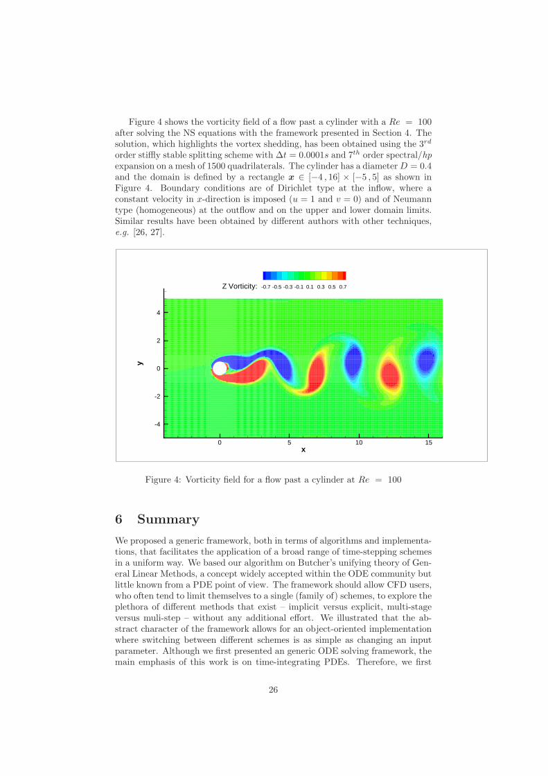
Figure 4 shows the vorticity field of a flow past a cylinder with a Re = 100after solving the NS equations with the framework presented in Section 4. Thesolution, which highlights the vortex shedding, has been obtained using the 3rd

order stiffly stable splitting scheme with ∆t = 0.0001s and 7th order spectral/hpexpansion on a mesh of 1500 quadrilaterals. The cylinder has a diameterD = 0.4and the domain is defined by a rectangle x ∈ [−4 , 16] × [−5 , 5] as shown inFigure 4. Boundary conditions are of Dirichlet type at the inflow, where aconstant velocity in x-direction is imposed (u = 1 and v = 0) and of Neumanntype (homogeneous) at the outflow and on the upper and lower domain limits.Similar results have been obtained by different authors with other techniques,e.g. [26, 27].

x

y

0 5 10 15

-4

-2

0

2

4

Z Vorticity: -0.7 -0.5 -0.3 -0.1 0.1 0.3 0.5 0.7

Figure 4: Vorticity field for a flow past a cylinder at Re = 100

6 Summary

We proposed a generic framework, both in terms of algorithms and implementa-tions, that facilitates the application of a broad range of time-stepping schemesin a uniform way. We based our algorithm on Butcher’s unifying theory of Gen-eral Linear Methods, a concept widely accepted within the ODE community butlittle known from a PDE point of view. The framework should allow CFD users,who often tend to limit themselves to a single (family of) schemes, to explore theplethora of different methods that exist – implicit versus explicit, multi-stageversus muli-step – without any additional effort. We illustrated that the ab-stract character of the framework allows for an object-oriented implementationwhere switching between different schemes is as simple as changing an inputparameter. Although we first presented an generic ODE solving framework, themain emphasis of this work is on time-integrating PDEs. Therefore, we first

26

showed how IMEX schemes – a family of time-stepping schemes popular withinthe CFD community – can be formulated as a General Linear Method. Then wedemonstrated how through some modifications, the framework can be adaptedto accommodate the time-integration of PDEs, characterised by some typicalfeatures such as time-dependent boundary conditions, in a generic and com-putationally efficient way. Overall we believe the paper provides the essentialbuilding blocks for time-integrating PDEs in a unified way. Finally, please notethat even though we mainly followed a finite element procedure for the spatialdiscretisation the presented techniques are general and can be used within afinite volume or finite difference context.

Acknowledgment

The authors would like to acknowledge the insightful input of Professor RaySpiteri of the University of Saskatchewan. SJS would like to acknowledge thesupport under an EPSRC Advance Research Fellowship, SC would like to ac-knowledge support from the CardioMath initiative of the Institute of Mathemat-ical Science at Imperial College London, and RMK would like to acknowledgesupport under the Leverhulme Foundation Trust.

References

[1] U.M. Ascher, S.J. Ruuth, and R.J. Spiteri. Implicit–explicit Runge–Kuttamethods for time-dependent partial differential equations. Appl. Numer.Math., 25(2–3):151–167, 1997.

[2] U.M. Ascher, S.J. Ruuth, and B.T.R. Wetton. Implicit-explicit methodsfor time-dependent partial differential equations. SIAM J. Numer. Anal.,32(3):797–823, 1995.

[3] K. Burrage and J. C. Butcher. Non-linear stability of a general class ofdifferential equation methods. BIT, 20:185–203, 1980.

[4] J. C. Butcher. The Numerical Analysis of Ordinary Differential Equations:Runge-Kutta and General Linear Methods. Wiley, Chichester, 1987.

[5] J. C. Butcher. General linear methods. Acta Numerica, 15:157–256, 2006.

[6] J.C. Butcher. On the convergence of numerical solutions of ordinary dif-ferential equations. Math. Comp., pages 1–10, 1966.

[7] J.C. Butcher. Diagonally-implicit multi-stage integration methods. Appl.Numer. Math., 11:347–363, 1993.

[8] J.C. Butcher. An introduction to DIMSIMs. Math. Appl. Comput., 14:59–72, 1995.

[9] J.C. Butcher. An introduction to Almost Runge-Kutta methods. Appl.Numer. Math., 24:331–342, 1997.

[10] J.C. Butcher, P. Chartier, and Z. Jackiewicz. Experiments with a variable-order type 1 DIMSIM code. Numer. Algorithms, 22:237–261, 1999.

27

[11] J. Donea, S. Giuliani, H. Laval, and L. Quartapelle. Time-accurate solutionof advection-diffusion problems by finite elements. Comput. Methods Appl.Mech. Engrg., 45(1-3):123–145, 1984.

[12] J. Donelson and E. Hansen. Cyclic composite multistep predictor-correctormethods. SIAM Journal for Numerical Analysis, 8(1):137–157, 1971.

[13] C. Eskilsson and S. J. Sherwin. A triangular spectral/hp discontinuousgalerkin method for modelling 2d shallow water equations. Int. J. Numer.Meth. Fluids, 45:605–623, 2004.

[14] D. Gottlieb and S. A. Orszag. Numerical analysis of spectral methods:theory and applications. CBMS-NSF. Society for Industrial and AppliedMathematics, Philadelphia, 1977.

[15] Z. Jackiewicz. Implementation of DIMSIMs for stiff differential equations.Appl. Numer. Math., 42:251–267, 2002.

[16] Z. Jackiewicz. Construction and implementation of general linear methodsfor ordinary differential equations. A review. J. Sci. Comp., 25:29–49, 2005.

[17] Z. Jackiewicz. General Linear Methods for Ordinary Differential Equations.Wiley, 2009.

[18] Z. Jackiewicz and S. Tracogna. A general class of two-step Runge-Kuttamethods for ordinary differential equations. SIAM J. Num. Anal., 32:1390–1427, 1995.

[19] A. Kanevsky, M.H. Carpenter, D. Gottlieb, and J.S. Hesthaven. Applica-tion of implicit-explicit high order Runge-Kutta methods to discontinuous-galerkin schemes. J. Comp. Phys., 225:1753–1781, 2007.

[20] G. E. Karniadakis, M. Israeli, and S. A. Orszag. High-order splittingmethods for the incompressible navier-stokes equations. J. Comput. Phys.,97:414–443, 1991.

[21] G. E. Karniadakis and S. J. Sherwin. Spectral/hp Element Methods forCFD. Oxford University Press, second edition edition, 2005.

[22] B. J. Noye and H. H. Tan. Finite difference methods for solving the two-dimensional advection-diffusion equation. Int. J. Numer. Meth. Fluids,9(1):75–89, 1989.

[23] N. Rattenbury. Almost Runge-Kutta methods for stiff and non-stiff prob-lems. PhD thesis, The University of Auckland, 2005.

[24] S. J. Ruuth and R. J. Spiteri. High-order strong-stability-preserving Runge-Kutta methods with downwind-biased spatial discretizations. Siam J. Nu-mer. Anal., 42(3):974–996, 2004.

[25] W. E. Schiesser. The Numerical Method of Lines: Integration of PartialDifferential Equations. Academic Press, San Diego, 1991.

[26] C.C.S. Song and M. Yuan. Simulation of vortex-shedding flow about acircular cylinder at high Reynolds numbers. J. Fluids Eng., 112, 1990.

28

[27] B. Souza Carmo. On Wake Interference in the Flow around Two CircularCylinders: Direct Stability Analysis and Flow-Induced Vibrations. PhDthesis, Department of Aeronautics, Imperial College London, 2009.

[28] J. vanWieren. Using diagonally implicit multistage integrations methodsfor solving ordinary differential equations. part 1: Introduction and explicitmethods. NAWCWPNS TP 8340, Naval Air Warfare Center WeaponsDivision, 1997.

[29] J. vanWieren. Using diagonally implicit multistage integrations methods forsolving ordinary differential equations. part 2: Implicit methods. NAWCW-PNS TP 8356, Naval Air Warfare Center Weapons Division, 1997.

[30] W. Wright. General Linear Methods with Inherent Runge-Kutta Stability.PhD thesis, University of Auckland, 2002.

A Coefficients of GLM methods

A.1 Common multi-stage methods

Since multi-stage methods consist only of a single step with many stages, theycan be represented as a general linear method with r = 1. It is sufficient towrite U = [ 1 1 · · · 1 ]⊤, V = [1] and to set the coefficient matrices A and Bto the matrix A and the single row b⊤ of the corresponding Butcher tableau [5]respectively. For example, the classic fourth-order Runge-Kutta method withButcher tableau

c A

b⊤=

012

12

12 0 1

2

1 0 0 116

13

13

16

, (62)

has the following GLM representation

[

A UB V

]

=

0 0 0 0 112 0 0 0 10 1

2 0 0 10 0 1 0 116

13

13

16 1

. (63)

A.2 Common multi-step methods

In contrast to multi-stage methods, multi-step methods have a single stage,but the solution at the new time-level is computed as a linear combination ofinformation at the r previous time-levels. Linear multi-step methods can beformulated to satisfy the relation

yn =

r∑

i=1

αiyn−i +∆t

r∑

i=0

βiF n−i. (64)

29

This corresponds to the general linear method with input and output

y[n−1] =

yn−1

yn−2...

yn−r

∆tF n−1

∆tF n−2

...∆tF n−r

, y[n] =

yn

yn−1...

yn−r+1

∆tF n

∆tF n−1

...∆tF n−r+1

, (65)

and the partitioned coefficient matrix

[

A UB V

]

=

β0 α1 α2 · · · αr−1 αr β1 β2 · · · βr−1 βr

β0 α1 α2 · · · αr−1 αr β1 β2 · · · βr−1 βr

0 1 0 · · · 0 0 0 0 · · · 0 00 0 1 · · · 0 0 0 0 · · · 0 0...

......

......

......

......

0 0 0 · · · 1 0 0 0 · · · 0 01 0 0 · · · 0 0 0 0 · · · 0 00 0 0 · · · 0 0 1 0 · · · 0 00 0 0 · · · 0 0 0 1 · · · 0 0...

......

......

......

......

0 0 0 · · · 0 0 0 0 · · · 1 0

.

(66)Note that in the vectors and matrices above, the solid lines denote the demar-cation of the matrices A, B, U and V whereas the dotted lines merely help tohighlight the typical structure of a linear multi-step method. As an exampleof a multi-step scheme consider the well-known third-order Adams-Bashforthscheme

yn = yn−1 +∆t

(

23

12f(yn−1)−

4

3f(yn−2) +

5

12f(yn−3)

)

, (67)

which has the following GLM representation

[

A UB V

]

=

0 1 2312 − 4

3512

0 1 2312 − 4

3512

1 0 0 0 0

0 0 1 0 0

0 0 0 1 0

. (68)

A.3 Beyond common multi-step or multi-stage methods

The general linear methods framework also encompasses methods that do notfit under the conventional Runge-Kutta or linear multi-step headings. Thisincludes, for example, the cyclic composite method of [12]. In addition, thegeneral linear structure of the GLM in itself gave rise to the development of

30

new numerical methods. An example of one such class of methods is the class ofAlmost Runge-Kutta Methods [9]. To appreciate its typical combined multi-stagemulti-step character consider the following third-order scheme due to [23]:

[

A UB V

]

=

0 0 0 1 13

118

12 0 0 1 1

6118

0 34 0 1 1

4 0

0 34 0 1 1

4 0

0 0 1 0 0 0

3 − 3 2 0 − 2 0

. (69)

A.4 Common implicit-explicit methods

The first-order Backward Euler/Forward Euler IMEX scheme,

yn = yn−1 +∆t(

g(yn) + f(yn−1))

, (70)

can be written as a general linear method as

[

AIM AEX U

BIM BEX V

]

=

1 0 1 1

1 0 1 1

0 1 0 0

with y[n] =

[

yn

∆tF n

]

.

(71)The second-order Crank-Nicholson/Adams-Bashforth linear multi-step scheme,

yn = yn−1 +∆t

(

1

2g(yn) +

1

2g(yn−1) +

3

2f(yn−1)−

1

2f(yn−1)

)

, (72)

can be represented as

[

AIM AEX U

BIM BEX V

]

=

12 0 1 1

232 − 1

212 0 1 1

232 − 1

2

1 0 0 0 0 0

0 1 0 0 0 0

0 0 0 0 1 0

with y[n] =

yn

∆tGn

∆tF n

∆tF n−1

.

(73)The third-order (2, 3, 3) IMEX Runge-Kutta scheme (see [1]) is represented bythe partitioned coefficient matrix where γ = (3 +

√3)/6:

[

AIM AEX U

BIM BEX V

]

=

0 0 0 0 0 0 1

0 γ 0 γ 0 0 1

0 1− 2γ γ γ − 1 2(1− γ) 0 1

0 12

12 0 1

212 1

.

(74)

31