A Generalized Linear Model for Binomial Response Data

A Generalized Linear Model

for Binomial Response Data

Copyright c©2017 Dan Nettleton (Iowa State University) Statistics 510 1 / 46

Now suppose that instead of a Bernoulli response, we

have a binomial response for each unit in an

experiment or an observational study.

As an example, consider the trout data set discussed

on page 669 of The Statistical Sleuth, 3rd edition, by

Ramsey and Schafer.

Five doses of toxic substance were assigned to a

total of 20 fish tanks using a completely randomized

design with four tanks per dose.

For each tank, the total number of fish and the

number of fish that developed liver tumors were

recorded.


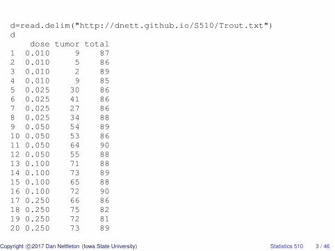
d=read.delim("http://dnett.github.io/S510/Trout.txt")d

dose tumor total1 0.010 9 872 0.010 5 863 0.010 2 894 0.010 9 855 0.025 30 866 0.025 41 867 0.025 27 868 0.025 34 889 0.050 54 8910 0.050 53 8611 0.050 64 9012 0.050 55 8813 0.100 71 8814 0.100 73 8915 0.100 65 8816 0.100 72 9017 0.250 66 8618 0.250 75 8219 0.250 72 8120 0.250 73 89


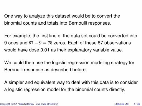
One way to analyze this dataset would be to convert thebinomial counts and totals into Bernoulli responses.

For example, the first line of the data set could be converted into9 ones and 87− 9 = 78 zeros. Each of these 87 observationswould have dose 0.01 as their explanatory variable value.

We could then use the logistic regression modeling strategy forBernoulli response as described before.

A simpler and equivalent way to deal with this data is to considera logistic regression model for the binomial counts directly.


A Logistic Regression Model for Binomial Count Data

For all i = 1, ..., n,

yi ∼ binomial(mi, πi),

where mi is a known number of trials for observation i,

πi =exp(x′iβ)

1 + exp(x′iβ),

and y1, ..., yn are independent.


The Binomial Distribution

Recall that for yi ∼ binomial(mi, πi), the probability

mass function of yi is

P(yi = y) =

{ (miy

)πy

i (1− πi)mi−y for y ∈ {0, ...,mi}

0 otherwise,

E(yi) = miπi, and Var(yi) = miπi(1− πi).


The Binomial Log Likelihood

The binomial log likelihood function is

`(β | y) =n∑

i=1

[yi log

(πi

1− πi

)+ mi log(1− πi)

]+ constant

=n∑

i=1

[yi x′iβ − mi log(1 + exp{−x′iβ})]

+ constant.


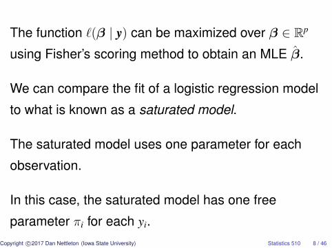
The function `(β | y) can be maximized over β ∈ Rp

using Fisher’s scoring method to obtain an MLE β.

We can compare the fit of a logistic regression model

to what is known as a saturated model.

The saturated model uses one parameter for each

observation.

In this case, the saturated model has one free

parameter πi for each yi.Copyright c©2017 Dan Nettleton (Iowa State University) Statistics 510 8 / 46

Logistic Regression Model

yi ∼ binomial(mi, πi)

y1, ..., yn independent

πi =exp(x′iβ)

1+exp(x′iβ)

for some β ∈ Rp

p parameters

Saturated Model

yi ∼ binomial(mi, πi)

y1, ..., yn independent

πi ∈ [0, 1] for i = 1, ..., n

with no other restrictions

n parameters


For all i = 1, . . . , n,

the MLE of πi under the logistic regression model is

πi =exp(x′iβ)

1 + exp(x′iβ),

and the MLE of πi under the saturated model is

yi/mi.


Then the likelihood ratio statistic for testing the logistic

regression model as the reduced model vs. the

saturated model as the full model is

2n∑

i=1

[yi log

(yi/mi

πi

)+ (mi − yi) log

(1− yi/mi

1− πi

)].


This statistic is sometimes called

the Deviance Statistic,

the Residual Deviance,

or just the the Deviance.


A Lack-of-Fit Test

When n is suitably large and/or m1, . . . ,mn are each

suitably large, the Deviance Statistic is approximately

χ2n−p if the logistic regression model is correct.

Thus, the Deviance Statistic can be compared to the

χ2n−p distribution to test for lack of fit of the logistic

regression model.


Deviance Residuals

The term

di ≡ sign(yi/mi − πi)

√2[

yi log

(yi

miπi

)+ (mi − yi) log

(mi − yi

mi − miπi

)]

is called a deviance residual.

Note that the residual deviance statistic is the sum of

the squared deviance residuals (∑n

i=1 d2i ).


Pearson’s Chi-Square Statistic

Another lack of fit statistic that is approximately χ2n−p

under the null is Pearson’s Chi-Square Statistic:

X2 =n∑

i=1

yi − E(yi)√Var(yi)

2

=n∑

i=1

(yi − miπi√miπi(1− πi)

)2

.


Pearson Residuals

The term

ri =yi − miπi√miπi(1− πi)

is known as a Pearson residual.

Note that the Pearson statistic is the sum of the

squared Pearson residuals (∑n

i=1 r2i ).


Residual Diagnostics

For large mi values, both di and ri should be

approximately distributed as standard normal random

variables if the logistic regression model is correct.

Thus, either set of residuals can be used to diagnose

problems with model fit by, e.g., identifying outlying

observations.


Strategy for Inference

1 Find the MLE for β using the method of Fisher

Scoring, which results in an iterative weighted

least squares approach.

2 Obtain an estimate of the inverse Fisher

information matrix that can be used for Wald type

inference concerning β and/or conduct likelihood

ratio based inference of reduced vs. full models.


#Let's plot observed tumor proportions #for each tank. plot(d$dose,d$tumor/d$total,col=4,pch=19, xlab="Dose", ylab="Proportion of Fish with Tumor")

19

#Let's fit a logistic regression model #dose is a quantitative explanatory variable. o=glm(cbind(tumor,total-tumor)~dose, family=binomial(link=logit), data=d) summary(o) Call: glm(formula = cbind(tumor, total - tumor) ~ dose, family = binomial(link = logit), data = d) Deviance Residuals: Min 1Q Median 3Q Max -7.3577 -4.0473 -0.1515 2.9109 4.7729

21

Coefficients: Estimate Std. Error z value Pr(>|z|) (Intercept) -0.86705 0.07673 -11.30 <2e-16 *** dose 14.33377 0.93695 15.30 <2e-16 *** (Dispersion parameter for binomial family taken to be 1) Null deviance: 667.20 on 19 degrees of freedom Residual deviance: 277.05 on 18 degrees of freedom AIC: 368.44 Number of Fisher Scoring iterations: 5

22

#Let's plot the fitted curve. b=coef(o) u=seq(0,.25,by=0.001) xb=b[1]+u*b[2] pihat=1/(1+exp(-xb)) lines(u,pihat,col=2,lwd=1.3)

23

#Let's use a reduced versus full model #likelihood ratio test to test for #lack of fit relative to the #saturated model. 1-pchisq(deviance(o),df.residual(o)) [1] 0 #We could try adding higher-order #polynomial terms, but let's just #skip right to the model with dose #as a categorical variable.

25

d$dosef=gl(5,4) d dose tumor total dosef 1 0.010 9 87 1 2 0.010 5 86 1 3 0.010 2 89 1 4 0.010 9 85 1 5 0.025 30 86 2 6 0.025 41 86 2 7 0.025 27 86 2 8 0.025 34 88 2 9 0.050 54 89 3 10 0.050 53 86 3 11 0.050 64 90 3 12 0.050 55 88 3 13 0.100 71 88 4 14 0.100 73 89 4 15 0.100 65 88 4 16 0.100 72 90 4 17 0.250 66 86 5 18 0.250 75 82 5 19 0.250 72 81 5 20 0.250 73 89 5

26

o=glm(cbind(tumor,total-tumor)~dosef, family=binomial(link=logit), data=d) summary(o) Call: glm(formula = cbind(tumor, total - tumor) ~ dosef, family = binomial(link = logit), data = d) Deviance Residuals: Min 1Q Median 3Q Max -2.0966 -0.6564 -0.1015 1.0793 1.8513

27

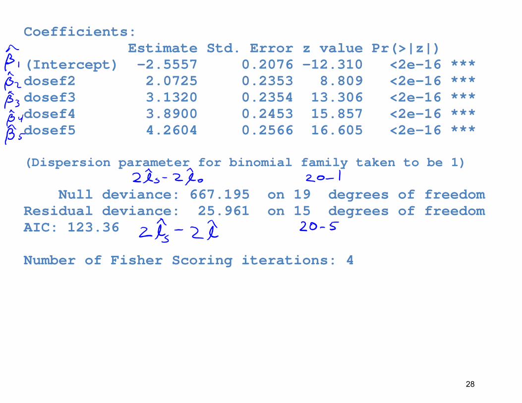
Coefficients: Estimate Std. Error z value Pr(>|z|) (Intercept) -2.5557 0.2076 -12.310 <2e-16 *** dosef2 2.0725 0.2353 8.809 <2e-16 *** dosef3 3.1320 0.2354 13.306 <2e-16 *** dosef4 3.8900 0.2453 15.857 <2e-16 *** dosef5 4.2604 0.2566 16.605 <2e-16 *** (Dispersion parameter for binomial family taken to be 1) Null deviance: 667.195 on 19 degrees of freedom Residual deviance: 25.961 on 15 degrees of freedom AIC: 123.36 Number of Fisher Scoring iterations: 4

28

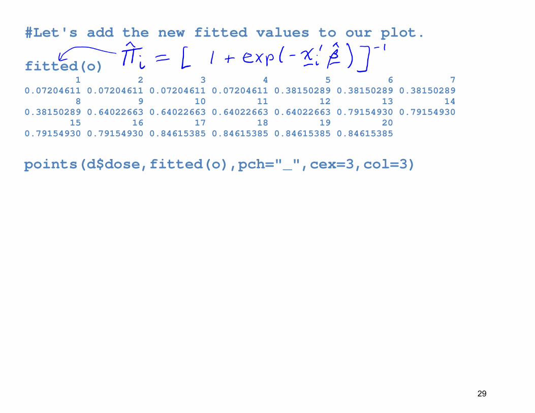
#Let's add the new fitted values to our plot. fitted(o) 1 2 3 4 5 6 7 0.07204611 0.07204611 0.07204611 0.07204611 0.38150289 0.38150289 0.38150289 8 9 10 11 12 13 14 0.38150289 0.64022663 0.64022663 0.64022663 0.64022663 0.79154930 0.79154930 15 16 17 18 19 20 0.79154930 0.79154930 0.84615385 0.84615385 0.84615385 0.84615385

points(d$dose,fitted(o),pch="_",cex=3,col=3)

29

#The fit looks good, but let's formally #test for lack of fit. 1-pchisq(deviance(o),df.residual(o)) [1] 0.03843272 #There is still a significant lack of fit #when comparing to the saturated model. #The problem is over dispersion, otherwise #known in this case as extra binomial variation.

31

Overdispersion

In the Generalized Linear Models framework, its often

the case that Var(yi) is a function of E(yi).

That is the case for logistic regression where

Var(yi) = miπi(1− πi) = miπi −(miπi)

2

mi

= E(yi)− [E(yi)]2/mi.


Thus, when we fit a logistic regression model and

obtain estimates of the mean of the response, we get

estimates of the variance of the response as well.

If the variability of our response is greater than we

should expect based on our estimates of the mean,

we say that there is overdispersion.


If either the Deviance Statistic or the Pearson Chi

Square Statistic suggests a lack of fit that cannot be

explained by other reasons (e.g., poor model for the

mean or a few extreme outliers), overdispersion may

be the problem.


Quasi-Likelihood Inference

If there is overdispersion, a quasi-likelihood approach

may be used.

In the binomial case, we make all the same

assumptions as before except that we assume

Var(yi) = φ mi πi(1− πi)

for some unknown dispersion parameter φ > 1.


The dispersion parameter φ can be estimated by

φ =

∑ni=1 d2

i

n− p

or

φ =

n∑i=1

r2i

n− p.


All analyses are as before except that

1 The estimated variance of β is multiplied by φ.

2 For Wald type inferences, the standard normal null

distribution is replaced by t with n− p degrees of

freedom.

3 Any test statistic T that was assumed χ2q under H0

is replaced with T/(qφ) and compared to an F

distribution with q and n− p degrees of freedom.Copyright c©2017 Dan Nettleton (Iowa State University) Statistics 510 38 / 46

These changes to the inference strategy in the

presence of overdispersion are analogous to the

changes that would take place in normal theory

Gauss-Markov linear model analysis if we switched

from assuming σ2 were known to be 1 to assuming σ2

were unknown and estimating it with MSE.

(Here φ is like σ2 and φ is like MSE.)


Whether there is overdispersion or not, all the usual

ways of conducting generalized linear models

inference are approximate except for the special case

of normal theory linear models.


#Let's estimate the dispersion parameter. phihat=deviance(o)/df.residual(o) phihat [1] 1.730745 #We can obtain the same estimate by using #the deviance residuals. di=residuals(o,type="deviance") sum(di^2)/df.residual(o) [1] 1.730745 #We can obtain an alternative estimate by #using the Pearson residuals. ri=residuals(o,type="pearson") phihat=sum(ri^2)/df.residual(o) phihat

41

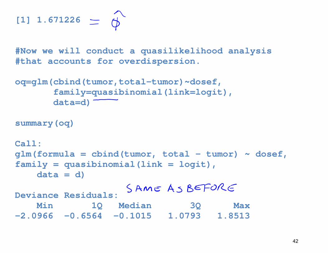
[1] 1.671226 #Now we will conduct a quasilikelihood analysis #that accounts for overdispersion. oq=glm(cbind(tumor,total-tumor)~dosef, family=quasibinomial(link=logit), data=d) summary(oq) Call: glm(formula = cbind(tumor, total - tumor) ~ dosef, family = quasibinomial(link = logit), data = d) Deviance Residuals: Min 1Q Median 3Q Max -2.0966 -0.6564 -0.1015 1.0793 1.8513

42

Coefficients: Estimate Std. Error t value Pr(>|t|) (Intercept) -2.5557 0.2684 -9.522 9.48e-08 *** dosef2 2.0725 0.3042 6.814 5.85e-06 *** dosef3 3.1320 0.3043 10.293 3.41e-08 *** dosef4 3.8900 0.3171 12.266 3.20e-09 *** dosef5 4.2604 0.3317 12.844 1.70e-09 *** (Dispersion parameter for quasibinomial family taken to be 1.671232) Null deviance: 667.195 on 19 degrees of freedom Residual deviance: 25.961 on 15 degrees of freedom AIC: NA Number of Fisher Scoring iterations: 4

43

#Test for the effect of dose on the response. drop1(oq,test="F") Single term deletions Model: cbind(tumor, total - tumor) ~ dosef Df Deviance F value Pr(F) <none> 25.96 dosef 4 667.20 92.624 2.187e-10 *** #The F value is computed as #[(667.20-25.96)/(19-15)]/(25.96/15) #This computation is analogous to #[(SSEr-SSEf)/(DFr-DFf)]/(SSEf/DFf) #where deviance is like SSE. #There is strong evidence that #the probability of tumor formation #is different for different doses #of the toxicant.

44

#Let's test for a difference between #the top two doses. b=coef(oq) b (Intercept) dosef2 dosef3 dosef4 dosef5 -2.555676 2.072502 3.132024 3.889965 4.260424 v=vcov(oq) v (Intercept) dosef2 dosef3 dosef4 dosef5 (Intercept) 0.0720386 -0.07203860 -0.07203860 -0.0720386 -0.0720386 dosef2 -0.0720386 0.09250893 0.07203860 0.0720386 0.0720386 dosef3 -0.0720386 0.07203860 0.09259273 0.0720386 0.0720386 dosef4 -0.0720386 0.07203860 0.07203860 0.1005702 0.0720386 dosef5 -0.0720386 0.07203860 0.07203860 0.0720386 0.1100211

45

se=sqrt(t(c(0,0,0,-1,1))%*%v%*%c(0,0,0,-1,1)) tstat=(b[5]-b[4])/se pval=2*(1-pt(abs(tstat),df.residual(oq))) pval 0.1714103

46

A Generalized Linear Model for Binomial Response Data

Documents

Transcript of A Generalized Linear Model for Binomial Response Data