A General Framework Integrating Techniques for Scheduling under...
144
Serial Number: 2297 A General Framework Integrating Techniques for Scheduling under Uncertainty by Julien Bidot Automated-production engineer, Ecole Nationale d’Ingénieurs de Tarbes A dissertation presented at Ecole Nationale d’Ingénieurs de Tarbes in conformity with the requirements for the degree of Doctor of Philosophy of Institut National Polytechnique de Toulouse, France Specialty: Industrial Systems 28 November 2005 Submitted to the following committee members: Chairman: Gérard Verfaillie ONERA, France Reviewer: Amedeo Cesta I.S.T.C.–C.N.R., Italy Reviewer: Erik L. Demeulemeester Katholieke Universiteit Leuven, Belgium Reviewer and invited member: Eric Sanlaville LIMOS–Université Blaise Pascal, France Advisor: Bernard Grabot L.G.P.–ENIT, France Academical mentor: Thierry Vidal L.G.P.–ENIT, France Industrial mentor: Philippe Laborie ILOG S.A., France Invited member: J. Christopher Beck University of Toronto, Canada
Transcript of A General Framework Integrating Techniques for Scheduling under...

Serial Number: 2297
A General Framework IntegratingTechniques for Scheduling under Uncertainty
by
Julien BidotAutomated-production engineer, Ecole Nationale d’Ingénieurs de Tarbes
A dissertation presented at Ecole Nationale d’Ingénieurs de Tarbesin conformity with the requirements
for the degree of Doctor of Philosophyof Institut National Polytechnique de Toulouse, France
Specialty: Industrial Systems
28 November 2005
Submitted to the following committee members:
Chairman: Gérard Verfaillie ONERA, FranceReviewer: Amedeo Cesta I.S.T.C.–C.N.R., ItalyReviewer: Erik L. Demeulemeester Katholieke Universiteit Leuven, BelgiumReviewer and invited member: Eric Sanlaville LIMOS–Université Blaise Pascal, FranceAdvisor: Bernard Grabot L.G.P.–ENIT, FranceAcademical mentor: Thierry Vidal L.G.P.–ENIT, FranceIndustrial mentor: Philippe Laborie ILOG S.A., FranceInvited member: J. Christopher Beck University of Toronto, Canada


Acknowledgments
Many people have helped me directly or indirectly to achieve this dissertation, making itbetter than it otherwise would have been.
Thanks to Philippe Laborie for his guidance, insight, kindness, and availability. It hasbeen very pleasant to work with him at ILOG. In particular, he has been of great helpto implement algorithms.
Thanks to Thierry Vidal for his constant support, helpful suggestions, and kindness.He has always trusted me and I have been quite free to organize as I have wanted. I haveappreciated this even if freedom has sometimes meant complex decisions to make.
Thanks to Chris Beck for guiding me and giving me advices all along my Ph.D. thesiseven if he has not always been physically close to me. He has been a precious mentorduring my first six months at ILOG and during my visit at Cork Constraint ComputationCentre (4C).
Thanks to Jérôme Rogerie for his participation in the achievement of this researchwork, in particular, during our investigation of potential industrial applications.
I thank Amedeo Cesta, Erik Demeulemeester, and Eric Sanlaville for reviewing mydissertation given a short-time period. I also thank Gérard Verfaillie for taking part ofmy jury.
Thanks to my advisor, Bernard Grabot, for his sustained encouragement. I also thankthe members of the research group “Production Automatisée” for helping me during thedifferent time periods I have been working in Laboratoire Génie de Production (L.G.P.).
Thanks to Daniel Noyes and the administrative staff of L.G.P. for having hosted meseveral times during my Ph.D. thesis.
Thanks to Eugene Freuder and all the members of 4C. They have been hosting mefor three months providing me a stimulating environment contributing to the outcome ofmy dissertation.
Thanks to Jeremy Frank, my mentor at the CP’03 doctoral program who made relevantremarks about my work. Thanks also to Jim Blythe who was my mentor at the ICAPS’03doctoral consortium.
Thanks to Hassan Aït-Kaci, Emilie Danna, Bruno De Backer, Vincent Furnon, DanielGodard, Emmanuel Guéré, Pascal Massimino, Claude Le Pape, Pierre Lopez, Wim Nui-jten, Laurent Perron, Jean-Charles Régin, Francis Sourd, the members of the French re-search group “flexibilité” of GOThA (Groupe de recherche sur l’Ordonnancement Théoriqueet Appliqué), and many others for their help and wealthy ideas.
Special thanks go to the members of my family for their financial, intellectual, andemotional support throughout this long and challenging process. Last and not least, Ithank my girlfriend, Hélène, for her love, patience, and encouragement.
Encore une dernière fois, merci à toutes et à tous.
iii


Contents
Acknowledgments iii
List of Tables ix
List of Figures xi
Introduction 1
1 State of the Art 51.1 What We Do Not Review . . . . . . . . . . . . . . . . . . . . . . . . . . . 51.2 Deterministic Domains . . . . . . . . . . . . . . . . . . . . . . . . . . . . . 5
1.2.1 Task Planning . . . . . . . . . . . . . . . . . . . . . . . . . . . . . . 61.2.2 Scheduling . . . . . . . . . . . . . . . . . . . . . . . . . . . . . . . . 71.2.3 Bridging the Gap Between Task Planning and Scheduling . . . . . . 81.2.4 Models . . . . . . . . . . . . . . . . . . . . . . . . . . . . . . . . . . 91.2.5 Optimization . . . . . . . . . . . . . . . . . . . . . . . . . . . . . . 11
1.3 Non-deterministic Domains . . . . . . . . . . . . . . . . . . . . . . . . . . . 111.3.1 Uncertainty Sources . . . . . . . . . . . . . . . . . . . . . . . . . . 111.3.2 Definitions . . . . . . . . . . . . . . . . . . . . . . . . . . . . . . . . 121.3.3 Uncertainty Models . . . . . . . . . . . . . . . . . . . . . . . . . . . 151.3.4 Temporal Extensions of CSPs . . . . . . . . . . . . . . . . . . . . . 241.3.5 Task Planning under Uncertainty . . . . . . . . . . . . . . . . . . . 251.3.6 Scheduling under Uncertainty . . . . . . . . . . . . . . . . . . . . . 27
1.4 Summary and General Comments . . . . . . . . . . . . . . . . . . . . . . . 35
2 General Framework 372.1 Definitions and Discussion . . . . . . . . . . . . . . . . . . . . . . . . . . . 372.2 Revision Techniques . . . . . . . . . . . . . . . . . . . . . . . . . . . . . . 40
2.2.1 Generalities . . . . . . . . . . . . . . . . . . . . . . . . . . . . . . . 402.2.2 Examples of Revision Techniques in Task Planning and Scheduling 422.2.3 Discussion . . . . . . . . . . . . . . . . . . . . . . . . . . . . . . . . 42
2.3 Proactive Techniques . . . . . . . . . . . . . . . . . . . . . . . . . . . . . . 422.3.1 Generalities . . . . . . . . . . . . . . . . . . . . . . . . . . . . . . . 432.3.2 Examples of Proactive Techniques in Task Planning and Scheduling 442.3.3 Discussion . . . . . . . . . . . . . . . . . . . . . . . . . . . . . . . . 46
2.4 Progressive Techniques . . . . . . . . . . . . . . . . . . . . . . . . . . . . . 462.4.1 Generalities . . . . . . . . . . . . . . . . . . . . . . . . . . . . . . . 462.4.2 Examples of Progressive Techniques in Task Planning and Scheduling 48
v

vi CONTENTS
2.4.3 Discussion . . . . . . . . . . . . . . . . . . . . . . . . . . . . . . . . 492.5 Mixed Techniques . . . . . . . . . . . . . . . . . . . . . . . . . . . . . . . . 49
2.5.1 Generalities . . . . . . . . . . . . . . . . . . . . . . . . . . . . . . . 492.5.2 Examples of Mixed Techniques in Task Planning and Scheduling . . 52
2.6 Summary and General Comments . . . . . . . . . . . . . . . . . . . . . . . 53
3 Application Domain 553.1 Project Management and Project Scheduling . . . . . . . . . . . . . . . . . 553.2 Construction of Dams . . . . . . . . . . . . . . . . . . . . . . . . . . . . . 56
3.2.1 General Description . . . . . . . . . . . . . . . . . . . . . . . . . . . 563.2.2 Uncertainty Sources . . . . . . . . . . . . . . . . . . . . . . . . . . 573.2.3 An Illustrative Example . . . . . . . . . . . . . . . . . . . . . . . . 57
3.3 General Comments . . . . . . . . . . . . . . . . . . . . . . . . . . . . . . . 57
4 Theoretical Model 614.1 Model Expressivity . . . . . . . . . . . . . . . . . . . . . . . . . . . . . . . 614.2 Definitions . . . . . . . . . . . . . . . . . . . . . . . . . . . . . . . . . . . . 64
4.2.1 Scheduling Problem and Schedule Model . . . . . . . . . . . . . . . 644.2.2 Generation and Execution Model . . . . . . . . . . . . . . . . . . . 69
4.3 Schedule Generation and Execution . . . . . . . . . . . . . . . . . . . . . . 724.4 A Toy Example . . . . . . . . . . . . . . . . . . . . . . . . . . . . . . . . . 754.5 Summary and General Comments . . . . . . . . . . . . . . . . . . . . . . . 79
5 Experimental System 815.1 Scheduling Problem . . . . . . . . . . . . . . . . . . . . . . . . . . . . . . . 81
5.1.1 Costs . . . . . . . . . . . . . . . . . . . . . . . . . . . . . . . . . . . 825.2 Architecture . . . . . . . . . . . . . . . . . . . . . . . . . . . . . . . . . . . 83
5.2.1 Solver . . . . . . . . . . . . . . . . . . . . . . . . . . . . . . . . . . 835.2.2 Controller . . . . . . . . . . . . . . . . . . . . . . . . . . . . . . . . 845.2.3 World Simulator . . . . . . . . . . . . . . . . . . . . . . . . . . . . 855.2.4 Resolution Techniques . . . . . . . . . . . . . . . . . . . . . . . . . 855.2.5 Experimental Parameters and Indicators . . . . . . . . . . . . . . . 89
5.3 Revision-Proactive Approach . . . . . . . . . . . . . . . . . . . . . . . . . . 915.3.1 Revision Approach . . . . . . . . . . . . . . . . . . . . . . . . . . . 915.3.2 Proactive Approach . . . . . . . . . . . . . . . . . . . . . . . . . . . 925.3.3 Experimental Studies . . . . . . . . . . . . . . . . . . . . . . . . . . 92
5.4 Progressive-Proactive Approach . . . . . . . . . . . . . . . . . . . . . . . . 995.4.1 When to Try Extending the Current Partial Flexible Schedule? . . 1005.4.2 How to Select the Subset of Operations to Be Allocated and Ordered?1015.4.3 How to Allocate and Order the Subset of Operations? . . . . . . . . 105
5.5 Discussion . . . . . . . . . . . . . . . . . . . . . . . . . . . . . . . . . . . . 1065.6 Summary and General Comments . . . . . . . . . . . . . . . . . . . . . . . 107
6 Future Work 1096.1 Prototype . . . . . . . . . . . . . . . . . . . . . . . . . . . . . . . . . . . . 109
6.1.1 Experimental Studies . . . . . . . . . . . . . . . . . . . . . . . . . . 1096.1.2 Extensions . . . . . . . . . . . . . . . . . . . . . . . . . . . . . . . . 110
6.2 Theoretical Model . . . . . . . . . . . . . . . . . . . . . . . . . . . . . . . . 111

CONTENTS vii
Conclusions 113
Bibliography 115
Index 129


List of Tables
1.1 Off-line/On-line reasoning. . . . . . . . . . . . . . . . . . . . . . . . . . . . 14
2.1 The basic parameters of a progressive approach. . . . . . . . . . . . . . . . 482.2 The properties of each family of solution-generation techniques. . . . . . . 52
ix


List of Figures
1.1 A toy example of a task-planning problem. . . . . . . . . . . . . . . . . . . 71.2 A toy example of a job-shop scheduling problem. . . . . . . . . . . . . . . . 81.3 A toy example of an optimal job-shop scheduling solution. . . . . . . . . . 81.4 Generation and execution in the ideal world. . . . . . . . . . . . . . . . . . 151.5 (a) A Bayesian network and (b) a conditional probability matrix charac-
terizing the causal relation. . . . . . . . . . . . . . . . . . . . . . . . . . . . 171.6 A possibility function of the concept “young.” . . . . . . . . . . . . . . . . 191.7 A possibility function for a number of produced workpieces. . . . . . . . . 191.8 An illustrative example of the graphical view of an MDP. . . . . . . . . . . 20
2.1 Generation-execution loop with a revision technique. . . . . . . . . . . . . 412.2 Generation-execution loop with a proactive technique. . . . . . . . . . . . . 452.3 Generation-execution loop with a progressive technique. . . . . . . . . . . . 472.4 A global view of the general framework. . . . . . . . . . . . . . . . . . . . 502.5 Generation-execution loop with a mixed technique. . . . . . . . . . . . . . 51
3.1 An illustrative example of a concrete dam wall. . . . . . . . . . . . . . . . 583.2 Simple temporal representation of a dam-construction project. . . . . . . . 60
4.1 Temporal representation of a dam-construction project. . . . . . . . . . . . 634.2 An execution context with two active generation transitions. . . . . . . . . 724.3 Temporal representation of a small dam-construction project. . . . . . . . . 764.4 Execution context generated before starting execution. . . . . . . . . . . . 774.5 Execution context generated during the execution of road1. . . . . . . . . . 774.6 Execution context generated when road1 ends. . . . . . . . . . . . . . . . . 784.7 Execution context generated during the execution of house1. . . . . . . . . 784.8 Execution context generated during the execution of house2. . . . . . . . . 79
5.1 The general schema of our software prototype. . . . . . . . . . . . . . . . . 835.2 The solver module of our resolution prototype. . . . . . . . . . . . . . . . . 845.3 Two truncated and normalized normal laws. . . . . . . . . . . . . . . . . . 885.4 Mean effective makespan for la11 with a low uncertainty. . . . . . . . . . . 955.5 Mean relative error with a low uncertainty. . . . . . . . . . . . . . . . . . . 975.6 Mean relative error with a medium uncertainty. . . . . . . . . . . . . . . . 975.7 Mean relative error with a high uncertainty. . . . . . . . . . . . . . . . . . 985.8 Mean relative error for different uncertainty levels. . . . . . . . . . . . . . . 985.9 Example of a schedule progressively generated. . . . . . . . . . . . . . . . . 1015.10 Example of the assessment order of eligible operations. . . . . . . . . . . . 102
xi

xii LIST OF FIGURES
5.11 Example of simulation of a selected operation. . . . . . . . . . . . . . . . . 103

Introduction
Planning can be defined as follows: “making a detailed proposal for doing or achievingsomething.”1 Making a detailed proposal consists in deciding what actions to per-
form, what resources to use to perform these actions, and when to perform these actions.
For example, if I wanted to plan a trip in China, I would have to determine the flights,the time period of the trip, the set of Chinese cities to visit, etc. In this example, theresources to use will be my money, airplanes, a car to go from one Chinese city to an-other, etc.
Planning and scheduling are the research domains that aim at solving such problems,which are known to be NP-complete problems; i.e., they are difficult to solve. Planning,as it is defined in Artificial Intelligence (AI), aims at reasoning on actions and causalityto build a course of action that will reach a given goal. Scheduling consists in organizingthose actions with respect to time and available resources, and as such it might some-times be considered as a sub-part of planning. In this thesis, we are interested in tacklingproblems that lie somewhere between planning and scheduling: we will mostly focus onscheduling issues, but our model and prototype will integrate techniques and modelingissues that arise in the AI planning community.
The standard approaches for planning or scheduling assume the execution of the de-tailed proposal takes place in a deterministic environment. However, this assumption isnot always true since there exist different sources of uncertainty in a lot of applicationdomains such as manufacturing, robotics, or aeronautics. When we travel with an air-plane, it is possible we arrive later than expected at the destination airport because ofbad weather conditions for example.
The most part of this Ph.D. thesis was carried out at ILOG, a public company thatsells software components that are used to model and solve combinatorial problems suchas vehicle routing, timetabling, bin packing, scheduling, etc. These resolution engines aredesigned to tackle deterministic problems. One of the main objectives of the thesis wasto design and implement a software prototype that uses ILOG components and integratestechniques to tackle problems under uncertainty.
A great deal of research has recently been conducted to study how to generate a sched-ule that is going to execute in a real-world, non-deterministic context. There are threemain approaches to handling uncertainty when planning or scheduling. When planning
1This definition is given in the Concise Oxford English Dictionary, eleventh edition.
1
2 INTRODUCTION
the Chinese travel, I can be optimistic with respect to weather conditions and the sched-ule will have to be revised at some point because it will no longer be executable; e.g.,during my stay in China instead of visiting a natural park as planned I visit a museumbecause it is raining. I can also prepare my trip in a pessimistic way by taking into ac-count events that could occur and perturb my schedule; e.g., I choose my flights such thatthere is at least one hour between two consecutive flights to avoid missing a connection.This is also possible to limit the need of revising my schedule by planning only a partof my stay in advance; e.g., before starting my travel I plan a part of my schedule forthe first week and wait to be in China and get more information to plan the rest of my stay.
To cope with uncertainty, it is necessary to produce a robust schedule; i.e., a schedulewhose quality is maintained during execution. I want to plan my Chinese trip such thatI am sure to see the Great Wall of China whatever happens during my stay. In addi-tion, the generation procedure must respect the physical constraints such as search timelimit and memory consumption limit. I have only two days to prepare my trip. Thisdissertation addresses the question of how to produce robust schedules in a real-time,non-deterministic environment with limited computational resources.
The thesis of this dissertation is that interleaving generation and execution while usinguncertainty knowledge to generate and maintain partial and/or flexible schedules of highquality turns out to be useful when execution takes place in a real-time, non-deterministicenvironment. We avoid wasting computational power and limit our commitment by gene-rating partial solutions; i.e., solutions in a gliding-time horizon. These partial schedulescan be quickly produced since we only make decisions in a short-term horizon and thedecisions made are expected to not change since they concern the operations with a lowuncertainty level. With flexible schedules, we are able to provide a fast answer to externaland/or internal changes because only a subset of decisions remain to be made and wecan make them by using fast algorithms. A flexible solution implicitly contains a set ofsolutions that are able to match different execution scenarios. It is however necessaryto endow the decision-making system with a fast revision capability in case the problemchanges, a constraint is violated, or the expected solution quality deviates too much sinceunexpected events occur during execution.
Our main objective is to provide a framework for understanding the space of tech-niques for solving scheduling and planning problems under uncertainty and to create asoftware library that integrates these resolution techniques.
The dissertation is split into six chapters as follows.
• The first chapter is a review of the current state of the art of task planning andscheduling under uncertainty. Among other things, we recall definitions, existinguncertainty models, and terminology to qualify a generation and execution tech-nique.
• Chapter 2 is dedicated to presenting a terminology for classifying scheduling andplanning techniques for handling uncertainty. The current literature, reviewed in thefirst chapter, is very large and confusing because a lot of terms exist that overlapor have sometimes different definitions depending on scientific communities. We

INTRODUCTION 3
are thus interested in having a global view of the current spectrum of techniquesand their relationships. This classification is decision-oriented; i.e., a scheduling orplanning method is classified according to how decisions are made: when do we makedecisions? Are decisions made on a partial or a complete horizon? Are they madeby taking into account information about uncertainty? Are they changed duringexecution?
• In the third chapter, we present our application domain, project management withthe construction of dams. We explain why we need to combine revision, proactive,and progressive techniques to plan such a project.
• In the fourth chapter, we then go on with proposing a general model for generatingand executing schedules in a non-deterministic environment. This model is based onthe classification presented in the second chapter and proposes a way of interleavinggeneration and execution of schedules. The objective is to integrate the techniquespresented in the second chapter. We illustrate this generation-execution model withan example of dam-construction project.
• In Chapter 5, we discuss some experimental work. We present a software prototypethat can tackle new scheduling problems with probabilistic data. This prototype isan instantiation of the general framework presented in the previous chapter. Thedifferent parameters and indicators of the prototype are presented and some exper-imental results are reported.
• We give a few future directions in Chapter 6 with respect to the theoretical andexperimental works presented in this document.


Chapter 1
State of the Art
In this chapter, we review the current state of the art of scheduling and task planningunder uncertainty. We start by presenting deterministic task planning and scheduling.
We then recall definitions, existing uncertainty models and terminology used to describegeneration and execution techniques for task planning or scheduling under uncertainty.Task planning and scheduling concern very different application domains such as crew ros-tering, information technology, manufacturing, etc. The objective of this chapter is to offerthe reader a guided tour of task planning and scheduling under uncertainty and to showhim/her the large diversity of existing models, techniques, terminologies, and systemsstudied by the Artificial Intelligence and Operations Research communities. However, inthe rest of the document, our problem of interest is scheduling and the scheduling aspectsof planning; we do not study any causal reasoning with respect to operations.
1.1 What We Do Not Review
Some aspects of task planning and scheduling are intentionally left out of this chapter. Dis-tributed decision-making via multi-agent approaches is out of the scope of this study [37].Hierarchical Task Network used in task planning will not be reviewed as well [180]. Wedo not focus on learning techniques used for scheduling [80] and planning. In addition, wedo not discuss multi-criteria optimization problems and satisfiability problems [46]. Weassume full observability of world states; i.e., the physical system is equipped with reliablesensors that send information of the actual situation during execution. In task planning,Boutilier et al. reviewed representations such as Partially Observable Markov DecisionProcess when feedback is limited [32]. This state-of-the-art review does not tackle riskmanagement issues [38] and belief functions [147].
1.2 Deterministic Domains
In this section, we present fundamental aspects of task planning and scheduling when dataare deterministic; i.e., when all information is known before execution. In other words,we assume that no unexpected event can occur during execution, we know precisely whenevents occur and problems are static; i.e., these problems do not change on line.
5

6 CHAPTER 1. STATE OF THE ART
1.2.1 Task Planning
In Artificial Intelligence (AI), the classical task-planning problem1 consists in a set of op-erators, one initial state, and one goal state (note that there are sometimes several goals).A state is a set of propositions and their values. The instance of an operator is calledan action. The world state can evolve; e.g., it evolves when an action is performed, sinceevery performed action has usually an effect on the current world state. The objectiveis to select and organize actions in time that will allow one to attain the goal state bystarting from the initial state. Actions can be performed only if some preconditions hold;e.g., an operation can be executed if and only if the resource it requires is in a given state.
It is a complex problem to solve because it is highly combinatorial: a large numberof possible actions to choose from and a huge number of conflicts that appear betweenactions. This problem may be much more difficult to solve if we want to optimize acriterion such as minimizing the number of actions to perform. There are some limitationsto classical task planning since there is often no representation of time or resource usage.For more details, please refer to Weld, who published a survey of task planning [175].Also, a book dedicated to automated task planning appeared recently [75].
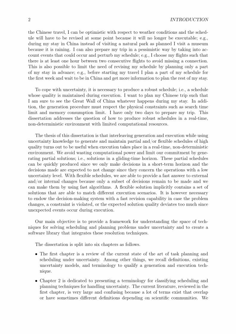
Figure 1.1 shows a toy example of a classic planning problem in the blocks world; onthe left-hand side is the initial state and on the right-hand side is the goal state. In theinitial state, the two blocks are placed on a table (C and B) and block A is piled up onblock B; we have to move them one after the other in such a way as to reach the goal state(A on the table, C on A, and B on C). We assume there is only one hand to move blocksand this hand can only hold one block at a time. In addition, there are some rules, calledpreconditions, that have to be verified to change the current world state; e.g., we cannotmove a block X on Y if there is another block piled up on X or on Y . The operator inthis planning problem can be expressed as follows in the STRIPS language [65]:Move(?X, ?Z, ?Y):Preconditions: Free(?Y), Free(?X), On(?X, ?Z)Effects: On(?X, ?Y), ¬ Free(?Y), Free(?Z)Operator Move requires three parameters: ?X represents the block we want to move, ?Yrepresents the block/table on which we want to place ?X, and ?Z represents the block/tableon which ?X is placed before moving it.
A solution of a planning problem is a plan; i.e., a solution is a set of actions that arepartially or fully ordered. In other words, we have to find a path through the state spaceto go from the initial state to the goal state. A solution of the blocks world problem aboveis a set of three totally ordered actions: place A on the table, pile up C on A, and pileup B on C. In the STRIPS language, the solution is expressed as follows: Move(A, B,table), Move(C, table, A), Move(B, table, C).
Classical task planning assumes there is no uncertainty; e.g., the effects of actions areknown. This implies that outputs and inputs of the execution system are independent,this is called an open-loop execution.
1Task planning is different from production planning since operations to execute are known in pro-duction planning and production planning focuses on the question of when to produce goods and whatresources to use given production orders and due dates.
1.2. DETERMINISTIC DOMAINS 7
Free(A)
Free(C)
¬Free(B)
On(A, B)
Free(B)
¬Free(C)
¬Free(A)
On(B, C)
On(C, A)
A
B C
B
C
A
Figure 1.1: A toy example of a task-planning problem.
1.2.2 Scheduling
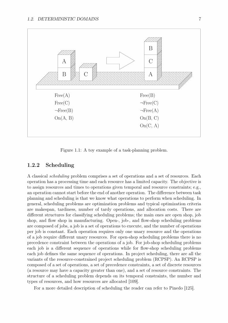
A classical scheduling problem comprises a set of operations and a set of resources. Eachoperation has a processing time and each resource has a limited capacity. The objective isto assign resources and times to operations given temporal and resource constraints; e.g.,an operation cannot start before the end of another operation. The difference between taskplanning and scheduling is that we know what operations to perform when scheduling. Ingeneral, scheduling problems are optimization problems and typical optimization criteriaare makespan, tardiness, number of tardy operations, and allocation costs. There aredifferent structures for classifying scheduling problems; the main ones are open shop, jobshop, and flow shop in manufacturing. Open-, job-, and flow-shop scheduling problemsare composed of jobs, a job is a set of operations to execute, and the number of operationsper job is constant. Each operation requires only one unary resource and the operationsof a job require different unary resources. For open-shop scheduling problems there is noprecedence constraint between the operations of a job. For job-shop scheduling problemseach job is a different sequence of operations while for flow-shop scheduling problemseach job defines the same sequence of operations. In project scheduling, there are all thevariants of the resource-constrained project scheduling problem (RCPSP). An RCPSP iscomposed of a set of operations, a set of precedence constraints, a set of discrete resources(a resource may have a capacity greater than one), and a set of resource constraints. Thestructure of a scheduling problem depends on its temporal constraints, the number andtypes of resources, and how resources are allocated [109].
For a more detailed description of scheduling the reader can refer to Pinedo [125].

8 CHAPTER 1. STATE OF THE ART
Figure 1.2 represents a small job-shop scheduling problem with three jobs. Operationsare not preemptive; i.e., they cannot be interrupted once they have started to execute.Allocations have already been done and each resource; e.g., a workshop machine, canonly perform one operation at a time. We assume we want to minimize the makespanof the solution, where the makespan is the duration between the start time of the firstoperation and the end time of the last operation of the schedule. The optimal solution ofthis problem is represented on Figure 1.3.
Resource 3Duration 28
Resource 3Duration 54
Resource 3Duration 26
Resource 1Duration 33
Resource 1Duration 68
Duration 52Resource 1
Resource 2Duration 46
Res. 2Dur. 20
Resource 2Duration 26
Job 3
Job 2
Job 1
Figure 1.2: A toy example of a job-shop scheduling problem.
makespan 179
Resource 1Duration 33 Duration 68
Resource 1Duration 52Resource 1
Res. 2Dur. 20
Resource 2Duration 46
Resource 3Duration 28 Duration 26
Resource 3Duration 54Resource 3
Resource 2Duration 26
Figure 1.3: A toy example of an optimal job-shop scheduling solution.
1.2.3 Bridging the Gap Between Task Planning and Scheduling
Many real-life problems involve both task planning and scheduling because they containresource requirements, as well as causal and temporal relationships. In this sense, aclassical planning problem is a relaxed real-world problem because it does not take intoaccount resources and time. A scheduling problem is an overconstrained real-life problem

1.2. DETERMINISTIC DOMAINS 9
because all operations are known before scheduling and we cannot change them; no causalreasoning is done and scheduling can be seen as a sub-part of task planning that is usuallynot taken into account by task planning. Task planning and scheduling are complementarybecause each of them considers different aspects of a real-life combinatorial problem.
Smith, Frank, and Jónsson demonstrated how many difficult practical problems liesomewhere between task planning and scheduling, and that neither area has the right setof tools for solving these problems [149].
Temporal planning permits one to represent time explicitly and to take a step towardsscheduling. Actions have start and end times and there are delays between actions. Aneffect may begin at any time before or after the end of an action. Events occurring atknown times can be taken into account.
Planning with resources is being developed and allows to bridge the gap between plan-ning and scheduling by taking into account resource requirements [96, 92]. Laborie workedon integrating both plan generation and resource management in a planning system [95].At NASA Ames, a system that is based on a framework aiming at unifying planning andscheduling was developed [114].
Some researchers are working on extended scheduling problems by considering thereare alternative process plans for example. A process plan is a subset of operations thatare totally ordered. A subset of operations to schedule have to be chosen [90, 19].
Both classical task planning and scheduling are limited because they assume the en-vironment is deterministic. In task planning, actions are deterministic; i.e., we knowthe effects that are produced when actions are performed. In scheduling, operation du-rations are precisely known and resources do not break down. Section 1.3 focuses onnon-deterministic task planning and scheduling.
1.2.4 Models
In this section, we present some models that are used to represent static task planningand scheduling problems when execution is assumed to be deterministic. Each model isassociated with a set of search algorithms to solve instances of these problems.
Constraint-Satisfaction Problem
A classical Constraint-Satisfaction Problem is a tuple 〈V, D, C〉, where V is a finite setof variables, D is the set of corresponding domains, and C = c1, . . . , cm is a finite set ofconstraints. A constraint is a logical and/or mathematical relationship in which at leastone variable is expressed. A solution is a complete consistent value assignment that issuch that the assignment of values for the variables in V satisfies all the constraints inC. For rigorous definitions of the basic concepts, we refer the reader to Dechter [48] andTsang [159].
Although its definition does not require it, the CSP as defined above is classicallyformulated for variables with discrete domains, typically a finite set of symbols or aninteger interval. The CSP has also been formulated for variables with continuous domains,typically a real interval [104], when it is called a numerical CSP.
Propagation algorithms , also called filtering algorithms, are used to remove values fromvariable domains and determine if the CSP is not consistent; i.e., a CSP is not consistentif a variable domain becomes empty after propagation. There can be different algorithms

10 CHAPTER 1. STATE OF THE ART
with different complexities and different inference powers for a given constraint; e.g., thealldiff constraint can be implemented in different ways [131]. Propagation is initiallydone before starting search and then it might be incrementally done during search; i.e.,whenever a variable domain is changed, a propagation is done to update variable domainswith respect to constraints.
A scheduling problem can be represented by a constraint network such that operationstart times, operation durations, operation end times, resource capacities, and optimiza-tion criteria are variables. There are particular propagation algorithms such as temporalpropagation for temporal constraints, timetables [100], edge-finder [119, 18], the balanceconstraint for resource capacity constraints [96], etc.
A temporal task-planning problem can also be represented by a constraint network.Constraint-Based Interval (CBI) planning makes use of an underlying constraint networkto keep track of the actions and the constraints in a plan [64]. For each interval in the plan,two variables are introduced into the constraint network, corresponding to the beginningand ending points of the interval. Constraints on the intervals then translate into simpleequality and inequality constraints between end points. Interval durations translate intoconstraints in the distances between start and end points. Inference and consistencychecking in the temporal network can often be accomplished using fast variations of arc-consistency, such as Simple Temporal Propagation [51]. Vidal and Geffner have recentlyproposed constraint propagation rules for solving canonical task-planning problems [168].Canonical task planning is halfway between full temporal task planning and scheduling:while in scheduling, typically every action (operation) is done exactly once, in canonicaltask planning, it is done at most once, in full temporal task planning, it may be done anarbitrary number of times.
Laborie has developed filtering algorithms for making search of minimal critical setsmore efficient when planning or scheduling with resources [95, 97].
Mathematical Programming
Mathematical Programming is an alternative to CSP to model and solve optimizationproblems when all constraints can be expressed by linear relationships. There are mainlytwo ways of modeling such a problem: Mixed Integer Program (MIP) or Linear Pro-gram (LP). In a MIP some variables are integers whereas there are only real variables inan LP. In general, there are more variables in a mathematical program than in a CSPbut their domains are smaller. An LP is solved by the simplex method. The simplexmethod is very easy to use and can find optimal solutions. Branch-and-cut can efficientlysolve a MIP whose continuous relaxation is a good approximation of the convex hull ofinteger solutions and/or around the optimal solution, or for which this relaxation canbe reinforced by adding cuts. The continuous relaxation consists in removing integralityconstraints and cuts are linear relationships. Lagrange multipliers, duality, and convexitycan also be used to solve these programs. Compared to the CSP approach it is less easyto formalize a mathematical program and obtain a model that can be efficiently solvedwithout exponentially increasing the number of integer variables or the number of con-straints. In addition, even if some non-linear expressions can be linearized, for examplethe disjunctions, or the logical constraints more generally, their formulations often resultin weak linear relaxations and thus in an inefficient solving. Queyranne and Schulz pro-pose a review of some mixed integer programs with a polyhedral study [130]. For a recent

1.3. NON-DETERMINISTIC DOMAINS 11
state-of-the-art review in integer programming the reader can refer to Wolsey [178].Several planners have been constructed that attempt to check the consistency of sets
of metric constraints even before all variables are known. In general, this can involvearbitrarily difficult mathematical reasoning, so these systems typically limit their analysisto the subset of metric constraints consisting of linear equalities and inequalities. Severalrecent planners have used LP techniques to manage these constraints [123, 124, 157, 177].
The operations research community has been interested in solving scheduling problemsby using MIP since its beginnings. In particular, some works have been done on theResource-Constrained Project Scheduling Problem [11, 17, 66, 121, 156, 154]. In thisproblem, resource constraints are hard to model with linear inequalities because it isnecessary to keep track of the set of operations during execution at any time. Mostresearchers who use MIP for modeling RCPSPs work around this problem by discretizingtime, but many additional variables have to be used depending on time horizon.
1.2.5 Optimization
The solutions are not equal in every combinatorial problem. In scheduling, for instance,the user might deem schedules with shorter makespans to be preferable to those withlonger makespans. Indeed, optimization is a discrimination between solutions by nature.
In a constraint optimization problem (COP), solutions are ordered partially or totallyaccording to optimization criteria [108]. An optimization criterion is an arithmetic ex-pression over a subset of variables of the problem; e.g., tardiness depends directly on whenoperations finish with respect to due dates but is not directly dependent on what resourcesare used. Without loss of generality, solutions are sought that satisfy all constraints andminimize an objective function; e.g., we want to find a schedule that does not violateprecedence and resource constraints and minimizes makespan. When using a constraint-based approach branch-and-bound can be applied to make search more efficient; e.g., afirst solution is found heuristically and gives a first value of the objective function, thenthe problem is incrementally strengthened by posting an additional constraint bound bythe best optimization value.
When using a linear program to model an optimization problem with linear constraints,the simplex or interior point methods can be used to find the optimal solution if one exists.
1.3 Non-deterministic Domains
In this section, we review the literature about task planning and scheduling when weassume solutions are executed in a non-deterministic environment because unexpectedevents occur during execution; e.g., new goals to attain and/or new operations to perform.In some cases, we do not know precisely when some expected events occur; e.g., resourcebreakdown end times. In other words, the environment is imprecisely and/or partiallyknown and its evolution is described by distributions.
1.3.1 Uncertainty Sources
Uncertainty is a general term but we can distinguish uncertainty from imprecision. Anuncertain event means that we do not know if this event will occur or not whereas an

12 CHAPTER 1. STATE OF THE ART
imprecise event means that we do not exactly know when this event is going to occurbut we know for sure it is going to occur. A risk can be associated with the occurrenceof an event and means the occurrence of the event impacts the solution quality. Giventhe occurrence of an event we are given a set of decisions to make. Each decision has aconsequence. Decision theory is a research domain in which the desirability of a decisionis quantified by associating a utility (or desirability) measure with each outcome. In therest of this dissertation we shall not be concerned with risk.
In this section, we list a number of uncertainty sources in task planning and schedulingwithout being exhaustive.
In task planning, we may have to address the following problems:
• some actions have imprecise effects; e.g., after having moved, the position of a robotis not precisely known;
• world states are partially observable or not observable; e.g., the position of the robotis unknown because it is not equipped with sensors;
• world states are uncertain independently of actions and need information gathering;e.g., a robot can reach an area by taking one of two alternative paths depending onground composition, that is to say, the robot has to analyze a ground sample beforemoving;
• new subgoals are added during execution.
In scheduling, we may have to deal with the following problems:
• some operation processing times/durations or some earliest operation start timesare not precisely known a priori ;
• some resource capacities or states are imprecise a priori ; e.g., the mean time betweenfailures of a resource can be used, we do not the exact start time of a breakdown;
• some resource quantities required by some operations are imprecise and/or uncertain(no resource may be required) a priori ; e.g., we do not know precisely how manyworkers are needed to lay the foundations of a dam because of uncertain/partialknowledge of the geological conditions before starting to work;
• uncertain and/or imprecise production orders;
• new operations to be scheduled and executed may only be known during execution;e.g., we have to inject some cement into the foundations because we observe theyare not enough strong via specific sensors.
1.3.2 Definitions
In this section, we give some general definitions for a better understanding of the literature.The first three definitions explain some characteristics of a problem to solve such thatits solution will be executed. The problem is composed of variables, such as operationdurations, operation start times, or the state of a resource.

1.3. NON-DETERMINISTIC DOMAINS 13
Definition 1.3.1 (effectiveness). An effective plan/schedule is a plan/schedule obtainedafter execution. An effective plan/schedule is fully set; i.e., all variables have been instan-tiated.
After a variable is effectively instantiated, we can no longer change it.
Definition 1.3.2 (event). An event is a piece of information about the world state.
For example, the end time of an operation with an imprecise processing time is anevent since we do not know precisely when this operation ends before observing it isfinished. In other words, we do not know its effective end time date before it occurs.
A dynamic problem is a problem that changes during execution, whereas a staticproblem does not change during execution. For example a scheduling problem is dynamicbecause operations are added or removed during execution, distributions associated withits random variables are changed during execution, etc. Notice that a static problem canbe defined by imprecise data.
For example a scheduling problem with breakable resources can be considered as adynamic problem if the exact number of resource breakdowns is not known before execu-tion. However, a scheduling problem with imprecise processing times is a static problemsince we know the set of events in advance; i.e., we know the set of operation start andend times in advance.
A deterministic problem is a static problem by nature since all events are known inadvance but a non-deterministic problem; i.e., a problem with random variables can beeither static or dynamic.
The following definitions concern the generation process that is the procedure used tofind a solution of a problem.
Definition 1.3.3 (predictive decision-making process). Predictive planning/schedulingconsists in making all decisions before execution starts.
In the literature, some authors use the term baseline schedule instead of predictiveschedule.
Definition 1.3.4 (reactive decision-making process). Reactive planning/scheduling con-sists in making all decisions as late as possible; i.e., decisions are taken and executedwithout anticipation during execution.
Predictive and reactive planning/scheduling are two extremes because in the formerall decisions are made before execution with anticipation and in the latter no decision ismade in advance.
Definition 1.3.5 (off-line reasoning). Off-line reasoning consists in taking decisions be-fore execution starts.
When reasoning off line a predictive schedule/plan is typically generated off line andpassed on to the execution manager. This reasoning is usually static; i.e., the predictiveschedule/plan is completely generated and all decisions are taken at the same time. Sucha reasoning is deliberative; i.e., we take decisions in advance of their executions and wehave time to reason.

14 CHAPTER 1. STATE OF THE ART
Definition 1.3.6 (on-line reasoning). On-line reasoning is concurrent with the physicalprocess execution.
On-line reasoning is dynamic by nature because the generation of a schedule/planis incremental ; i.e., the schedule/plan is completed as long as execution goes on. Thisreasoning usually needs to meet real-time requirements ; i.e., decisions have to be madegiven a time limit. Such a reasoning can be deliberative and/or reactive to events. It isalso possible to change decisions during execution.
Table 1.1 summarizes the characteristics of the generation and execution processesunder uncertainty and/or change.
When a solution is executed, some elements of its execution environment may change;e.g., the state of a resource changes. In general, there are real-time requirements whenexecuting a solution; i.e., if some basic decisions have still to be made the time for com-putation is limited; e.g., operation start times have to be quickly decided. Executiondecisions are decisions to adapt the flexible solution with respect to what happens duringexecution. The decision-making system might be able to react in response to occurringevents; i.e., it can make execution decisions when some events occur. For example, whenthe state of a resource changes, we may have to decide what alternative operations toexecute.
The generation of a solution can be made off and/or on line. When a solution is gen-erated off line we usually have time to make decisions whereas we have a limited time formaking decisions during execution due to the dynamics of the underlying physical systemand its execution environment. Generation decisions are decisions made to anticipatewhat is going to happen during execution. Sometimes the system must be able to changedecisions on line when the solution is no longer executable; e.g., a resource breaks downand we have to reallocate some operations that have to be executed in the near future.
Execution GenerationProcess: solution Off-line On-linebeing executed scheduling/ scheduling/
on line planning planningDynamic=changes Yes Usually not Yesover time: states. . .
Real time=time- Yes, but only No Yesbounded computation basic decision-makingReactive=in response Might be No Might be
to events
Table 1.1: Off-line/On-line reasoning.
In the ideal world, there is no unexpected event that can occur and affect the sched-ule/plan quality or make the schedule/plan unexecutable during execution, so the pre-dictive plan/schedule is generated off line and then executed. Figure 1.4 represents thegeneration-execution loop in the ideal world. A plan/schedule is generated off line andsent to the execution controller. The latter drives the underlying physical system by send-ing orders (actions) to actuators. The sensors of the physical system send information(events) to the execution controller that updates the plan/schedule accordingly; i.e., itindicates what events have been executed and updates clock. The execution controller

1.3. NON-DETERMINISTIC DOMAINS 15
plays the role of an interface between the solution generator and the physical system.Note however that in the case of the ideal world we do not need to observe events sincethere is no unexpected event and the occurrences of events are precisely known.
Planning/Scheduling
Plan/Schedule
off line
on line
real world
Actions
Events
solution execution
update
Execution controlling
Figure 1.4: Generation and execution in the ideal world.
However, the predictive schedule/plan will not always fit the situation at hand becausethere are uncertainty and change; i.e., data is imprecise and/or uncertain. In such asituation, we have to decide what to do to cope with uncertainty and change: we couldadapt the schedule/plan on line, we could make the initial schedule/plan less sensitiveto execution environment, and/or we could find a compromise between both options;Sections 1.3.5 and 1.3.6 present some techniques to handle uncertainty and change. Thenext section is dedicated to reviewing uncertainty sources in task planning and scheduling.
1.3.3 Uncertainty Models
A number of different models have been proposed and used to represent uncertainty inscheduling and task planning. In this section, we present these uncertainty models andgive their main properties. Moreover, we discuss Bayesian approach since it is a promisingway for dealing with uncertainty in scheduling and planning.

16 CHAPTER 1. STATE OF THE ART
Probability Theory
The probability theory is based on the notion of sets; it uses unions and intersections of sets.In the probability theory a random variable X can be instantiated to value v belongingto a discrete or continuous domain D; i.e., it is a probability distribution Pr(X = v).
The formal definition is the following: ∀v ∈ D, 0 ≤ Pr(X = v) ≤ 1 and if we com-pletely know the probability distribution:
∑v∈D Pr(X = v) = 1.
It is possible to express dependence between variables. A conditional probability suchas the occurrence of event A knowing the occurrence of event B is expressed as follows:
Pr(A|B) =Pr(A, B)
Pr(B),
where Pr(A, B) is the probability that both A and B occur at the same time and is calledthe joint probability. This is then possible to compute the marginal probability of A:Pr(A) =
∑v∈D(Pr(A|X = v) × Pr(X = v)). If A and B are independent events then:
Pr(A, B) = Pr(A)× Pr(B).Probabilities can be used to model imprecise operation processing times [21] or action
effects in task planning [32] but they require statistical data that do not systematicallyexist. In addition, probabilities are easy to interpret but cannot represent full or partialignorance.
Bayesian Networks Bayesian networks are acyclic directed graphs [122]. Each nodeis associated with a finite domain variable, each variable domain is associated with aprobability distribution, and each arc represents a causal relation between two variables.Each pair of dependent variables is associated with a table of conditional probabilities.For example if the duration of an operation depends on the outside temperature andhumidity this yields the Bayesian network of Figure 1.5a, where Figure 1.5b depicts thelink matrix necessary for full characterization of the causal relation. According to thismatrix we know that the probability that the operation duration is 15 minutes if theoutside humidity is less than 40 per cent and the outside temperature is less than 20
Celsius equals 0.1.A Bayesian network contains the information needed to answer all probabilistic queries.
A Bayesian network can be used for induction, deduction, or abduction. Induction con-sists in determining rules by learning from cases, just like neural nets. Deduction is alogic procedure in which we reason with rules and input facts to determine output facts.Abduction is a way of reasoning such that output facts are symptoms that are observedwhereas decisions must be taken as which input facts produced the observed symptoms.
A Bayesian network is a static representation (no anteriority); it can not representtime but is able to model incomplete knowledge.
Bayesian networks have some limitations. Inference in a multi-connected Bayesian net-work is NP-hard. Variables are discrete, and the number of arcs is limited for performancereasons. In addition, Bayesian inference can only be done with a complete probabilisticmodel. However, when dealing with discrete probability distributions associated withsome input facts it is possible to compute approximate probability distributions of outputfacts by using Monte-Carlo simulation. The only issue when generating a realization is topick up first the random values of the independent variables. Bayesian networks have the

1.3. NON-DETERMINISTIC DOMAINS 17
(b)
outsidetemperature
outside
duration
operation
humidity
(a)
outside humidity
outside temperature
< 40%
< 20 Celsius
between 40% and 60%
< 20 Celsius
> 60%
< 20 Celsius
< 40%
between 40% and 60%
between 20 and 30 Celsius
between 20 and 30 Celsius
< 40%
> 30 Celsius
between 40% and 60%
> 30 Celsius
> 60%
> 60%
> 30 Celsius
duration
operation
between 20 and 30 Celsius
0.75
0.15
0.05
25 minutes15 minutes
0.9
0.2
0.3
0.8
0.6
0.85
0.65
0.1
0.7
0.4
0.35
0.25
0.95
0.45 0.55
Figure 1.5: (a) A Bayesian network and (b) a conditional probability matrix characterizingthe causal relation.
same advantages and drawbacks as probabilities: it requires statistical data and cannotrepresent ignorance.
Recently some work has been done to combine CSPs with Bayesian Networks [128].
Influence diagrams [86] extend Bayesian networks by adding random utility variablesand non random decision variables to the usual random variables. A non random decisionvariable is instantiated by a decision-maker, and random utility variables are used torepresent the objective (or utility) to be maximized.
Dynamic Bayesian Networks [47] (DBNs) are another extension to Bayesian networksthat can model dynamic stochastic processes. A DBN can model changes in a world stateover time. DBNs fail to model quantitative temporal constraints between actions in acomputationally tractable way and suffer from the problem of unwarranted probabilitydrift; i.e., probabilities associated with facts depend upon how many changes in the worldstate have occurred since the last time probabilities were computed.
Hybrid or mixed networks [49, 50] allow the deterministic part of a Bayesian networkto be represented and manipulated more efficiently as constraints.

18 CHAPTER 1. STATE OF THE ART
Theory of Fuzzy Sets and Possibility Theory
Zadeh has introduced the theory of fuzzy sets that is based on the generalization of thenotion of set [181].
The characteristic function of a subset A of a universal set Ω associates the value 1 toany element of Ω if this element is in A and the value 0 if this element is not in A. Onthe contrary, for a fuzzy subset it is possible to define intermediate membership degreesbetween these two extremes.
More formally, a fuzzy subset is defined as follows. A fuzzy subset A of a universal setΩ is defined by a membership function µ : Ω → [0, 1]. For any element ω in Ω the valueµA(ω) is interpreted as the membership degree of ω to A.
The possibility theory is a convenient means to express uncertainty [182]. With thistheory it is possible to explicitly take into account uncertainty associated with the occur-rences of events. In such a model uncertainty associated with an event e is described by apossibility degree that e occurs and a possibility degree that the opposite event e occurs.
In general, a possibility distribution over a universal set Ω (the set of possible events)is a function π : Ω → [0, 1] defined such that there exists at least one ω ∈ Ω such thatπ(ω) = 1.
From a possibility distribution over Ω it is possible to define a possibility measure Πand a necessity measure N of a part A of Ω as follows:
Π(A) = supω∈A
π(ω) and N(A) = infω∈CA
Ω
(1− π(ω)),
where CAΩ is the complementary part of A in Ω. Notice that for any part A of Ω, the
possibility measure and the necessity measure are related by the following formulas:
N(A) = 1− Π(CAΩ ) and Π(A) ≥ N(A).
In practice, different interpretations of these functions π can be made.
• It is possible to represent an occurrence possibility with π(X = v); i.e., the possi-bility that variable X is instantiated with value v.
• We can express similarity with π(E is cpt) that represents the degree to whichelement E is similar to concept cpt (represented by a function); e.g., Figure 1.6represents a similarity function with respect to the concept “young.”
• It is also possible to express preferences with π(X = v) that represents the satisfac-tion degree when variable X is equal to value v.
With a possibility function, it is possible to represent both imprecision and uncer-tainty. For example we can represent the fact that we do not know precisely and withtotal certainty how many workpieces are produced in a workshop; we can only expressa possible and imprecise number between 200 and 400, the possible fact that no work-piece are produced at all, and it is not fully possible but we may produce 600 workpieces;Figure 1.7 represents such a possibility function. Such a function can also represent thefuzzy processing time of an operation for example, see Section 1.3.6.
The classical concept of set is limited for representing vague knowledge, and probabilitytheory is not able to represent subjective uncertainty and ignorance, however, fuzzy logicand the theory of possibility overcome these difficulties. The main drawback of the fuzzyrepresentation is the subjective way for interpreting results.

1.3. NON-DETERMINISTIC DOMAINS 19
0 10 20 30 40 50 60 70 80 90 100Age (years)
0
0.2
0.4
0.6
0.8
1
Figure 1.6: A possibility function of the concept “young.”
0 100 200 300 400 500 600 700Number of produced workpieces
0
0.5
1
Figure 1.7: A possibility function for a number of produced workpieces.

20 CHAPTER 1. STATE OF THE ART
robot inroom 4
robot inroom 3
robot inroom 7
R(room7) = 6
R(room5) = 5R(room6) = −1
robot inroom 6
R(room3) = −4
R(room4) = 3
T (room4, moveright, t1) = 0.7
robot inroom 5
T (room5, moveforward, t1) = 0.4
T (room4, moveforward, t1) = 0.8
T (room4, moveforward, t1) = 0.2
T (room3, moveright, t1) = 0.7
T (room4, moveright, t1) = 0.3
T (room6, moveleft, t1) = 0.9 T (room5, moveforward, t1) = 0.6
T (room6, moveleft, t1) = 0.1
Figure 1.8: An illustrative example of the graphical view of an MDP.
Markov Decision Processes
A Markov Decision Process can be seen as a timed automaton such that each transitionfrom one state to another state is associated with a probability of being fired. Moreformally an MDP can be defined as follows: an MDP has four components, S, A, R, T . S(|S| = n) is a (finite) state set. A (|A| = m) is a (finite) action set. T (s, a, t) is a transitionfunction that depends on time t, and each T (s, a,−) is a probability distribution over Srepresented by a set of n× n stochastic matrices.2 R(s) is a bounded, real-valued rewardfunction represented by an n-vector. R(s) can be generalized to include action costs:R(s, a). R(s) can be stochastic (but replaceable by expectation).
MDPs can model transition and/or stochastic systems; i.e., it is possible to model howa process evolves during execution (the state of a system can change over time dependingon what actions are performed) [70, 129]. MDPs are related to decision-theoretic plan-ning [33] and used to model state-spaces in the task-planning context. General objectivefunctions (rewards) can be expressed. Policies are general solution concepts that consistin choosing what action to perform in each visited state to maximize the total reward.MDPs provide a nice conceptual model: classical representations and solution methods
2Note that Sabbadin [135] proposed to use possibilistic MDPs.

1.3. NON-DETERMINISTIC DOMAINS 21
tend to rely on state-space enumeration whereas MDPs are able to easily represent thisspace. Figure 1.8 is a graphical view of MDP that represents the state space of a smalltask-planning problem in which a robot must go from room 3 to room 7. There are threeoperators: move right, move left, and move forward. This MDP is valid at time t1 whenthe robot is in room 4. In the current state, only one of two actions can be performed:move either right or forward. If action moveforward is activated, the probability that therobot does not move is equal to 0.2 and the probability that it actually goes from room4 to room 6 equals 0.8. Each state s represents the possible position of the robot; i.e., sindicates the room it is in. The probabilities that are not represented equal zero.
MDP is a model easily generalizable to countable or continuous state and action spaces.The main drawback of MDP is the need to enumerate and represent all possible states;i.e., it is time and memory consuming.
Partially Observable MDPs [106] take into account the fact that each state of thedynamic process is generally indirectly observable via potentially erroneous observations.In task planning, an observation consists in general in performing an action to gather newinformation.
Dynamic programming [23, 24] is used to solve MDPs. The main issue of MDPs isthe number of states to develop; so some work has been done for finding a more compactrepresentation; for example, Factored MDPs [34] extend MDP concepts and methods toa variable-based representation of states and decisions.
Sensitivity Analysis
Sensitivity analysis consists in defining how much we can perturb a problem withoutdegrading the quality of the solution of the initial problem. In other words, sensitivityanalysis, combined with parametric optimization, is a way of checking if the solution ofa deterministic linear program is reliable, even if some of the parameters are not fullyknown but are instead replaced by estimated values. When doing a sensitivity analysis,we are interested in knowing the robustness of a solution; i.e., to what extent this solutionis insensitive to changes of the initial problem with respect to its quality, in particular,what are the limits to a parameter change (or several changes) such that the solutionremains optimal? However, sensitivity analysis has some limitations since it is based ondeterministic models and is thus useful only as far as variation of controllable parametersis concerned [171].
Application of sensitivity analysis has been done in scheduling [78, 153].
Stochastic Programming
Stochastic programming [29] is a mathematical programming paradigm, see Section 1.2.4,which explicitly incorporates uncertainty in the form of probability distributions of someparameters. There are decision variables and observations; i.e., observations are values ofthe random parameters. In a recourse problem, decisions alternate with observations in anm-stage process; i.e., at each stage, decisions are made, and observations are done betweenstages; there are initial decisions made before any observation and recourse decisionsmade after observations. The number of stages gives a so-called finite horizon to theprocess. A decision made in stage s should take into account all future realizations ofthe random parameters and such decision only affects the remaining decisions in stagess+1, s+2 . . . m. In Stochastic Programming, this concept is known as non-anticipativity.

22 CHAPTER 1. STATE OF THE ART
The convex optimization function depends on decisions and observations. The goal is tooptimize the expected value of the optimization function such that random parameters arenot necessarily independent of each other; they are however independent of decisions. Oneapproach to solving this problem is to use an expected value model that is constructedby replacing the random parameters by their expected values. Another solving processconsists in generating n scenarios such that each scenario; i.e., any possible set of values forthe parameters represents a deterministic mathematical program that is then solved [55].Once the n programs have been solved, decisions that are common to the most solutionsare made for solving the stochastic program. One of the issues of this approach is thenumber of scenarios that are necessary to solve the problem and the related efficiencyissue.
Extensions of the Constraint-Satisfaction Problem
We review the main constraint-satisfaction problem frameworks that can deal with un-certainty and change. For a more detailed review, the reader can refer to the recentpaper of Verfaillie and Jussien [162]. These frameworks are extensions of the Constraint-Satisfaction Problem framework presented in Section 1.2.4.
Dynamic CSP A Dynamic Constraint-Satisfaction Problem (DCSP) consists in a se-ries of CSPs that change permanently or intermittently over time, by loss or gain of values,variables or constraints. The objective is to find stable solutions to these problems; i.e.,solutions that remain valid when changes occur. Wallace and Freuder tackled these prob-lems [169]. The basic strategy they use is to track changes (value losses or constraintadditions) in a problem and incorporate this information to guide search to stable solu-tions. The objective for them is to find a trade-off between solution stability and searchefficiency. A probabilistic approach is used: each constraint C is associated with a valuethat gives the probability that C is part of the problem. Probabilities of change are notknown a priori.
Elkhyari et al. study scheduling problems that change during execution and use DCSPsto model and solve them [56]. In particular, they study Resource-Constrained ProjectScheduling Problems. They use explanations by determining conflict sets, also known asnogoods, to solve these problems.
Conditional CSP The Conditional Constraint-Satisfaction Problem [137] framework(CCSP) was first named Dynamic Constraint-Satisfaction Problem [111]. CCSPs havebeen studied by a number of researchers [35, 136, 152, 71, 138]. The basic objective of theCCSP framework is to model problems whose solutions do not all have the same structure;i.e., do not all involve the same set of variables and constraints. Such a situation occurswhen dealing with product configuration or design problems, because the physical systemsthat can meet a set of user requirements do not all involve the same components. Moregenerally, it occurs when dealing with any synthesis problem, such as design, configuration,task planning, scheduling with alternatives, etc. In a CCSP, the set of variables is dividedinto two parts: a subset of mandatory variables and a subset of optional ones. The setof constraints is also divided into two parts: a subset of compatibility constraints and asubset of activity constraints. Compatibility constraints are classical constraints. Activityconstraints define the conditions of activation of the optional variables as functions of the

1.3. NON-DETERMINISTIC DOMAINS 23
current assignment of other mandatory or optional variables. Constraints are activated iftheir respective variables are activated too. When solving a CCSP its structure (activatedvariables and constraints) may change because it depends on the current assignment.Thus, a CCSP can be considered as a particular case of DCSP where all the possiblechanges are defined by the activity constraints.
Open CSP The Open Constraint-Satisfaction Problem [60] framework (OCSP) wasfirst named Interactive Satisfaction Problem [98]. In an OCSP, the allowed values indomains, as well as the allowed tuples in relations, may not be all known when startingsearch for a solution. They may be acquired on line when no solution has been foundwith the currently known values and tuples. Such a situation occurs when the acquisitionof information about domains and relations is a costly process that needs either heavycomputation or requests to distant sites. An OCSP can thus be considered as a particularcase of DCSP where all the possible changes result in extensions of the domains andrelations.
Mixed CSP The Mixed Constraint-Satisfaction Problem [63] framework (MCSP) mod-els decision problems under uncertainty about the actual state of the real world. In anMCSP, variables are either controllable (decision variables) or uncontrollable (state vari-ables). Decision variables are under the control of the decision agent whereas state vari-ables are not under its control. In this framework, a basic request may be to build adecision (an assignment of the decision variables) that is consistent whatever the state ofthe world (the assignment of the state variables) is. An MCSP can not model problemchanges but imprecision, therefore MCSP and DCSP are complementary.
Probabilistic CSP The Probabilistic Constraint-Satisfaction Problem framework (PCSP)models decision problems under uncertainty about the presence of constraints [61]. In aPCSP, a probability of presence in the real world is associated with each constraint. Insuch a framework, a basic request may be to produce an assignment that maximizes itsprobability of consistency in the real world. A PCSP is a particular case of the ValuedConstraint-Satisfaction Problem framework (VCSP) [144, 30].
Fuzzy CSP The Fuzzy Constraint-Satisfaction Problem framework (FCSP) models de-cision problems where possibility distributions are associated with variable domains [134].In such a framework, we are interested in finding a solution that satisfies constraints andmaximizes the satisfaction degree whatever the effective instantiations of variables turnout to be. The satisfaction degree of a solution is the combination of the possibility degreescorresponding to the assigned values. This framework is subsumed by the semiring-basedCSP framework [30].
Stochastic CSP The Stochastic Constraint-Satisfaction Problem [172] framework (SCSP)models decision problems under uncertainty about the actual state of the real world, thesame way as the MCSP framework. The SCSP framework is inspired by the Stochas-tic Satisfiability Problem framework (SSAT) [105]. As in an MCSP, variables are, inan SCSP, either controllable (decision variables) or uncontrollable (state variables). The

24 CHAPTER 1. STATE OF THE ART
main difference between an MCSP and an SCSP is that decision variables have not neces-sarily to be instantiated before state variables in an SCSP. In such a framework, a basicrequest may be, as in a PCSP, to build a decision (an assignment of the decision vari-ables) that maximizes its probability of consistency in the real world. A recent proposal,the Scenario-based Constraint-Satisfaction Problem [107] framework, is an extension ofSCSP along a number of dimensions: multiple chance constraints and new objectives. Itis inspired by Stochastic Programming, see Section 1.3.3. In this framework, there are twokinds of constraints: hard constraints that must always be satisfied and chance constraintswhich may only be satisfied in some of the possible worlds. Each chance constraint hasa threshold, θ and the constraint must be satisfied in at least a fraction θ of the worlds.Stochastic constraint programs are closely related to MDPs 1.3.3. Stochastic constraintprograms can, however, model problems which lack the Markov property that the nextstate and reward depend only on the previous state and action taken. The current de-cision in a stochastic constraint program will often depend on all earlier decisions. Tomodel this as an MDP, we would need an exponential number of states.
1.3.4 Temporal Extensions of CSPs
In this section, we describe some extensions of the CSP framework that can deal withtime. Therefore, these frameworks are particularly suited to temporal task planning,scheduling, and other temporal application domains.
Temporal Conditional CSPs
Conditional CSPs have been adapted to temporal problems to be able to represent alter-natives. An alternative is a subset of temporal constraints. By nature, each alternativebelongs to a set whose elements are mutually exclusive. Tsamardinos, Vidal, and Pol-lack [158] have proposed a new constraint-based formalism with temporal constraints.In this paper, they present a procedure that is able to check whether such a constraintnetwork is consistent whatever alternatives are chosen.
Temporal CSPs with Uncertainty
The Temporal CSP with Uncertainty framework is directly inspired by MCSPs and ap-plied in the temporal context. A usual strategy to deal with uncertainty, referred to asleast commitment strategy, consists in deciding about some crucial choices (for examplethe selection and sequencing of operations) and letting another process (for example exe-cution control) make the remaining decisions (for example the start times of the selectedand sequenced operations) according to information coming from actual execution. Insuch a situation, the problem is to be sure that the remaining decisions will be consis-tent whatever the actual situation. In the Simple Temporal Problem with Uncertaintyframework [166], an extension of the Simple Temporal Problem framework [51] to dealwith uncertain durations, notions of controllability [166, 112], sequentiability [164, 87],dispatchability [170] and associated algorithms have been defined to offer such a guaran-tee.
Temporal constraint-based models are often used, based on intervals or time points.For example, a team of robots that have to move containers from one place to anotherone [167]. The problem consists in allocating tasks (actions) to robots in such a way that

1.3. NON-DETERMINISTIC DOMAINS 25
we minimize makespan. Each robot can move in different directions, pick up a container,or put down a container. In addition, there are imprecise time windows for pickup andput-down actions. This is a typical scheduling problem with uncertainty and allocation.Execution and decision-making are interleaved because decisions are easy to take in theshort term, but in a longer term uncertainty increases and makes the choice less obvious,so the solution is to wait until execution gives occurrence times of events that decreaseuncertainty and make the next choice possible.
Temporal CSPs with Uncertainty and Preferences
Rossi, Venable, and Yorke-Smith have recently proposed a framework that integrates bothSimple Temporal Problems with Uncertainty (STPU) and Simple Temporal Problemswith Preferences (STPP) [132]. The notions of controllability are extended to STPPU,and methods are described to determine whether these properties hold.
1.3.5 Task Planning under Uncertainty
In this section, we review the main task-planning approaches for handling uncertainty.When planning tasks in a non-deterministic environment, effects of some actions are
not deterministic. This makes us do observations during execution to get informationabout the actual state in order to guide the choice of the next action to execute. Thismeans outputs of the execution system have consequences that become inputs of theexecution system, this is called a closed-loop execution.
Probabilistic Planning
In probabilistic planning , we assume the initial state is not known completely, effects ofactions are non-deterministic, and a probability distribution over states is known andupdated each time an action is performed. Adopting a probabilistic model complicatesthe search for a solution plan. Instead of terminating when the standard planner builds aplan that provably achieves the goal, the probabilistic planner terminates when it builds aplan that is sufficiently likely to succeed; i.e., its algorithm produces a plan such that theprobability of the plan achieving the goal exceeds a user-supplied probability threshold,if such a plan exists.
Kushmerick et al. developed BURIDAN, a probabilistic planner [93].Partially Observable MDPs [32] can be used to tackle such problems, see Section 1.3.3.
Possibilistic Planning
Possibilistic planning is similar to probabilistic planning except that we assume the knowl-edge of a possibility distribution over states instead of a probability distribution.
Da Costa Pereira developed a possibilistic planner, POSPLAN [41]. Contrary to mostplanning systems that define actions with preconditions, POSPLAN relies on a formalismwhere actions are modeled by the exhaustive set of possible conditions.

26 CHAPTER 1. STATE OF THE ART
Conformant Planning
Conformant planning consists in developing non-conditional plans that do not rely onsensory information, but still succeed no matter which of the allowed states the world isactually in; i.e., we assume there is no possible observation of the states. In such a case,we need a plan that will reach the goal whatever the actual situation is.
Smith and Weld developed and tested a conformant planner, CGP [150]. This plannergenerates sound (non-contingent) plans when faced with uncertainty in the initial condi-tions and in the outcome of actions. The basic idea is to develop separate plan graphs;i.e., there is one plan graph for each possible world. This requires some subtle changes toboth the graph expansion and solution extraction phases of Graphplan [31]. In particu-lar, the solution extraction phase must consider the unexpected side effects of actions inother possible worlds, and must confront any undesirable effects, such as induced mutuallyexclusive (mutex) relationships.
Under the semantics of BURIDAN [93], it is assumed that it is not possible to observethe effects of actions, and the agent executes the same sequence of actions regardless ofthe effects of previous actions.
Conditional Planning
Conditional planning consists in defining alternatives; e.g., subsets of actions that arepartially ordered. State-based planning is an extreme case where all alternatives aredeveloped such as an MDP, see Section 1.3.3. The problem consists in generating acontingent plan that is executable [126]. The plan comprises a set of alternatives but onlya subset of alternatives will effectively be executed with respect to observations madeduring execution. This approach can also be applied to scheduling.
Sensory Graphplan (SGP) is an extension of CGP developed by Weld, Anderson,and Smith [176]. A plan graph is developed for each possible initial state. Observationactions are introduced between plan graphs. As soon as an observation action can beperformed, propositions are added to distinguish one graph from another one. SGP usesCSP techniques to visit efficiently the nodes of plan graphs.
Continuous Planning
Continuous planning consists in updating/extending/changing the current plan by addingnew tasks during execution.
Paolucci et al. proposed a multi-agent system [120] that plans continuously. Theiragents behave deliberatively; i.e., these agents cooperate during execution because eachof them knows only partially the world state and produces local plans. The executionworld is dynamic since new sub-goals are known on line and plans have to be completedaccordingly.
When continuously planning replanning can be used to change decisions when thecurrent plan is no longer executable; i.e., it cannot reach the goal state any more.
Sapena and Onaindia presented SimPlanner, an integrated planning and execution-monitoring system [143]. SimPlanner is a planning simulator specially designed for re-planning in STRIPS-like domains. A state of the world is expressed as a set of literals.The proposed algorithm repairs the plan as a whole and finds the optimal solution; i.e.,the plan with the minimal number of actions necessary to reach the current goal. This

1.3. NON-DETERMINISTIC DOMAINS 27
modification tries to retain as much of the original plan as possible without compromisingthe optimal solution when some literal changes. Literals can be removed from or addedin the world during execution via a graphical user interface. A number of different smallplanning problems were experimented, such as mobile robots bringing letters from officesto other offices.
Chien et al., in a space exploration context [40], applied continuous planning. Planningis done on board to speed the replanning process when a failure occurs or a scienceopportunity is observed. Science requests are up-linked and results are down-linked. Ateach time, the system updates the current plan, goals, state, and next predicted statesby using a telescoping-time horizon approach. When a plan failure happens, an iterativerepair procedure, which is a greedy search algorithm, is applied in the short-term horizonto change allocations, move, renew, or remove actions. An extension of the system wasproposed by Estlin et al. to manage a team of robots [59]. This is a centralized-distributedapproach. Goals are dispatched and an abstract plan is maintained in a centralized way.Rovers share a unary resource, a lander, that gathers data and up-links them to anorbiter. However, more detailed planning and replanning are distributed; i.e., each rovercontinuously updates its own plan. The main advantage is the redundancy of the systembecause when a rover fails to achieve goals they might be reassigned to another rover.
Washington et al. used a continuous planning technique for controlling a planetaryrover with limited capacity resources and uncertainty [173]. A nominal flexible and con-ditional plan, which contains contingent plans that are chosen synchronously after ob-servation and alternate plans that are asynchronously triggered when some conditionsbecome true, is up-linked. During execution, an executive is in charge of managing re-sources and identifying conflicts. If a conflict is detected, various recoveries are possible;i.e., a contingent plan matches the situation, an alternate plan is started possibly withanticipation, actions are performed to put the system back in a stable state, and replan-ning is done, or the conflict is ignored because it is too far in the future. Upon failure,short-term recovery plans can be computed by the state identification module and the re-source manager provides on-board rescheduling capabilities; e.g., reallocation if a resourceis broken down.
Lemai and Ingrand proposed a general control architecture that is able to interleaveplanning and execution of an autonomous system in an uncertain world [101, 102]. Thisapproach integrates deliberative planning, plan repair, and execution control. Partiallyordered and partially instantiated plans are generated and allow the insertion of newactions and/or new goals during execution. The generated plans are based on SimpleTemporal Networks, see Section 1.3.4.
1.3.6 Scheduling under Uncertainty
In this section, we present some existing approaches to model and solve scheduling prob-lems under uncertainty. There exist recent surveys dedicated to this issue [83, 43, 27].
Dispatching Rules
One of the possibilities to hedge against uncertainty and change when scheduling is toschedule operations by using priority rules ; e.g., an operation is allocated to and sequencedfirst on a machine because its processing time is the smallest [125]. Dispatching rules can

28 CHAPTER 1. STATE OF THE ART
be either local, when a sub-problem is considered, or global, when decisions are madeafter considering the whole problem. The main advantage to using priority rules is thelow computational cost. Such a rule can be applied on line without violating real-timeconstraints. It is thus possible to build a schedule incrementally during execution in anon-deterministic, indeed chaotic environment; i.e., it is possible to make a schedulingdecision at the last time after having observed unexpected events. The main drawbackof dispatching rules is the suboptimal quality of the solution because of their greedybehaviors (there is no backtrack mechanism).
Redundancy-based Scheduling
Redundancy-based scheduling consists in generating schedules with temporal slacks; i.e.,we are looking for schedules with the minimal number of critical paths. In other words,the objective is to produce fault-tolerant predictive solutions by using knowledge aboutuncertainty.
Davenport, Gefflot, and Beck proposed a redundancy-based scheduling approach inwhich they add slack to critical operations; i.e., operations that are allocated with possi-bly breakable resources [45]. This work extended the Master’s thesis of Gao [68]. The newtemporally protected problem can then be tackled with techniques usually used to solvedeterministic scheduling problems; e.g., constraint propagation algorithms can be used tomake tree search easier, see Section 1.2.4. More precisely, operation durations are set tobe longer than the original ones to generate a predictive schedule that can face possiblemachine breakdowns. The operation durations used are based on breakdown statistics;e.g., the so-called mean time between failures or mean time to repair may be used.Experiments on job-shop problems show that this technique reduces significantly the gapbetween the predicted quality and the effective quality but it results in an increase oftardiness.However, the temporal protection given to an operation o1, which should allow the fol-lowing operation o2 allocated to the same resource to start earlier if no breakdown occurs,can be “lost” if a constraint prevents o2 from starting earlier. This observation is at theoutset of two methods, time-window slack and focused time-windows slack, presented byDavenport et al. who proposed to post additional constraints such that each operationhas a minimum temporal slack. Simulation results show that these two methods are ableto generate schedules whose tardiness is smaller than the tardiness of the schedules de-termined by the temporal protection technique. It is also shown that effective quality ispredicted more accurately; i.e., quality predicted a priori (before execution) is closer tothe effective quality, observed a posteriori (after execution).Although this approach is not based on real theoretical foundations it is simple and prag-matic such that it can be readily applied to a real scheduling problem.
Leus and Herroelen use redundancy-based techniques to minimize the expected weighteddeviations of the operation start times when operation durations are imprecise [103, 84].They tackle resource-constrained project scheduling problems. Only a subset of operationdurations are random. A probabilistic model of the disruptions is used and permits themto use Monte-Carlo simulation for selecting solutions. Their study assumes a multi-projectenvironment and thus operations cannot be started before their foreseen starting times inthe predicted schedule. Some operation start times may need to be better protected thanothers; for instance, because of varying difficulties to release the required resources at later

1.3. NON-DETERMINISTIC DOMAINS 29
times, or for reasons of coordination with external parties, or simply because of the valueto the customer of the projected dates being met. Actual probability distributions thatapply during project execution are not known beforehand, and the discrete input scenariosform the best approximation available. Leus and Herroelen introduce some redundancyby adding slack times between operations, they trade off makespan against protection ofoperation start times.
Daniels and Carillo worked on a scheduling problem in which the goal is to find theschedule that minimizes the probability of performance less than a threshold [42]. It is aone-machine problem with uncertain operation durations. The idea is to use the uncer-tainty statistics; i.e., means and variances, to find such a schedule called the “β-robustschedule.” It is an NP-hard problem [69].Solution techniques consist in a branch-and-bound where sequence is assigned chronolog-ically, dominance rules are used and bounds are based on partial sequence. Dominancerules are heuristics. An approximation technique is used as follows: we repeatedly andreactively generate schedules by applying the Shortest Processing Time priority rule for“well-chosen” scenarios and we evaluate the probability that the tardiness of the scheduleis less than T .The concept is similar to probabilistic customer service in inventory management. Prob-abilistic customer service allocates inventory so that there are probabilistic guarantees onachieving full customer service. For example, a 95% customer service level means that95% of the time all customer orders will be met from the stored inventory.
Redundancy-based scheduling is better than dispatching since it does not make de-cisions myopically. However, performances of redundancy-based scheduling rely on howmuch distributions are reliable.
Contingent Scheduling
The contingent scheduling approach consists in generating a set of predictive schedulesoff and/or on line such that they perform optimally when anticipated disruptions occur.In case a disruptive event occurs during execution, it is possible to switch to the opti-mal schedule that matches best the situation at hand. Notice that the set of predictiveschedules can be explicitly enumerated.
Drummond et al. proposed a contingent scheduling method, called Just-In-Case (JIC)scheduling, applied to a real-world telescope observation scheduling problem where obser-vation durations are uncertain [53]. The solution consists in building a contingent schedulethat takes into account likely failures of the telescope. The objective is to increase thepercentage of the schedule that can be executed without breakage by assuming there is ascheduling algorithm for solving the deterministic problem, and probability distributionsof the observation durations are known; i.e., the mean values and the standard deviationsare known.The JIC scheduling proceeds as follows. Before execution we identify the most likely break-age, split the schedule accordingly, and then find a new schedule assuming the breakage.There are of course several likely breakages, so the procedure is applied several times.During execution, if there is no breakage, we keep executing the same schedule, other-wise, if the situation is covered by the contingent schedule, we switch to a new schedule.This is a successful, real-world solution. The on-line portion is trivial since we only haveto switch to schedules. However, this method is applied to a one-machine scheduling

30 CHAPTER 1. STATE OF THE ART
problem and the combinatorial complexity seems to hinder its generalization to multiplemachine problems. To reduce the complexity due to explicit enumeration, other worksfocus on partial-order schedules, see the next section.
Contingent scheduling is more optimal than redundancy-based scheduling since it gen-erates a family of schedules that better fit to the actual situation. However, the generationand the storage of solutions are costly and increase with the size of the faced problem.
Partial-Order Scheduling
A number of researchers have used partial-order schedules (POSs) to handle uncertainty.Some people use the concept of “group of operations;” i.e., a group of operations is asubset of operations allocated to the same resource that can be totally permuted withoutviolating problem requirements [26, 15, 58, 16]. This approach assumes unary resources.The main idea is to build a POS before execution such that a sequence of groups is de-termined for each resource. One of the advantages of such an approach is the possibilityto quickly compute the worst performances of the POS with respect to optimization cri-teria. It is also possible to reduce the number of possible permutations in a group toguarantee minimal performances [12]. The POS is then used on line as follows: orderingof the operations of a same group are made either manually by a decision-maker based onperformance indicators, or automatically by applying dispatching rules, see Section 1.3.6.More recently, La proposed another off-line generation method based on partial-orderscheduling [94]. He uses the notion of interval structure, and of dominant or sufficientconditions regarding the admissibility or optimality of scheduling solutions. These partialorders allow the determination of the best and the worst performances of the charac-terized solution set, in terms of lateness, in polynomial time. La tackles a one-machineproblem and demonstrates that it is possible to find a dominant set of solutions whoseperformances are insensitive to a number of scenarios if effective release dates and/oroperation processing times and/or due dates are imprecise; i.e., possible realizations aremodeled with intervals, and for each operation the two intervals associated with releaseand due dates have not to overlap.
Policella et al. also considered the problem of generating POSs for problems withdiscrete resources [127]. They actually tackle resource-constrained project schedulingproblems with using filtering algorithms and propose two orthogonal procedures for con-structing a POS. The first, which is called the resource envelope based approach, usescomputed bounds on cumulative resource usage; i.e., a resource envelope, to identify po-tential resource conflicts, and progressively reduces the total set of temporally feasiblesolutions into a smaller set of resource feasible solutions by resolving detected conflicts.3The second, referred to as the earliest start time approach, instead uses conflict analysisof a specific; i.e., earliest start time, solution to generate an initial fixed-time schedule,and then expands this solution to a set of resource feasible solutions in a post-processingstep. As might be expected, the second approach, by virtue of its more focused analysis,is found to be a more efficient POS generator based on experimental results.
Wu et al. proposed another way of producing partial-order schedules [179]. Theyidentify a critical subset of decisions that, to a large extent, dictate global schedule per-formance. These critical decisions are made off line and the rest of the decisions are doneduring execution. Before execution, they solve an Order Assignment Problem (OAP) opti-
3Earlier, Muscettola proposed such an approach [115].
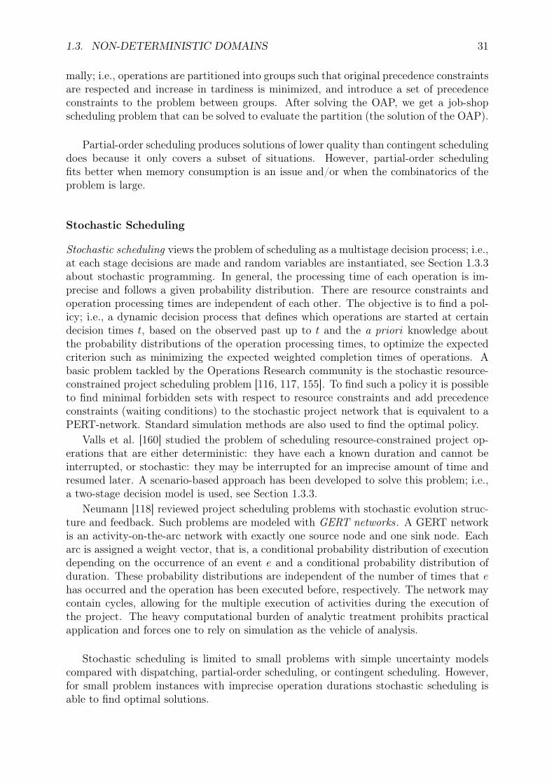
1.3. NON-DETERMINISTIC DOMAINS 31
mally; i.e., operations are partitioned into groups such that original precedence constraintsare respected and increase in tardiness is minimized, and introduce a set of precedenceconstraints to the problem between groups. After solving the OAP, we get a job-shopscheduling problem that can be solved to evaluate the partition (the solution of the OAP).
Partial-order scheduling produces solutions of lower quality than contingent schedulingdoes because it only covers a subset of situations. However, partial-order schedulingfits better when memory consumption is an issue and/or when the combinatorics of theproblem is large.
Stochastic Scheduling
Stochastic scheduling views the problem of scheduling as a multistage decision process; i.e.,at each stage decisions are made and random variables are instantiated, see Section 1.3.3about stochastic programming. In general, the processing time of each operation is im-precise and follows a given probability distribution. There are resource constraints andoperation processing times are independent of each other. The objective is to find a pol-icy; i.e., a dynamic decision process that defines which operations are started at certaindecision times t, based on the observed past up to t and the a priori knowledge aboutthe probability distributions of the operation processing times, to optimize the expectedcriterion such as minimizing the expected weighted completion times of operations. Abasic problem tackled by the Operations Research community is the stochastic resource-constrained project scheduling problem [116, 117, 155]. To find such a policy it is possibleto find minimal forbidden sets with respect to resource constraints and add precedenceconstraints (waiting conditions) to the stochastic project network that is equivalent to aPERT-network. Standard simulation methods are also used to find the optimal policy.
Valls et al. [160] studied the problem of scheduling resource-constrained project op-erations that are either deterministic: they have each a known duration and cannot beinterrupted, or stochastic: they may be interrupted for an imprecise amount of time andresumed later. A scenario-based approach has been developed to solve this problem; i.e.,a two-stage decision model is used, see Section 1.3.3.
Neumann [118] reviewed project scheduling problems with stochastic evolution struc-ture and feedback. Such problems are modeled with GERT networks . A GERT networkis an activity-on-the-arc network with exactly one source node and one sink node. Eacharc is assigned a weight vector, that is, a conditional probability distribution of executiondepending on the occurrence of an event e and a conditional probability distribution ofduration. These probability distributions are independent of the number of times that ehas occurred and the operation has been executed before, respectively. The network maycontain cycles, allowing for the multiple execution of activities during the execution ofthe project. The heavy computational burden of analytic treatment prohibits practicalapplication and forces one to rely on simulation as the vehicle of analysis.
Stochastic scheduling is limited to small problems with simple uncertainty modelscompared with dispatching, partial-order scheduling, or contingent scheduling. However,for small problem instances with imprecise operation durations stochastic scheduling isable to find optimal solutions.

32 CHAPTER 1. STATE OF THE ART
Rescheduling
Rescheduling consists in changing scheduling decisions periodically or when the currentsolution becomes inconsistent; i.e., it is no longer executable. Rescheduling is also nec-essary when the current solution quality changes too much with respect to what waspredicted.
Sabuncuoglu and Bayiz reviewed rescheduling techniques applied to job-shop schedul-ing [139]. They classify approaches with respect to how much we change the predictiveschedule: a full rescheduling consists in changing scheduling decisions of all the pendingoperations; i.e., operations that have not already been executed; a partial reschedulingchanges only the decisions of a subset of pending operations; a local rescheduling, alsocalled scheduling repair, changes decisions of one pending operation.
Sadeh, Otsuka, and Schnelbach [140] worked on a production scheduling problemwhere machines break down. Large Neighborhood Search is used when partially reschedul-ing; i.e., we identify a set of operations to unschedule (“conflict propagation”) by usingrecovery rules and use original scheduling algorithm to reschedule the unscheduled oper-ations.Simple rules are used for identifying the neighborhood and for conflict propagation:
• Right Shift Rule: operations are moved later in time while preserving sequence;
• Right Shift and Jump Rule: operations are moved later in time, jumping over onesthat do not need to be moved.
The idea is to use a simple rule to quickly repair the schedule.When fully rescheduling Micro-Boss is used. Micro-Boss does micro-opportunistic schedul-ing; i.e., it focuses on resource conflicts on limited time period.Opportunistic scheduling has the ability to detect the emergence of new bottlenecks dur-ing the construction of the schedule and change the current scheduling strategy.Macro-opportunistic scheduling is such that an entire bottleneck is scheduled (or at leasta large chunk of it); i.e., it considers resource conflicts over the complete time horizon.Resource contention is always monitored during the construction of a schedule, and theproblem solving effort is constantly redirected towards the most serious bottleneck re-source.During execution dispatching rules are used to adapt schedule:
• Weighted Shortest Processing Time (WSPT);
• Slack per Remaining Processing Time (SRPT);
• Weighted Cost OVER Time (WCOVERT);
• Apparent Tardiness Cost (ATC).
Micro-opportunistic scheduling heuristics are well suited to solving problems in whichsome operations have to be performed within non-relaxable time windows as well asrepairing schedules in the face of contingencies.Using Micro-Boss is a reasonable, pragmatic approach where there is no explicit reasoningabout time to find a solution. There is no reasoning about perturbation but the numberof operations to reschedule is important.

1.3. NON-DETERMINISTIC DOMAINS 33
Another work of interest about partial rescheduling was done by Smith [151]. OPIS isa full scheduling system based on repeatedly reacting to events. It is a more sophisticatedreasoning mechanism for analysis of conflicts than Micro-Boss on the basis of constraintpropagation. This approach to incremental modification management of schedules is basedon a view of scheduling as an iterative, constraint-based process.
El Sakkout and Wallace used a different approach to fully reschedule [141]. Theirapproach consists in a minimal perturbation rescheduling. Given a predictive scheduleand a reduction in resource capacity, we have to find a schedule which minimizes the sumof absolute deviations from operation start times in the predictive schedule.The main idea is to use a hybrid Linear Programming / Constraint Programming branch-and-bound technique because a hybrid approach is better than pure CP and pure MIP.The cost function for measuring change involves some kind of earliness/tardiness which isusually well solved by a MIP approach. One represents temporal constraints and the costfunction in an LP and temporal constraints and resource capacity constraints in CP. Oneuses the relaxed optimal start times from the LP to drive the CP branching heuristic; i.e.,we add new linear constraints in the linear program when we branch in the decision tree(CP model) and propagate these decisions. This technique is named “Probe BacktrackSearch.”Experiment consists in one (non-unary) resource with a given schedule; when an eventreduces resource capacity over some time interval we reschedule.This method is only practical in situations where the time-to-solve is irrelevant. Theoptimization criterion of the original schedule is ignored.
Branke and Mattfeld tackled dynamic job-shop scheduling problems by making deci-sions on a rolling-time horizon [36]. Operation durations are deterministic but jobs arrivenon-deterministically over time. Each job is associated with a due date and the goal isto minimize the summed tardiness. An evolutionary algorithm is implemented to findschedules with short makespans and low early idle times. The generation-execution pro-cess proceeds as follows. An initial schedule is created with the set of known jobs andthe execution of this schedule begins. At some point a new job arrives. All the alreadyexecuted and in process operations are removed from the scheduling problem, the new jobis added and a new solution is found by changing some decisions. When the final activityin a job executes, the contribution to the summed tardiness is calculated.
Shafaei and Brunn published an empirical study of a number of dispatching rules onthe basis of a rolling-time horizon approach for a dynamic job-shop environment [145].Operation processing times are imprecise and randomly picked with equiprobability inranges. Job arrival rate follows a Poisson distribution and shop load is either heavy ormoderate. A release and a due date are associated with each job. The performancemeasure considered is an economic objective. The objective is then to minimize the costof starting jobs too early and the cost of work in progress inventory and tardiness. Thefirst purpose of the study is to find the best dispatching rule and the second to investigatethe effects of the rescheduling interval on performance and examine whether there is apolicy that can always improve performance. In general, under tight due-date conditions,the rescheduling interval has a much more significant effect on performance than underloose due-date conditions: the smaller the interval, the lower the cost.
In another report, Shafaei and Brunn investigate how reliable these dispatching rulesare in a dynamic and non-deterministic shop environment [146]. The number of opera-tions per job is uniformly sampled, job routes are randomly selected, operation processing

34 CHAPTER 1. STATE OF THE ART
times are imprecise, and machines can break down: machine breakdown intervals andrepair times follow exponential probability distributions. The simulation results, undervarious conditions in a balanced and unbalanced shop, are presented and the effects of therescheduling interval and operational factors including shop load conditions and a bottle-neck on the schedule quality are studied. They conclude that more frequent reschedulinggenerally improves performance in an uncertain situation.
Rescheduling is useful when execution environment is very uncertain and/or the initialproblem is changed during execution. However, rescheduling is costly and produces sub-optimal solutions if time for reasoning is short.
Fuzzy Scheduling
The advocates of the fuzzy operation duration approach argue that probability durationsfor the operation durations are unknown due to the lack of historical data [79]. Asoperation durations have to be estimated by human experts, often in a non-repetitive oreven unique setting, schedule management is often confronted with judgmental statementsthat are vague and imprecise. In those situations, the fuzzy set scheduling literaturerecommends the use of fuzzy numbers for modeling operation durations, rather thanprobabilistic variables, see Section 1.3.3.
Fuzzy PERT-network was presented by Galvagnon [67]. The main problem is to coor-dinate different projects whose decision centers are independent of each other and thereis uncertain and imprecise information because each project is unique and no historicaldata exists. A criticality degree is proposed to express that the possibility of a path tobe critical. Unary resources are shared by projects and allocations can be changed if it isnecessary. Operations are not preemptive and we have to decide when to start operations.The external parameters are negotiable; e.g., arrival dates of material are negotiated. Theobjective is to give explanations when a problem has no solution; i.e., what part of theproblem has to be modified to find a solution.
Geneste and Grabot applied fuzzy logic and possibility theory for modeling impreciseexpert knowledge for managing the part flow; e.g., they focused on releasing or dispatchinglots [72], or they studied the way of forecasting a production plan within a negotiationprocess when orders are uncertain and imprecise [74, 73].
Dubois, Fargier, and Prade applied fuzzy theory to scheduling [54]. They tacklescheduling problems with fuzzy operation durations and try to find a schedule that min-imizes the possibility of performance less than a threshold. Standard search techniquesare used but the constraint-satisfaction requirement is replaced by “reasonably sure thatno constraint will be violated.” This is a realistic approach that lies between acceptingonly schedules that are sure to work and accepting a schedule without taking into accountpossible deviations.
The main advantage of fuzzy scheduling over other approaches is its ability to modeltotal ignorance and vague expert knowledge. However, the counterpart is that selection ofsolutions is trickier since possibility distributions can be interpreted differently dependingon subjective criteria.
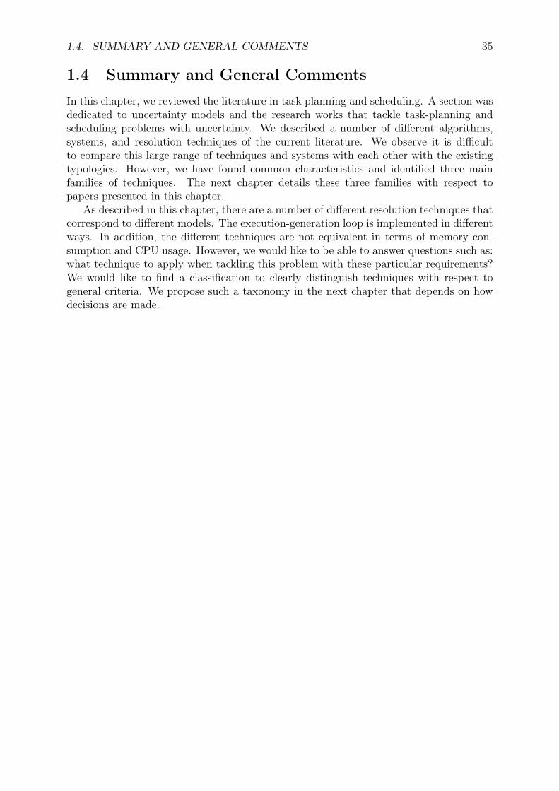
1.4. SUMMARY AND GENERAL COMMENTS 35
1.4 Summary and General CommentsIn this chapter, we reviewed the literature in task planning and scheduling. A section wasdedicated to uncertainty models and the research works that tackle task-planning andscheduling problems with uncertainty. We described a number of different algorithms,systems, and resolution techniques of the current literature. We observe it is difficultto compare this large range of techniques and systems with each other with the existingtypologies. However, we have found common characteristics and identified three mainfamilies of techniques. The next chapter details these three families with respect topapers presented in this chapter.
As described in this chapter, there are a number of different resolution techniques thatcorrespond to different models. The execution-generation loop is implemented in differentways. In addition, the different techniques are not equivalent in terms of memory con-sumption and CPU usage. However, we would like to be able to answer questions such as:what technique to apply when tackling this problem with these particular requirements?We would like to find a classification to clearly distinguish techniques with respect togeneral criteria. We propose such a taxonomy in the next chapter that depends on howdecisions are made.


Chapter 2
General Framework
In this chapter, we propose a classification of techniques for task planning and/orscheduling under uncertainty1 that extends the existing typologies proposed in lit-
erature [44, 28, 161, 85, 94]. The existing classifications are not satisfactory since theyare ambiguous and/or incomplete; furthermore, they usually focus either on AI or ORterminology. Our main motivation for developing such a taxonomy was to structure thecurrent state of the art in a consistent way and allow one to easily classify any algorithmor system. The general framework we present is independent of any specific representa-tion model or reasoning technique. This general classification is focused on decisions; i.e.,a method is classified with respect to how decisions are made. For each family of thisclassification, we give examples reviewed in the preceding chapter. We start this chapterwith discussing some general definitions to avoid ambiguity of terms commonly used indifferent communities. In the second, third, and fourth sections, we introduce revision,proactive, and progressive techniques, and give their definitions. The main idea is thatthere exists a continuum between the purely reactive techniques, where no decision ismade in advance, and the purely predictive ones, where all decisions are made off line; thetechniques that can change all the decisions on line and those that are reluctant to do so;the techniques that take into account uncertainty when making decisions and the tech-niques that do not take uncertainty into account when making decisions, see Section 1.3.We think this continuum can be explored by mixing the three families. The fifth sectionpresents approaches that combine two or more techniques. The last section summarizesthe chapter and contains general remarks about the framework.
2.1 Definitions and Discussion
In task planning/scheduling under uncertainty, we classically define two ways of generatingsolutions: reactive generation and predictive generation. We generate a solution reactivelywhen decisions are made without anticipation on line whereas a predictive solution isgenerated before execution by making all decisions. For example, in scheduling, it iscommon to use simple dispatching rules to make decisions reactively, see Section 1.3.6; itis possible to use the same priority rules for finding a predictive schedule. Notice, however,
1This chapter develops and revisits the work presented in the ICAPS’03 Tutorial on Practical Ap-proaches to Handling Uncertainty in Planning and Scheduling, prepared and presented by Beck andVidal.
37
38 CHAPTER 2. GENERAL FRAMEWORK
that it would be desirable to generate not fully instantiated solutions that are less sensibleto unexpected events and that allow to be less myopic as well.
The first definition concerns a characteristic of a solution.
Definition 2.1.1 (flexibility). A flexible plan/schedule is plan/schedule that is not fullyset; i.e., a subset of decisions DES have still to be made. A plan/schedule s1 is moreflexible than another s2 if the number of possible choices for DESs1 is greater than thenumber of possible choices for DESs2.
There exist different types of flexibility in scheduling that depend on the type ofdecision that still needs to be taken on line [142]. Temporal flexibility lets us decide online when operations start, sequencing flexibility lets us decide on line how operationsallocated to a resource are sequenced, and allocation flexibility lets us choose on line theresource with which an operation will be executed. Notice that in the recent papers theexecution controller commonly decides when to start each operation when allocation andsequencing decisions are made off line. In some cases, there is another type of flexibilitythat is offered; i.e., a subset of operations are chosen on line among a set of alternativesubsets of operations, see contingent scheduling in Section 1.3.6 and conditional CSPs inSection 1.3.5.
Definition 2.1.2 (conditional solution). A conditional plan/schedule, also called contin-gent plan/schedule, is a flexible plan/schedule where alternatives are modeled and only asubset of disjunctions is executed.
There are two kinds of flexibility: either some decision variables of the problem are notinstantiated, all possible instantiations are implicitly expressed, or a number of possibleinstantiations are explicitly expressed. The former flexibility is represented by a partiallyinstantiated solution and the latter flexibility is represented by a set of solutions; i.e., thissolution is conditional.
Reactive task planning/scheduling generates fully flexible solutions because all deci-sions are made without anticipation, see Section 1.3.6 for reactive scheduling. Predictivetask planning/scheduling produces completely instantiated solutions that are not flexible.We can introduce more or less flexibility in the generation process in order to cope withuncertainty and change: there is a trade-off to find between completely flexible solutionsand rigid solutions. A rigid solution can be preferable when it is used by other agents formaking decisions; e.g., a timetable is used by the teacher and students for planning otheractivities than lectures.
The following definitions concern two properties of a solution with respect to uncer-tainty and change.
Definition 2.1.3 (robustness). A robust plan/schedule is a plan/schedule with a qualitythat does not degrade during execution with respect to known on-line perturbations.
We usually introduce some flexibility in plans/schedules when we want to increasetheir robustness. However, a plan/schedule s1 that is more flexible than or as flexible asanother s2 is not necessarily more robust than s2. For example, s1 may be more flexiblethan s2 with respect to deciding operation start times but s1 may have two critical pathswhereas s2 may have only one critical path; in this case it is probable that s1 would be

2.1. DEFINITIONS AND DISCUSSION 39
more brittle than s2, if they were executed in a non-deterministic environment. Noticethat a plan/schedule with a null standard deviation of its optimization criterion (thusthat cannot degrade during execution) but of very bad quality is a robust plan/schedule;e.g., a schedule where all operations are scheduled very far apart is robust.
Robustness is a general term and means different things depending on applicationcontext: it is important to define robustness with respect to a criterion [142] and pertur-bations. Robustness is rather a relative solution property that is usually used to comparetwo or more solutions.
Definition 2.1.4 (stability). A stable plan/schedule is a plan/schedule whose decisionsdo not change during execution. We assume decisions are made with anticipation. Aplan/schedule s1 is more stable than another s2 if s1 changes less than s2 during executionin terms of decisions.
A plan/schedule that is reactively generated is not stable because decisions are notmade in advance, and it is difficult to give guarantees for such a solution with respectto robustness since the optimization criterion is usually computed when a lot decisionsare made and can only be roughly estimated in this case. As defined above, stabilityand robustness are antagonistic optimization criteria; e.g., it is usual to minimize themakespan in scheduling and this is more difficult to do if we also want to minimizethe number of changes whenever we decide to find a new solution during execution tomaintain a high quality. Stability and robustness are always measured after execution.Quality and stability are related in the sense that guaranteeing a very high quality at theend of execution implies maintaining a very high estimated quality during execution, thatis, the baseline solution will be often changed; on the contrary, if we do not care aboutquality but stability is very important, we can generate a solution taking into accountthe worst scenario that may happen during execution and guarantee that these decisionsdo not change (this is a fully predictive schedule). The stability may be defined by thedistance between two schedules; i.e., it depends on the number of different decisions takento generate these two schedules. There are a number of different metrics for assessingrobustness and stability of a schedule in literature [14, 142].
Currently researchers propose predictive-reactive techniques to tackle problems underuncertainty and change; i.e., these techniques generate a first predictive solution and thena new predictive solution is reactively produced whenever the current predictive solutionviolates a constraint. From the research literature, we have identified three possibilitiesto generate solutions when the execution environment is non-deterministic: we take intoaccount uncertainty when making decisions, we change decisions when it is necessary, orwe make decisions on a more or less short gliding horizon. This is a new way of classify-ing task-planning and scheduling techniques and systems that deal with uncertainty andchange, and these three families of techniques are more or less reactive (thus more or lesspredictive), to respond to perturbations that occur at execution time.
Some terms are often mentioned, but not yet standard, so we propose the additionalfollowing definitions.
Definition 2.1.5 (executable plan/schedule). An executable plan/schedule is a plan/sche-dule that does not violate any constraint. Executability of a plan/schedule is a propertythat is checked at a given time instant t.

40 CHAPTER 2. GENERAL FRAMEWORK
A stable solution is always executable because all possible execution scenarios havebeen taken into account during its production, so no constraint will be violated duringexecution.
Definition 2.1.6 (adaptive generation-execution system). An adaptive generation-exe-cution system is a generation-execution system that is able to generate a new executablesolution whenever the current executed solution is no longer executable.
The temporal behavior of uncertain events needs to be further defined to help uscharacterizing a decision-making method.
We know in advance when a synchronous event will occur in relation with other events;i.e., we know in advance it will occur at a precise stage of the plan/schedule. However,we do not know in advance and precisely when an asynchronous event will occur. Anasynchronous event can occur at any time during execution and its occurrence is notsynchronized with other events. For example, observing the outside temperature when anoperation ends is a synchronous event since it occurs synchronously with the end time ofan operation, even if the operation duration is imprecise. Observing the outside pressureat 10:00 P.M. is a synchronous event since we know exactly when it occurs. However,a machine breakdown start time is usually considered as an asynchronous event becausewe do not know in advance the precise plan/schedule stage of its occurrence or its exactoccurrence time.
2.2 Revision TechniquesIn this section, we discuss some general aspects of revision techniques and how they areapplied in scheduling and task planning with examples.
2.2.1 Generalities
Revision techniques consist in changing decisions during execution when it is necessary;e.g., we change decisions when the current predictive solution becomes inconsistent, whenestimated quality deviates too much from the predicted one, or when a positive eventoccurs (for example, an operation finishes very early, or after taking a photo of a landscape,it is decided to move an autonomous robot towards a specific area to do additional scientificexperiments, so we change the current predictive plan by inserting some actions) and wetake advantage of this to optimize.
Definition 2.2.1 (revision decision-making process). A revision technique is able tochange decisions of a solution during execution.
Figure 2.1 represents the generation-execution loop when using a revision technique.The execution controller is in charge of activating actions with respect to the solution itgets and deciding if the current solution must be adapted or changed completely when itobserves a failure or an opportunity event. In addition, the execution controller updatesthe clock.
The on-line revision can be limited or not; i.e., the predictive solution is partially orcompletely changed, respectively. In task planning and scheduling, we are used to theso-called replanning and rescheduling, respectively, when completely changing decisions.

2.2. REVISION TECHNIQUES 41
Plan/Schedule
(Re)planning/
(Re)scheduling
Adapt
off line
on line
real world
Actions
solution execution
Events
Execution controlling
update
failure or opportunitydetection
modify
Figure 2.1: Generation-execution loop with a revision technique.
A predictive schedule or plan executes while nothing unexpected happens; otherwiseit is revised.
In general, reasoning is costly and solutions are usually sub-optimal due to real-timeconstraints that forbid complete optimal replanning/rescheduling search. Revision tech-niques are thus generally implemented by greedy or local search algorithms with ad hocheuristics to quickly find a solution. Such algorithms are often anytime; i.e., they are ableto exhibit a solution whenever search is stopped, and solution quality is improved as longas search continues. For example, local search (repair-based) replanning can be used tofind a predictive plan as close as possible to the previous predictive plan.
One of the issues with such an approach is that it is not always clear when to change thecurrent predictive solution, and it is not always desirable to revise the current predictivesolution frequently. There is thus an issue when solution stability is important. This isthe reason why, in some cases, it is important to design a system for monitoring executionand indicating when to change decisions.

42 CHAPTER 2. GENERAL FRAMEWORK
2.2.2 Examples of Revision Techniques in Task Planning andScheduling
In task planning, we classically face two types of failures when executing a plan in a non-deterministic environment. “Low-level” failures with resource usage or slight delays requirebasically partial rescheduling; i.e., local changes are done when partially rescheduling.When harder failures are observed, we need deeper replanning and a straightforwardapproach is often used:
1. put the physical process, such as an autonomous robot, in a “safe state;”
2. call the deliberative planner for a new plan;
3. wait for the new plan;
4. restart execution.
There are different approaches to replan, see Section 1.3.5 devoted to continuous plan-ning. We can resolve quickly and myopically by using rules, partially resolve with LargeNeighborhood Search or specialized heuristics, or fully resolve. Time pressure and solu-tion quality requirements largely determine the approach applied: rule-based methods forfinding quickly sub-optimal solutions, or minimal perturbation techniques when you haveenough time.
In scheduling, the revision method consists in executing one predictive schedule, andduring execution if something goes wrong; e.g., a machine breaks down, then repairingthe predictive schedule so execution can continue. Such a revision procedure is calledrescheduling. In some applications, revision is done periodically.
Notice that the revision method is usually called predictive-reactive in literature [139,94].
A preceding section 1.3.6, dedicated to rescheduling, has presented some relevantpapers about revision scheduling [139, 140, 151, 141].
2.2.3 Discussion
Revision techniques are always useful in strongly non-deterministic environments in whichasynchronous events and/or low probability events can happen.
Not much memory is needed to store a solution but the search process might need largerspace in addition. However, if we use a case-based reasoning technique this requires tostore information about past experiences but the search process is not expensive in termsof memory consumption since we only have to find the past solution that matches bestthe current situation.
2.3 Proactive Techniques
In this section, we discuss some general aspects of proactive techniques and how they areapplied in scheduling and task planning. This section is devoted to techniques that takeinto account uncertainty to produce robust solutions that are more or less flexible, and try

2.3. PROACTIVE TECHNIQUES 43
to reduce the brittleness of the solutions produced by purely revision generation-executionprocesses. A pure proactive technique generates a solution that will not be revised duringexecution since it is not sensitive to perturbations.
2.3.1 Generalities
A proactive technique takes into account uncertainty to produce solutions that are lesssensitive to perturbations that occur on line. The generation procedure takes into accountuncertainty if information about uncertainty is present; e.g., uncertainty is modeled withdistributions. However, information about uncertainty is not always available even ifwe know that unexpected events can occur during execution. For example, Hebrard,Hnich, and Walsh presented recently some work on constraint-satisfaction problems, seeSection 1.2.4, in which they propose proactive search algorithms that find super solu-tions [82]. Super solutions are solutions that can be easily repaired if they are perturbedto some extent; i.e., if a limited number of assignments are changed simultaneously in asupersolution we can find a new solution by changing a limited number of other assign-ments.
One possible method, the rigid proactive approach, for making a solution insensitiveto on-line perturbations is to produce a predictive, robust solution, such that all itsdecisions are made off line by taking into account the worst scenario that can happenduring execution.
We propose a new term when planning tasks or scheduling with a proactive technique:maximal coverage consists in assessing the level of feasibility or optimality of the planknowing the probability, possibility, or plausibility of deviations Pdev. We try to find theplan that minimizes Pdev; i.e., we try to provide one and only one plan that is expectedto work or to have a quality greater than a given threshold “most of the time,” for asatisfaction problem and for an optimization problem respectively. Maximal coverage canbe combined with a revision technique; i.e., a robust plan is proactively generated andrepaired when it is not any more executable or optimal.
Fargier et al. proposed a constraint-satisfaction framework for making decisions underuncertainty with a fuzzy, maximal coverage approach [62]. Similarly, when dealing withProbabilistic CSPs, we are looking for the solutions such that the probability that each ofthem is consistent with the actual set of constraints is maximized or greater than a giventhreshold, see Section 1.3.3.
Another approach, the flexible proactive approach, consists in introducing some flex-ibility in the solution produced off line; i.e., some decisions are not made off line butreactively on line and they are not taken too early; this is a kind of least commitmentapproach with respect to decision-making since we only make decisions when informationis more complete, more precise, and/or more certain. During the execution of such a flex-ible solution, a synchronous event occurs; e.g., the execution of an operation finishes or aninformation gathering is done, and there are two possible ways of making the remainingdecisions depending on the kind of flexibility used. We distinguish continuous flexibilityfrom discrete flexibility in the remaining of the document and define them as follows:
• continuous flexibility: we can make new decisions to complete the current flexibleplan/schedule2 given an execution policy; i.e., we make the flexible solution more
2Continuous flexibility can be obtained by introducing temporal flexibility, allocation flexibility, and/or

44 CHAPTER 2. GENERAL FRAMEWORK
rigid;
• discrete flexibility: we observe conditions and match observations to next opera-tions/actions; i.e., a subset of operations is thrown away while others are kept andpossibly executed3.
A flexible proactive method generates a flexible solution without enumerating all pos-sible predictive solutions it contains whereas a discrete proactive technique explicitlyproduces a number of predictive solutions.
Definition 2.3.1 (proactive decision-making process). A proactive technique is able toproduce solutions that are as insensitive to on-line disruptions as possible.
Figure 2.2 represents the generation-execution loop when using a proactive technique.The execution controller is responsible for updating the clock, making the remainingdecisions when the solution is flexible, and activating actions.
When information about unexpected events is available we use for example a proba-bilistic or fuzzy representation of uncertainty to generate a plan/schedule that will coverall cases; e.g., the plan/schedule will run without any problem in 100% of cases even if itis still a predictive plan/schedule. Notice that, in general, the solution of such a proactivegeneration process is completely stable, it is a robust solution but sub-optimal.
An extreme proactive generation system consists in finding the predictive optimal so-lution of each deterministic problem corresponding to a possible realization of the randomvariables. This is impossible to apply such a method to a practical problem because ofthe huge time and memory space that would be used. For example, we consider MarkovDecision Processes, see Section 1.3.3, as a proactive technique because all possible statesof a process are represented, however, optimal decisions are not made because the decisionmade at a given time only depends on data about past and the reward associated withbeing in the next state, and does not take into account the whole combinatorial problem,in particular, information about future.
An algorithm that checks controllability is a proactive technique that filters control-lable decisions that can lead to a non-executable solution, see Section 1.3.4.
Without any knowledge about perturbations we can not generate solutions proactively.
2.3.2 Examples of Proactive Techniques in Task Planning andScheduling
Proactive planning generates robust plans; i.e., robust plans are the plans that maximizethe chance of reaching the goal state given knowledge about uncertainty. This can bedone assuming a closed loop execution if generated flexible plans are contingent ; i.e.,decisions on what actions to execute next are based on observations. Contingent planning,also called conditional planning or state-based planning, is a way to plan proactively,see Section 1.3.5. Partial observability is sometimes imposed and we have to deal withuncertain observations; probabilistic planning is a convenient approach in these cases, seeSection 1.3.5.
sequencing flexibility in the solution, see [27].3Discrete flexibility can be obtained by introducing mode flexibility in the solution, see [27] and
conditional planning in Section 1.3.5.

2.3. PROACTIVE TECHNIQUES 45
Planning/Scheduling
off line
on line
real world
Actions
update
solution execution
scheduleplan/
Flexible
Events
Execution controlling
Figure 2.2: Generation-execution loop with a proactive technique.
At one extreme, there are cases where observation is not possible at all and we haveto use conformant plans; i.e., predictive plans that guarantee to attain the goal statewhatever happens during execution, see Section 1.3.5. Note that conformant planningimplies that we have a closed loop execution.
• The research work of Dubois, Fargier, and Prade is a good example of proactivescheduling with using fuzzy logic [54], see Section 1.3.6.
• Just-In-Case scheduling is a proactive technique par excellence, see Section 1.3.6.
• Redundancy-based scheduling is also considered as a proactive technique, see Sec-tion 1.3.6.
• Generating partial-order schedules (POSs) is a proactive scheduling technique sincea subset of sequencing decisions are made off line and the remainder being made on
46 CHAPTER 2. GENERAL FRAMEWORK
line with using a dispatching rule, see Sections 1.3.6 about POSs and 1.3.6 aboutdispatching rules.
2.3.3 Discussion
A revision technique is usually combined with a proactive approach to cover situationsthat occur rarely and that are not taken into account by the proactive approach; e.g.,a river flooding is usually a low probability event, see Section 2.5 dedicated to mixedtechniques.
2.4 Progressive Techniques
In this section, we discuss some general aspects of progressive techniques and how theyare applied in scheduling and task planning with examples.
2.4.1 Generalities
The idea behind progressive techniques is to interleave planning/scheduling and execu-tion, by solving the whole problem piece by piece. Reasoning is done off line and as abackground task on line; i.e., we can afford more time to search, we incrementally committo scheduling/planning decisions periodically or when new information arrives, and nodecision is changed.
Definition 2.4.1 (progressive decision-making process). A progressive technique is ableto incrementally make decisions off and on line.
Figure 2.3 represents the generation-execution loop when using a progressive tech-nique. The execution controller has the responsibility to update the clock, activate ac-tions, and decide when it is useful or necessary to make new decisions.
One way of proceeding when using a progressive approach is to select and plan/schedulenew actions/operations to possibly extend the current executing solution when an eventoccurs. This event brings information that is integrated and propagated in the currentplan/schedule. Whereas revision and proactive techniques possibly change/make all de-cisions of the problem at the same time and by reasoning on the whole problem, we focuson sub-parts of the problem when progressively generating a solution. When using aprogressive approach, the solution is produced piece by piece: we have to select a subsetof decision variables, on which we make decisions. In addition, we have to select a subsetof data from which we reason because it is senseless, indeed dangerous to make decisionswhen the data from which we reason are too uncertain.
A solution produced by a progressive technique is sub-optimal since decisions are takenonly with a more or less short-term/aggregated view; i.e., they are made locally or witha rough estimation of the whole problem. A decision is made when uncertainty levelof the used information is not too high and/or time before execution of this decisionis too short; this assumes there is an execution monitoring system able to react andindicate when and what type of decisions to make. However, such a technique can alsobe used periodically without having to monitor execution. One of the advantages tousing progressive techniques is that not much memory is needed for storing a progressive
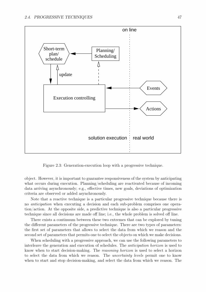
2.4. PROGRESSIVE TECHNIQUES 47
Planning/Scheduling
scheduleplan/
Short-term
real world
Actions
Events
solution execution
Execution controlling
update
on line
Figure 2.3: Generation-execution loop with a progressive technique.
object. However, it is important to guarantee responsiveness of the system by anticipatingwhat occurs during execution. Planning/scheduling are reactivated because of incomingdata arriving asynchronously; e.g., effective times, new goals, deviations of optimizationcriteria are observed or added asynchronously.
Note that a reactive technique is a particular progressive technique because there isno anticipation when executing a decision and each sub-problem comprises one opera-tion/action. At the opposite side, a predictive technique is also a particular progressivetechnique since all decisions are made off line; i.e., the whole problem is solved off line.
There exists a continuum between these two extremes that can be explored by tuningthe different parameters of the progressive technique. There are two types of parameters:the first set of parameters that allows to select the data from which we reason and thesecond set of parameters that permits one to select the objects on which we make decisions.
When scheduling with a progressive approach, we can use the following parameters tointerleave the generation and execution of schedules. The anticipation horizon is used toknow when to start decision-making. The reasoning horizon is used to select a horizonto select the data from which we reason. The uncertainty levels permit one to knowwhen to start and stop decision-making, and select the data from which we reason. The

48 CHAPTER 2. GENERAL FRAMEWORK
commitment horizon is used to know when to stop decision-making. The anticipationhorizon is the time period between the current time and the next time we will have tomake and execute new decisions without anticipation; i.e., when the anticipation horizonbecomes too small, we have to make new decisions to keep the lead of decision-making overexecution. The reasoning horizon is the gliding-time period on which we select the datafrom which we reason. The uncertainty levels are reference thresholds indicating whenwe can make new decisions, what sub-problem to tackle with respect to the uncertaintylevels of its operations/actions, and what data to use when reasoning for making newdecisions. The commitment horizon defines the gliding-time period in which decisions aremade. This is greater than the anticipation horizon; e.g., we make decisions for the nexttwo days (commitment) and make new decisions every day (anticipation). The reasoninghorizon is equal to or greater than the commitment horizon; e.g., we reason from the dataof one week but make only decisions for the next two days. Table 2.1 summarizes theroles of these parameters.
Start Stop Select the datadecision- decision- from whichmaking? making? we reason?
Anticipation horizon Yes No NoReasoning horizon No No YesUncertainty levels Yes Yes Yes
Commitment horizon No Yes No
Table 2.1: The basic parameters of a progressive approach.
2.4.2 Examples of Progressive Techniques in Task Planning andScheduling
Progressive planning consists in updating and completing the current plan by adding newactions.
Continuous planning is a progressive approach par excellence when no replanningoccurs [120], see Section 1.3.5 for more details. The plan is built piece by piece duringexecution.
There is another approach, called telescoping-time horizon, that consists in generatinga global plan, but it is more detailed in the short range than in the long range, see someworks done at NASA Jet Propulsion Laboratory [40, 59]. The idea is to maintain anincomplete or abstract plan in the longer range. The plan is thus further detailed asexecution progresses.
There is less work dealing with progressive approach in scheduling than in planning.Usually, schedules are periodically completed; e.g., we make new decisions every two days.A short-term schedule on which decisions are made is sometimes called an “overlappingplan” in manufacturing. Some works use a progressive approach combined with a revisionmethod [36, 145, 146], see Section 2.5.2.
Vidal, Ghallab, and Alami worked on a scheduling problem by using a progressive ap-proach because of imprecise temporal requirements [167], this is detailed in Section 1.3.4.

2.5. MIXED TECHNIQUES 49
2.4.3 Discussion
It should be noted that a progressive technique is a compromise between purely reactiveand purely predictive techniques. Purely reactive techniques are dispatching techniques;i.e., we use a reactive approach when we only schedule the next operation that has notyet executed on each resource. Purely predictive techniques make all decisions off line:they make decisions in the long term. The larger the horizon, the more predictive; thesmaller the horizon, the more reactive.
A progressive approach is useful when the uncertainty level is high and/or memoryconsumption is limited. A partial solution requires less space than a complete solutionof the same problem and the search space associated with a partial problem is smallerthan the search space associated with the corresponding whole problem. A progressiveapproach is particularly suitable for dynamic problems.
2.5 Mixed Techniques
In this section, we discuss some general aspects of mixed techniques; i.e., mixed methodsare the methods that combine two or more pure solution-generation methods: revision,proactive, and progressive techniques. We explain how they are applied in scheduling andtask planning with examples.
2.5.1 Generalities
There is not a lot of work presenting mixed techniques but this is becoming more at-tractive. Mixed techniques try to respond to various needs such as: limit the memoryblow-up induced by some proactive techniques that explicitly store a lot of alternative pre-dictive solutions, handle unavoidable failures and handle them better. About the latterpoint proactive and progressive techniques restrict the need to revise, hence more effortis dedicated to unforeseen events that are called risks.
Figure 2.4 gives a global view of the general framework. The revision, proactive,and progressive techniques permit the exploration of the continuum that exists betweenpure reactive and pure predictive techniques. The proactive method can generate robustsolutions because it takes into account uncertainty information, the revision approachcan change some of the non-effective decisions of the current solution when it is no longerexecutable, and the progressive technique can generate solutions piece by piece duringexecution. With a pure rigid proactive approach, we can generate predictive solutions.
With a pure progressive approach, we can set the commitment horizon to obtain anapproach that is more or less predictive (more or less reactive): when the commitmenthorizon is very short, the approach is reactive, and, when the commitment horizon is verylong, the approach is predictive.
This is also possible to generate predictive solutions and modify them when they areno longer executable with a revision approach. In case we use a flexible proactive solution,we have to adapt the flexible solution with respect to what is observed during execution.
The number of possible combinations of these three families of techniques is huge andallows the creation of any generation-execution technique.
We actually need to put together all pure solution-generation methods since they arecomplementary. The revision techniques are unavoidable because we are not omniscient

50 CHAPTER 2. GENERAL FRAMEWORK
generate and adaptproactive
revisiongenerate and modify
progressivegenerate and complete
reactive predictive
Figure 2.4: A global view of the general framework.
and an unexpected event can always occur on line. The proactive techniques limit thefrequency of on-line reasoning and offer guarantees on the quality of solutions.
The main interest of progressive techniques is twofold: we ensure a certain stability(when compared with revision techniques) and they are computationally cheaper thanthe approaches that reason with the complete problem over the complete horizon. Therevision-progressive techniques limit the memory blow-up of conditional solutions. Thisis one of the motivations for the theoretical model proposed in Chapter 4. Figure 2.5represents the generation-execution loop when using a mixed technique. The executioncontroller is in charge of updating the clock, choosing and/or activating actions given anexecution policy, deciding when to adapt, change or complete the current partial solutionby observing events.
Table 2.2 is a synthesis of the different properties of each family of solution-generationtechniques used to handle uncertainty and/or change.
A revision method requires a high computational effort on line since decisions arechanged by reasoning but the memory consumption is medium since we only store onesolution and require memory if we use a search tree when looking for a solution. A revisiontechnique is useful when unexpected events can occur; e.g., when a machine breaks downwe usually need to use a revision technique to change allocations. A revision techniquedoes not generate high-quality solutions since there are usually real-time requirements.
A pure proactive method aims at generating solutions whose decisions are not changed

2.5. MIXED TECHNIQUES 51
Adapt
(Re)planning/(Re)scheduling
Execution controlling
off line
on line
modify
detectionfailure or opportunity
update
real worldsolution execution
Events
Actions
Short-term and/
plan/scheduleor flexible
Figure 2.5: Generation-execution loop with a mixed technique.
during execution. The more accurate the uncertainty knowledge, the more efficient theproactive technique. A flexible proactive technique does not require a lot of memory on linesince only one flexible solution is recorded and used. The computational effort requiredon line is low because most of decisions have been made off line and the rest is only basicdecision-making, such as deciding when to start operations. The solutions generated bya flexible proactive generation process are of high quality since the most critical decisionshave been made off line when there are not real-time constraints. A discrete proactivemethod requires a lot of memory since a large number of fully instantiated solutions arerecorded for coping with any possible situation. However, the CPU usage is very low sincethe execution controller only needs to change solutions if the current solution is no moreexecutable or not satisfactorily on line; i.e., only solution matching is done. Theoretically,a pure proactive approach can generate optimal solutions since all possible situations arecovered by recorded solutions generated off line without real-time requirements.
One of the objectives when using a progressive technique is to build a solution incre-mentally without changing decisions. The required memory on line is very limited since

52 CHAPTER 2. GENERAL FRAMEWORK
only a partial solution is stored and the search tree is of reasonable size. However, theon-line CPU usage is medium since sub-problems are solved for completing the currentpartial solution. A progressive approach is not optimal since only a sub-problem is tackledand an estimation of the remaining part is used to make decisions.
On-line On-line Quality Stabilitymemory CPU (optimization
need need criterion)Revision Average High Very high LowProactivecontinuous Low Low High AverageProactivediscrete Very high Very low High Average
Progressive Very low Average Average Very high
Table 2.2: The properties of each family of solution-generation techniques.
2.5.2 Examples of Mixed Techniques in Task Planning and Sche-duling
The literature about mixed scheduling is virtually void.Branke and Mattfeld tackled dynamic job-shop scheduling problems by making deci-
sions on a rolling-time horizon (progressive) and by changing some decisions (revision) [36],see Section 1.3.6. Note, however, that the progressive approach is not chosen by the au-thors but required to solve such a dynamic problem; i.e., no monitoring of execution isused to decide when to select and schedule operations.
Shafaei and Brunn published an empirical study of a number of dispatching rules onthe basis of a rolling-time horizon approach for a dynamic job-shop environment (progres-sive) [145], see Section 1.3.6 for more details. The first purpose of the study is to find thebest dispatching rule and the second to investigate the effects of the rescheduling interval(revision) on performance and examine whether there is a policy that can always improveperformance. In another report, they investigate the robustness of these dispatching rulesin a dynamic and non-deterministic shop environment [146], see Section 1.3.6 for moredetails. The effects of the rescheduling interval and operational factors including shopload conditions and a bottleneck on the robustness of the schedule are studied.
Continuous planning mixes progressive and revision techniques and has been exper-imented by Chien et al. in a space exploration context [40]. Planning is done on boardto speed the replanning process (revision) when a failure occurs or a science opportunityis observed. At each time, the system updates the current plan, goals, state, and nextpredicted states by using a telescoping-time horizon approach (progressive). When a newgoal is up-linked, the current plan is updated. When a plan failure happens, an iterativerepair procedure that uses a greedy search algorithm, is applied in the short-term horizonto change allocations, move, renew, or remove actions. An extension of the system wasproposed by Estlin et al. to manage a team of robots [59], see Section 1.3.5 for moredetails.
Washington et al. used a proactive-revision planning technique for controlling a plan-etary rover with limited capacity resources and uncertainty [173]. A nominal flexible

2.6. SUMMARY AND GENERAL COMMENTS 53
and conditional plan (proactive) is up-linked. Upon failure, short-term recovery plans(revision) can be computed by the state identification module and the resource managerprovides on-board rescheduling capabilities, see Section 1.3.5 for more details.
Lemai and Ingrand proposed a general control architecture that is able to interleaveplanning, replanning (revision) and execution of an autonomous system in an uncertainworld [101, 102], see Section 1.3.5. Partially ordered and partially instantiated plansare generated and allow the insertion of new actions and/or new goals during execution(progressive).
We present an experimental study in Chapter 5 where mixed techniques are used tosolve dynamic scheduling problems with uncertainty.
2.6 Summary and General CommentsIn this chapter, we presented an original typology that can classify research on task plan-ning or scheduling under uncertainty. Three main families of techniques were proposed:a revision approach is able to change decisions on line, a proactive approach makes deci-sions by taking into account uncertainty knowledge, and a progressive approach generatesa solution piece by piece. Each family fits to particular application domains; e.g., ifthe domain is critical, then a revision approach can be desirable to guarantee that anexecutable solution can always be generated whatever happens at execution time. Weargued these techniques can be combined to tackle complex real-world task-planning orscheduling problems.
When designing a decision-making system, it is important to analyze the uncertaintysources of the application in order to know whether we can do with or without a revision,proactive, or progressive technique. As explained earlier in this chapter, this choice de-pends on what can happen during execution, what the physical constraints are in termsof memory and time, and what the requirements are in terms of quality.
The next chapter presents our application domain and shows how these families oftechniques are useful for tackling related problems.


Chapter 3
Application Domain
In this chapter, we present our application domain that is project management. Inparticular, we are interested in the construction of dams.The first section presents concepts of project management and project scheduling.
The second section describes how the construction of a dam is carried out and its sourcesof uncertainty. An example of project scheduling problem is detailed in Section 3.2.3.
3.1 Project Management and Project SchedulingProject management is a management discipline that is receiving a continuously growingamount of attention [89, 110]. There are a number of industrial and service domains whereorganization and work are based on projects; e.g., software engineering, civil engineering,research-and-development are organized on the basis of projects. A project is similar toa scheduling problem since it comprises a set of activities that have to be executed usingresources with limited capacities and given precedence relationships. Project managementconsists in selecting, organizing in time, and controlling the activities and resources of theproject. Project scheduling , as part of project management, has the objective of (i) settingthe activity start times and (ii) allocating resources to activities. There are a lot of projectsthat fail because they are not finished on time, do not respect specifications, and/or theyexceed their budgets.
Budget is exceeded when management deliberately decides to speed up the projectexecution; e.g., additional resources are bought and/or overtime is done. Costs can alsoincrease due to unforeseen event; e.g., some activity durations are longer than expectedsuch that resources are required longer than initially planned, new resources are requiredsince the current resources are not sufficient to meet project needs. Such risks are eithercompletely unpredictable and a revision technique is strongly desirable to handle them,see Section 2.2, or they are foreseeable and can be taken into account by a proactivetechnique to limit their negative effects on budget, time, and/or quality, see Section 2.3.
Project management can be seen as a continuous planning-monitoring-controlling pro-cess, where some data are gathered and used to compare the observed progress to theinitial plan and some repair actions are performed in case of deviation [110]. This mo-tivates the design and use of an execution-generation system that monitors execution,completes and/or revises the current plan to maintain and optimize its cost (budget), itstime (schedule), and its performance (specifications). The main difficulty when designingsuch a system is to precisely choose which specific characteristics of cost, time, and per-
55

56 CHAPTER 3. APPLICATION DOMAIN
formance should be monitored and controlled, and within which bounds they should bemaintained.
Notice that a project can be partitioned into several sub-projects that are executedone after another given intermediate milestones. A progressive approach can then beapplied to quickly generate a plan piece by piece (a piece is the solution of a sub-project)and avoid too frequent revisions (stability).
The above presentation of project management and project scheduling confirms ouridea that we need to monitor and control execution by mixing different scheduling tech-niques to cope with uncertainty when managing a project, see Section 2.5. In the nextsection, we will illustrate this idea with an example of the construction of a dam wall.
3.2 Construction of Dams
In this section, we describe how the project for constructing a dam unfolds. The mainsources of uncertainty are given and a small example that illustrates a scheduling problemunder uncertainty is proposed at the end.
3.2.1 General Description
During the Ph.D. thesis, we have been in contact with a Moroccan civil engineeringcompany, Société Générale des Travaux du Maroc (SGTM), who is in charge of designingand building dams.
In a typical project, SGTM receives a contract specifying the budget, the constructionsite, the main tasks to perform, about twenty intermediate milestones, and the finaldue date. Usually, such a project lasts about three years and some tasks are due atintermediate milestones, otherwise SGTM must pay penalty costs that depend on howlate tasks are completed. The project for constructing a dam usually takes place asfollows:
1. roads are constructed to go easily from one place to another in the building site;
2. prefabricated houses for workers are built;
3. a tunnel for diverting water is dug, this tunnel has to be operational before a duedate determined by the hydrological flow of the river;
4. the dam foundations are prepared for supporting the dam wall, it is probable thatthey need to be later consolidated by injecting cement in particular places but wedo not know when and where before observing the dam-wall conditions;
5. the wadi, that is, the river bed, is drained at the place where the dam wall is built;
6. a canal is dug and used to drain mud lying above the dam;
7. the dam wall is constructed, a tunnel is dug under it and used to observe the dam-wall conditions, and upstream and downstream reinforcements are constructed;
8. the diversion tunnel is blocked.

3.3. GENERAL COMMENTS 57
The civil engineering company can agree or disagree to build the dam under thecontractual constraints.
If an agreement is reached, then a plan has to be generated and maintained by SGTM.The main objectives of the plan are the following: managing risks and having earlywarnings the plan may go wrong. For these reasons, SGTM is interested in using softwarecapable of automatically producing plans that respect the contractual constraints andthat are not sensitive to risks.
3.2.2 Uncertainty Sources
When constructing a dam, we usually have to cope with different sources of uncertainty:
• the water flow of a river changes a lot depending on seasonality. However, somehistorical statistics are available to forecast what the water flow is at given moment;
• vehicles and machines used to construct the dam are not fully reliable and can breakdown. It is possible to use technical data, such as mean time between failures, toguess when a machine will probably be out of service;
• the geological conditions of the place where the dam will be built are not knownwith accuracy before starting the project and can affect the project duration;
• the civil engineering company must interact with another company, specialized inhydromechanics engineering, in charge of installing sheetings at some places in thedam wall. These sheetings are metal frames that will be equipped with floodgatesand hydraulic engines. SGTM cannot continue the construction of the dam wallabove sheetings while they are not installed: there are temporal constraints to re-spect and the installation of sheetings may be finished later or earlier than expected;
• climate is also a source of uncertainty, in particular the outside temperature andhumidity. Workers cannot perform tasks if the outside temperature is too high andtask durations depend on the outside humidity.
3.2.3 An Illustrative Example
There are alternative rough materials for constructing a dam wall. In case a dam wall ismade of concrete, its construction consists in piling up concrete blocks successively. Sucha dam wall is usually composed of about 150 blocks. Blocks are produced by coffering,i.e., some quantity of concrete is poured into a coffer. It is not possible to pile a newblock just to one side or on top of a fresh piled block. Time to dry a block depends onthe outside humidity. In addition, concrete has to be produced at about 20 Celsius andhas to be poured when the outside temperature is less than 30 Celsius.
Figure 3.1 represents a picture from the side of a small concrete dam wall. The 48concrete blocks are numbered.
3.3 General CommentsWhen managing the construction of a dam, we have to cope with uncertainty as explainedin this chapter. There are actually several stages when constructing a dam that are

58 CHAPTER 3. APPLICATION DOMAIN
48 47 46 45 44 43 42 41
33 34 35 36 37 38 39 40
32 31 30 29 28 27 26 25
19 20 21 22 23 24
131415161718
7 8 9 10 11 12
6 5 4 3
21
wadi
sheeting
Figure 3.1: An illustrative example of a concrete dam wall.
dependent on weather and/or geological conditions; e.g., the hydrological flow of theriver and outside temperature are not controllable and imprecisely known and play animportant role when making decisions all along the project. In such a context, we needa revision technique since there are unexpected events that may occur; e.g., a truck maybreak down and we have to use another one. When generating a schedule for such aproject, we can take into account statistical data to make it more robust with respectto possible perturbations; e.g., if the outside temperature is forecast to be greater than30 Celsius for a week, we can decide in advance to postpone some activities that mustbe performed when the outside temperature is less than 20 Celsius. In addition, it issenseless to schedule activities three years in advance since a lot of unexpected eventsmay occur in the meantime: we need to schedule with a progressive technique that is ableto complete the current schedule on the basis of the uncertainty level; e.g., a schedule isgenerated for a horizon of four weeks and is updated every week. This periodicity canchange depending on what construction stage is currently done; e.g., the period is shortif the uncertainty level associated with the current construction stage is high.
When generating a schedule in such a context, we have to take into account alternativeprocesses; i.e., there are sometimes different possibilities to perform a stage. For example,the diversion tunnel can be built in two different ways depending on geological and weatherconditions observed during the construction of roads, so required machines are differentand the duration necessary for building the diversion tunnel depends on what machinesare used. It is also desirable to provide the decision-maker with a flexible schedule in which

3.3. GENERAL COMMENTS 59
alternatives are implicitly and explicitly represented, that is, decisions are not made tooearly because we do not want to make the solution too brittle, some alternatives aredecided based on observations during execution, and some decisions are made based onexpert knowledge that is difficult to represent and process automatically; e.g., operationstart times are not set in advance or operations to execute are not chosen in advance. Sucha flexible solution can be useful to decide when to make decisions to anticipate execution.
Figure 3.2 is a model representing a part of a dam-construction project. Each operationis represented by an arc such that the source of the arc represents its start time and thetarget of the arc represents its end time. There are temporal constraints, represented byarcs, between operations; e.g., we cannot drain the wadi, modeled by o11, before preparingthe foundations, modeled by o9. Some operations are executed in parallel with others;e.g., we build houses, modeled by o5 and o6, while constructing some roads, modeled byo4. Alternatives are also represented; e.g., the construction of the draining canal canbe performed in five ways, modeled by operations of S2. We decide what operations toexecute based on what weather and geological conditions are observed when starting todrain the wadi, modeled by o11, and when the observation tunnel is finished, modeled byo10. This example is presented in detail in the next chapter.
Herroelen and Leus argue that we need a baseline schedule when dealing with multi-project scheduling problems since a baseline schedule is stable and desirable to coordinateseveral projects that are interdependent [103, 84]. They are looking for a schedule thatis able to suppress the propagation of disruptions. In particular, they want to minimizeexpected deviations in starting times. It is very important for them to find a stableschedule since a perturbation may impact the schedules of all projects otherwise.
However, in the context of dam construction, stability is of interest but not the pri-ority because there is only one project and few interactions between SGTM and othercompanies. We are searching for schedules that minimize the probability or the possibil-ity that the expected cost is greater than the initial budget, in other words, we want toguarantee a service level. We are looking for trade-off solutions with maximal robustnesswith respect to costs and with minimal expected costs.
In the next chapter, we detail our theoretical model that can be used to design ageneration-execution model for tackling scheduling problems with uncertainty, such asdam-construction projects.

60 CHAPTER 3. APPLICATION DOMAIN
S2
S3
o11 o9
o10
o6o5
o4
Figure 3.2: Simple temporal representation of a dam-construction project.

Chapter 4
Theoretical Model
This chapter presents the first steps towards a generic theoretical model that allows oneto describe the generation and execution of schedules in a non-deterministic envi-
ronment. This model is directly related to the general framework presented in Chapter 2because it integrates revision, proactive, and progressive techniques. When making deci-sions in a non-deterministic environment, it is crucial to know when to make decisions,what information to use to make decisions, and what decisions to make. This schedulegeneration and execution model is intended to help answer these questions when dealingwith a dynamic scheduling problem with uncertainty. Some preliminary research workhas already been published in French [165, 163].
The first section of the chapter describes the model expressivity with a list of problemcharacteristics that can be addressed. The second section is dedicated to defining formallythe main components of our generation-execution global model, starting from a genericmodel of the schedule patterns that we wish to build and monitor. The third sectionshows how the generation-execution model is developed on line. The last section presentsa toy example to illustrate our theoretical model.
4.1 Model Expressivity
The proposed theoretical model is designed for application to deterministic and non-deterministic problems. This model can process a large range of scheduling problems.The problem characteristics that we can address with this model are as follows:
• an operation can require one or more resources with different quantities, an operationcan also require that a resource is in a given state to execute;
• a resource can be discrete, and/or characterized by a state function and/or anefficiency function (the processing times of the operations depend on resource effi-ciencies);
• there can be delays and/or precedence relationships between operations;
• it is possible we do not know precisely the processing time of an operation in advance;this processing time is a random variable associated with a distribution over itsdomain, this can be either a probability distribution or a possibility distribution;
61

62 CHAPTER 4. THEORETICAL MODEL
• resource capacities, states, and efficiencies can change over time and can be associ-ated with distributions;
• there can be operations that are mutually exclusive; i.e., only a subset of the oper-ations that are mutually exclusive will be executed, that is related to a particularcondition that will be met during execution; such a condition may be associatedwith a probability or possibility distribution; for example, we execute a subset ofoperations because the outside temperature at 9:00 A.M. is lower than 30 Cel-sius; we would execute another subset of operations if the outside temperature wasstrictly higher than 30 Celsius and lower than 40 Celsius at 9:00 A.M.; if the tem-perature was strictly higher than 40 Celsius at 9:00 A.M. we would not execute anyoperation: one can clearly note that this feature of our model is directly inspired byconditional planning techniques, and related to the discrete proactive approaches,see Section 2.3.1.
• there can be an optimization criterion;
• the problem can change over time: new operations can be added or removed, dis-tributions can change, resource capacities, states and efficiencies can change, andtemporal and resource requirements can change.
Figure 4.1 represents the temporal part of a problem that can be handled by ourmodel. Operations are represented by arcs labeled with their processing time domains;e.g., operation o7 has a processing time domain [pmin
7 , pmax7 ]. Temporal requirements are
represented by arcs; e.g., there are temporal requirements between the end time of op-eration o1, end1, and the start time of operation o2, start2. The figure represents anAND/OR directed graph because some nodes separate mutually exclusive subsets of op-erations. Conjunctions are represented by arcs connected with small arcs of a circle; e.g.,operations o4 and o5 might be executed in any order or in parallel. Disjunctions arerepresented by arcs that are not connected with arcs of a circle; e.g., operations o12 ando13 are mutually exclusive. Disjunctions can represent the different ways of attaining agoal; e.g., the different possible ways of producing a workpiece given the machines of aworkshop. When solving such a problem, our objective is to find a course of action thatis consistent with resource, temporal, and quality requirements.
We believe the basic model is readily applicable to a much wider range of characteristicswith little modification. For example, it would be interesting to handle resources that canbe continuously consumed or produced by operations. Another way of extending themodel would be to address metric requirements; e.g., an operation processing time andthe amount of energy it consumes are related by a mathematical relation. Such extensionsare good areas for future work.
With respect to this model, we assume full observability. That means we can observeall occurring events; e.g., when an operation with an uncontrollable processing time isexecuted we can observe its end time.
In the following, we explain the model with probabilities but this is a particular caseand possibilities could also be used.

4.1. MODEL EXPRESSIVITY 63
[dmin4,7 , dmax
4,7 ][dmin3,4 , dmax
3,4 ]
[dmin5,6 , dmax
5,6 ]
[dmin3,5 , dmax
3,5 ] [dmin6,7 , dmax
6,7 ]
[dmin9,10, dmax
9,10]
[dmin11,1, dmax
11,1]
[dmin9,11, dmax
9,11] [dminap1,9, dmax
ap1,9][dmin11,bnd2
, dmax11,bnd2
]
[dmin5,bnd1
, dmax5,bnd1
]
[0, +∞[
[dmin18,19, dmax
18,19]
[dmin15,bnd3
, dmax15,bnd3
][0, +∞[
[dmin1,2 , dmax
1,2 ]
[dmin16,17, dmax
16,17]
start4
[pmin4 , pmax
4 ]
end4start3
[pmin3 , pmax
3 ]
[pmin6 , pmax
6 ]
end6start6
[pmin5 , pmax
5 ]
start5 end5
start7 end7
[pmin7 , pmax
7 ]
end12start12
bc1,1; Pr1,1
S1
bc1,1; Pr1,1
[pmin12 , pmax
12 ]
[0, +∞[
bc1,2 = bc1,1; Pr1,2bc1,1; Pr1,2
[0, +∞[
bc1,1; Pr1,1
start15
S2
[0, +∞[
start10
[pmin10 , pmax
10 ]
bc2,1; Pr2,1
end13start13
bc1,1; Pr1,2
[0, +∞[
[pmin13 , pmax
13 ]
[pmin9 , pmax
9 ]
end9end11
[0, +∞[
bc2,2; Pr2,2
[pmin11 , pmax
11 ]
bnd2
bnd1cnd1
end15
[pmin15 , pmax
15 ]
bc2,1; Pr2,1
start14 end14
[pmin14 , pmax
14 ]
S3
bc3,2; Pr3,2
start20 end20
bc3,2; Pr3,2
[0, +∞[
[pmin20 , pmax
20 ]
bc3,1; Pr3,1
end18start18
[0, +∞
start19
bc3,1; Pr3,1
end19
bc3,1; Pr3,1
cnd2,1; Pr2,1
bc2,2; Pr2,2
end10
[0, +∞[
bc3,3; Pr3,3
bc3,1
Pr3,1
start1
[pmin1 , pmax
1 ]
end1 end2
[pmin2 , pmax
2 ]
start2
bnd3
rcp2,3
[pmin17 , pmax
17 ]bc2,3; Pr2,3
end16start16
[pmin16 , pmax
16 ]
[0, +∞[end17start17
bc2,3; Pr2,3bc2,3; Pr2,3 bc2,3; Pr2,3
[pmin19 , pmax
19 ]
end3 = obs(S1)
start9 = obs(S3)start11 = obs(S2)
Figure 4.1: Temporal representation of a dam-construction project.

64 CHAPTER 4. THEORETICAL MODEL
4.2 DefinitionsIn this section, we give a description of the type of knowledge about which a schedulegeneration and execution system should reason, focusing on the formal representation ofthe type of schedule that will be generated and monitored, and then introducing a moreglobal model allowing one to interleave such generation and execution capabilities.
4.2.1 Scheduling Problem and Schedule Model
The problems of interest with respect to our theoretical model are extensions of schedulingproblems. A typical scheduling problem is composed of operations, available resourcesthat might be used by the operations, precedence constraints that must be satisfied be-tween operations (e.g., entailed by a job-shop initial problem, or produced by a planningengine that had to satisfy causal relationships between effects and preconditions), re-source constraints that restrict possible allocations. An optional optimization criterion isusually also provided, but that is out of the scope of this section which focuses on therepresentation of the schedule, not on the techniques actually used for producing thisschedule.
At the roots of our model, we need both variables and attributes, the former beinginspired by the constraint paradigm, see Section 1.2.4, the latter by more general ArtificialIntelligence knowledge representation models, especially models that are used in taskplanning.
Definition 4.2.1 (variable). A variable is associated with a domain of values or symbolsand is instantiated before or at execution time with one and only one of the elements ofthis domain. Its domain does not depend on time.
Definition 4.2.2 (constraint). A constraint is a function relating one (unary constraint),two (binary constraint) or more (k-ary constraint) variables that restrict the values thatthese variables can take.
Definition 4.2.3 (attribute). An attribute is associated with a function that describesits domain of values or symbols over time: the value of an attribute is hence subject tochange during execution. Note that the function itself that describes the possible valuesmay be updated during execution.
During execution, a variable will appear at a specific point of the schedule, for instance,the start time of a specific operation, or between the start time and the end time of aspecific operation that uses a resource. On the contrary, an attribute typically allows therepresentation of the environment in which the schedule will be executed: for instance theoutside temperature, the position of a crane, or the number of cranes that are availableon a building site.
Please note that constraints only apply to variables.As in the Mixed Constraint-Satisfaction Problem framework, see Section 1.3.3, we
distinguish two types of variables in the problem: the controllable variables and the un-controllable variables.1 Each variable is instantiated by an agent. We basically distinguish
1Controllable variables correspond to decision variables and uncontrollable variables to state variablesin the MCSP framework. Uncontrollable variables are also called contingent variables in the TCSPUframework.

4.2. DEFINITIONS 65
the two following agents: Nature and the decision agent. The decision agent makes a de-cision after reasoning about or applying rules on the data of the problem at hand whereasNature instantiates the uncontrollable variables. The decision agent can be either a hu-man being or a computer program depending on problems and applications [133]. Forexample, the decision agent can decide when to start pouring some concrete into a cof-fer but it/he/she cannot decide when the block will be dried. Pouring and drying aremodeled by two consecutive operations as follows: the start time, the duration, and theend time of pouring are associated with controllable variables, the start time of drying isassociated with a controllable variable, whereas the duration and the end time of dryingare associated with uncontrollable variables.
Definition 4.2.4 (controllable variable). A controllable variable is a variable instantiatedby a decision agent.
One of the issues that depends on application domains is to decide when to instantiatecontrollable variables. For example, operation start times are chosen on line only whenprevious operation end times are observed because operation durations are imprecise.
Definition 4.2.5 (uncontrollable variable). An uncontrollable variable is a variable in-stantiated by Nature.
A controllable variable is effectively instantiated when its instantiation is sent bythe execution controller to the actuators of the physical system, see Definition 1.3.1.Conversely, the execution controller gets the instantiation of an uncontrollable variablevia the sensors of the physical system.
We can similarly define controllable and uncontrollable attributes: during executionthe decision agent can change the current value of a controllable attribute at any timewhile the value of an uncontrollable attribute evolves can only be issued by Nature. Forexample, the outside temperature is represented by an uncontrollable attribute since wecannot control the outside temperature and it changes over time. The execution controllergets the current outside temperature at each tick of the clock but it does not know theexact temperature in advance.
Moreover, to uncontrollable attributes may be attached distributions of possible valuesthat give an imprecise knowledge of their values with respect to future. Similarly, touncontrollable variables may be attached distributions of the possible values that theywill take. Such distributions may be updated during execution if more information isgathered (e.g., weather forecast).
We can now define the basic objects of a scheduling problem, namely resources andoperations.
Definition 4.2.6 (resource). A resource r is associated with one or more variables and/orattributes, that represent its capacity, efficiency, and/or state. Its capacity is the max-imal amount that it can contain or accommodate at the same time and can vary overtime. Its efficiency describes how fast or how much it can do with respect to its avail-able capacity. Its state describes its physical condition and can change over time. Thesevariables/attributes are either controllable or uncontrollable. r is also associated with aglobal resource constraint ctr involving its variables and the variables of the operationsthat require it. The scheduling problem comprises a finite set of resources noted R.

66 CHAPTER 4. THEORETICAL MODEL
For example, the capacity of a car in terms of passengers is four because it can basicallycarry a maximal number of four passengers at the same time. A resource constraintusually limits the maximal number of operations that execute in parallel because of thefinite capacity or the state of the resource. For example, the efficiency of a car is its speedif we assume its speed depends on the number of passengers it carries. The efficiency ofa resource is modeled by an attribute. For example, the state of a car is the place whereit is.
A crane can be modeled by a unary resource; i.e., its capacity equals one since itcannot move more than one concrete block at a time. A concrete mixer can be modeledby a discrete resource whose efficiency changes over time; i.e., its production of concreteper hour depends on how many workers can prepare concrete. The capacity of a resourcecan vary over time; e.g., a crane is not available for two days every three months formaintenance reasons.
One should notice that another less usual possibility is to model the state of the worldas a set of state resources; e.g., the outside temperature is modeled by a resource thatcan be in only one of three states depending on time, the three states are hot, mild, andcool. The budget of a project can be modeled by a resource whose the capacity decreaseswhen we make particular decisions; e.g., we decide to buy an electrical concrete mixerinstead of a petrol-powered concrete mixer. This resource is either continuous or discrete;i.e., the capacity of this resource decreases either continuously during execution or notcontinuously each time an operation finishes. We assume resources are discrete in thefollowing.
Definition 4.2.7 (operation). An operation o = 〈starto, po, endo, CT o〉 is defined by threevariables: a start time variable starto, a processing time variable po, and an end timevariable endo. po and endo are either controllable or uncontrollable. o is also associatedwith a set of resource constraints CT o that involve the variables of the resources it requires.
In a constraint-based model, we usually post the following constraint for each opera-tion: endo − starto ≥ po because we propagate the bounds of the variable domains. Ofcourse, constraints of any type between variables can be posted on our scheduling problem(allocation constraints, sequencing constraints): describing them in detail is out of thescope of this section.
So, our scheduling problem will basically be composed of resources, operations, andconstraints relating them, with possibly additional attributes describing the state of theworld.
From the basic definitions in the previous section, a schedule generation algorithm,whatever it is, is expected to issue a schedule, which will in turn be executed in thereal world by an execution algorithm. In order to fit the global framework described inChapter 2, the schedule should be as proactive as one wishes, which means additionalconstraints will have to be posted by the schedule generation algorithm to (more or less)set resource allocations, make sequencing decisions, and set precise start times. Hence wedo not need to add anything to our model to represent what we have called continuousflexibility, see Section 2.3.1.
But in order to address discrete (conditional) flexibility as well, we need to be able torepresent mutually exclusive alternatives. That is why we introduce conditions that aresubsets of variables related by logical and/or mathematical relationships.

4.2. DEFINITIONS 67
Definition 4.2.8 (condition). A condition cond = 〈func, [atw]〉 is a logical and/or math-ematical relationship func in which at least one variable and/or attribute is involved. Itmay be associated with an optional active temporal window that is an interval atw = [st, et]between two time-points st and et in the current schedule. If st = et, then it means thecondition must be met at a precise time-point in the schedule.
A condition can involve characteristics of the distributions of uncontrollable variablesor attributes; e.g., for a probabilistic problem the time period between the current timeand the mean end time of operation o3 must be greater than the mean processing timeof operation o4. A condition can be expressed with conjunctions and disjunctions ofconditions; e.g., the capacity of resource r3 must be greater than the capacity of resourcer2 at the starting time of operation o3, AND the end time of operation o1 must be lessthan the end time of operation o3: 〈cap(r3) > cap(r2), so3〉 AND 〈end(o1) < end(o3), ∅〉,where ∅ means there is no active temporal window. Notice that cond can become trueeither synchronously or asynchronously: the former if atw is a single time-point and thelatter arises if atw is an interval.
A typical example of a condition is what we will call a branching condition; i.e., abranching condition is a condition that will be attached to one of mutually exclusive setsof operations (see below). Such a condition will be synchronously checked at a specifictime-point that we will call a branching node.
We propose the following recursive definition of a schedule to describe our model withrespect to these particular mutually exclusive sets of operations.
Definition 4.2.9 (schedule). A schedule S is either• void S = ∅, or• S = 〈oS , CT S∗, ,S ′〉 is an operation oS partially ordered via constraints in CT S∗to a schedule S ′, or• S = 〈bndS , rcpS∗, nbS , cndS〉 is a set of nbS mutually exclusive recipes; i.e., mutuallyexclusive recipes represent different ways of attaining the same goal, as defined below; suchrecipes follow a branching node bndS and converge on a converging node cndS .
Definition 4.2.10 (recipe). A recipe rcp = 〈S, Prrcp, bcrcp〉 is a schedule S associated witha probability of being executed Prrcp and a branching condition bcrcp: it will be executed ifand only if bcrcp is true. A finite set of recipes is noted RCP.
A recipe can describe one of several possibilities for performing an action; e.g., aproduct can be made in different ways that are mutually exclusive.
The first two ways of defining a schedule are just two alternatives to define recursivelya classical partially ordered schedule without alternatives. The third introduces parts ofa schedule that divide, at some given time-point, into mutually exclusive recipes: eachrecipe has a given probability of being executed, and will be executed if a branchingcondition holds at that point.
At execution time, for each set of mutually exclusive recipes, only one will be executed.It should be noted that conditions must be designed such that they are actually mu-
tually exclusive and cover all possible cases; e.g., it is raining and it is not raining aretwo mutually exclusive conditions, temperature is below 30 degrees, temperature is between30 and 40 degrees and temperature is above 40 degrees are three mutually exclusive con-ditions. Moreover, the sum of the probabilities of all recipes departing from the samebranching node should equal 1.

68 CHAPTER 4. THEORETICAL MODEL
The previous recursive definitions are actually constructive definitions that allow oneto build a schedule piece by piece, building sequences of operations that are then composedinto a set of mutually exclusive recipes, this set being in turn integrated into a sequencethat is in turn one of several mutually exclusive recipes, and so on: we actually have away of nesting alternatives within alternatives, as the example of Figure 4.1 on page 63shows it with S2 and S3.
Such a schedule integrates both continuous and discrete flexibilities. It can be aflexible conditional plan produced by a procedure that has solved a task-planning problemfor instance. Still, there can remain decisions to make: operation start times are notnecessarily set in time, resources are not necessarily allocated to operations, resourceand/or temporal conflicts are not necessarily resolved, and there are possibly mutuallyexclusive recipes.
For tractability reasons, we assume there is no temporal constraint between an oper-ation that belongs to a recipe and another operation that does not belong to this recipe.However, some precedence constraints can be added to constrain branching conditions tobe observed before their related recipes would be executed; e.g., a precedence constraintwith dmin
11,bnd2≥ 0 is added between end11 and bnd2 to guarantee that bc2,1 will be observed
before executing schedule S2, see Figure 4.1 on page 63. dmin11,bnd2
is the minimal temporaldistance between end11 and bnd2.
Some nodes of the global schedule SΠ are observation nodes ; i.e., attributes involvedin the branching conditions are observed at observation nodes; e.g., we check the tirepressure when we start a trip and want to travel either by car or on a bicycle.
start11 is actually an observation node since bc2,1 is observed when operation o11 starts.Draper et al. proposed C-BURIDAN [52], a planner that can get feedback from performedactions and reason about this. C-BURIDAN allows the execution of some actions to becontingent on the outcome of previous actions, see Section 1.3.5. For example, a planmight state that a "dry-gripper" action was to be executed only if a previous attempt topick up a block failed. Tsamardinos, Vidal, and Pollack [158] also worked on conditionaltask planning and introduced observation nodes in their constraint-based formalism thatcan check the dynamic consistency of a conditional plan before execution. It is importantto determine when an observation has to be made because we have to guarantee thatwhatever happens during execution the selection of what operations to execute based onobservations is made in advance and does not stop execution.
To limit combinatorics we assume that any pair of schedules 〈Si,Sj〉 that both containmutually exclusive recipes are not in parallel; e.g., S1 is executed before S2 on Figure 4.1.In case Si and Sj were in parallel, it would be computationally more expensive to updatedistributions because we would have to consider all possible sequences of the recipescontained in Si and Sj to make decisions.
Figure 4.1 represents the temporal constraint network with uncertainty and alterna-tives obeying the above model, that could be generated and later on executed.
Resources, causal relations, the optimization criterion, and resource constraints arenot represented in the figure for legibility reasons. Some temporal constraints do notappear in this figure for the same reasons; e.g., time windows, ready dates, due dates donot appear on the figure. Operation start times and operation end times are representedby time points that are small vertical lines on the figure. Branching and converging nodesare represented by small black filled circles. White head arrows represent precedencerelationships and black head arrows represent operation processing times. The domains

4.2. DEFINITIONS 69
of these variables are represented close to arrows. Each operation oi is associated withan interval [pmin
i , pmaxi ] that represents the domain of its processing time; for example, o1
can execute between pmin1 and pmax
1 time units. Each temporal relationship between theend time of oi and the start time of oj is also associated with an interval [dmin
i,j , dmaxi,j ].
dmini,j and dmax
i,j are the minimal temporal distance and the maximal temporal distancebetween the end time of operation oi, endi, and the start time of operation oj, startj,respectively. For example, o1 and o2 are related by a precedence relationship such thato2 cannot start before dmin
1,2 time units after the end of o1 and o2 cannot start after dmax1,2
time units after the end of o1. When a temporal constraint or an operation belongs toa recipe, the letters Pr appear close to its arrow. For example, operation o16 belongs torecipe rcp2,3 whereas operation o10 does not belong to a recipe. Any temporal constraintassociated with a branching condition is indicated by the two letters bc, close to its arrow;e.g., the temporal constraint between o16 and o17 is associated with branching conditionbc2,3.
Schedule S1 is composed of two mutually exclusive recipes and each of them comprisesonly one operation. For example, S1 may represent the two ways of digging the diversiontunnel of a dam depending on the geological and weather conditions, this is expressed bybc1,1. To estimate the geological and weather conditions and choose the way we have todig and study ground samples, this is performed by o3. bc1,1 is thus met or not met atthe observation node end3; this is indicated by label end3 = obs(S1) on the figure.
For example, schedule S2 consists in constructing the draining canal of the dam andthe way it is dug depends on geological and weather conditions observed at the observationnode start11. This is the reason why o11 is executed before S2.
4.2.2 Generation and Execution Model
As for now, we have only defined a model that a proactive method could use to generatea flexible schedule that would then be entirely sent to the execution controller. To makeit possible to use revision and progressive techniques, we need to design a global modelinterleaving generation and execution. Thus, we need to design a system that is able todecide when to make decisions, what decisions to make, and how to make decisions.
This system must be able to monitor execution to decide when to make decisions. Thismonitoring can be implemented on specific event occurrence or condition meeting. Suchevents or conditions are used to make decisions off and on line; e.g., select a sub-problemand solve it. Events and conditions are monitored during execution, and if such an eventoccurs or such a condition is met, then we know we have to make or change decisions;e.g., when operation o3 with an imprecise processing time ends (an event occurs), thenresource r1 operation o3 has required becomes available, we have to decide what operationto execute next on r1 and when this operation starts. Once we know we have to makedecisions, we have to decide what types of decisions to make before making decisions. Anexecution algorithm is in charge of monitoring execution, making decisions accordingly,and starting to run a generation algorithm when a particular condition is met; e.g., whenthe capacity of a resource becomes too low, a particular algorithm is run and changes theallocations of a subset of operations.
When we use such a system, execution and decision-making are interleaved. Theserequirements come from the fact that solutions are executed in a non-deterministic envi-ronment, and our problem is dynamic and composed of alternative recipes for example.

70 CHAPTER 4. THEORETICAL MODEL
To help the design of such a monitoring and decision-making system, we propose a genericgeneration and execution model that develops dynamically. This model can be instanti-ated to create a system capable of solving a problem as complex as or simpler than theone presented in the preceding section.
We first need to introduce a new type of condition, following our general definitionin the previous section: an activation condition is a condition that may become truesynchronously or asynchronously, and which as a consequence activates a new generationstep that will modify the current schedule. A branching condition is exactly the oppositeas it does not modify the current schedule but merely guides the execution algorithm intoone of several alternatives. As we will see, such an activation condition is needed both inrevision and progressive approaches.
Typical examples of activation conditions are a violation of some constraints in thecurrent schedule, or the arrival of new information, such as a new goal or a criticalresource that is no longer available (such conditions will imply a revision mechanism),or more simply a condition stating that our horizon becomes too short and we shouldinclude a new set of operations in our schedule (such conditions will imply a progressivemechanism).
The generation and execution model can be represented by an automaton whose eachstate is called an execution context.
Definition 4.2.11 (execution context). An execution context ect = 〈Sect, αect〉 is com-posed of a schedule Sect and an execution algorithm αect.
An execution context is actually composed of a part of the complete schedule model.In addition, an execution context may not contain all recipes starting from a branchingnode, but only those with highest probabilities: another example of condition is hencethat when the probabilities of the remaining recipes become high enough, they should beincluded in the schedule.
αect makes the remaining scheduling decisions. In case of pure execution approach,such as dispatching, αect makes all decisions: allocation, sequencing, and operation starttime decisions.
The execution algorithm αect cannot change already made generation decisions andit makes all its scheduling decisions at the last time; i.e., its decisions are made greedilyand executed without anticipation during execution; e.g., αect decides what resources toallocate to operations based on a dispatching rule. It also makes branching decisions, suchas what recipe to execute, based on what happens during execution; e.g., an operationprocessing time is imprecise and αect has to wait for the occurrence of the operation endtime to decide which subset of operations to execute next. In other words, αect is a reactivealgorithm; i.e., αect does not revise the current schedule, it is not a proactive algorithmand it does not use a progressive approach, see Chapter 2.
Our automaton also includes transitions for going from one context to another one,they are called generation transitions.
Definition 4.2.12 (generation transition). A generation transitiongtr = 〈ectsource
gtr , ecttargetgtr , condgtr, βgtr〉 is composed of a source execution context ectsource
gtr ,a target execution context ecttarget
gtr , an activation condition condgtr, and a generation al-gorithm βgtr.

4.2. DEFINITIONS 71
During execution, a generation transition is active when its condition condgtr is ac-tive, see Definition 4.2.8; e.g., we assume the generation transition gtr2 is fired wheneverresource r5 breaks down and the condition associated with gtr2 is only active duringatwcondgtr2
; gtr2 is associated with a revision generation algorithm; if we know that r5 isrequired by operation o2, then gtr2 can be fired only if r5 breaks down during atwcondgtr2
,that is to say only if the execution of o2 overlaps with atwcondgtr2
.Note that the default situation for a temporal window of such an activation condition
is the whole context; i.e., the temporal window is the interval between the start point andthe end point of the context.
Template generation transitions are defined off line and each of them is an implicitdescription of many active generation transitions in an automaton model; e.g., a templategeneration transition associated with a resource constraint rct1 may be active each timeone of the operations involved in rct1 is executing and allocated to the resource involvedin rct1.
A generation transition is fired when its activation condition is met, and can only befired when it is active. It can be fired at a given time point chosen in advance; e.g., we maywant to select and schedule a new subset of operations periodically. It can alternatively befired at a time instant that is not known in advance; e.g., a resource breaks down and wehave to change allocation decisions. At any instant, there are never several synchronouslygeneration transitions fired simultaneously. If there is more than one generation transitionfired at a given point in time, then the generation transitions that are asynchronously firedhave priority over the transition that is synchronously fired; e.g., a resource breaks downat the same time as we have to select a new subset of operations (the selection is periodicfor example). However, we assume that the probability that two or more asynchronousgeneration transitions are fired at the same time is very small.
When a generation transition gtr is fired at time ftime, its associated generationalgorithm βgtr is applied. βgtr generates a new execution context, called target contextecttarget
gtr , from the current execution context, called source execution context ectsourcegtr , and
from the complete problem model. The undecided part of ecttargetgtr is then addressed by
its execution algorithm αect that has been set by βgtr from a library of template executionalgorithms. βgtr is run off line and/or on line, otherwise βgtr is only run off line. When weuse a revision approach purely or mixed with other approaches, βgtr is only run on line.βgtr can decide all or a part of decisions; i.e., βgtr can choose what recipes to execute, decideallocations and operation sequences, and/or set precisely operations in time. When weuse a revision approach, βgtr is also able to change decisions that are not already effective,see Definition 1.3.1.
The generation algorithm of a generation transition and the execution algorithm usedto make the remaining decisions of the target context are complementary. The generationtransition is actually in charge of generating a context; it produces an execution algorithmin particular. It should also be noted that branching conditions are used by executionalgorithms while activation conditions are associated with generation algorithms.
Figure 4.2 represents an execution context ect and two generation transitions gtr1 andgtr2. Note that some elements of the context are not represented, such as resource con-straints for example. This figure is a snapshot of the automaton created with respect tothe problem model presented in Figure 4.1 on page 63. This snapshot is taken during theexecution of o3. There are two recipes that have to be discriminated based on meetingeither bc1,1 or bc1,2. The domains of temporal constraints are not represented but we

72 CHAPTER 4. THEORETICAL MODEL
assume a subset of them have been reduced by a propagation algorithm (included in theexecution algorithm) with respect to their initial domains. We assume that a subset ofoperations have been assigned to resources. The operations included in ect have been se-lected based on the temporal horizon, the uncertainty horizon, and/or their probabilitiesof execution: a progressive approach has been applied, off or on line. Note that a prece-dence constraint has been added by the generation algorithm between o4 and o6. Theexecution algorithm αect makes the remaining scheduling decisions; e.g., it decides theremaining allocations and when to start operations. Generation transition gtr1 would befired if one of the resources required by o3 broke down for example. gtr1 is associated witha revision algorithm. Generation transition gtr2 would be fired if the expected makespanupdated during the execution of o3 diverged too much with respect to its indicative valuecomputed when generating context ect for example. gtr2 is associated with a revisionalgorithm.
o5
ect
o6
o4o3
o13
o9
gtr1 gtr2
o12
bnd1 cnd1
Figure 4.2: An execution context with two active generation transitions.
4.3 Schedule Generation and Execution
Our representation is inspired by execution strategy for task planning with real-timesystems [148] where execution is controlled. We use an automaton to design a generation-execution procedure in the context of scheduling with alternatives while an automatoncan be used for instance to check whether a plan is consistent [76] in task planning. Inthis section, we explain how the generation of a schedule takes place, how the executionof a schedule unfolds, and how the generation and execution processes are interleavedduring execution.
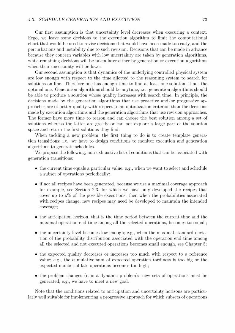
4.3. SCHEDULE GENERATION AND EXECUTION 73
Our first assumption is that uncertainty level decreases when executing a context.Ergo, we leave some decisions to the execution algorithm to limit the computationaleffort that would be used to revise decisions that would have been made too early, and theperturbations and instability due to such revision. Decisions that can be made in advancebecause they concern variables with low uncertainty are taken by generation algorithms,while remaining decisions will be taken later either by generation or execution algorithmswhen their uncertainty will be lower.
Our second assumption is that dynamics of the underlying controlled physical systemare low enough with respect to the time allotted to the reasoning system to search forsolutions on line. Therefore one has enough time to find at least one solution, if not theoptimal one. Generation algorithms should be anytime; i.e., generation algorithms shouldbe able to produce a solution whose quality increases with search time. In principle, thedecisions made by the generation algorithms that use proactive and/or progressive ap-proaches are of better quality with respect to an optimization criterion than the decisionsmade by execution algorithms and the generation algorithms that use revision approaches.The former have more time to reason and can choose the best solution among a set ofsolutions whereas the latter are greedy or can not explore a large part of the solutionspace and return the first solutions they find.
When tackling a new problem, the first thing to do is to create template genera-tion transitions; i.e., we have to design conditions to monitor execution and generationalgorithms to generate schedules.
We propose the following, non-exhaustive list of conditions that can be associated withgeneration transitions:
• the current time equals a particular value; e.g., when we want to select and schedulea subset of operations periodically;
• if not all recipes have been generated, because we use a maximal coverage approachfor example, see Section 2.3, for which we have only developed the recipes thatcover up to x% of the possible executions, then when the probabilities associatedwith recipes change, new recipes may need be developed to maintain the intendedcoverage;
• the anticipation horizon, that is the time period between the current time and themaximal operation end time among all the selected operations, becomes too small;
• the uncertainty level becomes low enough; e.g., when the maximal standard devia-tion of the probability distribution associated with the operation end time amongall the selected and not executed operations becomes small enough, see Chapter 5;
• the expected quality decreases or increases too much with respect to a referencevalue; e.g., the cumulative sum of expected operation tardiness is too big or theexpected number of late operations becomes too high;
• the problem changes (it is a dynamic problem): new sets of operations must begenerated; e.g., we have to meet a new goal.
Note that the conditions related to anticipation and uncertainty horizons are particu-larly well suitable for implementing a progressive approach for which subsets of operations

74 CHAPTER 4. THEORETICAL MODEL
are incrementally selected and scheduled. There is also no limitation to implementing aproactive technique since it depends on how distributions are used and what optimiza-tion criteria are used by the generation algorithms to select robust solutions; e.g., it ispossible to use a deterministic approximation of the problem and use simulation to filtersolutions when dealing with probabilistic problems, see Chapter 5 for example. Note alsothat the last item of condition can be associated with generation transitions that revisethe partial or complete schedule included in the current context by changing decisions.Any constraint of our model that is violated during execution has to be associated witha generation transition that changes the already made decisions if we want an adaptivegeneration-execution system; e.g., a machine breaks down or the memory for storing datais almost full.
It is also important to endow the automaton model with a procedure that updates dis-tributions during execution periodically and when events occur, because some conditionsmay only be met once distributions are updated.
One of the generation algorithms should be designed to select a subset of operationsthat are used to reason and make decisions. The selection can take into account thetime horizon, the uncertainty level, and the probabilities associated with the mutuallyexclusive recipes.
When the selection is done with respect to the time horizon, we mean that the selec-tion of operations starts when the anticipation horizon becomes too small and stops whenthe time period between the current time and the ends/starts of the selected operationsis long enough. When selecting operations with respect to uncertainty level that signifiesthat we select the operations whose uncertainty level is not too high with respect to athreshold; e.g., an operation is selected if the standard deviation of the probability distri-bution associated with its end time is not too high with respect to a threshold. However,we cannot delay an operation again and again because there is too much uncertaintyassociated with its execution, otherwise the quality decreases. We thus have to take intoaccount both quality and uncertainty level when selecting operations.
In case there are mutually exclusive recipes and a maximal coverage approach has beenadopted, the selection takes into account the associated probabilities; i.e., the operationsof a recipe are selected if their probabilities of being executed are high enough with respectto the maximal coverage threshold.
This selection procedure can limit the space and time complexities of the sub-problemto solve because the size of its search space is limited. This is an important property sincesearch time and memory can be limited in a number of application domains; for instance,when such a decision-making system is implemented on board of an autonomous system,such as a satellite.
Our automaton model comprises only one execution context at any time. In case ageneration transition is fired, a new execution context is generated and the old contextis removed from the automaton. This automaton develops dynamically and we do notknow a priori the number of execution contexts that are going to be generated duringexecution, what generation transitions are going to be fired, and the precise time instantsat which they are going to be fired during execution, apart from particular synchronousgeneration transitions that are fired at predicted precise time instants.
To summarize the behavior of our automaton model, we can remember that each con-text contains a partial flexible baseline schedule that an execution algorithm instantiates,and that a generation algorithm modifies or completes with respect to what effectively

4.4. A TOY EXAMPLE 75
happens during execution. Any general resolution approach that has been identified inChapter 2; i.e., a revision technique, a proactive technique, a progressive technique, or anycombination thereof can be implemented by instantiating such a model: there are gener-ation transitions that are responsible for revising schedules, other generation transitionsselect new sub-sets of operations to complete schedules, and a generation algorithm can bedesigned to produce more or less proactive schedules. Chapter 5 presents an instantiationof this automaton model for addressing scheduling problems with probabilistic processingtimes.
In the next section, we present a toy example that demonstrates how such an automa-ton model is instantiated when using a mixed approach.
4.4 A Toy ExampleThis section presents a toy example that shows how our generation-execution model isapplied in practice. The following toy example is inspired by our application domain, seeSection 3.2.
We assume we have to perform a set of tasks:
• construction of three roads road1, road2, and road3;
• construction of two houses house1 and house2;
• digging of a tunnel in one of two alternative ways tunnel1 and tunnel2 dependingon geological conditions observed at the end of road1;
• preparation of dam foundations foundation.
In addition, we assume we can use two trucks and each task requires one of them excepthouse1 that requires both. There are precedence relations between tasks, due dates, anda tardiness-cost function. Task durations are imprecise and modeled by probability dis-tributions. Our objective is to generate a schedule that minimizes the expected tardinesscost.
Figure 4.3 represents the temporal constraints between tasks of this small dam-con-struction project. This is a directed AND/OR graph. Each box symbolizes a task andthe box lengths depend on task durations. Arcs represent precedence constraints betweentasks; e.g., road2 must start after the end of road1. Conjunctions are represented by arcsconnected with small arcs of a circle; e.g., tasks house2 and road2 might be executed inany order or in parallel. Disjunctions are represented by arcs that are not connected witharcs of a circle; e.g., tasks tunnel1 and tunnel2 are mutually exclusive. Each recipe isassociated with a probability of being executed that may vary during execution.
When creating a generation-execution model for this toy problem, the first phaseconsists in deciding whether we want to monitor schedule execution. Since our knowledgeabout uncertainty is limited to probability distributions, we want to be able to changedecisions when expected tardiness cost deviates too much from its baseline value. Inaddition, we want to be able to make decisions on a gliding-time horizon to limit ourcommitment. For these reasons, we need to monitor schedule execution. We decide todesign two template generation transitions. The revision generation transition is activeduring execution, whereas the progression generation transition is active as long as there

76 CHAPTER 4. THEORETICAL MODEL
house1 house2
road2road1 road3
tunnel1
tunnel2
foundation
Figure 4.3: Temporal representation of a small dam-construction project.
is at least one task that is still not scheduled. We decide to use the same executionalgorithm for any execution context. This execution algorithm fixes task start times asearly as possible.
The first execution context ect1 is generated off line since we need to schedule atleast one task before starting execution. Figure 4.4 represents ect1. Notice that ect1 onlyincludes a subset of tasks since our progression generation algorithm makes schedulingdecisions on a short-term horizon. tunnel1 is scheduled because its probability of beingexecuted is higher than the one associated with tunnel2 at this time. In addition, twoadditional precedence constraints are included in ect1 as we cannot use more than twotrucks at the same time: road2 starts after the end of house1; house2 starts after the endof road2 . These sequencing decisions are made to minimize the expected tardiness costgiven probability distributions.
We start executing ect1. During the execution of road1, the probability associated withtunnel1 decreases, so the probability associated with tunnel2 increases. These changesactivate the progression generation transition and a new context ect2 is generated. Fig-ure 4.5 represents ect2 that includes both tunnel1 and tunnel2.
When road1 finishes, we observe geological conditions and choose tunnel2 accordingly.Figure 4.6 represents ect2 at this time. Note that the branching node disappears in ect2.
The execution of ect2 continues until we observe that the mean end time of house1 islater than predicted in such a way that house2 is postponed and the expected tardinesscost increases too much with respect to its baseline value. This activates the revisiongeneration transition that creates a new context ect3. Figure 4.7 represents ect3, whereroad2 is now sequenced after house2.
We are now executing ect3. When house2 is executing, the progression generationtransition is activated since we need to select and schedule new tasks to maintain the leadof generation over execution. A new context ect4, which includes all tasks, is generated,see Figure 4.8. Notice that the template progression generation transition is no longeractive as all tasks have now been scheduled.
We do not develop this example model further since the rest would not illustrate other

4.4. A TOY EXAMPLE 77
house1 house2
road2road1
tunnel1
ect1
gtrprogression
gtrrevision
Figure 4.4: Execution context generated before starting execution.
house1 house2
road2
tunnel2
road1
tunnel1
ect2
gtrprogression
gtrrevision
Figure 4.5: Execution context generated during the execution of road1.

78 CHAPTER 4. THEORETICAL MODEL
house1 house2
road2
tunnel2
road1
ect2
gtrprogression
gtrrevision
Figure 4.6: Execution context generated when road1 ends.
road2
house2
road1
tunnel2
house1
ect3
gtrprogression
gtrrevision
Figure 4.7: Execution context generated during the execution of house1.

4.5. SUMMARY AND GENERAL COMMENTS 79
road2road1
house1
road3
house2
tunnel2
foundation
gtrrevision
ect4
Figure 4.8: Execution context generated during the execution of house2.
characteristics of our generation-execution model.
4.5 Summary and General Comments
In this chapter, we presented our theoretical generation-execution model. In the firstsection, we informally described how expressive this model is. In the second section, wegave definitions that are necessary to define our model. In the third section, we describedhow generation and execution are interleaved with our model. In the fourth section,we illustrated our model with a toy example inspired by our application domain. Thisexample demonstrates how our model can be instantiated to mix revision, proactive, andprogressive generation-execution techniques.
Of course, this model is not completely described; for instance, all types of constraintsare not made explicit. More than that, we have intentionally left apart optimizationconcerns: what types of optimization criteria could be modeled, and what would bethe properties of our model with respect to stability and robustness issues for instance?Actually, our model is only a representation model that does not address reasoning issues;i.e., what there really is within generation and execution algorithms, our intention wasindeed merely to show how and where proactive, revision, and progressive techniquesshould appear and interact with each other in a system that would interleave generationand execution of a schedule, which we have tried to design as generic as possible.
This model is open and could be extended in different directions. For example, wecould develop generation algorithms that can deal with causal relationships.
The combinatorial problems that can be solved by using this model can be composedof causal relationships between its data. These causal relationships can be expressed withconditional probability distributions, such as in a Bayesian network, see Section 1.3.3; e.g.,the processing time or the distribution of the processing time of an operation o1 dependson the outside humidity when we start executing o1 and we do not know in advancethe outside humidity with accuracy. There may be conditional probability distributions

80 CHAPTER 4. THEORETICAL MODEL
depending on time as well.A set of mutually exclusive recipes can be seen as a sub-goal that is reached when one
of its mutually exclusive recipes is chosen to be executed from the task-planning pointof view. Thus, the problem we can tackle with this model lies somewhere in betweentask planning and scheduling since it comprises mutually exclusive recipes. A future workwould consist in extending the definition of the problem with sub-goals. A thought aboutthe rules to insert operations or recipes into the schedule and to remove operations orrecipes from the schedule would be useful. The definitions of an operation and a recipewould be also extended by introducing preconditions and effects.
In other words, to design this model, we have been inspired by task planning and inparticular, conditional task planning, see Section 1.3.5. However, this model is used inthe context of scheduling. We could really bridge the gap between scheduling and taskplanning by integrating more aspects of task planning in this model.
The next chapter describes our experimental system, the scheduling problems un-der uncertainty we have tackled by implementing instantiations of the theoretical modelpresented in this chapter, and some commented results.

Chapter 5
Experimental System
In Chapter 2, we presented a review of planning and scheduling under uncertainty andit was noted there are currently few scheduling systems that can tackle complex prob-
lems under uncertainty with mixed approaches. We are thus motivated to design andimplement a scheduling system in which combined solving techniques are applied off lineand on line to solve large-scale scheduling problems with uncertainty. In this chapter,we propose such a system that is actually an instantiation of the theoretical automatonmodel presented in Chapter 4.
The first section of this chapter presents the scheduling problem we tackle. The secondsection we detail the architecture of our prototype, the resolution techniques implemented,how it interleaves generation and execution, and its parameters and indicators. Thethird section describes the revision-proactive approach that is integrated in our prototypeand an experimental study. The fourth section is dedicated to the progressive-proactivetechnique that is implemented in our prototype. The fifth section discusses general aspectsof our experimental system and the last section summarizes the chapter.
5.1 Scheduling Problem
We are interested in scheduling problems with probabilistic operation durations; i.e., op-eration end times are observed during execution. Moreover, resources may break down:for each resource, the duration between two consecutive breakdowns is probabilistic andbreakdown durations are also probabilistic. In addition, there are alternative unary re-sources; i.e., an operation can require one of a number of resources. In other words, weaddress job-shop problems with general allocation, probabilistic operation durations anduncertain resources.
The problem is a randomly generated n × m scheduling problem and consists in nprocess plans. Each process plan pi consists in a sequence of m operations (oij). For eachoperation, a given number k of randomly picked alternative resources constitute the setof possible resources. There are n ×m operations to be processed and the total numberof resources is equal to q. A process plan is thus defined as a job whose each operationwill be executed on one of k alternative resources.
We assume operations are not preemptive.
81

82 CHAPTER 5. EXPERIMENTAL SYSTEM
5.1.1 Costs
This scheduling problem is an optimization problem where the objective is to find theschedule that minimizes the average global cost. We distinguish two types of schedulecosts: tardiness and allocation costs.
Tardiness Cost
Each process plan pi ∈ P is associated with a due date duei. If the last executed operationof pi finishes later than duei, then a cost tardiCosteffi = tardieffi × φi is incurred, calledtardiness cost. tardieffi depends on how late pi finishes: tardieffi = max(endpeff
i − duei, 0),where endpeff
i is the effective end time of pi, observed during execution. If pi finishesearlier than or at duei, then tardieffi is equal to zero. Tardiness costs increase linearlywith respect to how late process plans finish: a weight, φi, is applied to each time unitafter the due date that the process plan has not yet finished. A schedule is associatedwith a tardiness cost Ktardiness defined as follows.
Ktardiness =∑
∀pi∈P
tardiCosteffi
Allocation Cost
Another cost, called allocation cost, is associated with each resource allocation: whena given operation oij ∈ O is executed with a given resource rl ∈ Rij, it incurs a costallocCostijl. Note that allocCostijl is not completely random since it depends on resourcerl and there are more or less cheap resources. A schedule is defined by a set of allocationsand associated with an allocation cost Kallocation: each operation oij is effectively allocatedto a resource reff ∈ Rij and this allocation costs allocCosteffij .
Kallocation =∑
∀oij∈O
allocCosteffij
Global Cost
The global cost K represents the whole cost of a solution; this cost takes both allocationand tardiness costs into account. It is formally defined as:
K = Kallocation + Ktardiness
Each scheduling problem is characterized by a maximal global cost, Kmax, that definesan upper bound with respect to the schedule costs. We want to maximize the probabilitythat the global cost is less than the maximal global cost; this can be formally expressedas follows.
max Pr(K ≤ Kmax)
Note that tardiness and allocation costs are antagonistic since the tardiness cost islikely to be high if we only want to reduce allocation cost by choosing systematically thecheapest resources when allocating operations, and conversely the allocation cost is likelyto be high if we only take tardiness cost into account since this increases the likelihoodthat more expensive resources will be made so that operations can be done in parallel.

5.2. ARCHITECTURE 83
met?
condition
progress.
selectionof a sub-problem
met?
condition
revision
solver
worldsimulator
controller
decisionsobservations
flexible
scheduledecisions
observationsyes
no
model
problem
non-deterministic
complete
yes
no
Figure 5.1: The general schema of our software prototype.
5.2 Architecture
In Figure 5.1, our general schedule generation-execution schema is represented. It is com-posed of different modules: a solver, a controller, and a world simulator. The solvermodule is in charge of solving a problem and sends the solution to the controller module.The controller module is responsible for adapting the solution it receives from the solvermodule with respect to what happens during execution, in particular, it monitors con-ditions and calls the solver module when these conditions are met. The world simulatorsimulates a non-deterministic execution environment.
5.2.1 Solver
The solver module is in charge of producing a flexible schedule. It has to solve a sub-problem modeled by a constraint network whose a subset of variables are associated withknown probability distributions and another subset of non-controllable variables whoseprobability distributions are unknown. The resolution process of the solver module is de-picted in Figure 5.2. First, the user models a non-deterministic problem with variables andconditions. This model is connected to the different modules of the software prototype.Then, the resolution procedure proceeds as follows: (1) a deterministic approximationconstraint model is generated from the non-deterministic sub-problem model, the searchspace of this combinatorial problem is then partially explored and the best flexible solution

84 CHAPTER 5. EXPERIMENTAL SYSTEM
model
sub-problem
non-deterministic generationof a deterministic
approximationconstraint
solver
flexiblesolution
Monte-Carlosimulations
flexible solutionstored if best
time limit
exceeded?
solution sentto controller
best flexible
distributions
probability
yes
no
Figure 5.2: The solver module of our resolution prototype.
is returned (operation start times are not set); (2) we run a number of simulations basedon the partial-order solution and the known probabilistic distributions of the underlyingsub-problem; (3) if the simulated flexible solution is better than the best solution foundso far in terms of optimization characteristics (standard deviation and mean), then it isstored and we start a new search. We iterate the resolution procedure until the allottedtime for searching is elapsed. When we stop the resolution procedure the best flexibleschedule is sent to the controller module. Note that the generation of a deterministicapproximation and the Monte-Carlo simulator are parametrized. It is possible to unplugsimulation as well.
The solver module is called initially to compute the first execution context and duringexecution when some conditions are met. These conditions are monitored during executionby the controller module, see algorithm β presented in Chapter 4.
5.2.2 Controller
The controller module makes the remaining decisions; i.e., these are the decisions thathave not been made by the solver module. The controller module makes these decisionswith respect to problem constraints, observations, and a scheduling policy; e.g., executeoperations as soon as possible is a standard scheduling policy. The controller module isalso responsible for monitoring schedule execution and calling reactively the solver modulewhen progressive or revision conditions are met. The controller module plays a third role:since these conditions are expressed with non-controllable variables (e.g., operation end

5.2. ARCHITECTURE 85
times), we have to estimate the current characteristics (means and standard deviations)associated with these non-controllable variables. The controller has its own simulator andwe can update the means and standard deviations by running simulations periodicallyand/or when an unexpected event occurs.
A constraint-based resolution combined with an execution controller are also used bythe scheduling system proposed by Cesta and Rasconi [39]. This system is capable ofreactively maintaining the consistency of the schedule in spite of possible unexpectedevents that occur at schedule execution time. A new solution, computed after an unex-pected event occurs, must be as close as possible to the preceding solution to maximizethe level of continuity that is the stability. However, their current system does not permita schedule generation on a gliding time horizon.
Progression and Revision Conditions
When progression conditions are met, we have to select and schedule a new subset ofoperations to anticipate execution; e.g., when the time period between the current timeand the end time of the last scheduled operation is too short, we need to select a newset of operations. This permits a progressive decision-making since the complete schedul-ing problem is split into sub-problems and solved piece by piece during execution withuncertainty level decreasing.
We have to change scheduling decisions; i.e., we have to revise the current schedulewhen revision conditions are met: the current schedule is not any longer executable orits expected quality deviates too much with respect to its baseline quality computed justafter its generation by the solver module. For example, we reschedule when a resourcebreaks down.
The generation-execution loop is controlled by the controller on the basis of theseconditions.
5.2.3 World Simulator
The world simulator module generates unexpected events it sends to the controller module;i.e., it sends operation end times, and breakdown start and end times. The probabilitydistributions used to generate these unexpected events can be different from those knownby the controller and the solver modules.
5.2.4 Resolution Techniques
In this section, we present different components that can be combined to tackle thescheduling problem presented in the preceding section.
Constraint-based Search
This component belongs to the solver module. The role of this component is to find aflexible solution of the constraint-based scheduling problem model that aims at minimizingthe expected global cost Kexp. Kexp is computed by running Monte-Carlo simulation. Thesolution returned by the solver module is continuously flexible since only operation starttimes are not decided.

86 CHAPTER 5. EXPERIMENTAL SYSTEM
The search space is divided into two parts: the allocation part and the sequencingpart. In the allocation part, allocation decisions are made and in the sequencing part, foreach unary resource, we order the operations requiring it.
We experimented with several heuristics to generate problem instances. The mainissue when generating these problem instances is to find maximal global costs that areneither too high nor too low with respect to the other problem instance characteristics.This is particularly difficult since the cost constraints are rather loose, so they do notpropagate efficiently.
During search, allocation decisions are made first and we have to proceed in two stepsas follows until all operations are allocated: we choose an operation oij and then we decidewhat resource rl to allocate to oij.
The operation that we allocate first is randomly chosen as follows. We associate aprobability to each operation oij that depends on a parameter ω and the dispersion of itsallocation costs. The higher ω, the more random the choice. The higher its local disper-sion, the higher its probability. The local dispersion dispij of operation oij is computedas follows:
dispij =1∑
∀rl∈Rij
1ε+allocCostijl+min∀rk∈Rij
(allocCostijk)
,
where ε → 0. The main idea when using the dispersion of the allocation costs is tochoose the operations to allocate depending on the numbers of their possible alternativeresources that have a good chance of being reduced by propagating the cost constraints ifthey are later allocated. The better the chance of being reduced, the highest the priorityof allocating the operation.
The allocation decisions are randomly made as follows. We associate a discrete prob-ability distribution with the range of possible allocations such that the probability ofallocating operation oij to resource rl decreases with the corresponding allocation costallocCostijl: the higher the allocation cost, the lower the probability. The randomness ofthe distribution depends on ω: the higher ω, the more random the choice of the resource.
These allocation heuristics are effective since (i) they avoid always making the sameallocation decisions and (ii) making allocation decisions is not completely random. More-over, ω controls the randomness of the decision-making.
Sequencing decisions are then chronologically1 made by using the following heuristic:for each resource, we order first the operation with the minimal earliest start time, tiesare broken by ranking first the operation that belongs to the most tardy process plan orthat belongs to the process plan whose end is the closest to its due date.
We have experimented two meta-heuristics, that is, fast random restart, and LargeNeighborhood Search (LNS), using alternatively two search techniques Depth-First Search(DFS) and Slice-Based Search (SBS) as components.
DFS consists in visiting first the child node by following the heuristic choice andchronologically backtracking. This is a constructive search and it is not effective in ourcase since our search tree is divided into allocation nodes and sequencing nodes and wewant to change about the same number of allocation decisions as the number of changedsequencing decisions.
SBS is close to Limited Discrepancy Search (LDS) [81]. LDS consists in exploring
1Here “chronologically” means that we do not systematically sequence all operations allocated to aresource before sequencing the operations allocated to another resource.

5.2. ARCHITECTURE 87
nodes based on how many decisions have been made so far against the decisions thatthe heuristic would make. In search trees, right moves are considered mistakes (they donot follow heuristic decisions) and left moves are considered correct decisions (decisionsadvised by heuristics). LDS first looks in the paths of the tree with fewer right moves. Aright move in the path from the root node of the search tree to the current node is knownas a discrepancy. LDS is parametrized such that it will first look at paths with 0 or 1discrepancy, then the paths with 2 discrepancies, then the paths with 3 discrepancies andso on. The maximal number of discrepancies of a path explored by LDS for a sub-problemis limited. LDS is a constructive search that is more efficient than DFS for solving ourproblem instances since we can change allocation decisions more often when using LDS.The reader can read a paper by Beck and Perron that details SBS [19].
Fast random restart consists in probing the search tree several times each time makingdifferent decisions since heuristics for making allocation decisions are randomized [77].Fast random restart is a constructive search but it is not complete. As each probe consistsin a search with few backtracks we quickly restart search from scratch.
LNS starts from a solution and tries to improve it iteratively by changing a subset ofdecisions. It consists in relaxing a subset of decisions; i.e., these decision variables are de-instantiated. Then, we iteratively explore a limited search space with the rest of decisionsfrozen. This technique fits well large-scale combinatorial problems since it permits theexploration of different search subspaces.
The best combination of search techniques we have experimented when generatingproblem instances is the following. Fast random restarts are first performed for findinga good solution given a time limit. Then we use LNS with DFS to improve iterativelythe solution quality given another time limit. These search techniques are used becausewe want to solve complex and large scheduling problems; i.e., we want to solve probleminstances with up to 5,000 operations, and fast random restart and LNS are anytimesearch algorithms. The two moves for LNS that perform best are the following. The firstone relaxes a subset of process plans that are randomly chosen. A process plan is relaxedby removing allocation and sequencing decisions related to its operations. The secondone relaxes a subset of operations that are randomly picked. An operation is relaxed byremoving its sequencing and allocation decisions. These two moves are interleaved forexploring different search subspaces. LNS with DFS is efficient because it does not tacklethe complete problem but sub-problems that are randomly selected. Sub-problems areeasier to solve than the complete problem and the search space is randomly explored, sowe can easily escape from local optima.
Monte-Carlo Simulation
For updating unknown probability distributions associated with non-controllable variablessuch as operation end times, we use Monte-Carlo simulation. A Monte-Carlo simulationrun consists in randomly picking a value for each random variable such that the two setsof values that are randomly picked for two consecutive simulation runs may be completelydifferent. Our application domain implies computations that are complex and difficult,indeed impossible to do with analytical approaches. Moreover, our application domaindoes not require exact computations since it is not critical; i.e., the impact of our decisionsis not too serious with respect to the underlying physical system. A spacecraft is a criticalsystem since it can break down or crash after taking a bad decision and it is difficult to

88 CHAPTER 5. EXPERIMENTAL SYSTEM
0 10 20 30 40 50 60 700
0.01
0.02
0.03
0.04
0.05
0.06
0.07
0.08
0.09
0.1
0.11
0.12
Figure 5.3: Two truncated and normalized normal laws.
repair it: its mission failed. However, a manufacturing workshop is a less critical systemsince we can usually repair it when making a bad decision. For computing expectedoperation end times, we run a series of simulations on the flexible schedule at handby assuming operations are executed as soon as possible. For each operation oij that isallocated and sequenced but not yet executed, we randomly pick a set of possible durationsand for each resource that is allocated to oij, we randomly pick a series of breakdowns.For generating resource breakdowns, we proceed as follows: for each resource allocated tooij, the last breakdown generated occurs after the end time of oij; if a breakdown overlapswith the operation, then the operation end time is delayed.
For running simulation, we use a precedence graph that is generated for the constraintnetwork: each node represents an operation and each arc represents a precedence con-straint between two operations. We then topologically sort the precedence graph and usethis ordering in the simulations. The simulation horizon equals the sum of all operationdurations. The complexity of a single simulation run is in O(nbBk + nbOp + nbPCt),where nbBk is the number of resource breakdowns, nbOp is the number of operationsand nbPCt is the number of precedence constraints; it is in O(nbBk + nbOp) for ourproblem since there are fewer unary resources than operations and our problem has thesame number of precedence constraints as a job-shop scheduling problem.
Note that the number of simulation runs and the confidence intervals associated withunknown probability distributions are related: the width of each confidence interval is afunction of 1/
√nbSimRuns, where nbSimRuns is the number of simulation runs.

5.2. ARCHITECTURE 89
Controller
The implemented controller is in charge of updating both known and unknown probabilitydistributions.
The probability distributions we know, such as the probability distributions associ-ated with resource breakdown start times, resource breakdown durations, and operationdurations, are truncated and normalized. Suppose we have an operation whose executionstarted at date t = 0 and whose duration, which is between 10 and 60, follows a nor-mal law of mean 30 and standard deviation 10. This operation duration is depicted bythe dotted curve in Figure 5.3. Now suppose that at date t = 35 the operation is stillexecuting, we will assume that the probability distribution of the operation end time isthe initial law truncated on the interval [35, 60] and renormalized as shown by the solidcurve in Figure 5.3. More formally, if the initial probability law of an operation durationis described by a distribution function p0(dur) defined in [durmin, durmax], and if the op-eration has been executed since dur0 units of time, the current distribution is defined bythe probability distribution pdur0(dur) as follows:
∀dur ∈ [dur0, durmax], pdur0(dur) =p0(dur)∫ durmax
dur0 p0(t)dt.
The probability distributions to be computed are updated by running Monte-Carlosimulation, see Section 5.2.4.
5.2.5 Experimental Parameters and Indicators
This section describes how we proceed to compare experimentally different approaches tosolve a scheduling problem with uncertain operation durations, machine breakdowns, andalternative resources. We can fix different parameters and assess solutions with indicators.Parameters are independent of each other.
Problem Instance Generation
Concerning the scheduling problem, we can experiment with the following parameters:
• the number of process plans;
• the number of resources;
• the number of operations per process plan;
• the number of alternative resources per operation;
• the due dates;
• the uncertainty level associated with operation durations;
• the uncertainty level associated with durations between two consecutive machinebreakdowns;
• the uncertainty level associated with machine breakdown durations.
In addition, it is possible to make the scheduling problem more or less tight by choosingthe number of resources and the due dates.

90 CHAPTER 5. EXPERIMENTAL SYSTEM
Search
Constraint-based search consists in different parameters such as the maximal number offails and the time limit. Different search techniques can be compared such as local search,LDS, DFS, etc., see Section 5.2.4. There are also parameters that characterize particularsearch techniques such as LNS for which we can implement and test different moves.
Revision, Progressive, and Proactive Techniques
A revision technique is parametrized by choosing a revision criterion and a sensitivityfactor (ς). A revision criterion is a condition that is monitored during execution; e.g., wemonitor the absolute difference between the expected quality, computed before execution,and the current expected quality, computed during execution based on what we observe,and we compare this absolute difference with a reference value. If it is met, then wereschedule. A sensitivity factor sets the sensitivity of the revision criterion with respectto perturbations that occur during execution. The sensitivity factor is set to indirectlychoose the search effort that depends on the number of reschedulings that occur duringexecution.
A progressive technique is characterized by four parameters that can be set to chooseindirectly the anticipation horizon and the size of each sub-problem: δtmin controls theanticipation horizon with respect to time, σtmin controls the anticipation horizon withrespect to the uncertainty level, δtmax controls the size of each sub-problem with respectto time (reasoning and commitment horizon), and σtmax controls the size of each sub-problem with respect to the uncertainty level. These four parameters are expressed withrespect to uncertainty level and temporal horizon.
A proactive technique is set by two main parameters. The first parameter proactgene isused to generate the deterministic sub-problem model from the non-deterministic problemmodel; i.e., we choose a value for each random variable: operation durations, and resourcebreakdown start times and durations. A possibility is to choose and use the average valuesof distributions. The greater the values chosen, the more proactive the technique. Thesecond parameter proactsimu is Boolean and determines whether Monte-Carlo simulationis used or not to find flexible solutions. Moreover, the number of simulation runs canbe chosen. Beck and Wilson studied proactive techniques to solve probabilistic job-shopproblems [21].
Indicators
There exist a number of possible indicators to assess a schedule or a scheduling system:
• the intrinsic quality of a solution that is the absolute quality;
• the robustness of solution quality that is the relative quality (how quality changeswith respect to its initial value);
• the stability of decisions (relative indicator) that is how many decisions are changedwith respect to initial commitments;
• the search effort measured with CPU time spent for searching solutions and thenumber of reschedulings that occur;

5.3. REVISION-PROACTIVE APPROACH 91
• memory consumption.
Note that we have not yet implemented stability indicators but it would be possibleto extend the prototype in this way.
5.3 Revision-Proactive ApproachIn this section, we present a mixed technique that has been implemented in our softwareprototype. It combines a revision approach with a proactive approach.
5.3.1 Revision Approach
The revision approach consists in monitoring a condition called the revision criterionduring execution and when the condition is met we change decisions; i.e., we reschedulewhen the revision condition is met. This is a generation-execution loop. The revisioncriterion depends on uncontrollable variables such as operation end times. The revisioncriterion depends on a sensitivity factor ς that controls indirectly the search effort; i.e.,the number of reschedulings during execution depends on ς. ς fixes how much the effectiveor expected values can deviate from nominal ones, such that nominal values are updatedeach time we (re)schedule. Rescheduling is done by using constraint-based search, seeSection 5.2.4, combined possibly with Monte-Carlo simulation, see Section 5.2.4.
The initial (off-line) schedule starts execution and we must decide when to reschedule.The main idea behind the parameters investigated here is that we use simulation to de-termine when to reschedule. We start execution using the baseline schedule and a simpleexecution policy: operations are started as soon as possible given the precedence con-straints in the original problem, the operation sequences defined by the baseline schedule,and the effective operation durations that are observed. During execution of the sched-ule, we choose to evaluate the need for rescheduling whenever an operation ends. Thefirst step consists then in updating the truncated probability distributions representingour view of the uncertain variables, as discussed in Section 5.3.3. The second step is tocalculate a chosen revision criterion that depends on expected values of some variables inthe problem. If the difference is too large between the expected values and the nominalvalues, then it means that the assumptions made during the schedule computation arebecoming less and less relevant thus there is a chance that rescheduling will improve thecurrent schedule.
The expected values for the variables we are interested in are estimated through theuse of Monte-Carlo simulation. According to the currently executing schedule and thecurrent probability distributions, we run 1,000 simulations whenever an operation ends.Each simulation run allows one to calculate the values of the variables we are monitoringand by running simulations we can calculate approximately their means and standarddeviations. The expected value of the variable is its mean value obtained after simulating.If we decide to reschedule, the current schedule is ignored and a new schedule is generatedexcept for the operations that have already started or finished executing. Each schedulingproblem is represented by a constraint network whose constraints must be satisfied bysolutions. We here deal with Dynamic Constraint-Satisfaction Problems, see Section 1.3.3,since each time we reschedule it amounts to redefining a new sub-problem by changingthe previous approximated deterministic problem model that has been solved to find

92 CHAPTER 5. EXPERIMENTAL SYSTEM
the current baseline schedule. The previous approximated problem model is changedby taking into account what has been observed since the last rescheduling. We use thecurrent distributions of the operation end times and resource breakdown end times; asubset of the current distributions are truncated.
5.3.2 Proactive Approach
The proactive approach consists in finding flexible schedules that minimize the averageglobal cost using knowledge about uncertain data. This search process can be run whenusing the solver module. The first way of making a solution more robust in our system isto approximate the deterministic constraint-based problem model by taking into accountuncertainty; e.g., operation durations of the deterministic problem model are chosen tocover 50% or more of possible operation durations. The second way of finding robustsolutions is to use Monte-Carlo simulation during search. Beck and Wilson experimentedsuch an approach for solving job-shop scheduling problems with probabilistic durationswhere expected makespan is minimized [20, 21]. When using simulation, they modelthe problem with a constraint network in which operation durations are chosen equalto or greater than the mean operation durations. The constraint model is solved by abranch-and-bound procedure with constraint propagation. Each flexible solution (oper-ation start times are not set in time) is simulated for computing an estimation of thecorresponding expected makespan. During simulation, we start operations as soon aspossible. Simulations can also be run and expected values computed to prune the searchtree at intermediary nodes; i.e., when only a subset of decisions are made but it is toocostly to be applied for solving large scale decision problems.
5.3.3 Experimental Studies
This section reports results obtained by experimenting a proactive-revision techniquebased on constraint programming and simulation for schedule execution monitoring andon-line rescheduling. We tackle job-shop scheduling problems with probabilistic operationdurations. This is a subset of the scheduling problems that were described in Section 5.1.Some model features are disabled: there are no alternative resources and no allocationcosts.
Problem Description
Our experiments concern the job-shop scheduling problem (JSSP) with probabilistic oper-ation durations and makespan minimization. In this section, we present our assumptionsabout the evolution of the uncertainty of operation durations during execution.
Each uncertain operation duration is modeled by a variable that follows a probabilitydistribution and is associated with a domain. Any probability law can be used (normal,uniform, etc.), however, as an operation duration must be strictly positive, the lawsare truncated. At execution, we know the effective duration of an operation only whenthe operation ends and we learn this piece of information from the environment (worldsimulator). The only decision is when to start the execution of each operation. As aconsequence, we know at each moment, during the execution which are the operationsthat have been executed, the ones that are currently executing, and the ones that have

5.3. REVISION-PROACTIVE APPROACH 93
not been started yet. When an operation is still executing and its minimum possibleduration has been exceeded, our information on the uncertainty can be updated since theset of possible durations is now reduced. Therefore, the probability distribution is furthertruncated and renormalized, see Section 5.2.4. We update data at specific points in timethat are the moments when we want to decide if we reschedule or not, and hence we needto know the precise current state.
The effective duration of an operation is the duration that is observed during execution,see Definition 1.3.1. An execution scenario is a set of all effective operation durations.
A baseline schedule is a schedule where the operations on each resource are totally or-dered. The first baseline schedule is calculated off-line by solving a deterministic problemwhere operation durations equal the mean operation durations of the non-deterministicproblem. A Depth-First Search is used to explore the search space. During execution, anew baseline schedule is constructed if we decide to reschedule; in that case, this new base-line schedule is calculated by using both the effective durations of the operations alreadyexecuted and the mean durations of the other operations. Note that given our tuningof proactgene, one of the proactive parameters, a baseline schedule is proactive at a lowlevel since it is generated by using mean operation durations; i.e., only 50% of executionscenarios are covered locally when using mean operation durations. We do not know thepercentage of execution scenarios that are covered from a global point of view; i.e., whenwe consider the complete problem with temporal relations between operations. However,if Monte-Carlo simulation is used, the search technique can be much more proactive.
Experimental Results and Conclusions
In this section, we report the results of two experimental studies aiming at determiningthe impacts of the revision criterion and the uncertainty level on makespan with a limitedcomputational effort. All the programs run to perform these tests have been written inC++, use ILOG Scheduler 5.3 [88] for scheduling, and have been compiled with MicrosoftVisual C++ 6. The results presented here have been obtained with using a dual processorPentium II Xeon 450MHz with 256MB.
Impact of Revision Criterion on Makespan We report a study of the impact ofrevision criterion on effective makespan in this section. We investigated three differentrevision criteria for deciding when to reschedule.2
First, we describe formally the three criteria. All these criteria depend on a strictlypositive parameter called the sensitivity factor ς that can tune the sensitivity of therevision criteria. When ς is very small, there will not be any rescheduling. The larger thesensitivity factor ς, the higher the number of reschedulings (and the smaller the stabilityof the schedule).
The first criterion revCrit1 consists in monitoring the makespan and is defined asfollows: we reschedule when
Mexp >Mind
ς,
where Mexp is the current expected makespan and Mind is the makespan of the currentbaseline schedule. This criterion will not result in rescheduling if the effective operation
2The work reported in this section was partially published [25].

94 CHAPTER 5. EXPERIMENTAL SYSTEM
durations are shorter than expected. In other words, it does not allow “opportunistic”rescheduling that would take advantage of unexpectedly short execution times.
A second variation revCrit2, based on the first, is opportunistic because it reschedulesbased on the absolute difference between the expected and baseline makespans. Wereschedule when
|Mexp −Mind| >D
ς,
where D is the mean of all operation durations of the initial problem.The two versions based on makespan monitoring are a priori rather crude: we mainly
take into account the observed durations of the operations of the critical paths. If theseoperations do not slip too much, then, as a consequence, the makespan will not slip toomuch either. It is possible however, that the expected makespan remains approximatelystable while the executions of the operations that do not belong to the critical paths aresuch that it is possible to find a much better solution by rescheduling. We thus propose athird variation of the approach revCrit3 that takes into account each operation duration.We reschedule when ∑
Onew|endexp − endind|nbNewOp
>D
ς,
where Onew is the set of nbNewOp operations that were executing the last time werescheduled, and endexp and endind are respectively the expected and baseline operationend times.
The problem instances with imprecise durations are generated from classical JSSPinstances. Each operation is associated with a normal probability distribution with mean,p, corresponding to the duration in the classical instance, and with standard deviation α×pwith α > 0. α characterizes the degree of uncertainty of the problem. The higher α, thelarger the standard deviation of each operation duration so the more uncertainty in thesystem. α is constant and equals 0.3 for each experiment done in this first study.
During schedule execution, whenever we are informed by the environment that anoperation ends, we update all our data structures, and simulate the continued executionof the schedule. The updating frequency is sufficiently low to permit 1,000 simulation runseach time. When the end of an operation is observed, there might be other concurrentoperations still executing for which distributions are updated. We are using simulationto calculate the revision criterion and then we reschedule only if the revision criterion ismet.
Scheduling and rescheduling are done using the constraint programming approach witha standard chronological backtracking algorithm and a time limit of one second. The newschedule is the best solution found within the time limit using a depth-first search. Twoheuristic rules are used to make sequencing decisions: first, we have to select the resourceand second, we have to select the resource constraint to rank first on this resource. Theresource r with the minimal global slack is selected with priority, and then the operationrequiring r, with the minimal latest start time is ranked first on r. The global slack ofa resource is the slack time of the operations that are allocated to it. The global slackis computed on the basis of the temporal window of each operation; i.e., this temporalwindow is the time period between its earliest start time and its latest end time. Duringsearch constraint, propagation is used to prune the search tree, in particular Edge-Finder,

5.3. REVISION-PROACTIVE APPROACH 95
Mea
n ef
fect
ive
mak
espa
n
0 5 10 15 20 25 30 35 40 45 50 55 60 65 70 75 80 85
Mean number of reschedulings
1,230
1,240
1,250
1,260
1,270
1,280
1,290
1,300
1,310
1,320
1,330
1,340
1,350
criterion with makespancriterion with absolute makespancriterion with operation end timesmean off−line optimal makespan
Figure 5.4: Mean effective makespan for la11 with a low uncertainty.
see Section 1.2.4. Note that we do not use simulation to filter solutions found by the treesearch because we assume that a solution with a low deterministic makespan is also asolution with a low expected makespan [21].
The results shown on Figure 5.4 come from running 100 different execution scenariosper value of the sensitivity factor ς. These results are obtained from experimenting withthe problem la11 that consists of 100 operations. We observe that monitoring sched-ule execution with the use of each rescheduling criterion improves schedule quality; i.e.,mean effective makespan is smaller than the mean effective makespan obtained with-out rescheduling that equals 1,350: for example, after 2 reschedulings the mean effectivemakespan approximately equals 1,290 (4.4% of improvement). The most significant im-provement is obtained with less than about ten reschedulings. The mean off-line optimalmakespan equals the average of the 100 optimal makespans, each of them is computedoff line assuming we know the execution scenario in advance; i.e., we have to solve 100deterministic JSSPs to optimality. Each of these 100 optimal makespans is a lower boundon the best schedule quality that can be achieved. We actually experimented with otherliterature JSSPs of the same size: la12, la13, la14, abz5, abz6, orb1, orb2, orb3, andorb4. The results obtained with these instances corroborate these observations [99, 13, 9].These curves confirm the criterion based on the operation end times provides the smallestmakespan for a given computational effort since it is more opportunistic than the first tworevision criteria. We also think this is due to the fact that the operations placed close to

96 CHAPTER 5. EXPERIMENTAL SYSTEM
the start of the schedule have a smaller impact on makespan than the operations placedclose to the end of the schedule.
Impact of Uncertainty Level on Makespan In this section, we report a study thatinvestigates the impact of uncertainty level α on makespan. All experiments have beenrun with the same revision criterion. We chose the revision criterion revCrit3 presentedin the preceding paragraph; i.e., this is the revision criterion that takes into account alloperation durations. This revision criterion performs best when about ten reschedulingsare done.
Our study consists in varying the uncertainty level α and observe how the effectivemakespan changes accordingly. α directly changes the standard deviations of operationdurations: the higher α, the larger the standard deviations, that is, more imprecise oper-ation durations. We considered the same ten JSSP instances as those used in the study ofthe impact of the revision criterion on makespan, see the preceding section. We conductedthree series of experiments, each of them corresponds to a fixed value of α. The curvesrepresented on the next four figures have been obtained by testing 30 problem instances,100 different realizations per problem instance. The search procedure is the same as theone presented in the preceding section. The tree search is limited to one second whenrescheduling and we run 1,000 simulation runs each time an operation ends as well.
The curves on the next three figures represent the relationship between the meannumber of reschedulings and the mean relative error of effective makespan for thirtyproblem instances. We tested ten problem instances per uncertainty level. The meanrelative error of makespan is computed over the nbExecSce = 100 execution scenarios ofeach problem instance as follows.
mean relative error =1
nbExecSce×
nbExecSce∑sce=1
M effsce −Mopt
sce
Moptsce
,
where M effsce is the effective makespan obtained after scheduling and rescheduling execu-
tion scenario sce, Moptsce is the optimal makespan of sce computed off line knowing sce
in advance. Each Moptsce has been computed with a texture-based search [22]. Note that
we have actually experimented with 3,000 execution scenarios since there are three un-certainty levels, ten problem instances per uncertainty level, and one hundred executionscenarios per problem instance.
Figure 5.5 represents the results obtained when α = 0.3.Figure 5.6 represents the results obtained when α = 0.5.Figure 5.7 represents the results obtained when α = 0.8.Note that all these uncertainty levels are actually rather high since even when α =
0.3 the standard deviation equals about the third of the mean value of the probabilitydistribution.
Figure 5.8 represents the aggregated results obtained when α varies. These curveshave been obtained by using linear approximation of the preceding results shown onFigures 5.5, 5.6, and 5.7, and by computing the average curve over the ten probleminstances for a given uncertainty level. We have to approximate linearly the curves toperform mathematical operations on them, such as computing the average curve, becausewe do not control directly the number of reschedulings that are performed but we controlit via sensitivity factor ς.

5.3. REVISION-PROACTIVE APPROACH 97
0 2 4 6 8 10 12mean number of reschedulings
0
0.1
0.2
0.3
0.4m
ean
rela
tive
erro
r
abz5abz6la11la12la13la14orb1orb2orb3orb4
Figure 5.5: Mean relative error with a low uncertainty.
0 2 4 6 8 10 12 14mean number of reschedulings
0
0.1
0.2
0.3
0.4
mea
n re
lativ
e er
ror
abz5abz6la11la12la13la14orb1orb2orb3orb4
Figure 5.6: Mean relative error with a medium uncertainty.

98 CHAPTER 5. EXPERIMENTAL SYSTEM
0 2 4 6 8 10 12 14mean number of reschedulings
0
0.1
0.2
0.3
0.4
0.5m
ean
rela
tive
erro
r
abz5abz6la11la12la13la14orb1orb2orb3orb4
Figure 5.7: Mean relative error with a high uncertainty.
0 2 4 6 8 10mean number of reschedulings
0.1
0.15
0.2
0.25
mea
n re
lativ
e er
ror
low uncertaintymedium uncertaintyhigh uncertainty
Figure 5.8: Mean relative error for different uncertainty levels.

5.4. PROGRESSIVE-PROACTIVE APPROACH 99
From these results, we conclude that it is worth using a revision approach when dealingwith a JSSP with probabilistic operation durations even with a high imprecision. Thehigher the number of reschedulings, the lower the effective makespan. We observe thatthe higher the imprecision, the higher the effective makespan, and the improvement ofthe mean effective makespan is the same for the three uncertainty levels; moreover, it isabout 6% smaller than the mean effective makespan obtained without rescheduling. Notealso that the effective makespans of the schedules obtained without rescheduling are notlonger than 25% of their corresponding optimal makespans on average. After about 10reschedulings effective makespans are not longer than 18% of their corresponding optimalmakespans on average. These optimal makespans are true lower bounds since they areobtained when we know the execution scenario in advance.
5.4 Progressive-Proactive Approach
The proactive approach has already been presented in Section 5.3.2.The progressive technique we present in this section permits one to construct a schedule
solution piece by piece as long as execution goes along. The idea is to select, allocate, andorder a series of subsets of operations during execution by taking into account temporal,resource, and cost constraints. In a pure progressive approach, allocation and orderingdecisions made are never changed later on. Operation start times are set by our controllerjust before execution. We observe operation end times and apply a scheduling decisionpolicy to choose operation start times; i.e., we execute operations as soon as possible.
The problem with such an approach is that we must be very careful when taking anallocation decision or an ordering decision. (i) We have to wait until the uncertaintylevel around the decision is low enough so that the decision is well informed, and (ii) wecannot wait too long because we do not just want to have a reactive and myopic decisionprocess. Determining when to select, allocate, and order a new subset of operationswill be done based on monitoring a progression criterion during execution. Determiningwhat operations to select will be done by using heuristics and Monte-Carlo simulation.Determining how to allocate and order the operations of the selected subset will be doneusing constraint-based search, see Section 5.2.4, combined possibly with Monte-Carlosimulation, see Section 5.2.4.
More precisely, suppose that we are at a given time t and we are executing a partialflexible schedule. We assume that a subset of operations OallocOrder of the problem havealready been allocated and ordered given all constraints at t and the rest of the opera-tions Opending of the problem are not yet allocated and only ordered given the precedenceconstraints of the original problem. A subset of operations Oexecuted ⊆ OallocOrder havealready been executed, a second one Oexecuting ⊆ OallocOrder are executing, and a thirdone OtoBeExe ⊆ OallocOrder have to be scheduled and executed. An operation is scheduledwhen its start time is fixed at a date before, at, or after the current time. (i) Of course, wedo not want to wait until the last operation of OtoBeExe finishes execution before allocat-ing and ordering subsequent operations of Opending because we would then have very littletime to react and could not easily come up with a good decision, and (ii) we do not wantto make decisions too far in the future in regions where there is still a lot of uncertainty.Furthermore, we do not want to take the allocation and ordering decisions one by one,which would be very myopic and certainly lead to a poor schedule quality but rather,

100 CHAPTER 5. EXPERIMENTAL SYSTEM
select a subset of operations and perform a combinatorial search on this sub-problem inorder to satisfy temporal, resource, and cost constraints. So there are three questionshere: (1) how to design conditions that will be monitored during execution and say “now,we can try to extend the current partial flexible schedule by allocating and ordering anew part of the problem,” (2) when these conditions are met, how to select the subset ofoperations to be allocated and ordered, and (3) when the subset of operations is selected,how to allocate and order the operations of this subset in such a way that we maximizethe probability that the constraints will be satisfied and the global cost will be minimalat the end of execution.
5.4.1 When to Try Extending the Current Partial Flexible Sched-ule?
To extend the current partial flexible schedule, we need to assess what time we still havebefore being forced to select, allocate, and order a new subset of operations of Opending
and how high the uncertainty level of the end times of the operations of OtoBeExe is; i.e.,we need to monitor two conditions during schedule execution and when at least one ofthem is met, we can try to extend the current partial flexible schedule.
We propose to evaluate the trade-off between the fact that δtmin should be large enoughto have time to perform a combinatorial search leading to a good solution and to ensurethe stability of the schedule, and the fact that execution has advanced far enough to getreduced uncertainty on the expected end times of the operations of OtoBeExe.
Temporal Condition for Starting Selection
Given OtoBeExe, there exists a time point tD that is the last time point before which we haveto make at least an allocation decision if we want to anticipate execution. tD is equal tothe earliest of the expected end times of the operations of OallocOrderLast ⊆ OtoBeExe that areordered at last positions in process plans. tD is maintained using Monte-Carlo simulation,see Section 5.2.4. We can try to extend the current partial flexible schedule from thedate at which tD − t ≤ δtmin, where tD = min∀pi∈P (max∀oij∈OtoBeExe
(endexpij )) and endexp
ij isthe expected end time of operation oij. δtmin is a parameter of the software prototype,depending on the application domain of interest.
Figure 5.9 represents the execution of a partial flexible schedule of a scheduling prob-lem; only three process plans are partially represented; OallocOrder is the subset of oper-ations represented by nine shadowed rectangles; tD is the earliest expected end time ofthe operation of p1 ordered at the third position; OallocOrderLast is composed of the threeoperations represented by the most shadowed rectangles and ordered at the last positionsof process plans. Opending is composed of the operations represented by white rectangles.Note that all pending operations are not represented. Precedence constraints are repre-sented by arrows. The start times and end times of the executed operations and the starttimes of the executing operations are highlighted.
Uncertainty Condition for Starting Selection
When the highest standard deviation of the end times of the operations to be executedof a process plan is less than a given standard deviation σtmin, we can try to select a

5.4. PROGRESSIVE-PROACTIVE APPROACH 101
p1
p2
p3
allocated and ordered operation at the last position
pending operation
allocated and ordered operation
precedence constraint
executing operation
executed operation
δtmin
δtmax
t0 tD
Time
Figure 5.9: Example of a schedule progressively generated.
subset of pending operations. These standard deviations are maintained using Monte-Carlo simulation. In a more formal way, we extend the current partial flexible schedulefrom the date at which min∀pi∈P (max∀oij∈OtoBeExe
(σ(endexpij ))) ≤ σtmin, where σ(endexp
ij )is the standard deviation of the end time of operation oij. σtmin is a parameter of ourexperimental system and depends on the application domain.
5.4.2 How to Select the Subset of Operations to Be Allocatedand Ordered?
As soon as one of the two conditions defined above is satisfied, we still need to select asubset of operations to allocate and order. We need to find a relevant order in which weiterate through a subset of pending operations and determine which of them are selected.Actually, we do not want to select a too large problem because: (i) we do not have aninfinite time to allocate and order it (in any case less than tD−t) and (ii) we do not want totake allocation and ordering decisions too far in the future as they concern data with toomuch uncertainty. We thus need to monitor two conditions during the selection process.To select the subset of pending operations to be allocated and ordered, we proceed in twosteps as follows: (i) we compute and associate priorities to a subset of pending operationscalled the eligible operations to determine the order in which we assess each of them and(ii) we assess the eligible operations by using a temporal condition and an uncertaintycondition, see Section 5.4.2, to determine which of them are selected.

102 CHAPTER 5. EXPERIMENTAL SYSTEM
Assessment Order
It is important to assess the eligible operations in a relevant order because we need toconsider the eligible operations that have priority in terms of resource contention andtardiness costs. An eligible operation is the pending operation that is ordered at the firstposition of a process plan. There is thus one and only one eligible operation per processplan at the beginning of the selection process. We proceed in several steps. (1) We use aheuristic that gives the order in which we iterate through the current eligible operationsand assess the current flexible schedule to determine which of them we select. (2) Once alleligible operations have been labeled by a priority value we consider each eligible operationin the decreasing order of priority and assess the probability distribution of the end timeof its preceding operation with respect to the process plan it belongs to:
• if this distribution does not meet at least one of the two conditions defined in thenext section, then the eligible operation is selected and no longer eligible (and nolonger pending); this selected operation is ordered and allocated in such a way thatits mean end time is minimized; the next operation of the same process plan, whichis a pending operation, becomes eligible and the priorities of the current eligibleoperations are then (re)computed;
• if this distribution meets the temporal condition and the uncertainty condition de-fined in the next section, then the eligible operation remains pending and is nolonger eligible concerning the current selection process. Both conditions must bemet to stop the selection because we want to be sure to select a minimal number ofpending operations.
(3) If there are no more eligible operations, then the selection process is stopped,otherwise the selection process goes on by executing alternately (2) and (3).
Figure 5.10 gives an example of such an order; the three eligible operations are labeledin the assessment order. We compute the priority of each eligible operation by using aheuristic that is based on both an energy-based heuristic and the Apparent TardinessCost rule described below.
t
Time
0
p2
3
1
2
p1
p3
Figure 5.10: Example of the assessment order of eligible operations.
We assume the schedule execution is stopped during the selection process since thedynamics of the underlying physical system are much lower than the dynamics of the

5.4. PROGRESSIVE-PROACTIVE APPROACH 103
decision-making system.In fact, we are only interested in the probability distributions of the end times of the
operations of OallocOrderLast and in the probability distributions of resource breakdown endtimes at time t when selecting and making decisions on a new subset of operations. Whenan eligible operation is selected, we run a set of simulations concerning this operation, itspreceding operations, and the alternative resources it requires to decide what resource toallocate during the selection process. Please, note that these allocation decisions are notdefinitive since a combinatorial search is done when the selection is finished. Figure 5.11shows one simulation run of an eligible operation o46 associated with two alternativeresources r3 and r4. This simulation is run at time t = 10. The duration of o46 that israndomly picked given its probability distribution equals 15 time units; the end time ofits direct predecessor o45 is randomly picked using the current distribution and equals 25;o46 cannot start execution before 25 as there is a precedence constraint between o45 ando46 and finish before 40 (this value equals the sum of its start time and its duration).Each of its alternative resources may be already allocated, not available and/or brokendown. After picking operation end times, resource breakdown start times, and resourcebreakdown end times randomly, we can compute the expected end time of o46 for thissimulation run. r3 is allocated to o14 that finishes at 30, and r3 breaks down at 50 andis fixed at 65. r4 breaks down at 30 and is repaired at 40. From this simulation run,we can update the two means and standard deviations of the two end times of o46 (amean and a standard deviation for each resource) as follows: if a46 is executed with r3,then its execution starts at 30 and finishes at 40 without interruption; if o46 is executedwith r4, then its execution starts at 25, it is suspended at 30, it resumes execution at 40and finishes thus at 45; after updating the two expected end times of o46 we allocate theresource that minimizes the expected end time of o46 (o46 would be allocated to r3 if onlyconsidering this unique run).
o46
2510 4030 50
o14
o45
65
Time
p4
r3
r4
Figure 5.11: Example of simulation of a selected operation.
Temporal and Uncertainty Conditions for Stopping Selection
Given the assessment order, we have to make sure both that we will select enough pendingoperations to keep an anticipation with respect to execution and that the uncertainty level

104 CHAPTER 5. EXPERIMENTAL SYSTEM
of the end time of each selected operation is higher than a given threshold: an eligibleoperation oij is selected if the mean end time of its preceding operation of the sameprocess plan oij−1 is less than t+ δtmax and/or the standard deviation of oij−1 is less thanσtmax, otherwise it is not selected and is no longer eligible during the current selectionprocess. δtmax and σtmax are parameters of the software prototype and it is possible toinstantiate both δtmax and σtmax in order to select pending operations in a given way,given an application domain. We assume δtmax ≥ δtmin and σtmax ≥ σtmin, otherwise wecould not select any pending operation.
• If δtmax is chosen close to δtmin and σtmax is close to σtmax, then it amounts toselecting a small number of pending operations because both conditions are metvery quickly.
• If δtmax δtmin and σtmax σtmin, then it means that we select a large number ofpending operations until we meet both conditions.
• If δtmax is chosen close to δtmin and σtmax σtmin, then it amounts to selectingpending operations until the uncertainty condition is met because the temporalcondition is met very quickly.
• If δtmax δtmin and σtmax is chosen close to σtmin, then it means that we selectpending operations until the temporal condition is met because the uncertaintycondition is met very quickly.
Energy-Based Heuristic
The energy-based heuristic is combined with the Apparent Tardiness Cost rule basedheuristic [10] to compute the priorities of eligible operations, and the estimations of theprocess plan queues and the allocation costs of pending operations. We take resourceconstraints into account by extending the mean durations of the pending operations byusing an energy-based heuristic [57]; i.e., we compute the criticality of each operation thatdepends on the average loads and costs of the resources it requires, we then modify itsmean duration accordingly. We first compute the artificial duration durResijl of operationoij executed with resource rl as follows:
durResijl =mDurij
allocCostijl ×∑
∀rk∈Rij
1allocCostijk
,
where mDurij is the mean duration of oij, allocCostijl is the allocation cost when rl isallocated to oij, and Rij is the set of all alternative resources required by oij. Note thatdurResijl can be computed once for all off line.
It is also useful to compute the artificial duration of the pending operations requiringrl: durResl =
∑∀oij∈Opending∩Ol
durResijl, where Ol is the set of operations that require rl.We can then compute the criticality degree critij of each pending operation oij:
∀oij ∈ Opending : critij = 1 +∑
∀rl∈Rij
1− durResijl
durResl
.
critij represents how high the probability is that the effective duration of oij will be greaterthan the original mean duration of oij given resource constraints and allocation costs. We

5.4. PROGRESSIVE-PROACTIVE APPROACH 105
then extend the mean duration mDurij of each pending operation oij ∈ Opending withrespect to how critical oij is:
extendedMDurij = mDurij × critij.
Apparent Tardiness Cost Rule Based Heuristic
We compute the priority of each eligible operation, the estimated process plan queues andthe allocation costs of pending operations by using a modified version of the ApparentTardiness Cost rule in which its weight is redefined [10]. The weight weightij associatedwith each pending operation is equal to the sum of the expected tardiness cost of pi andthe expected allocation cost of the eligible operation oij:
∀oij ∈ Oeligible : weightij = tardiCostexpi + allocCostexp
ij ,
where tardiCostexpi = φi×max(endpexp
i − duei, γ× (endpexpi − duei)), γ ∈]0, 1[, endpexp
i =endallocOrderLast
i + queuei, allocCostexpij is the mean allocation cost associated to oij:
allocCostexpij =
∑∀rl∈Rij
allocCostijl
k,
where k is the number of alternative resources required by oij, endallocOrderLasti is the
expected end time of the selected operation of pi ordered at the last position and iscomputed by running Monte-Carlo simulations. In case no new operation is yet selectedfor pi, endselectedLast
i is the expected end time of the allocated operation of pi ordered at thelast position and is computed by running Monte-Carlo simulations. γ ∈ [0, 1[ is used tobalance the expected tardiness cost among the process plans. Note that allocCostexp
ij canbe computed once for all off line. We set the look-ahead parameter χ = 2, as suggestedby Morton and Pentico [113], in the formula to compute each priority πij:
∀oij ∈ Oeligible : πij =weightijqueuei
× e−max(0,duei−t−queuei)
χ×queuei ,
where t is the current time, queuei is the mean duration of the pending part of pi, andqueuei is the average of the mean durations of the pending operations of all the processplans but pi. queuei and queuei are computed by using the extended mean durations. Ina more formal way:
queuei =∑
∀oij∈Opending∩Oi
extendedMDurij
andqueuei =
∑∀pq∈P\pi queueq
n− 1,
where n is the number of process plans.
5.4.3 How to Allocate and Order the Subset of Operations?
The set of all the selected operations on all the process plans constitutes the sub-problemto solve. After the selection process is finished, we need to approximate the contribu-tion of each process plan in terms of cost; i.e., the allocation cost and the length of the

106 CHAPTER 5. EXPERIMENTAL SYSTEM
pending operations of each process plan. This approximation is done by using the sameheuristic as the one dedicated to the selection of operations. To make decisions, we gen-erate a deterministic problem; i.e., we use the mean durations of the selected operationsextended depending on resource breakdown distributions, and process plan queues esti-mated heuristically. We use standard constraint programming techniques to explore andreduce the search space.
5.5 Discussion
With respect to the experimental study of our revision-proactive approach, we set thevalue of the sensitivity factor that approximately determines the number of reschedulings.When rescheduling, we are looking for solutions that optimize a criterion, there alwaysexists a solution in our case. It could be interesting to tackle more constrained problemswith the revision-proactive approach.
Monte-Carlo simulation is useful to select robust schedules but it is costly. An alter-native to simulation is to generate a deterministic model of the non-deterministic problemthat is pessimistic and that cover more than 50% of the execution scenarios. The higherthe percentage of covered execution scenarios, the higher the robustness level of the so-lution. The solutions that are found by this proactive techniques are less sensitive toperturbations and should result in a smaller number of reschedulings during execution inprinciple.
For the progressive-proactive approach, an experimental study has still to be con-ducted to understand the relationships between the different and numerous parameters,indicators, and problem characteristics.
If δtmin equals zero, then it amounts to only deciding to extend the current partialflexible schedule when the uncertainty condition is met. The temporal condition is metwhen at least one of the operations of OallocOrderLast finishes execution and the uncertaintycondition should be met before this date in principle, if σtmin is not too small, see below.If δtmax and σtmax are small, then it means we frequently extend the current partialflexible schedule with small subsets of operations: this is a reactive approach. If δtmax
and/or σtmax are large, then it amounts to selecting and scheduling all operations: this isa predictive approach.
We can change both δtmin and σtmin to choose when we want to consider a subsetof pending operations during execution of the current flexible schedule. If δtmin is smalland σtmin is large, then it amounts to extending the current flexible schedule when theuncertainty condition is met. If δtmin is large and σtmin is small, then it means we extendthe current flexible schedule when the temporal condition is met. If both δtmin and σtmin
are small, then it means we extend the current flexible schedule at the last time: thetemporal anticipation is short. If both δtmin and σtmin are large, then it amounts toextending the current flexible schedule very early: the temporal anticipation is long.
An interesting future work consists in mixing the proactive, progressive, and revisiontechniques and in studying the relationships between the different parameters, indicators,and problem characteristics. For example, we could set a proactive approach that takesinto account 60% of execution scenarios, a middle progressive horizon, and a small numberof reschedulings. Another study could consist in setting a proactive approach that takesinto account 80% of execution scenarios, a large progressive horizon, and a small number
5.6. SUMMARY AND GENERAL COMMENTS 107
of reschedulings.
5.6 Summary and General CommentsIn this chapter, we presented the software prototype implemented to experiment differentparameters used to solve scheduling problems with probabilistic data in different ways.Some indicators have been proposed to assess solutions and to permit the knowledge ofthe impact of each parameter on the solution generation that is performed off and on line.
Our initial objective with respect to ILOG was to design and implement an experimen-tal system that integrates reactive, proactive, and progressive techniques, see Chapter 2,in a generation-execution loop, see Chapter 4. We did not attain completely this goalbut we can fully achieve it by implementing the remaining part. We demonstrated thatthis constraint-based system can address a lot of scheduling issues and can integrate allways of scheduling with uncertainty because it is flexible. In addition, this experimentalsystem offers a number of parameters that can be used to study stability and robustnessof solutions.


Chapter 6
Future Work
All along this thesis, we have identified research issues but we have not focused ourattention on all of them. They appear to be good candidate research directions
for future work to take from the work presented in this dissertation. They concern ourprototype and our theoretical model.
6.1 PrototypeWe distinguish two main future research areas with respect to our prototype: furtherexperimental studies conducted with the current prototype and extensions of the currentprototype.
6.1.1 Experimental Studies
As explained in Chapter 5, our prototype offers a large range of parameters and indicators.In addition, we can tackle scheduling problems with numerous characteristics. This isobviously a wealthy source of future experimental investigations.
In the near future, we envision to test our reactive-proactive approach more system-atically. In particular, we would like to understand how to balance the reactive andproactive techniques with respect to the characteristics of the problem, such as its seizeand its uncertainty level.
A first improvement for the revision technique could be to refine our reschedulingcriteria by taking into account the standard deviations of the probability distributionswe monitor on line for rescheduling; i.e., we could associate a weight with each of theexpected values we monitor such that this weight decreases with the standard deviationof the corresponding uncontrollable variable.
It is also very appealing to experiment our progressive-proactive approach to drawsome conclusions about the relationships between the parameters, the indicators, and thecharacteristics of the scheduling problem. In particular, the progressive approach seemsto be particularly suitable for tackling large scheduling problems because it allows one tosplit the problem into sub-problems and solve each of them one after the other.
Our proactive approach could be compared with other existing scheduling techniquesthat cope with uncertainty, such as slack-based techniques [45].
Both the reactive-proactive and the progressive-proactive approaches could be com-pared. We could also study these approaches by combining them all together to determine
109
110 CHAPTER 6. FUTURE WORK
how the different parameters, indicators, and problem characteristics are related to eachother.
It would be interesting to compare the search techniques that have been used withothers, such as local search [91] or genetic algorithms.
Future work would be to experiment the different techniques on other problem in-stances. For example, other cost functions would also be of interest, such as earliness-tardiness cost function. Furthermore, the problems tackled could be dynamic and/or moreuncertain; e.g., process plans are added or removed during execution, there are imprecisedue dates, etc.
In the experimental study presented in this dissertation, we assume uncertainty isevenly distributed among operations. It would be interesting to experiment with morerealistic problems described by a more erratic distribution of uncertainty.
6.1.2 Extensions
The prototype we have implemented on top of ILOG Scheduler is extensible in severaldirections.
A source of thoughts for future comes from the design of indicators in scheduling. Forexample, it is not obvious how to formalize an indicator that takes into account stabilityof decisions and solution quality.
It would be desirable to implement resolution techniques to be able to tackle multi-criteria problems that are common in many application domains.
The current progressive approach of our prototype could be extended in different ways.For example, we could distinguish the operations that we select to complete the currentpartial schedule from the operations from which we reason to make decisions but that arenot included in the current schedule.
Future investigations about heuristics will be conducted for improving the search effi-ciency. In particular, when using Large Neighborhood Search it is important to relax inpriority the decisions for which the potential gain with respect to quality is maximal.
An important issue that has still to be addressed is the implementation of a conditionalscheduling approach. For achieving this objective, we could extend the capabilities of thecurrent software prototype by implementing a constraint-based search technique that candeal with hypothetical variables, by using a Conditional Constraint-Satisfaction Problemframework for instance, see Section 1.3.3. This would permit one to address schedulingproblems with alternatives [19].
Another promising research domain concerns the search algorithms implemented inthe prototype. In particular, we could use previous solutions or previous search to guidedecision-making when rescheduling. There exist search techniques in constraint pro-gramming that can deal with such issues, see Section 1.3.3 dedicated to the DynamicConstraint-Satisfaction Problem framework.
An interesting future work concerns the handling of random variables that are depen-dent on each other, such as random variables in Bayesian networks.
Future research could consist in addressing scheduling problems with more types ofdecisions; e.g., we introduce more flexibility by removing the non-preemption assumption.
With respect to our application domain, our experimental system could be extended toaddress project scheduling problems. To reach this objective, we have to define stabilitymetrics as optimization criteria such as deviation of operation start times. Such problems

6.2. THEORETICAL MODEL 111
can be modeled by large Resource-Constrained Project Scheduling Problems with severaldue dates, alternative resources, and alternatives.
6.2 Theoretical ModelThe generation-execution model presented in this dissertation is modular and open. Wethink it could be of interest to extend this model by integrating more AI planning conceptsand resolution techniques in it.
A significant extension would consist in endowing the generation algorithm with causalreasoning capabilities to be able to deal with goals, operations with preconditions andeffects, continuous resources.
It would be of interest to determine the optimality guarantees that are offered by ourtheoretical model. In particular, it is desirable to describe in detail how such model devel-ops when we adopt a maximal coverage approach combined with the existing conditionalapproach.


Conclusions
The thesis of this dissertation is that interleaving generation and execution while usinguncertainty knowledge to generate and maintain partial and/or flexible schedules
of high quality turns out to be useful when execution takes place in a real-time, non-deterministic environment. We avoid wasting computational power and limit our com-mitment by generating partial solutions; i.e., these are solutions in a gliding-time horizon.These partial schedules can be quickly produced since we only make decisions in a short-term horizon and the decisions made are expected to not change since they concern theoperations with a low uncertainty level. Flexible schedules are solutions that are able toprovide a fast answer to external and/or internal changes. A flexible solution implicitlycontains a set of solutions that are able to match different execution scenarios. It is how-ever necessary to endow the decision-making system with a fast revision capability in casethe problem changes, a constraint is violated, or the expected solution quality derives toomuch since unexpected events occur during execution.
Our main objective was to clearly distinguish the techniques for solving scheduling andplanning problems under uncertainty and to create a software library that integrates theseresolution techniques. The latter sub-goal has been partially attained but we have demon-strated this can now be achieved and this achievement only requires implementation effort.
The main contributions of this research work are the following:
• we propose a classification of the resolution methods and systems currently used intask planning and scheduling under uncertainty. This taxonomy is based on howdecisions are made and is independent of the mathematical model used to representthe problem, the resolution technique, and/or the planning/scheduling system;
• we describe a theoretical model that represents how to interleave schedule generationand execution. This model is based on our original classification of the currentliterature;
• we propose new scheduling problems with probabilistic data;
• we report an experimental study conducted with a software prototype implementedin C++ using ILOG Solver and Scheduler libraries. We explain the constraintmodel, the resolution methods and the mechanisms of this experimental systemfor interleaving generation and execution of partial and/or flexible schedules. Wepropose new benchmark scheduling problems that are pervaded by uncertainty. Wepresent some search heuristics and analyze some experimental results obtained byinvestigating probabilistic scheduling problems with our software prototype.
113

114 CONCLUSIONS
The work presented in this dissertation is a relative small contribution in the researchocean. However, we think that making decisions under uncertainty is really a contempo-rary issue in many application domains, such as social-economic organizations, militarystrategy, etc. This work has to be extended in the directions exposed in Chapter 6 toaddress existing and new challenging issues.
Combining classical search techniques with simulation has the main advantage thatwe can tackle problems with complex non-deterministic aspects. However, simulation cannot be used in every case since the results produced are only estimations and can bemisleading, indeed dangerous for critical applications, such as nuclear power-plants. Inthe latter cases, we still need exact approaches.

Bibliography
[1] Proceedings of the 14thInternational Joint Conference on Artificial Intelligence (IJ-CAI), Montréal, Québec, Canada, August 1995.
[2] Proceedings of the Third International Conference on Artificial Intelligence Planningand Scheduling (AIPS), Edinburgh, Scotland, May 1996.
[3] Proceedings of the 15thNational Conference on Artificial Intelligence (AAAI), Madi-son, Visconsin, United States of America, July 1998.
[4] Proceedings of the 16thInternational Joint Conference on Artificial Intelligence (IJ-CAI), Stockholm, Sweden, July 1999.
[5] Proceedings of the 17thInternational Joint Conference on Artificial Intelligence (IJ-CAI), Seattle, Washington, United States of America, August 2001.
[6] Proceedings of the Eighth International Conference on Principles and Practice ofConstraint Programming (CP), Cornell University, New York, United States ofAmerica, September 2002.
[7] Proceedings of the Ninth International Conference on Principles and Practice ofConstraint Programming (CP), Kinsale, County Cork, Ireland, September 2003.
[8] Proceedings of the 19thInternational Joint Conference on Artificial Intelligence (IJ-CAI), Edinburgh, Scotland, July 2005.
[9] Joseph Adams, Egon Balas, and Daniel Zawack. The shifting bottleneck procedurefor job-shop scheduling. Management Science, 34:391–401, 1988.
[10] M. Selim Aktürk and M. Bayram Yildirim. A new dominance rule for the totalweighted tardiness problem. Production Planning and Control, 10(2):138–149, 1999.
[11] A. Alan, B. Pritsker, Lawrence J. Watters, and Philip M. Wolfe. Multi-projectscheduling with limited resources: A zero-one programming approach. ManagementScience, 16:93–108, 1969.
[12] Mohamed Ali Aloulou, Marie-Claude Portmann, and Antony Vignier. Predictive-reactive scheduling for the single machine problem. In Proceedings of the EighthInternational Workshop on Project Management and Scheduling (PMS’02), pages39–42, Valencia, Spain, April 2002.
[13] David Applegate and William Cook. A computational study of the job-shop schedul-ing problem. ORSA Journal on Computing, 3(2):149–156, 1991.
115

116 BIBLIOGRAPHY
[14] Bernard Archimède, Laurent Geneste, Michael Fisher, and Jonas Högberg. Compar-ison of schedules in a job-shop context: An approach based on structural indicators.In Proceedings of the Mini EURO Conference, Bruges, Belgium, 1997.
[15] Christian Artigues. Ordonnancement en temps réel d’ateliers avec temps de prépara-tion des ressources. Ph.D. dissertation, Université Paul Sabatier, Toulouse, France,1997.
[16] Christian Artigues, Jean-Charles Billaut, and Carl Esswein. Maximization of so-lution flexibility for robust shop scheduling. European Journal of Operational Re-search, 165(2):314–328, 2005.
[17] Egon Balas. Project Scheduling with Resource Constraints. In Applications ofmathematical programming techniques. American Elsevier, 1970.
[18] Philippe Baptiste and Claude Le Pape. Edge-finding constraint propagation algo-rithms for disjunctive and cumulative scheduling. Technical report, U.K. planningand scheduling SIG meeting, Liverpool, United Kingdom, 1996.
[19] J. Christopher Beck and Mark S. Fox. Constraint-directed techniques for schedulingwith alernative activities. Artificial Intelligence, 121(1-2):211–250, 2000.
[20] J. Christopher Beck and Nic Wilson. Job-shop scheduling with probabilistic du-rations. In Proceedings of the 16thEuropean Conference on Artificial Intelligence(ECAI), pages 652–656, Valencia, Spain, August 2004.
[21] J. Christopher Beck and Nic Wilson. Proactive algorithms for scheduling withprobabilistic durations. In Proceedings of the 19thInternational Joint Conference onArtificial Intelligence (IJCAI) [8].
[22] John Christopher Beck. Texture Measurements as a Basis for Heuristic Commit-ment Techniques in Constraint-directed Scheduling. Ph.D. dissertation, Universityof Toronto, Toronto, Canada, 1999.
[23] Richard Bellman, editor. Dynamic Programming. Princeton University Press, 1957.
[24] Dimitri P. Bertsekas, editor. Dynamic Programming: Deterministic and StochasticModels. Prentice-Hall, 1987.
[25] Julien Bidot, Philippe Laborie, J. Christopher Beck, and Thierry Vidal. Using sim-ulation for execution monitoring and on-line rescheduling with uncertain durations.In Working Notes of the ICAPS’03 Workshop on Plan Execution, Trento, Italy, June2003.
[26] Jean-Charles Billaut. Prise en compte de ressources multiples et des temps de pré-paration dans les problèmes d’ordonnancement. Ph.D. dissertation, Université PaulSabatier, Toulouse, France, 1993.
[27] Jean-Charles Billaut, Aziz Moukrim, and Eric Sanlaville, editors. Flexibilité etrobustesse en ordonnancement. Hermès, 2005.

BIBLIOGRAPHY 117
[28] Jean-Charles Billaut, Aziz Moukrim, and Eric Sanlaville. Introduction à la flexibilitéet à la robustesse en ordonnancement. In Flexibilité et robustesse en ordonnancement[27], pages 13–32.
[29] John R. Birge and François Louveaux, editors. Introduction to Stochastic Program-ming. Springer-Verlag, New York, United States of America, 1997.
[30] Stefano Bistarelli, Ugo Montanari, Francesca Rossi, Thomas Schiex, Gérard Ver-faillie, and Hélène Fargier. Semiring-based CSPs and valued CSPs: Frameworks,properties and comparison. CONSTRAINTS, 4(3):199–240, 1999.
[31] Avrim L. Blum and Merrick L. Furst. Fast planning through planning graph analysis.In Proceedings of the 14thInternational Joint Conference on Artificial Intelligence(IJCAI) [1].
[32] Craig Boutilier, Thomas Dean, and Steve Hanks. Planning under uncertainty:Structural assumptions and computational leverage. In Proceedings of the ThirdEuropean Workshop on Planning (EWSP), Assise, Italy, September 1995.
[33] Craig Boutilier, Thomas Dean, and Steve Hanks. Decision theoretic planning: Struc-tural assumptions and computational leverage. Journal of Artificial IntelligenceResearch, 11:1–94, 1999.
[34] Craig Boutilier, Richard Dearden, and Moisés Goldszmidt. Stochastic dynamicprogramming with factored representations. Artificial Intelligence, 121(1):49–107,2000.
[35] James Bowen and Dennis Bahler. Conditional existence of variables in generalizedconstraint networks. In Proceedings of the 9thNational Conference on ArtificialIntelligence (AAAI), Anaheim, California, United States of America, July 1991.
[36] Jürgen Branke and Dirk C. Mattfeld. Anticipatory scheduling for dynamic job-shopproblems. In Working Notes of the AIPS’02 Workshop on On-line Planning andScheduling, Toulouse, France, April 2002.
[37] Peter Burke and Patrick Prosser. The distributed asynchronous scheduler. InZweben and Fox [183], chapter 11, pages 309–339.
[38] Emmanuel Caillaud, Didier Gourc, Luis Antonio Garcia, Ross Crossland, and ChrisMcMahon. A framework for a knowledge-based system for risk management in con-current engineering. Concurrent Engineering Research and Applications, 7(3):257–267, September 1999.
[39] Amedeo Cesta and Riccardo Rasconi. Execution monitoring and schedule revisionfor O-OSCAR: A preliminary report. In Proceedings of the CP’03 Workshop onConstraint Solving under Change and Uncertainty, Kinsale, County Cork, Ireland,June 2003.
[40] Steve A. Chien, Russell Knight, Andre Stechert, Rob Sherwood, and Gregg Rapi-deau. Using iterative repair to improve the responsiveness of planning and schedul-ing. In Proceedings of the Fifth International Conference on Artificial Intelligence

118 BIBLIOGRAPHY
Planning and Scheduling (AIPS), pages 300–307, Breckenridge, Colorado, UnitedStates of America, April 2000.
[41] Célia Da Costa Pereira. Planification d’actions en environnement incertain : uneapproche fondée sur la théorie des possibilités. Ph.D. dissertation, Université PaulSabatier, Toulouse, France, 1998.
[42] Richard L. Daniels and Janice E. Carrillo. Beta-robust scheduling for single-machinesystems with uncertain processing times. IIE Transaction, 29:977–985, 1997.
[43] Andrew J. Davenport and J. Christopher Beck. Managing uncertainty in scheduling:A survey. Preprint, 2000.
[44] Andrew J. Davenport and J. Christopher Beck. A survey of tech-niques for scheduling with uncertainty. Unpublished manuscript available athttp://www.eil.utoronto.ca/profiles/chris/chris.papers.html, 2000.
[45] Andrew J. Davenport, Christophe Gefflot, and J. Christopher Beck. Slack-basedtechniques for building robust schedules. In Proceedings of the Sixth European Con-ference on Planning (ECP), Toledo, Spain, September 2001.
[46] M. Davis and H. Putnam. A computing procedure for quantification theory. Journalof the Association of Computating Machinery, 7:201–215, 1960.
[47] Thomas Dean and Keiji Kanazawa. A model for reasoning about persistence andcausation. Computational Intelligence, 5(3):142–150, 1989.
[48] Rina Dechter. Constraint Processing. Morgan Kaufmann, San Francisco, California,United States of America, 2003.
[49] Rina Dechter and David Larkin. Hybrid processing of beliefs and constraints. InProceedings of the 17thConference on Uncertainty in Artificial Intelligence (UAI),Seattle, Washington, United States of America, August 2001.
[50] Rina Dechter and Robert Mateescu. Mixtures of deterministic-probabilistic net-works and their AND/OR search space. In Proceedings of the 20thConference onUncertainty in Artificial Intelligence (UAI), Banff Park Lodge, Banff, Canada, July2004.
[51] Rina Dechter, Itay Meiri, and Judea Pearl. Temporal constraint networks. ArtificialIntelligence, 49:61–95, 1991.
[52] Denise Lynn Draper, Steve Hanks, and Daniel S. Weld. Probabilistic planningwith information gathering and contingent execution. In Proceedings of the SecondInternational Conference on Artificial Intelligence Planning and Scheduling (AIPS),pages 31–36, Chicago, Illinois, United States of America, June 1994.
[53] Mark Drummond, John L. Bresina, and Keith Swanson. Just-In-Case scheduling. InProceedings of the 12thNational Conference on Artificial Intelligence (AAAI), pages1098–1104, Seattle, Washington, United States of America, July 1994.

BIBLIOGRAPHY 119
[54] Didier Dubois, Hélène Fargier, and Henri Prade. The use of fuzzy constraints in job-shop scheduling. In Working Notes of the IJCAI’93 Workshop on Knowledge-basedProduction Planning, Scheduling, and Control, pages 101–112, Chambéry, France,August 1993.
[55] Jitka Dupacová, Nicole Gröwe-Kuska, and Werner Römisch. Scenario reductionin stochastic programming: An approach using probability metrics. MathematicalProgramming, Series A 95:493–511, 2003.
[56] Abdallah Elkhyari, Christelle Guéret, and Narendra Jussien. Explanation-basedrepair techniques for solving dynamic scheduling problems. In Working Notes of theAIPS’02 Workshop on On-line Planning and Scheduling, Toulouse, France, April2002.
[57] Jacques Erschler. Analyse sous contraintes et aide à la décision pour certains prob-lèmes d’ordonnancement. Ph.D. dissertation, Université Paul Sabatier, Toulouse,France, 1976.
[58] Carl Esswein. Un apport de flexibilité séquentielle pour l’ordonnancement robuste.Ph.D. dissertation, Laboratoire d’Informatique de l’Université de Tours, Tours,France, December 2003.
[59] Tara Estlin, Gregg Rabideau, Darren Mutz, and Steve A. Chien. Using continuousplanning techniques to coordinate multiple rovers. Electronic Transactions on Artifi-cial Intelligence, 4, Section A:45–57, 2000. http://www.ep.liu.se/ea/cis/2000/016/.
[60] Boi Faltings and Santiago Macho-Gonzalez. Open constraint satisfaction. In Pro-ceedings of the Eighth International Conference on Principles and Practice of Con-straint Programming (CP) [6], pages 356–370.
[61] Hélène Fargier and Jérôme Lang. Uncertainty in constraint satisfaction problems:A probabilistic approach. In Proceedings of the European Conference on Symbolicand Quantitive Approaches for Reasoning under Uncertainty (ECSQARU’93), pages97–104, Grenade, Spain, 1993.
[62] Hélène Fargier, Jérôme Lang, Roger Martin-Clouaire, and Thomas Schiex. A con-straint satisfaction framework for decision under uncertainty. In Proceedings ofthe 14thInternational Joint Conference on Artificial Intelligence (IJCAI) [1], pages167–174.
[63] Hélène Fargier, Jérôme Lang, and Thomas Schiex. Mixed constraint satisfaction:A framework for decision problems under incomplete knowledge. In Proceedingsof the 13thNational Conference on Artificial Intelligence (AAAI), pages 175–180,Portland, Oregon, United States of America, August 1996.
[64] G. Ferguson, J. Allen, and B. Miller. TRAINS-95: Towards a mixed-initiative plan-ning assistant. In Proceedings of the Third International Conference on ArtificialIntelligence Planning and Scheduling (AIPS) [2], pages 70–77.

120 BIBLIOGRAPHY
[65] Richard E. Fikes and Nils J. Nilsson. STRIPS: A new approach to the applica-tion of theorem proving to problem solving. In Proceedings of the 2ndInternationalJoint Conference on Artificial Intelligence (IJCAI), pages 608–620, London, UnitedKingdom, August 1971.
[66] M. L. Fisher. Optimal solutions of scheduling problems using Lagrange multipliers,Part I. Operations Research, 21(5), 1973.
[67] Vincent Galvagnon. Aide à la décision en gestion multi-projet distribuée : approchelocale pour la planification à moyen terme. Ph.D. dissertation, Ecole NationaleSupérieure de l’Aéronautique et de l’Espace, Toulouse, France, 2000.
[68] Hong Gao. Building robust schedules using temporal protection–an empirical studyof constraint-based scheduling under machine failure uncertainty. Master’s thesis,Department of Industrial Engineering, University of Toronto, Toronto, Canada,1995.
[69] M. R. Garey and D. S. Johnson. Computers and Intractability. A Guide to theTheory of NP-Completeness. W. H. Freeman, San Francisco, California, UnitedStates of America, 1979.
[70] Héctor Geffner. Modeling intelligent behaviour: The Markov decision process ap-proach. In H. Coelho, editor, Proceedings of Iberamia 98, Lecture Notes in AI 1484,pages 1–12. Springer, 1998. Invited talk.
[71] Esther Gelle and Boi Faltings. Solving mixed and conditional constraint satisfactionproblems. CONSTRAINTS, 8(2):107–141, 2003.
[72] Laurent Geneste and Bernard Grabort. Implicit versus explicit knowledge represen-tation. International Journal of Expert Systems, 10(1):37–52, 1997.
[73] Laurent Geneste, Bernard Grabot, and Agnès Letouzet. Scheduling uncertain ordersin the customer-subcontractor context. European Journal of Operational Research,147(2):297–311, 2003.
[74] Laurent Geneste, Bernard Grabot, and Philippe Moutarlier. Scheduling of heteroge-neous data using fuzzy logic in a customer-subcontractor context. In Maciej Hapkeand Roman Słowiński, editors, Scheduling under Fuzziness, Studies in Fuzziness andSoft Computing, pages 247–265. Springer-Verlag, 2000.
[75] Malik Ghallab, Dana S. Nau, and Paolo Traverso. Automated Planning: Theoryand Practice. Morgan Kaufmann, 2004.
[76] Robert P. Goldman, Michael J. S. Pelican, and David J. Musliner. Guiding plan-ner backjumping using verifier traces. In Proceedings of the Fourteenth Interna-tional Conference on Automated Planning and Scheduling (ICAPS), pages 279–286,Whistler, British Columbia, Canada, June 2004.
[77] Carla P. Gomes, Bart Selman, Nuno Crato, and Henry Kautz. Heavy-tailed phe-nomena in satisfiability and constraint satisfaction problems. Journal of AutomatedReasoning, 24:67–100, 2000.

BIBLIOGRAPHY 121
[78] Nicholas G. Hall and Marc E. Posner. Sensitivity analysis for scheduling problems.Journal of Scheduling, 7(1):49–83, 2004.
[79] Maciej Hapke, Andrzej Jaskievicz, and Roman Słowiński. Fuzzy multi-moderesource-constrained project scheduling with multiple objectives. In Weglarz [174],pages 355–382.
[80] Emma Hart and Peter Ross. An immune system approach to scheduling in changingenvironments. In A. E. Eiben M. H. Garzon V. Honavar M. Jakiela W. Banzhaf,J. Daida and R. E. Smith, editors, Proceedings of the Genetic and EvolutionaryComputation Conference (GECCO’99), pages 1559–1565, Orlando, Florida, UnitedStates of America, July 1999. Morgan Kaufmann.
[81] William D. Harvey and Matthew S. Ginsberg. Limited discrepancy search. In Pro-ceedings of the 14thInternational Joint Conference on Artificial Intelligence (IJCAI)[1], pages 607–613.
[82] Emmanuel Hebrard, Brahim Hnich, and Toby Walsh. Super solutions in constraintprogramming. In Proceedings of the 6thInternational Conference on Integration ofArtificial Intelligence and Operations Research Techniques in Constraint Program-ming for Combinatorial Optimization Problems (CP-AI-OR), pages 157–172, Nice,France, April 2004.
[83] Willy S. Herroelen and Roel Leus. Project scheduling under uncertainty–survey andresearch potentials. In Proceedings of the Eighth International Workshop on ProjectManagement and Scheduling (PMS’02), Valencia, Spain, April 2002.
[84] Willy S. Herroelen and Roel Leus. The construction of stable project baselineschedules. European Journal of Operational Research, 156:550–565, 2004.
[85] Willy S. Herroelen and Roel Leus. Robust and reactive project scheduling: A re-view and classification of procedures. International Journal of Production Research,42(8):1599–1620, 2004.
[86] Ronald A. Howard and James E. Matheson. Influence diagrams. In Ronald A.Howard and James E. Matheson, editors, Readings on the Principles and Applica-tions of Decision Analysis, volume II. Professional Collection, Strategic DecisionsGroup, Menlo Park, California, United States of America, 1984.
[87] Marie-José Huguet, Pierre Lopez, and Thierry Vidal. Dynamic task sequencing intemporal problems with uncertainty. In Working Notes of the AIPS’02 Workshopon On-line Planning and Scheduling, Toulouse, France, April 2002.
[88] ILOG S. A. ILOG Scheduler 5.3: Reference Manual and User’s Manual, 2002.
[89] Harold Kerzner. Project Management. A Systems Approach to Planning, Schedulingand Controlling. Wiley and Sons, Inc., 1998.
[90] Alexander Kott and Victor Saks. A multi-decompositional approach to integrationof planning and scheduling–an applied perspective. In Proceedings of the Work-shop on Integrating Planning, Scheduling and Execution in Dynamic and UncertainEnvironments, Pittsburgh, Pennsylvania, United States of America, 1998.

122 BIBLIOGRAPHY
[91] Stephan Kreipl. A large step random walk for minimizing total weighted tardinessin a job shop. Journal of Scheduling, 2000.
[92] Thittamaranahalli K. Satish Kumar. Incremental computation of resource-envelopesin producer-consumer models. In Proceedings of the Ninth International Conferenceon Principles and Practice of Constraint Programming (CP) [7], pages 664–678.
[93] Nicholas Kushmerick, Steve Hanks, and Daniel S. Weld. An algorithm for proba-bilistic planning. Artificial Intelligence, 76(1–2):239–286, 1995.
[94] Hoang Trung La. Utilisation d’ordres partiels pour la caractérisation de solutionsrobustes en ordonnancement. Ph.D. dissertation, Institut National des SciencesAppliquées de Toulouse, Toulouse, France, January 2005.
[95] Philippe Laborie. IxTeT : une approche intégrée pour la gestion de ressources et lasynthèse de plans. Ph.D. dissertation, Laboratoire d’Analyse et d’Archictecture desSystèmes du C. N. R. S., Toulouse, France, December 1995.
[96] Philippe Laborie. Algorithms for propagating resource constraints in AI plan-ning and scheduling: Existing approaches and new results. Artificial Intelligence,143:152–188, January 2003.
[97] Philippe Laborie. Complete MCS-based search: Application to resource-constrainedproject scheduling. In Proceedings of the 19thInternational Joint Conference onArtificial Intelligence (IJCAI) [8].
[98] Evelina Lamma, Paolo Mello, Michela Milano, Rita Cucchiara, Marco Gavanelli,and Massimo Piccardi. Constraint propagation and value acquisition: Why weshould do it interactively. In Proceedings of the 16thInternational Joint Conferenceon Artificial Intelligence (IJCAI) [4], pages 468–477.
[99] Sthephen R. Lawrence. Resource-constrained Project Scheduling: An ExperimentalInvestigation of Heuristic Scheduling Techniques (Supplement). Ph.D. dissertation,Graduate School of Industrial Administration, Carnegie Mellon University, Pitts-burgh, Pennsylvania, United States of America, 1984.
[100] Claude Le Pape, Philippe Couronné, Didier Vergamini, and Vincent Gosselin. Time-versus-capacity compromises in project scheduling. In Proceedings of the ThirteenthWorkshop of the United Kingdom Planning Special Interest Group, 1994.
[101] Solange Lemai and François Félix Ingrand. Interleaving temporal planning and exe-cution: IxTeT-eXeC. In Proceedings of the ICAPS’03 Workshop on Plan Execution,June 2003.
[102] Solange Lemai and François Félix Ingrand. Planification et contrôle d’exécutiontemporels : IxTeT-eXeC. In Proceedings of 14e Congrès Francophone AFRIF-AFIAde Reconnaissance de Formes et Intelligence Artificielle, Toulouse, January 2004.
[103] Roel Leus. The Generation of Stable Project Plans. Ph.D. dissertation, Departmentof Applied Economics, Katholieke Universiteit Leuven, Leuven, Belgium, September2003.

BIBLIOGRAPHY 123
[104] Olivier Lhomme. Consistency techniques for numeric CSPs. In Proceedings of the13thInternational Joint Conference on Artificial Intelligence (IJCAI), Chambéry,France, August 1993.
[105] Michael L. Littman, Stephen M. Majercik, and Toniann Pitassi. Stochastic booleansatisfiability. Journal of Automated Reasoning, 27(3):251–296, 2001.
[106] William S. Lovejoy. A survey of algorithmic methods for partially observed Markovdecision processes. Annals of Operations Research, 28, 1991.
[107] Suresh Manandhar, Armagan Tarim, and Toby Walsh. Scenario-based stochasticconstraint programming. In Proceedings of the 18thInternational Joint Conferenceon Artificial Intelligence (IJCAI), pages 257–262, Acapulco, Mexico, August 2003.
[108] Kim Marriott and Peter J. Stuckey. Programming with Constraints: An Intro-duction. MIT Press, Cambridge, Massachusetts, United States of America, March1998.
[109] Bart L. McCarthy and Jiyin Liu. Addressing the gap in scheduling research: A re-view of optimization and heuristic methods in production scheduling. InternationalJournal of Production Research, 31(1):59–79, 1993.
[110] Jack R. Meredith and Samuel J. Mandel, Jr. Project Management. A ManagerialApproach with Microsoft Project 2000. Wiley and Sons, Inc., June 2001. Fourthedition.
[111] Sanjay Mittal and Brian Falkenhainer. Dynamic constraint satisfaction problems. InProceedings of the 8thNational Conference on Artificial Intelligence (AAAI), pages25–32, Boston, Massachusetts, United States of America, July 1990.
[112] Paul H. Morris, Nicola Muscettola, and Thierry Vidal. Dynamic control of planswith temporal uncertainty. In Proceedings of the 17thInternational Joint Conferenceon Artificial Intelligence (IJCAI) [5], pages 494–502.
[113] Thomas E. Morton and David W. Pentico. Heuristic Scheduling Systems with Ap-plications to Production Systems and Project Management. John Wiley and Sons,Inc., New York, United States of America, 1993.
[114] Nicola Muscettola. HSTS: Integrating planning and scheduling. In Zweben and Fox[183], pages 169–212.
[115] Nicola Muscettola. Computing the envelope for stepwise-constant resource allo-cations. In Proceedings of the Eighth International Conference on Principles andPractice of Constraint Programming (CP) [6], pages 139–154.
[116] Rolf H. Möhring, Franz Josef Radermacher, and Gideon Weiss. Stochastic schedul-ing problems I–general and set strategies. ZOR, Zeitschrift für Operations Research,28:193–260, 1984.
[117] Rolf H. Möhring, Franz Josef Radermacher, and Gideon Weiss. Stochastic schedul-ing problems II–general and set strategies. ZOR, Zeitschrift für Operations Research,29:65–104, 1985.

124 BIBLIOGRAPHY
[118] Klaus Neumann. Scheduling of projects with stochastic evolution structure. InWeglarz [174], chapter 14, pages 309–332.
[119] Wim P. M. Nuijten. Time- and Resource-constrained Scheduling. A Constraint Sat-isfaction Approach. Ph.D. dissertation, Technische Universiteit Eindhoven, Eind-hoven, Netherlands, 1994.
[120] Massimo Paolucci, Onn Shehory, Katia Sycara, Dirk Kalp, and Anandeep Pannu. Aplanner for agents in open, dynamic MAS: The RETSINA planner. In Proceedingsof the IJCAI’99 Workshop “Scheduling and Planning Meet Real-Time Monitoringin a Dynamic and Uncertain World”, Stockholm, Sweden, August 1999.
[121] James H. Patterson and G. W. Roth. Scheduling a project under multiple resourceconstraints: A zero-one programming approach. AIIE Transactions, 8:449–455,1976.
[122] Judea Pearl et al. Probabilistic Reasoning in Intelligent Systems: Networks of Plau-sible Inference. Morgan Kaufmann, 1988.
[123] J. Scott Penberthy. Planning with Continuous Change. Ph.D. dissertation, Depart-ment of Computer Science and Engineering, University of Washington, 1993.
[124] J. Scott Penberthy and Daniel S. Weld. Temporal planning with continuous change.In Proceedings of the 10thNational Conference on Artificial Intelligence (AAAI),pages 1010–1015, San Rose, California, United States of America, July 1992.
[125] Michael L. Pinedo. Scheduling: Theory, Algorithms and Systems. Prentice Hall,1995.
[126] Marco Pistore and Paolo Traverso. Planning as model checking for extended goals innon-deterministic domains. In Proceedings of the 17thInternational Joint Conferenceon Artificial Intelligence (IJCAI) [5], pages 479–484.
[127] Nicola Policella, Angelo Oddi, Stephen F. Smith, and Amedeo Cesta. Generatingrobust schedules through chaining. In Proceedings of the Tenth International Con-ference on Principles and Practice of Constraint Programming (CP), pages 496–511,Toronto, Canada, September 2004.
[128] Cédric Pralet, Gérard Verfaillie, and Thomas Schiex. Belief and desire networks foranswering complex queries. In Proceedings of the CP’04 Workshop on ConstraintSolving under Change and Uncertainty, Toronto, Canada, September 2004.
[129] Martin L. Puterman. Markov Decision Processes: Discrete Stochastic DynamicProgramming. Wiley, 1994.
[130] Maurice Queyranne and Andreas S. Schulz. Polyhedral approaches to machinescheduling problems. Technical Report 2008/1994, Fachbereich Mathematik, Tech-nische Universität Berlin, Berlin, Germany, 1994.
[131] Jean-Charles Régin. The symmetric alldiff constraint. In Proceedings of the16thInternational Joint Conference on Artificial Intelligence (IJCAI) [4], pages 420–425.
BIBLIOGRAPHY 125
[132] Francesca Rossi, Kristen Brent Venable, and Neil Yorke-Smith. Preferences anduncertainty in simple temporal problems. In Proceedings of the CP’03 Workshop onConstraint Solving under Change and Uncertainty, Kinsale, County Cork, Ireland,June 2003.
[133] Stuart Russel and Peter Norvig. Artificial Intelligence. A Modern Approach. Pren-tice Hall, 1995.
[134] Zsófia Ruttkay. Fuzzy constraint satisfaction. In Proceedings of the 3rd IEEE Con-ference on Fuzzy Systems, 1994.
[135] Régis Sabbadin. Empirical comparison of probabilistic and possibilistic Markov de-cision processes algorithms. In Proceedings of the 14thEuropean Conference on Arti-ficial Intelligence (ECAI), pages 586–590, Humboldt-Universität zu Berlin, Berlin,Germany, August 2000.
[136] Daniel Sabin and Eugene C. Freuder. Configuration as composite constraint sat-isfaction. In Working Notes of the AAAI’96 Fall Symposium on Configuration,Cambridge, Massachusetts, United States of America, November 1996.
[137] Mihaela C. Sabin and Eugene C. Freuder. Detecting and resolving inconsistencyand redundancy in conditional constraint satisfaction problems. In Working Notesof the CP’98 Workshop on Constraint Reformulation, Pisa, Italy, October 1998.
[138] Mihaela C. Sabin, Eugene C. Freuder, and Richard J. Wallace. Greater efficiencyfor conditional constraint satisfaction. In Proceedings of the Ninth InternationalConference on Principles and Practice of Constraint Programming (CP) [7], pages649–663.
[139] Ihsan Sabuncuoglu and Murat Bayiz. Analysis of reactive scheduling problems ina job-shop environment. European Journal of Operational Research, 126:567–586,2000.
[140] Norman M. Sadeh, Shinichi Otsuka, and Robert Schnelbach. Predictive and reac-tive scheduling with the Micro-Boss production scheduling and control system. InWorking Notes of the IJCAI’93 Workshop on Knowledge-based Production Planning,Scheduling, and Control, Chambéry, France, August 1993.
[141] Hani El Sakkout and Mark Wallace. Probe backtrack search for minimal perturba-tion in dynamic scheduling. CONSTRAINTS, 5:359–388, 2000.
[142] Eric Sanlaville et al. Flexibilité et robustesse en ordonnancement. ROADEF Bulletinnumber 8, 2002.
[143] Oscar Sapena and Eva Onaindia. Execution, monitoring, and replanning in dynamicenvironments. In Working Notes of the AIPS’02 Workshop on On-line Planning andScheduling, Toulouse, France, April 2002.
[144] Thomas Schiex, Hélène Fargier, and Gérard Verfaillie. Valued constraint satisfactionproblems: Hard and easy problems. In Proceedings of the 14thInternational JointConference on Artificial Intelligence (IJCAI) [1].

126 BIBLIOGRAPHY
[145] R. Shafaei and P. Brunn. Workshop scheduling using practical (inaccurate) data.Part 1: The performance of heuristic scheduling rules in a dynamic job-shop envi-ronment using a rolling-time horizon approach. International Journal of ProductionResearch, 37(17):3913–3925, November 1999.
[146] R. Shafaei and P. Brunn. Workshop scheduling using practical (inaccurate) data.Part 2: An investigation of the robustness of scheduling rules in a dynamic andstochastic environment. International Journal of Production Research, 37(18):4105–4117, December 1999.
[147] Glenn Shafer. A Mathematical Theory of Evidence. Princeton University Press,Princeton, New Jersey, United States of America, 1976.
[148] Alan C. Shaw. Real-Time Systems and Software. John Wiley and Sons, Inc., March2001.
[149] David E. Smith, Jeremy Frank, and Ari K. Jónsson. Bridging the gap betweenplanning and scheduling. Knowledge Engineering Review, 15(1), April 2000.
[150] David E. Smith and Daniel S. Weld. Conformant Graphplan. In Proceedings of the15thNational Conference on Artificial Intelligence (AAAI) [3], pages 889–896.
[151] Stephen F. Smith. OPIS: A methodology and architecture for reactive scheduling.In Zweben and Fox [183], pages 29–66.
[152] Timo Soininen, Esther Gelle, and Ilkka Niemela. A fixpoint definition of dynamicconstraint satisfaction. In Proceedings of the Fifth International Conference on Prin-ciples and Practice of Constraint Programming (CP), Alexandria, Virginia, UnitedStates of America, October 1999.
[153] Yuri N. Sotskov. On the calculation of the stability radius of an optimal or anapproximate schedule. Annals of Operational Research, 83:213–225, 1998.
[154] Joel P. Stinson, Edward W. Davis, and Basheer M. Khumawala. Multiple resource-constrained scheduling using branch-and-bound. AIIE Transactions, 10(3):252–259,1978.
[155] Frederik Stork. Stochastic Resource-constrained Project Scheduling. Ph.D. disser-tation, Fachbereich Mathematik, Technische Universität Berlin, Berlin, Germany,April 2001.
[156] F. Brian Talbot and James H. Patterson. An efficient integer programming algo-rithm with network cuts for solving RCSP. Management Science, 24(11):1163–1174,1978.
[157] Austin Tate, Brian Drabble, and Richard Kirby. O-Plan2: An open architecture forcommand, planning, and control. In Zweben and Fox [183], pages 213–239.
[158] Ioannis Tsamardinos, Thierry Vidal, and Martha E. Pollack. CTP: A newconstraint-based formalism for conditional, temporal planning. CONSTRAINTS,8(4), 2003.

BIBLIOGRAPHY 127
[159] Edward P. K. Tsang. Foundations of Constraint Satisfaction. Academic Press,London and San Diego, 1993.
[160] Vicente Valls, Manuel Laguna, Pilar Lino, Angeles Pérez, and Sacramen Quin-tanilla. Project scheduling with stochastic activity interruptions. In Weglarz [174],chapter 15, pages 333–353.
[161] Gérard Verfaillie and Narendra Jussien. Commented bibliography on dynamic con-straint solving, October 2003. Associated with the CP’03 Tutorial on DynamicConstraint Solving and available on www.emn.fr/x-info/jussien/CP03tutorial/.
[162] Gérard Verfaillie and Narendra Jussien. Constraint solving in uncertain and dy-namic environments: A survey. CONSTRAINTS, 10(3), 2005.
[163] Thierry Vidal, J. Christopher Beck, and Julien Bidot. Vers un modèle intégrantles diverses approches d’ordonnancement sous incertitudes. In Proceedings of theWorkshop “Risque” of Plate-forme de l’Association Française pour l’Intelligence Ar-tificielle, Laval, France, July 2003.
[164] Thierry Vidal and Julien Bidot. Dynamic sequencing of tasks in simple temporalnetworks with uncertainty. In Working Notes of the CP’01 Workshop on Constraintsand Uncertainties, Paphos, Cyprus, November 2001.
[165] Thierry Vidal, Julien Bidot, J. Christopher Beck, and Philippe Laborie. Gestionde projets sous incertitudes : un modèle de génération de plans flexibles en horizonglissant. In Proceedings of 5econgrès de la Société Française de Recherche Opéra-tionnelle et d’Aide à la Décision (ROADEF), Avignon, France, February 2003.
[166] Thierry Vidal and Hélène Fargier. Handling contingency in temporal constraintnetworks: From consistency to controllabilities. Journal of Experimental and The-oretical Artificial Intelligence, 11, 1999.
[167] Thierry Vidal, Malik Ghallab, and Rachid Alami. Incremental mission allocationto a large team of robots. In Proceedings of the Third International Conference onArtificial Intelligence Planning and Scheduling (AIPS) [2].
[168] Vincent Vidal and Héctor Geffner. Branching and pruning: An optimal temporalPOCL planner. In Proceedings of the 19thNational Conference on Artificial Intelli-gence (AAAI), pages 570–577, San Jose, California, United States of America, July2004.
[169] Richard J. Wallace and Eugene C. Freuder. Stable solutions for dynamic con-straint satisfaction problems. In Proceedings of the Fourth International Conferenceon Principles and Practice of Constraint Programming (CP), pages 447–461, Pisa,Italy, October 1998.
[170] Richard J. Wallace and Eugene C. Freuder. Supporting dispatchability in scheduleswith consumable resources. Journal of Scheduling, 8:7–23, 2005.
[171] Stein W. Wallace. Decision making under uncertainty: Is sensitivity analysis of anyuse? Operations Research, 48(1):20–25, 2000.

128 BIBLIOGRAPHY
[172] Toby Walsh. Stochastic constraint programming. In Proceedings of the 15thEuropeanConference on Artificial Intelligence (ECAI), pages 111–115, Lyon, France, July2002.
[173] Richard Washington, Keith Golden, and John L. Bresina. Plan execution, moni-toring, and adaptation for planetary rovers. Electronic Transactions on ArtificialIntelligence, 4, Section A:3–21, 2000. http://www.ep.liu.se/ej/etai/2000/004/.
[174] Jan Weglarz, editor. Project Scheduling: Recent Models, Algorithms and Applica-tions. Kluwer Academic Publishers, 1999.
[175] Daniel S. Weld. Recent advances in AI planning. AI Magazine, 20(2):93–123, 1999.
[176] Daniel S. Weld, Corin R. Anderson, and David E. Smith. Extending Graphplan tohandle uncertainty and sensing actions. In Proceedings of the 15thNational Confer-ence on Artificial Intelligence (AAAI) [3], pages 897–904.
[177] Steven A. Wolfman and Daniel S. Weld. Combining linear programming and satis-fiability solving for resource planning. The Knowledge Engineering Review, 15(1),1999.
[178] Laurence Wolsey. Integer Programming. Wiley, New York, 1998.
[179] S. David Wu, Eui-Seok Byeon, and Robert H. Storer. A graph-theoretic decomposi-tion of the job-shop scheduling problem to achieve scheduling robustness. OperationsResearch, 47:113–123, 1999.
[180] Qiang Yang. Formalizing planning knowledge for hierarchical planning. Computa-tional Intelligence, 6:12–24, 1990.
[181] Lofti A. Zadeh. Fuzzy sets. Information and Control, 1965.
[182] Lofti A. Zadeh. Fuzzy sets as basis for a theory of possibility. Fuzzy Sets andSystems, 1:3–28, 1978.
[183] Monte Zweben and Mark S. Fox, editors. Intelligent Scheduling. Morgan Kaufmann,San Francisco, 1994.

Index
automaton, 70
branch-and-bound, 11
constraint propagation, 9Constraint-Satisfaction Problem, 9
Conditional, 22Dynamic, 22Fuzzy, 23Mixed, 23Open, 23Probabilistic, 23Scenario-based, 24Stochastic, 23Temporal, 24
controllability, 24, 25, 44
dam construction, 56dispatching rules, 27, 46
effectiveness, 13event, 13
asynchronous, 40synchronous, 40
flexibility, 38fuzzy sets, 18
Markov Decision Process, 20Factored, 21Partially Observable, 21
maximal coverage, 43
networkBayesian, 16fuzzy PERT-, 34GERT, 31
optimization, 11
planning
classical, 6conditional, 26, 44conformant, 26, 45contingent, 26, 44continuous, 26, 52possibilistic, 25proactive, 53probabilistic, 25, 44progressive, 48, 52revision, 42, 52state-based, 26temporal, 9
planning with resources, 9possibility theory, 18priority rules, 27probability theory, 16problem
deterministic, 13dynamic, 13non-deterministic, 13static, 13
programmingdynamic, 21mathematical, 10stochastic, 21
project management, 55project scheduling, 55
real-time system, 72reasoning
off-line, 13on-line, 14
rescheduling, 32robustness, 38, 39
scheduling, 7contingent, 29, 45fuzzy, 34mixed, 52
129

130 INDEX
partial-order, 30, 45proactive, 92progressive, 48, 99redundancy-based, 28, 45revision, 42, 91stochastic, 31
sensitivity analysis, 21solution
conditional, 38contingent, 38
solution generationmixed, 49predictive, 13, 43proactive, 43, 49progressive, 46, 49reactive, 13, 47revision, 40, 49
stability, 39
uncertaintysources of, 12

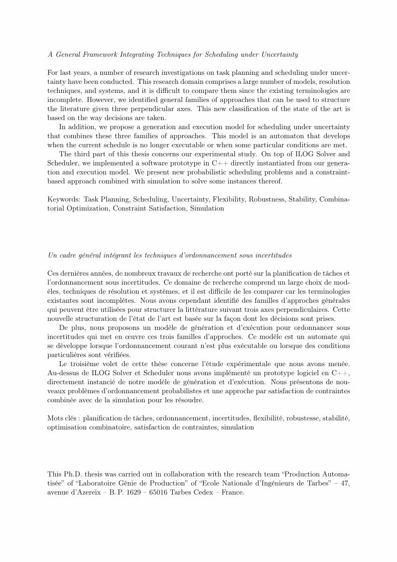
A General Framework Integrating Techniques for Scheduling under Uncertainty
For last years, a number of research investigations on task planning and scheduling under uncer-tainty have been conducted. This research domain comprises a large number of models, resolutiontechniques, and systems, and it is difficult to compare them since the existing terminologies areincomplete. However, we identified general families of approaches that can be used to structurethe literature given three perpendicular axes. This new classification of the state of the art isbased on the way decisions are taken.
In addition, we propose a generation and execution model for scheduling under uncertaintythat combines these three families of approaches. This model is an automaton that developswhen the current schedule is no longer executable or when some particular conditions are met.
The third part of this thesis concerns our experimental study. On top of ILOG Solver andScheduler, we implemented a software prototype in C++ directly instantiated from our genera-tion and execution model. We present new probabilistic scheduling problems and a constraint-based approach combined with simulation to solve some instances thereof.
Keywords: Task Planning, Scheduling, Uncertainty, Flexibility, Robustness, Stability, Combina-torial Optimization, Constraint Satisfaction, Simulation
Un cadre général intégrant les techniques d’ordonnancement sous incertitudes
Ces dernières années, de nombreux travaux de recherche ont porté sur la planification de tâches etl’ordonnancement sous incertitudes. Ce domaine de recherche comprend un large choix de mod-èles, techniques de résolution et systèmes, et il est difficile de les comparer car les terminologiesexistantes sont incomplètes. Nous avons cependant identifié des familles d’approches généralesqui peuvent être utilisées pour structurer la littérature suivant trois axes perpendiculaires. Cettenouvelle structuration de l’état de l’art est basée sur la façon dont les décisions sont prises.
De plus, nous proposons un modèle de génération et d’exécution pour ordonnancer sousincertitudes qui met en œuvre ces trois familles d’approches. Ce modèle est un automate quise développe lorsque l’ordonnancement courant n’est plus exécutable ou lorsque des conditionsparticulières sont vérifiées.
Le troisième volet de cette thèse concerne l’étude expérimentale que nous avons menée.Au-dessus de ILOG Solver et Scheduler nous avons implémenté un prototype logiciel en C++,directement instancié de notre modèle de génération et d’exécution. Nous présentons de nou-veaux problèmes d’ordonnancement probabilistes et une approche par satisfaction de contraintescombinée avec de la simulation pour les résoudre.
Mots clés : planification de tâches, ordonnancement, incertitudes, flexibilité, robustesse, stabilité,optimisation combinatoire, satisfaction de contraintes, simulation
This Ph.D. thesis was carried out in collaboration with the research team “Production Automa-tisée” of “Laboratoire Génie de Production” of “Ecole Nationale d’Ingénieurs de Tarbes” – 47,avenue d’Azereix – B. P. 1629 – 65016 Tarbes Cedex – France.