A Dynamic Theory of Learning and Relationship Lending

Yunzhi Hu Felipe Varas∗

September 1, 2020

Abstract

An entrepreneur borrows from a relationship bank or the market. The bank has

a higher cost of capital but produces private information over time. While the

entrepreneur accumulates reputation as the lending relationship continues, asym-

metric information is also developed between the bank/entrepreneur and the mar-

ket. In this setting, zombie lending is inevitable: once the entrepreneur becomes

sufficiently reputable, the bank will roll over loans even after learning bad news,

for the prospect of future market financing. Zombie lending is mitigated when the

entrepreneur faces financial constraints. Finally, the bank stops producing infor-

mation too early if information production is costly.

Keywords: private learning, experimentation, reputation, relationship banking,

information monopoly, debt rollover, extend and pretend, adverse selection, dy-

namic games

∗Hu: Kenan-Flagler Business School, UNC Chapel Hill; Yunzhi Hu@kenan-flagler.unc.edu. Varas:

Fuqua School of Business, Duke University; felipe.varas@duke.edu. We are grateful to helpful comments

from the Editor, Philip Bond, the Associate Editor, two anonymous referees, Mitchell Berlin, Briana

Chang, Brendan Daley, Jesse Davis, William Fuchs, Paolo Fulghieri, Ilwoo Hwang, Doron Levit, Fei Li,

Andrey Malenko, Igor Makarov, Manju Puri, Raghu Rajan, Jacob Sagi, Matt Spiegel, Yaz Terajima,

Anjan Thakor, Brian Waters, Ji Yan, as well as participants at UNC, Copenhagen Business School,

Colorado, LSE, SFS-Cavalcade, RCFS-CUHK, FTG summer meeting, FTG Rochester Meeting, LBS

summer symposium, Yale SOM, and WFA. The authors have read the Journal of Finance’s disclosure

policy and have no conflicts of interest to disclose.

1 Introduction

Zombie firms – firms whose operating cash flows persistently fall below their interest

payments – are prevalent in the real world. According to a recent study (Banerjee and

Hofmann, 2018), zombie firms make up about 12% of all publicly traded firms across

14 advanced economies. These firms are detrimental to the real economy: they crowd

out credit to their healthy competitors, thereby reducing aggregate productivity and

hindering investment. Zombie lending has long been perceived as the main reason behind

Japan’s “lost decade” in the 1990s (Caballero et al., 2008; Peek and Rosengren, 2005).

More recently, Acharya et al. (2019) and Blattner et al. (2019) show Europe’s economic

recovery from the debt crisis has also been plagued by banks’ lending to zombie firms.

Why do banks extend loans to firms that are likely unable to repay their loan obligations?

One explanation is through the lens of bank capital (e.g., see Bruche and Llobet

(2013)). By extending “evergreening” loans to their impaired borrowers, banks in dis-

tress gamble for resurrection, hoping their borrowing firms regain solvency, or, at least,

can delay taking a balance sheet hit. However, as documented by the Federal Deposit

Insurance Corporation (FDIC), well-capitalized banks also sometimes extend credit to

their distressed relationship borrowers.1 Is zombie lending a natural and inevitable con-

sequence in bank lending?2

In this paper, we build a dynamic model of relationship lending and argue that even

absent concerns about bank capital, zombie lending, or extend and pretend,3 is inevitable

but self-limiting. Our explanation hinges on the assumption that banks and private

lenders have an informational advantage over market-based lenders. Consequently, a

borrower’s reputation typically grows with the length of its lending relationship, because

bad loans are initially liquidated. This growth of reputation in turn gives a bank incentives

to roll over bad loans – evergreening – prior to passing the buck to the market. Therefore,

zombie lending is inevitable. However, if the bank rolls over bad loans all the time, it can

destroy the reputation benefits in the lending relationship and hence the bank’s incentive

to engage in zombie lending in the first place. Therefore, projects that are found to be bad

1For example, FDIC (2017) shows that First NBC Bank, a bank headquartered in New Orleans,Louisiana, and failed in 2017, was considered Well Capitalized from 2006 through February 2015 (p.24). From 2008 through 2016, examiners criticized the bank’s liberal lending practices to financiallydistressed borrowers, such as numerous renewals with little or no repayment of principal, new loans orrenewals with additional advances, and questionable collateral protection. Management extended newloans that were used to make payments on existing loans and to cover current taxes and insurance. FirstNBC also extended loans and allowed proceeds to be used to pay off other delinquent bank loans, againwithout any requirement for principal payments from the borrowers.

2Banerjee and Hofmann (2018) also argue that low interest rates as opposed to weak bank capitalcontribute to the explanation for the rise of zombie lending. The channels though which low interestrates operate are largely unexplored, though.

3We sometimes use “zombie lending,” “extend and pretend,” and “evergreening” interchangeably.They all refer to the lending decisions to borrowers that are known to be in distress. For most of thepaper, we use “extend and pretend.”

2

early on are liquidated, and no liquidation improves a borrower’s reputation or perceived

quality. In this sense, zombie lending is also self-limiting. The liquidation policy offers

banks incentives to extend and pretend for loans that turn out bad later on, because

these bad loans can be pooled with good ones.

Let us be more specific. We model an entrepreneur investing in a long-term, illiquid

project whose quality is either good or bad. A good project should continue to be

financed, whereas a bad project should be immediately liquidated. Initially, the quality

of the project is unknown to everyone, including the entrepreneur herself. She can raise

funding from either the competitive financial market or a bank that will develop into a

relationship. Market financing takes the form of arm’s-length debt so that lenders only

need to break even given their beliefs about the project’s quality. Under market financing,

no information is ever produced. By contrast, if the entrepreneur borrows from a bank,

screening and monitoring will produce “news” about the project’s quality. We model news

arrival as a Poisson event and assume it is only observed by the entrepreneur and the

bank. In other words, the bank and the entrepreneur learn privately about the project’s

quality as time goes by. Meanwhile, all agents, including lenders in the financial market,

can observe the time since the initialization of the project, which will turn out to be the

important state variable. When the bank loan matures, the bank and the entrepreneur

decide to roll it over, to liquidate the project, or to refinance with the market-based

lenders. These decisions depend crucially on the level of the state variable, and they are

the central analysis of the paper.

We show the equilibrium is characterized by two thresholds in time and therefore in-

cludes three stages. In the first stage, a project is liquidated upon learning the bad news,

whereas loans for the other two types will be rolled over. During this period, the average

quality of borrowers who remained with banks improves. Equivalently, remaining bor-

rowers gain reputation from the liquidation decisions of the bad types. These liquidation

decisions are socially efficient, and therefore we name this stage after efficient liquidation.

In the second stage, however, all loans will be rolled over irrespective of the quality. In

particular, the relationship bank will roll over the loan even if it has known the project

is bad: this bank keeps extending the loan to pretend no bad news has occurred, which

is inefficient. This result on banks rolling over bad loans can be interpreted as zombie

lending. Finally, in the last stage, all entrepreneurs will refinance with the market upon

their bank loans maturing – the market-financing stage.

The intuitions for these results are best explained backwards in time. When time

elapsed gets sufficiently long, all entrepreneurs will become sufficiently reputable and

switch to market financing, driven by the assumption that market-based lenders are

competitive and have lower costs of capital. This outcome is the equilibrium in the

last stage. Now, imagine a scenario in which bad news arrives shortly before the last

stage. The relationship bank could liquidate the project, in which case, it receives a low

3

liquidation value. Alternatively, it can roll over the loan and pretend no bad news has

arrived yet. By hiding bad news today, the bank helps the borrower maintain reputation in

order to refinance with the market shortly in the future. Such “extending and pretending”

dominates liquidation, because very soon, the bank will be fully repaid during market

refinancing. In this case, the expected loss will most likely be borne by the market-based

lenders. By contrast, if negative news arrives early on, “extending and pretending” is

much more costly to the bank, due to both large time discounting and the high probability

that before the time reaches the last stage, the project could have matured. If so, the

expected loss will be entirely borne by the relationship bank. Therefore, liquidating the

project is the preferred option.

Our equilibrium highlights three different sources of inefficiency relative to the first-

best benchmark. First, as in standard dynamic lemons problem, a good borrower expe-

riences delay in receiving market financing. Second, a bad borrower is no longer liqui-

dated after the first stage, even though liquidation has a higher social value. Finally, an

uninformed-type borrower refinances with the market in the third stage, which is too soon

compared to the first-best benchmark. Notice this last source of inefficiency is contrary

to that in the dynamic lemons problem: the inefficiency is not the existence of delay but

instead the insufficient delay.

We show that the concern for extend and pretend is mitigated under a financial

constraint, which essentially limits the repayments from the borrower to the bank. In

particular, this constraint leads to scenarios in which a bad project is liquidated, even

though the liquidation value falls below the joint surplus if both parties choose to roll it

over. As a result, the efficient-liquidation period becomes longer, and the extend-and-

pretend period becomes shorter.

Our interpretation of learning is the process of bank screening and monitoring, which

generates useful information on the entrepreneur’s business prospect but cannot be shared

with others in the financial market. Once we endogenize learning as a costly decision, we

show the bank ceases to learn during the efficient-liquidation stage. Intuitively, the benefit

of learning arises because an informed-bad bank could liquidate a bad project for the

liquidation value. This learning benefit vanishes once time passes the efficient-liquidation

stage. This result highlights a new type of hold-up problem in a lending relationship: the

bank under-invests its effort in producing information when it anticipates the borrower

will refinance with the market in the future. Note this result holds even if the relationship

bank has all the bargaining power: it is unable to capture all the surplus – including

current and the future – generated from learning. Knowing so, the bank under-supplies

its effort in producing information.

Our paper is consistent with the existing empirical evidence and anecdotal stories

summarized in subsection 5.2. Moreover, the result on extend and pretend offers a few

testable implications. First, the age distribution of liquidated loans should be left-skewed,

4

and gradually, loan renewals should contain more favorable terms. Second, our interpre-

tation of the market-financing stage includes debt initial public offering, loan sales and

securitization, and anticipated credit-rating upgrades. Our model predicts the positive-

announcement effect associated with loan renewals should be small or even zero if any

of these events happens shortly after the renewal. More broadly, our result implies the

development of financial markets, such as loan sales and securitization, as well as the

improvement in bond market liquidity, can exacerbate zombie lending.

Related Literature

Broadly, our paper is related to three stands of literature. We build on the approach of

dynamic signaling and private learning (Janssen and Roy, 2002; Kremer and Skrzypacz,

2007; Daley and Green, 2012; Fuchs and Skrzypacz, 2015; Grenadier et al., 2014; Atkeson

et al., 2014; Martel et al., 2018; Hwang, 2018; Kaniel and Orlov, 2020). In our model,

news is private, whereas in Daley and Green (2012), news is publicly observable.4 Martel

et al. (2018) and Hwang (2018) also study problems in which sellers become gradually

informed of an asset’s quality. Besides the specific application to relationship banking,

our model has different theoretical implications. First, sellers in these two papers only

choose the time of trading, whereas in our model, the bank is also endowed the option of

liquidation.5 This additional option, which is natural in the banking context, generates

different dynamics and efficiency implications. In our paper, bad types initially choose to

separate through gradual liquidation and only pool with other types once the reputation

is sufficiently high. Whereas delayed trading is always inefficient in these papers, our

paper additionally highlights insufficient delay for the uninformed types and the lack

of liquidation for the bad types. Second, we study the problem in which learning is

costly and endogenous and show how reputation and asymmetric information affect the

incentives of learning. By doing so, we are able to discover a new type of hold-up problem

in banks’ information production.

Our paper is among the first to introduce dynamic learning in the context of bank-

ing (also see Halac and Kremer (2018) and Hu (2017)). We extend previous work in

relationship banking by Diamond (1991b), Rajan (1992), Boot and Thakor (2000), Par-

lour and Plantin (2008), among others, by studying the impact of dynamic learning

and adverse selection on lending relationships. Whereas Diamond (1991a) emphasizes

reputation buildup during bank lending, borrowers are financed with arm’s-length debt,

and lenders’ decisions are myopic, implying lenders will never have incentives to roll

over bad loans. Rajan (1992) studies the tradeoff between relationship-based lending

and arm’s-length debt, without an explicit role of the borrower’s reputation. Chemma-

4Our model also has a public-news process to justify the off-equilibrium belief.5The bank and entrepreneur can be thought of as the seller, whereas market-based lenders are buyers.

5

nur and Fulghieri (1994a) and Chemmanur and Fulghieri (1994b) emphasize the role of

lenders’ reputation in borrowers’ choices between bank versus market financing, whereas

our paper emphasizes the borrowers’ reputation. Parlour and Plantin (2008) study the

secondary market, where a bank may sell loans due to either a negative capital shock or

if the loan is privately known as bad. They show how a liquid secondary market reduces

a bank’s incentive to monitor. Our paper focuses on the dynamics of rolling over loans

and studies dynamic reasons on why and how banks sell loans. Specifically, the concern

for adverse selection is endogenous build-up over time and depends on the borrower’s

reputation. Bolton et al. (2016) study the choice between transaction and relationship

banking under a similar assumption: the relationship bank has a higher cost of capital

but is able to learn the borrower’s type. The paper shows borrowers are willing to pay

the relationship bank higher interest rates during normal times in order to secure funding

during crises. Our paper has a different focus by showing that the superior information

acquired by the relationship bank can result in inefficient zombie lending.

There is also a literature that adopts a dynamic-contracting approach to study rela-

tionship lending. Boot and Thakor (1994) show that a long-term credit contract enables

the lender to use future low interests so that the equilibrium contract does not involve

collateral once the borrower successfully repays a single-period loan. This implies that

collateral usage will decline as relationship duration increases. Verani (2018) builds a

quantitative general-equilibrium model and shows if the borrower has limited commit-

ment, the lender is willing to accept delayed credit payments in exchange for higher

continuation values. Sanches (2010) has a similar message that the optimal dynamic con-

tract features delayed settlement and debt forgiveness. Note that delayed payment and

forgiveness are necessary for borrowers to remain in the lending relationship and repay

in the future. Both features are different from extend and pretend in our model, where

lenders roll over credit to cover bad private news.6

Our explanation for zombie lending differs from existing theories that largely rely

on regulatory capital requirements (Caballero et al., 2008; Peek and Rosengren, 2005).

Rajan (1994) uses a signal-jamming model and explains the phenomenon of rolling over

bad loans by assuming myopic loan officers facing career concerns. In this literature,

terminating a bad loan results in a negative shock to the bank capital, which can trigger

regulatory actions including bank closure (e.g., Kasa et al. (1999)). This can make

banks reluctant to recognize losses by writing off bad loans. In our paper, banks are well

capitalized and zombie lending emerges in equilibrium because banks are forward-looking

instead of myopic. In this sense, our explanation, based on the borrower’s reputation,

complements the existing ones. Similarly, Puri (1999) shows that banks have incentives

6The reason that the relationship bank does not liquidate the borrower is fundamentally different. Inthe dynamic-contracting literature, the bank chooses not to liquidate in order to offer incentives for theborrower to remain in the relationship. In our paper, the bank chooses not to liquidate in order for thebad borrower to leave the relationship by refinancing with others in the future.

6

to certify a bad firm, hoping investors will invest and repay the loan. Her explanation

focuses on the lender’s reputation, whereas our paper highlights the importance of the

borrowing firm’s reputation. Our paper is also related to previous work on debt rollover

by He and Xiong (2012), Brunnermeier and Oehmke (2013), and He and Milbradt (2016).

One related paper is Geelen (2019), who models the dynamic tradeoff of debt issuance

and rollover under asymmetric information. In contrast to this literature, which mostly

studies competitive lenders, we model one lender that becomes gradually informed – the

bank – together with competitive lenders – the market.

2 Model

We consider a continuous-time model with an infinite horizon. An entrepreneur (she)

invests in a long-term project with unknown quality. She borrows from either a bank that

will develop into a relationship or the competitive financial market. Compared to market

financing, bank financing has the advantage of producing valuable information but with

the downside of a higher cost of capital and the possibility of information monopoly.

Below, we describe the model in detail.

2.1 Project

We consider a long-term project that generates a constant stream of interim cash flows

cdt over a period [t, t+ dt]. The project matures at a random time τφ, which arrives at

an exponential time with intensity φ > 0. Upon maturity, the project produces some

random final cash flows, depending on its type. A good (g) project produces cash flows

R with certainty, whereas a bad (b) project produces R with probability θ < 1. With

probability 1−θ, a matured bad project fails to produce any final cash flows. In addition

to the failure in generating the final cash flows, a bad project may also fail prematurely,

in which case it stops generating any cash flows, including both the interim ones and

the final ones. The premature-failure event arrives at an independent exponential time

τη, where η ≥ 0 is the arrival intensity. We sometimes refer to this premature failure as

public news. We assume η is sufficiently low and can be zero, so that none of the main

results depend on this public-news process.

Initially, no agent, including the entrepreneur herself, knows the exact type of the

project; all agents share the same public belief that q0 is the probability of the project

being good. Obviously, if the project fails prematurely, all agents will learn the project is

bad with certainty. At any time before the final cash flows are produced and premature

failure occurs, the project can be terminated with a liquidation value L > 0. Later

in Assumption 1, we impose a parametric assumption that L is higher than the value

of discounted future cash flows generated by a bad project. Therefore, liquidating a

7

bad project will be socially valuable. Note the liquidation value is independent of the

project’s quality, so it should be understood as the liquidation of the physical asset used

in production. For example, one can think of L as the value of the asset if redeployed

(Benmelech, 2009).

Let r > 0 be the entrepreneur’s discount rate; therefore, the fundamental value of the

project to the entrepreneur at t = 0 is given by the discounted value of its future cash

flows:

PV gr =

c+ φR

r + φ, PV b

r =c+ φθR

r + φ+ η, PV u

r = q0PVgr + (1− q0)PV b

r . (1)

Note the denominator of NPV br contains an additional term η, which accounts for the

premature failure event.

Remark 1. Although we do not explicitly model the initial investment, one can imagine

a fixed investment scale I is needed at t = 0 to initialize the project. In subsection 3.3.1,

we derive the maximum amount that an entrepreneur is able to raise at the initial date.

The project is not initialized if this amount falls below I.

2.2 Agents and debt financing

The borrower has no wealth and needs to borrow through debt contracts. The use

of debt contracts is not crucial and can be justified by non-verifiable final cash flows

(Townsend, 1979). One can also interpret these contracts as equity shares with different

control rights and therefore think of the entrepreneur as a manager of a start-up venture.

We consider two types of debt, offered by banks and market-based lenders, respectively.

First, the entrepreneur can take out a loan from a banker (he), who has the same discount

rate r. For tractability reasons, we assume a bank loan lasts for a random period and

matures at a random time τm, upon the arrival of an independent Poisson event with

intensity 1m> 0. m can therefore be interpreted as the expected maturity of the loan.

In most of the analysis, we study the limiting case of instantly maturing loans, that is,

m → 0. Subsection 3.4 solves the case with general m, where results stay qualitatively

unchanged.

The second type of debt is provided by the market and thus can be considered public

bonds. In particular, we consider a competitive financial market in which lenders have

discount rate δ satisfying δ < r. In other words, market financing is cheaper than bank

financing. Regarding (1), let us define the value of the project to the market as

PV gδ =

c+ φR

δ + φ, PV b

δ =c+ φθR

δ + φ+ η, PV u

δ = q0PVgδ + (1− q0)PV b

δ . (2)

The assumption δ < r captures the realistic feature that banks have a higher cost of

8

capital than the market, which can be justified by either regulatory requirements or the

skin in the game needed to monitor borrowers (see Holmstrom and Tirole (1997), e.g.,

and Schwert (2018) for recent empirical evidence). As we clarify shortly, the maturity of

the public debt does not matter, and for simplicity, we assume it only matures with the

project.

Both types of debt share the same exogenously specified face value: F ∈ (L,R).

F > L guarantees debt is risky, whereas F < R captures the wedge between a project’s

maximum income and its pledgeable income (Holmstrom and Tirole, 1998).7 All our

results will go through if F ≡ R, but instead, some non-pledgeable control rents are

accrued to the entrepreneur if the project matures. Note we take F as given: our paper

intends to study the tradeoff between relationship borrowing and public debt, rather than

the optimal leverage. At t = 0, the entrepreneur chooses between public debt and a bank

loan that will develop into a relationship. Once the bank loan matures, she can still

replace it with a public bond. Alternatively, she could roll over the loan with the same

bank, which may have an information advantage over the project’s quality.8 In this case,

the two parties bargain over yt, the interest rate of the loan that is prevalent until the

next rollover date. The financial constraint that the entrepreneur has no wealth restricts

yt to be weakly less than c, the level of the interim cash flows. For the remainder of

this paper, we assume the bank always has all the bargaining power. The results under

interior bargaining power will only differ quantitatively. The allocation of the bargaining

power together with the financial constraint yt ≤ c naturally lead to the result that yt ≡ c.

As we show shortly, this financial constraint limits the size of the repayment that the

entrepreneur can make to the bank; therefore, the Nash bargaining outcome is sometimes

not the one that maximizes the joint surplus of the two.

Because market financing is competitive and market-based lenders have a lower cost

of capital, the entrepreneur will always prefer to take as high leverage as possible once

she borrows from the market. Therefore, the coupon payments associated with the public

bond are cdt.

Remark 2. We have assumed the entrepreneur is only allowed to take one type of debt. In

other words, we have ruled out the possibility of the entrepreneur using more sophisticated

capital structure to signal her type. See Leland and Pyle (1977) and DeMarzo and Duffie

(1999) for these issues.

7The maximum pledgeable cash flow can be microfounded by some unobservable action taken by theentrepreneur (e.g., cash diversion) shortly before the final cash flows are produced (Tirole, 2010).

8We assume without loss of generality that the entrepreneur would never switch to a different bankupon loan maturity. Intuitively, the market has a lower cost of capital than an outsider bank and thesame information structure.

9

2.3 Learning and information structure

The quality of the project is initially unknown, with q0 ∈ (0, 1) being the commonly

shared belief that it is good. If the entrepreneur finances with the bank, that is, if she

takes out a loan, the entrepreneur-bank pair can privately learn the quality of the project

through “news.” Private news arrives at a random time τλ, modeled as an independent

Poisson event with intensity λ > 0. Upon arrival, the news perfectly reveals the project’s

type. In practice, one can think of the news process as information learned during bank

screening and monitoring. We assume such news can only be observed by the two parties

and no committable mechanism is available to share it with third parties, such as credit

bureaus and market participants. In this sense, the news can be understood as soft

information on project quality (Petersen, 2004). For instance, one can think of this news

as the information that banks acquire upon due diligence and covenant violation, which

includes details on the business prospect, collateral quality, and financial soundness of the

borrower. In the benchmark model, we take the learning of private news as exogenous.

Section 4 solves the model in which learning incurs a physical cost, where we show the

bank will only do so in the early stage of a lending relationship.

Although the public-market participants do not observe the private news, they can ob-

serve (1) the public news – whether the project has failed prematurely, (2) t – the project’s

time since initialization, and (3) whether the project has been liquidated. Therefore, the

public can make inference about the project’s quality based on these observations. Let

i ∈ {u, g, b} denote the type of the bank/entrepreneur, where u, g, and b refer to the

uninformed, informed-good, and informed-bad types, respectively. Let µt be the (naive)

belief on the project’s quality if the market lenders solely learn from the fact that the

project has not failed prematurely. A standard filtering result implies

µt = ηµt (1− µt) , (3)

where µ0 = q0. Note the public news could only be bad, which occurs if the project has

failed prematurely.

Let us first describe the private-belief process, that is, the belief held by the bank and

the entrepreneur. If the private news hasn’t arrived yet, the private belief remains at µt.

Upon news arrival at tλ, the private belief jumps to 1 in the case of good news, and 0 if

bad. To characterize the public-belief process, we introduce a belief system{πut , π

gt , π

bt

},

where πut is the public’s belief at time t that the private news hasn’t arrived yet, and

πgt (πbt ) is the public belief that the private news has arrived and is good (bad). In any

equilibrium where the belief is rational, πit is consistent with the actual probability that

the bank and the entrepreneur are of type i ∈ {u, g, b}. Given{πut , π

gt , π

bt

}, the public

10

belief that the project is good is9

qt = πut µt + πgt . (4)

For the remainder of this paper, we sometimes refer to qt as the average quality or the

average belief.

Remark 3. Note that learning and the arrival of private news require joint input from

both the entrepreneur and the bank. Therefore, we can think of learning as exploration

and understanding of the underlying business prospect, which requires the entrepreneur’s

experimentation and the bank’s previous experience in financing related businesses. In

this sense, our model could also be applied to study venture capital firms. Alternatively,

we can interpret learning as a process that solely relies on the entrepreneur’s input,

which is independent of the source of financing, whereas only the bank gets to observe

the news content through monitoring. Put differently, even without bank financing, the

entrepreneur will still be able to learn from news about the quality of her project over

time. Our results in section 3 are identical in this alternative setting, because in the

lending relationship, the bank and the entrepreneur are always equally informed.

2.4 Rollover

When the loan matures, the entrepreneur and the bank have three options: liquidate

the project for L, switch to market financing, or continue the relationship by rolling

over the loan. Control rights are assigned to the bank if the loan is not fully repaid,

and renegotiation could potentially be triggered. Let Oit ≡ Oi

Et + OiBt, i ∈ {u, g, b} be

the maximum joint surplus to the two parties if the loan is not rolled over, where OiEt

and OiBt are the value accrued to the entrepreneur and the bank, respectively. Because

F > L, in the case of liquidation, the bank receives the entire liquidation value L and

the entrepreneur receives nothing, that is, OiBt = L and Oi

Et = 0. If the two parties are

able to switch to market financing, the bank receives full payment OiBt = F , whereas the

entrepreneur receives the remaining surplus OiEt = V i

t − F , where

V gt = Dt +

φ (R− F )

r + φ, V b

t = Dt +φθ (R− F )

r + φ+ η, V u

t = µtVgt + (1− µt) V b

t . (5)

In (5),

Dt = qtDg + (1− qt)Db (6)

is the competitive price of a bond at time t, where Dg = c+φFδ+φ

and Db = c+φθFδ+φ+η

are the

price for the bond of a good- and bad-type project, respectively. qt is the average quality

of the project conditional on refinancing with the market, and in the case in which all

9To simplify notation, we abuse notation and use{πit, qt

}to denote

{πit−, qt−

}.

11

types choose to refinance, qt = qt. The second terms in (5) are the discounted value of the

final cash flows that the entrepreneur i ∈ {u, g, b} receives upon the project’s maturity.

Two conditions need to be satisfied for a loan to be rolled over. First, V it > max

{L, V i

t

}so that rolling over is indeed the decision that maximizes the joint surplus. Second, be-

cause the interest rate of the loan yt cannot go beyond c, the bank needs to prefer rolling

over the loan with interest rate c to liquidating the project for L.

2.5 Strategies and equilibrium

The public history Ht consists of (1) time t, (2) whether the project has failed prema-

turely, and (3) the entrepreneur’s and the bank’s actions up to t. Specifically, it includes

at any time s ≤ t whether the entrepreneur borrows from the bank or the market and

whether the project has been liquidated. For any public history, the price of market debt

Dt summarizes the market lender’s strategy. Given that the market is competitive, the

price of debt satisfies (6).

The private history ht consists of the public history Ht, the rollover event, the Poisson

event on the private-news arrival, and, of course, the content of the news. Essentially,

the strategy of the entrepreneur and the bank is to choose an optimal stopping time,

and at the stopping time, whether to liquidate the project or refinance with the market.

This choice is subject to the additional constraint that at the stopping time, the bank’s

continuation value is at least (weakly) greater than L, the liquidation value of the project.

Let V it be the joint value of the entrepreneur and the bank in the lending relationship, let

Bit the continuation value of the bank,10 and let τ i the (realized) stopping time of type

i i ∈ {u, g, b}.11 We thus have

V ut = max

τu ≥ t,

s.t. Buτu ≥ L

Et−

{∫ τu

t

e−r(s−t)cds+ e−r(τu−t)

[1τu≥τφ

[µτφ +

(1− µτφ

)θ]R + 1τu≥τη · 0

+ 1τu≥τλ[µτλV

gτλ

+ (1− µτλ)V bτλ

]+ 1τu<min{τφ,τλ,τη}max{L, V u

τu}

]},

(7)

12

10We use the standard notation Et−[·] = E[·|ht− ] to indicate the expectation is conditional on thehistory before the realization of the stopping time τ .

11Formally, let tu be the optimal stopping time to liquidate/refinance chosen by type u; then, τu =min {tu, τφ, τη, τλ}. τg and τ b can be similarly defined.

12In the model with general maturity m > 0, τu is restricted to the set of the rollover dates.

12

and

But =Et−

{∫ τu

t

e−r(s−t)cds+ e−r(τu−t)

[1τu≥τφ

[µτφ +

(1− µτφ

)θ]F + 1τu≥τη0

+ 1τu≥τλ[µτλB

gτλ

+ (1− µτλ)Bbτλ

]+ 1τu<min{τφ,τλ,τη}max

{L,min

{V uτu , F

}}]}.

(8)

In (7), τu is the stopping time of the entrepreneur and the bank if both are uninformed.

The first term,∫ τute−r(s−t)cds, is the value of interim cash flows until τu. The project

matures and pays off the final cash flows if τu ≥ τφ. If τu ≥ τη, the project fails

prematurely, with continuation payoff being zero. If τu ≥ τλ, private news arrives, after

which the two parties become informed. Finally, if τu < min {τφ, τη, τλ}, the bank and

the entrepreneur choose to stop before any of the above events arrives, upon which they

either liquidate the project for L or refinance with the market for V uτu . The decision is

made subject to the constraint that Buτu ≥ L. Equation (8) can be interpreted similarly.

The value functions of type g and b are similarly defined in the appendix.

We look for a perfect Bayesian equilibrium of this game.

Definition 1. An equilibrium of the game satisfies the following:

1. Optimality: The rollover decisions are optimal for the bank and the entrepreneur,

given the belief processes {πit, µt, qt}.

2. Belief Consistency: For any history on the equilibrium path, the belief process{πut , π

gt , π

bt

}is consistent with Bayes’ rule.

3. Market Breakeven: The price of the public bond satisfies (6).

4. No (unrealized) Deals:13 For any t > 0 and i ∈ {u, g, b},

V gt ≥ E

[Di|Ht, D

i ≤ Dg]

+φ (R− F )

r + φ

V ut ≥ E

[Di|Ht, D

i ≤ Du]

+ µtφ (R− F )

r + φ+ (1− µt)

φθ (R− F )

r + φ+ η,

where

Du = µtDg + (1− µt)Db.

13We offer a micro-foundation as follows. In each period, two short-lived market-based lenders simul-taneously enter and make private offers to all entrepreneurs. This microfoundation will give rise to theNo-Deals condition as in Daley and Green (2012).

13

5. Belief Monotonicity: Continued bank financing is never perceived as a (strictly)

negative signal, qt ≥ ηqt (1− qt).

The first three conditions are standard. The No-Deals condition follows Daley and

Green (2012), reflecting the requirement that the market cannot profitably deviate by

making an offer that the entrepreneur and the bank will accept. Note the second terms

on the right-hand side of the No-Deals condition reflect the fact that even after market

refinancing, the entrepreneur’s continuation payoff is still type specific.

As is standard in the literature, we use a refinement to rule out unappealing equilibria

that arise due to unreasonable beliefs. Specifically, we impose a belief-monotonicity

refinement that requires that continued bank financing is never perceived as a (strictly)

negative signal. As a result, the public belief about the project’s quality conditional on

bank financing is weakly higher than the naive belief process that is only updated from

the public news that no premature failure has occurred yet. Effectively, this condition

eliminates equilibria that can arise due to threatening beliefs. For example, suppose the

belief is that a project that does not refinance with the market at time t is treated as a

bad type; then, under some conditions, all types will be forced to refinance at time t.

2.6 Parametric assumptions

To make the problem interesting, we make the following parametric assumptions.

Assumption 1. (Liquidation value):

PV bδ < L <

δ + φ

r + φDg +

φθ (R− F )

r + φ. (9)

The first half of Assumption 1 says the liquidation value L is above the discounted

cash flows of a bad project to the market. Therefore, liquidating a bad project is socially

optimal. The second half assumes that if a bad-type borrower can refinance with the

market at a price of a good-type’s bank debt, it will not liquidate the project. Note

this assumption implies L < PV gr , so that continuing a good project is socially optimal.

In the absence of the liquidation option, the equilibrium results are straightforward. In

particular, all types of borrowers will immediately finance with the market at t = 0.14 As

we will see in the next section, this result is no longer true with the option to liquidate.

Assumption 2. (Risky loan):

F > max{θR, L,Db

}. (10)

14The proof follows directly from applying the Law of Iterated Expectation and the assumption thatbank financing is more costly.

14

Assumption 2 assumes the face value of the debt is above the liquidation value, the

expected repayment, and the price of the bond of a bad project; otherwise, the loan is

effectively riskless.

Assumption 3. (Interim cash flow):

c ≥ rF. (11)

Assumption 3 guarantees the size of the interim cash flow c is large enough to com-

pensate the lenders’ cost of capital. Otherwise, the face value of the loan F needs to grow

during rollover dates.

Assumption 4. (Optimal bank financing):

Db <δ + φ

r + φDg (12)

PV bδ <

c+ φθR + λL

r + φ+ λ+ η. (13)

This assumption imposes restrictions so that at least some level of bank financing will

be used in the first-best benchmark. (12) is the static lemons condition in the literature

(Daley and Green, 2012; Hwang, 2018), which requires that the price of a bad-type

bond be lower than the value of a good-type loan. Given Assumption 1, (13) essentially

requires λ to be sufficiently high so that the private news produced during bank financing

is sufficiently useful.

The first-best outcome is achieved if the private news could be publicly observable.

Proposition 1. A unique pair{

¯µFB, µFB

}exists such that in the first-best benchmark,

1. If q0 ≤¯µFB, the unknown project is liquidated at t = 0.

2. If q0 ∈(¯µFB, µFB

), the unknown project is financed with the bank at t = 0.

3. If q0 ≥ µFB, the unknown project is financed with the market at t = 0.

Assumption 1 leads to the result that any good project will immediately receive

financing from the market, whereas a bad project will be liquidated upon news arrival.

According to Proposition 1, an unknown project with belief q0 ∈(¯µFB, µFB

)should start

with bank financing due to the option value of information. Over time, either news or

the premature failure event may arrive, at which point the project receives immediate

market financing following good news and is immediately liquidated following bad news.

In the absence of news and premature failure event, the belief on the project follows (3).

In this case, the project will be financed with the market once µt reaches µFB.

For the remainder of this paper, we assume q0 ∈(¯µFB, µFB

).

15

3 Equilibrium

We solve the model in this section. In subsection 3.1, we study an economy without

the financial constraint that the interest rate of loan satisfies yt ≤ c. The main result is

that an extend-and-pretend region [tb, tg] exists during which the bank will always roll

over the loan, even if it already knows the borrower’s project is bad. Subsection 3.2

studies the equilibrium with a formal treatment of the financial constraint yt ≤ c. We

show the equilibrium structure is similar to the one in subsection 3.1, but the constraint

reduces the length of the extend-and-pretend region. We present a special case without

premature failure in subsection 3.3, where all results are derived in simple and closed

form. Subsection 3.4 further extends the analysis to loans with general maturity and

studies the effect of loan maturity.

3.1 Benchmark without the financial constraint yt ≤ c

The benchmark case without the financial constraint yt ≤ c essentially assumes a

deep-pocked entrepreneur. In particular, the entrepreneur could borrow a loan with the

interest rate yt above c. Given the Nash bargaining assumption at each rollover date, we

can treat the bank and the entrepreneur as one entity, and the problem for the entity

is to choose two optimal stopping times. First, it decides when to liquidate the project.

Second, it decides when to switch to market financing by replacing the loan with the

public debt.

The economy is characterized by state variables in private and public beliefs. All

public beliefs (without liquidation and public news) turn out to be deterministic functions

of the time elapsed. Therefore, we use time t as the state variable. Specifically, we

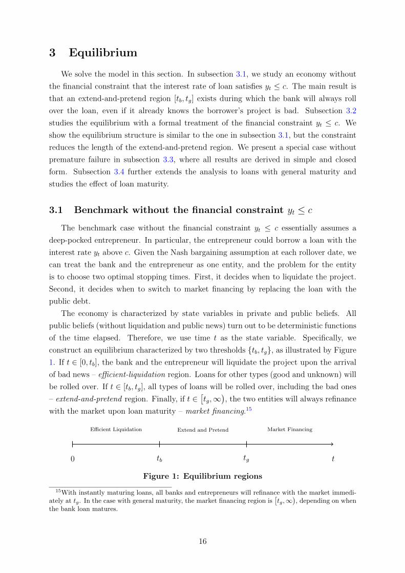
construct an equilibrium characterized by two thresholds {tb, tg}, as illustrated by Figure

1. If t ∈ [0, tb], the bank and the entrepreneur will liquidate the project upon the arrival

of bad news – efficient-liquidation region. Loans for other types (good and unknown) will

be rolled over. If t ∈ [tb, tg], all types of loans will be rolled over, including the bad ones

– extend-and-pretend region. Finally, if t ∈[tg,∞

), the two entities will always refinance

with the market upon loan maturity – market financing.15

0 tb tg t

Efficient Liquidation Extend and Pretend Market Financing

Figure 1: Equilibrium regions

15With instantly maturing loans, all banks and entrepreneurs will refinance with the market immedi-ately at tg. In the case with general maturity, the market financing region is

[tg,∞

), depending on when

the bank loan matures.

16

Given the equilibrium conjecture, the evolution of beliefs follow Lemma 1.

Lemma 1. In an equilibrium with thresholds {tb, tg}, the belief on a project’s average

quality evolves according to

qt =

(λ+ η) qt (1− qt) t ≤ tb

ηqt (1− qt) t > tb(14)

with the initial condition q0.

Heuristically, before t reaches tb, qt evolves as if the premature failure arrives at rate

λ+η, because a project will be immediately liquidated following bad private news. After t

reaches tb, however, qt evolves as if no private news exists at all, because a privately-known

bad project will no longer be liquidated.

Next, we characterize the continuation value in different equilibrium regions, as well

as the boundary conditions. To better explain the economic intuition, we describe the

results backwards in the time elapsed.

Market Financing: {tg}. In this region, V it = V i

t , i ∈ {u, g, b}, where{V ut , V

gt , V

bt

}have been defined in (5) with qt = qt. Let us offer the economic intuition. Ultimately,

if the entrepreneur becomes sufficiently reputable, market financing is cheaper because

market lenders are competitive, and they have a lower cost because δ < r. As a result, all

types will replace their loans with public bonds. The threshold in reputation is obtained

as the public belief qt increases to q. As we show below, this increase is accomplished

because in equilibrium, bad types would have failed prematurely or been liquidated. The

absence of both premature failure and liquidation helps the entrepreneur accumulate

reputation.

Extend and Pretend:[tb, tg

). Working backwards, we now consider the region

[tb, tg

)during which all types of loans, including bad ones, are rolled over. Mathematically, the

value functions of all three types satisfy the following Hamilton-Jacobi-Bellman (HJB)

equation system:

(r + φ+ λ+ (1− µt) η)V ut = V u

t + c+ φ [µt + (1− µt) θ]R + λ[µtV

gt + (1− µt)V b

t

](15a)

(r + φ)V gt = V g

t + c+ φR (15b)

(r + φ+ η)V bt = V b

t + c+ φθR. (15c)

The first term on the right-hand side (15a) is the change in valuation due to time, the

second term captures the benefits of interim cash flow, and the third term corresponds

17

to the event of project maturity, which arrives at rate φ. In this case, the bank and the

entrepreneur receive the final cash flows R with probability µt + (1− µt) θ. The fourth

term stands for the arrival of private news at rate λ. Following the news, the bank and

the entrepreneur become informed. Equations (15b) and (15c) can be interpreted in a

similar vein.

When time gets close to tg, the bank and entrepreneur find that waiting until tg and

refinancing with the market is optimal, even if bad news has arrived. Intuitively, rolling

over bad loans allows the bank to be fully repaid at tg. When time is close to tg, this

decision can be optimal compared to liquidating the project for L. In this region, even

though no project is liquidated, the entrepreneur’s reputation keeps growing as long as

the project does not fail prematurely.

We show tg − tb > 0, implying extend and pretend is inevitable in a dynamic lending

relationship. Equilibrium in this region is clearly inefficient. A bad project should be

liquidated, but instead, the bank and the entrepreneur roll it over in the hope of passing

the losses onto the market lenders at tg. As we see next, by not liquidating between 0

and tb, they have accumulated a good reputation; therefore, extend and pretend can be

sustained in equilibrium.

Efficient Liquidation:[0, tb

)Finally, we turn to the first region

[0, tb

), where bad

loans are not rolled over but instead liquidated. Mathematically, V ut and V g

t are still

described by (15a) and (15b), whereas V bt = L. At the early stage of the lending re-

lationship, only the uninformed and informed-good types roll over maturing loans. By

contrast, a bank that has learned the project is bad chooses to liquidate. Assumption 1

guarantees liquidation possesses a higher value than continuing the project. By continu-

ity, liquidation still has a higher payoff if type b needs to wait for a long time (until tg

in this case) to refinance. As a result, extend and pretend is suboptimal because tg is

far into the future: the firm could likely default or fail prematurely before it reaches the

stage of market financing. The equilibrium is socially efficient in this region. The result

tb > 0 implies the bank cannot extend and pretend all the time. In this sense, extend

and pretend is self-limiting.

Boundary Conditions: The following two boundary conditions are needed to pin

down {tb, tg}:

V btb

= L (16a)

V gtg = ˙V g

tg =(Dg −Db

)ηqtg

(1− qtg

). (16b)

(16a) is the indifference condition for the bad type to liquidate at tb, which is the standard

value-matching condition in optimal stopping problems. In this case, rolling over brings

18

the same payoff L, and thus by continuity and monotonicity, she prefers liquidating when

t < tb and rolling over when t > tb. The second condition, smooth pasting, comes from

the No-Deals condition and the belief monotonicity refinement. We show in the appendix

that if this condition fails, type g will have strictly higher incentives to switch to market

financing before tg. Intuitively, because a bad project’s present value falls below the

liquidation value, the equilibrium decision of refinancing with the market must be one

with pooling. Given the pooling structure in market refinancing, the smooth-pasting

condition solves the optimal-stopping-time problem for the good types. The smooth-

pasting condition picks the earliest tg for the good entrepreneur to refinance with the

market. With the boundary conditions, we can uniquely pin down {tb, tg}, given by the

following proposition.

Proposition 2. A η exists such that if η < η and V u0 ≥ max

{L, V u

0

}, a unique monotone

equilibrium exists in the absence of financial constraints and is characterized by thresholds

tb and tg, where

tb =1

λ+ η

[log

(1− q0

q0

q

1− q

)− η(tg − tb)

](17)

tg − tb =1

r + φ+ ηlog

(V btg − PV

br

L− PV br

), (18)

and q solves

q2 −(

1− r + φ

η

)q +

r + φ

η

(Db

Dg −Db− δ + φ

r + φ

Dg

Dg −Db

)= 0. (19)

The condition η < η is not necessary but helps simplify the expositions. Intuitively, as

η becomes sufficiently low, the No-Deals condition is always slack for the uninformed type

after t = 0 so that they would never be interested in refinancing with only bad types.16

The other condition, V u0 ≥ max

{L, V u

0

}, requires the uninformed type to choose bank

financing at t = 0: the continuation value exceeds both the value of immediate market

financing and liquidation. In the appendix, we provide a closed-form expression for V u0

that allows us to write this condition in term of primitives.

Proposition 2 shows that the length of the extend-and-pretend period (equation (18))

is sufficiently long to deter bad types from mimicking others at tb: whereas V btg − PV

br

captures the additional benefit of extend and pretend until tg, the denominator term in

the logarithm function L−PV br captures the relative benefit of liquidating the project at

tb. Equation (17) shows that the length of the efficient-liquidation period tb gets shorter

16If η becomes very high, the average belief on the uninformed type increases quickly after t = 0 sothat the No-Deals condition for type u may bind after t = 0 even if it holds at t = 0. In other words, theuninformed types’ incentives to pool with bad types can be non-monotonic or even increase over time.These cases are analyzed in the appendix.

19

as public news arrival is more likely (i.e., higher η (tg − tb)) during the extend and pretend

period. Intuitively, when public news is more likely to reveal the project’s type, the repu-

tation of the project grows faster. Therefore, the length of the initial efficient-liquidation

stage, during which reputation grows without liquidation, is necessarily shorter.

Our core mechanism shares similarities with Hwang (2018): on the specific results of

equilibrium in the last two regions, the difference is a matter of equilibrium selection,

which lies between pure strategies and mixed strategies. In absence of external news

(η = 0), our pure-strategy equilibrium is payoff equivalent to the mixed-strategy one

identified there: there is an expected delay in receiving a high offer, whereas in our

paper, the delay in receiving the high offer is deterministic. Moreover, the efficiency

benchmark in our paper is different from existing papers on dynamic lemons market. A

comparison between Propositions 1 and 2 immediately highlights the inefficiencies with

the good and the bad type. Delay in market financing occurs for a good-type project,

which is similar to the standard inefficiency in the dynamic lemons literature. A bad

project is no longer liquidated after tb. Moreover, a comparison between µtg and µFB

highlights an interesting source of inefficiency for the uninformed type. The uninformed

type obtains market financing at tg, which is too soon.17

Corollary 1. Under the parametric conditions in Proposition 2 , µtg < µFB.

Notice this last source of inefficiency is the opposite of the inefficiency in the dynamic

lemons literature: the inefficiency in our model is not the existence of delay, but instead,

the insufficient delay. The uninformed types give up the option value of information after

tg due to the option of market refinancing.

Remark 4. We specify a pessimistic belief during[tb, tg

)off the equilibrium path: any

entrepreneur who seeks market financing during this period will be treated as a bad one

and will be unable to refinance with the market. As in other signaling models, multiple

off-equilibrium beliefs exist that could sustain the equilibrium outcome. The pessimistic

belief is one of them, and perhaps the one most commonly used. In subsection 5.1, we

consider an extension in which the lending relationships may break up exogenously, so

some entrepreneurs always seek market financing on the equilibrium path, and hence

specifying off-equilibrium beliefs is unnecessary. The structure of the equilibrium is sim-

ilar, and we show the equilibrium outcome converges to the one in our model when the

probability of the exogenous breakup goes to zero. We can show that market belief in

the limit is the one that makes the bad type indifferent between rolling over bad loans

and immediately financing with the market, and no discontinuity exists in beliefs at tg.

In other words, the refinement selects an off-equilibrium belief that is continuous in time.

17Note that under η = 0, µtg = q0 so that the result holds trivially. Under continuity, the corollaryholds for η sufficiently small.

20

That said, throughout the paper, we continue to use the pessimistic off-equilibrium belief

because it is more convenient and commonly used in the literature.

3.2 Equilibrium under the financial constraint yt ≤ c

Our benchmark case applies to a scenario in which the Coase theorem holds, so that

frictionless bargaining and negotiation will lead to the efficient allocation between the

entrepreneur and the bank. Therefore, at each rollover date, a loan will be rolled over

if the joint surplus is above the liquidation value L. In this subsection, we formally

analyze the model with the financial constraint yt ≤ c. Clearly, the Coase theorem no

longer applies, and we need to study the incentives of the bank and the entrepreneur

separately.18

The HJBs for the value function {V it , i ∈ {u, g, b}} remain unchanged from those in

subsection 3.1. Again, we can use two thresholds {tb, tg} to characterize the equilib-

rium solutions. Let us now turn to the boundary conditions. First, the smooth-pasting

condition continues to hold, because it selects the equilibrium in which a good-type

entrepreneur chooses to refinance with the market as early as possible. Note the smooth-

pasting condition pins down q, implying the average quality financed by the market

remains unchanged under the financial constraint. The second boundary condition –

value matching at tb – is different. In particular, because the entrepreneur is financially

constrained and cannot repay its loan before tg, the bank has the right to liquidate the

project. It chooses to roll over the loan only if its continuation value lies above L. As a

result, the value-matching condition at tb becomes

Bbtb

= L, (20)

instead of V btb

= L.

Proposition 3. If Bu0 ≥ L, under the financial constraint yt ≤ c and the same parametric

conditions in Proposition 2, the equilibrium is characterized by the two thresholds {tb, tg}

tb =1

λ+ η

[log

(1− q0

q0

q

1− q

)− η(tg − tb)

](21a)

tg − tb =1

r + φ+ ηlog

(F − c+φθF

r+φ+η

L− c+φθFr+φ+η

), (21b)

where q remains unchanged from Proposition 2.

18Another financial constraint exists whereby the bond price at tg must be at least F , implying

q ≥ F−Db

Dg−Db . This condition turns out to always be slack, so we only focus on the constraint yt ≤ c.

21

A comparison of Propositions 2 and 3 shows the financial constraint yt ≤ c mitigates

the inefficiency from extend and pretend.

Corollary 2. The length of the extend-and-pretend period tg − tb becomes shorter under

the financial constraint yt ≤ c. tb becomes larger so that the period of efficient liquidation

becomes longer.

Intuitively, the financial constraint yt ≤ c limits the size of repayments that the

entrepreneur is able to make to the bank. Therefore, the constraint allows the bank’s

continuation value to fall below the liquidation value L, even though the joint surplus

is still above L. As a result, the bad project is liquidated more often, compared to the

case without the financial constraint. Consequently, the length of the zombie-lending

period tg− tb becomes shorter. This result highlights the role of financial constraints and

their interaction with asymmetric information among different types of lenders. Whereas

most of the existing empirical research on zombie lending has emphasized the effect of a

financially constrained bank, our theory offers a new testable implication on the effect of

financially constrained firms in the lending relationship. In particular, our results imply

that as firms become more financially constrained, zombie lending could be mitigated.

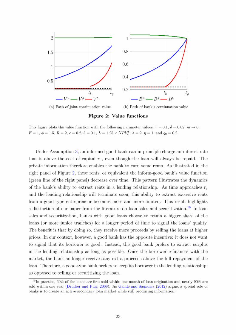
Numerical Example Figure 2 plots the value function of all three types: whereas the

left panel shows the joint valuations of the entrepreneur and the bank, the right one only

shows those of the bank. In this example, tb = 1.2921 and tg = 2.1006. In the figure,

the green, blue, and red lines represent the value functions of the informed-good, the

uninformed, and the informed-bad types, respectively. The dashed horizontal line marks

the levels of L. Before t reaches tb, the bad type’s value function stays at L, and all

the continuation value accrues to the bank. Note that at tb, the bad-type entrepreneur’s

value function experiences a discontinuous jump, whereas no such a jump occurs in the

bank’s value function. This contrast is due to the financial constraint yt ≤ c. Indeed,

both value functions are smooth without this constraint.

22

tb tg

0.5

1

1.5

2

V u V g V b

(a) Path of joint continuation value.

tb tg0.2

0.4

0.6

0.8

1

Bu Bg Bb

(b) Path of bank’s continuation value

Figure 2: Value functions

This figure plots the value function with the following parameter values: r = 0.1, δ = 0.02, m→ 0,

F = 1, φ = 1.5, R = 2, c = 0.2, θ = 0.1, L = 1.25×NPV br , λ = 2, η = 1, and q0 = 0.2.

Under Assumption 3, an informed-good bank can in principle charge an interest rate

that is above the cost of capital r , even though the loan will always be repaid. The

private information therefore enables the bank to earn some rents. As illustrated in the

right panel of Figure 2, these rents, or equivalent the inform-good bank’s value function

(green line of the right panel) decrease over time. This pattern illustrates the dynamics

of the bank’s ability to extract rents in a lending relationship. As time approaches tg

and the lending relationship will terminate soon, this ability to extract excessive rents

from a good-type entrepreneur becomes more and more limited. This result highlights

a distinction of our paper from the literature on loan sales and securitization.19 In loan

sales and securitization, banks with good loans choose to retain a bigger share of the

loans (or more junior tranches) for a longer period of time to signal the loans’ quality.

The benefit is that by doing so, they receive more proceeds by selling the loans at higher

prices. In our context, however, a good bank has the opposite incentive: it does not want

to signal that its borrower is good. Instead, the good bank prefers to extract surplus

in the lending relationship as long as possible. Once the borrower refinances with the

market, the bank no longer receives any extra proceeds above the full repayment of the

loan. Therefore, a good-type bank prefers to keep its borrower in the lending relationship,

as opposed to selling or securitizing the loan.

19In practice, 60% of the loans are first sold within one month of loan origination and nearly 90% aresold within one year (Drucker and Puri, 2009). As Gande and Saunders (2012) argue, a special role ofbanks is to create an active secondary loan market while still producing information.

23

3.3 No Premature Failure

In this subsection, we study a special case of our model in which no premature failures

occur, that is, η ≡ 0. As a result, µt, the (naive) belief update from no premature failure,

will always stay at q0. Proposition 4 shows the results, in which we obtain simple and

closed-form solutions for q and tg − tb.

Proposition 4. If η = 0 so that no premature failure occurs, the equilibrium is charac-

terized by thresholds {q, tb, tg}, where

q =

δ+φr+φ

Dg −Db

Dg −Db(22)

tg − tb =1

r + φlog

(F − c+φθF

r+φ

L− c+φθFr+φ

). (23)

Compared to the case without premature failure (η = 0), the case with premature failure

(η > 0) has a higher q and lower tg − tb.

(22) is a standard result in the dynamic lemons literature,20 which is obtained by

solving qtDg + (1− qt)Db = δ+φ

r+φDg. qtD

g + (1− qt)Db captures the competitive price

of the bond, whereas δ+φr+φ

Dg captures the value of a good-type loan. Therefore, q is the

minimum quality q such that the value of the good-type debt to the bank is equal to

the market’s willingness to pay for the debt of an average entrepreneur. The existence of

premature failure (η > 0) reduces Db and therefore increases q. Moreover, the presence

of premature failure renders extend and pretend by bad types more costly, because the

project could fail during this period. As a result, the period of extend and pretend

gets shorter. Proposition 4 implies that for firms with more transparent governance and

accounting systems, the concern for extend and pretend is mitigated.

Our next corollary shows some interesting comparative static results on the amount

of extend and pretend and credit quality with respect to primitive variables.

Corollary 3. In the case of η = 0, q increases with δ, decreases with r and θ, and is

unaffected by either λ or L. Moreover, tg−tb decreases with r, L, and θ, and is unaffected

by δ or λ.

Let us offer some explanations for the results on r and δ. Note the role of the extend-

and-pretend period is to discourage bad types from mimicking other types at t = tb, as

is clearly seen in (23): whereas F − c+φθFr+φ

captures the additional benefit of extend and

pretend until tg, the denominator term in the logarithm function L− c+φθFr+φ

captures the

relative benefit of liquidating the project at tb.

20See Lemma 3 of Hwang (2018), for example.

24

Intuitively, lower δ is associated with cheaper market financing. Therefore, q, the

average quality of borrowers that are eventually financed by the market, decreases. By

contrast, if the cost of bank financing r becomes cheaper, credit quality q increases.

Intuitively, if the bank’s cost of capital becomes lower, gains from trade with the market

are lower, so a good type only refinances with the market if the average quality becomes

even higher.21

3.3.1 Initial Borrowing

Given that no asymmetric information exists at t = 0, and no bankruptcy cost exists,

the entrepreneur would like to borrow as much as possible at the initial date. Therefore,

without loss of generality, we can assume the loan takes the maximum pledgeable income

F , in which case the entrepreneur is able to raise at most Bu0 initially. If the entrepreneur

needs to invest I at t = 0, the project can only be initiated if Bu0 ≥ I. Proposition 5

describes the closed-form expression of Bu0 .

Proposition 5. In the case of η = 0, the entrepreneur’s maximum borrowing amount at

t = 0 is

Bu0 = q0

[c+ φF

r + φ+ e−(r+φ)tb

(Bgtb− c+ φF

r + φ

)]+ (1− q0)

[c+ φθF + λL

r + φ+ λ+ e−(r+φ+λ)tb

(L− c+ φθF

r + φ+ λ

)], (24)

where

Bgtb

=c+ φF

r + φ+ e−(r+φ)(tg−tb)

(F − c+ φF

r + φ

). (25)

Intuitively, Bu0 in (24) has two components. With probability q0, the project is good,

in which case, the bank is able to receive payments c+φFr+φ

until tg, after which it is fully

repaid. With probability 1− q0, the project turns out bad, and the bank has the option

to liquidate it if the bad private news arrives before tb.

An increase in the cost of bank financing r may increase or decrease Bu0 . On one

hand, all the payments (interim and final repayments) are more heavily discounted when

r increases. On the other hand, both q and tg − tb become lower because the incentive to

extend and pretend is lower. As a result, the entrepreneur is able to refinance with the

market (in which case, the bank is fully repaid) earlier. The overall effect thus depends

on the relative magnitude of these two effects.

An increase in δ may also increase or decrease the initial borrowing amount Bu0 . When

market financing becomes more expensive, q increases, as do tb and tg. However, the effect

21Obviously, if r becomes even lower than δ, the entrepreneur will never refinance with the market,and no extend and pretend period exists.

25

of δ on Bu0 includes two counter-veiling effects. First, if the project turns out to be good,

the bank is able to extract excessive rents for a longer period of time, which increases the

amount that it is willing to lend up front. Second, for the fixed payments, the bank needs

to wait longer to be fully repaid, which decreases the amount that it is willing to lend up

front. In the proof in the appendix, we offer details on conditions that characterize the

monotonicity, where we show that, in general, an increase in δ first decreases and then

increases Bu0 .

3.4 General Maturity

Our analysis so far has focused on the case of instantly maturing loans (m → 0). In

this subsection, we describe the results for the general case where loans have expected

maturity m. We show that all our previous results go through.22 Moreover, we show how

tb, tg − tb, and q vary with loan maturity m. For simplicity, we focus on the case without

premature failure, by taking η = 0.

When loans mature gradually, bad projects are also liquidated gradually as their loans

mature during [0, tb]. In online Appendix B.3.1, Lemma 2 describes the evolution of the

public beliefs without liquidation. Moreover, we can generalize the HJB equation systems

into

(r + φ)V ut = V u

t + c+ φ [q0 + (1− q0) θ]R (26a)

+ λ[q0V

gt + (1− q0)V b

t − V ut

]+

1

mR(V u

t , Vut )

(r + φ)V gt = V g

t + c+ φR +1

mR(V g

t , Vgt ) (26b)

(r + φ)V bt = V b

t + c+ φθR +1

mR(V b

t , Vbt ), (26c)

where

R(V it , V

it ) ≡ max

{0, V i

t − V it , L− V i

t

}. (27)

Note the equations systems are identical to those in (15a)-(15c), except for the last terms,

which account for the event whereby the loan matures. In this case, the bank and the

entrepreneur choose between rolling over the debt (0 in equation (27)), replacing the loan

with the market bond (V it − V i

t in (27)), and liquidating the project (L − V it in (27)).

Note that under general maturity, the entrepreneur in general does not get to refinance

immediately after t reaches tg. Therefore, the expressions for V it are different from (5),

and we supplement them in online Appendix B.3.1.

22Note the market financing region under general maturity m > 0 is[tg,∞

), depending on when the

existing bank loan matures after tg.

26

The boundary conditions are unchanged. Again, we characterize the equilibrium in

three regions.

Proposition 6. If the loan has general maturity m, a unique m∗ exists such that the

equilibrium has three stages if m < m∗. The liquidation threshold is given by

tb = min

t > 0 :q0

(1− q0 + q0e

λt) 1λ−1e

1mt

1 + 1m

∫ t0

(1− q0 + q0eλs)1λ e( 1

m−λ)sds

= q

, (28a)

and q follows (22).

1. Without the financial constraint yt ≤ c,

tg − tb =1

r + φlog

(V btg −

c+φθRr+φ

L− c+φθRr+φ

), (29)

where

V btg =

c+ φR

r + φ−φR (1− θ) + 1

mφ(R−F )(1−θ)

r+φ

r + φ+ 1m

. (30)

2. Under the financial constraint yt ≤ c,

tg − tb =1

r + φlog

(r+φ

r+φ+1/m(c+ φθF + 1

mF )− (c+ φθF )

(r + φ)L− (c+ φθF )

). (31)

A simple comparison with the results in subsection 3.3 shows that when m increases, q

stays unchanged and tb increases, whereas tg− tb decreases.23 Intuitively, q is determined

as the lowest average quality at which a good-type entrepreneur is willing to refinance

with the market. In this case, the condition of market financing is such that good types

receive the identical payoff from staying with the bank and refinancing with the market.

Thus, q doesn’t vary with the maturity of the loan.24 It takes longer for the average

quality to reach q when the maturity m increases, because bad projects are liquidated

less frequently. Therefore, tb increases. Finally, after t reaches tg, bad types take longer

to refinance with the market, and therefore V btg decreases with m. Therefore, a shorter

period tg − tb could still deter bad types from mimicking at tb.

When m > m∗ so that the maturity of the loan becomes sufficiently long, the equi-

librium is characterized by one single time cutoff tbg. From t to tbg, bad projects are

liquidated, whereas market financing occurs right after tbg. The boundary condition is

23tg may increase or decrease, depending on the magnitude of λ and r + φ.24Mathematically, the smooth-pasting condition, V gtg = 0, leads to this result.

27

captured by the value-matching condition V btbg

= L.25 Intuitively, the extend-and-pretend

period is necessary to incentivize the bad types to liquidate early on. When the maturity

of the loan becomes long enough, even if the market-financing stage has arrived, the bad

types still need to wait until the loan matures to refinance with the market. For a higher

m, the expected length of this period increases, so the project is more likely to mature

before the next rollover date.

4 Endogenous Learning

Our analysis has assumed learning and (private) news arrival as an exogenous process,

which happens as long as the entrepreneur has an outstanding loan from the bank. In this

section, we analyze the model in which learning is endogenously chosen by the bank as

a costly decision. We show that the equilibrium structure is still captured by thresholds

{tb, tg}. An interesting result is that even if the cost of learning is very small, the bank

will stop producing information before t reaches tb. Note this result goes through even

if the bank has all the bargaining power in the lending relationship. Therefore, our

analysis highlights a new type of hold-up problem in relationship banking: the bank

under-supplies its effort in producing valuable information.

Throughout this section, we assume η = 0 so that no premature failure occurs. We

present the results with the financial constraint yt ≤ c, and the case without the con-

straints yields qualitatively similar results. The structure of the model stays unchanged

from section 2, except banks must learn the private news by choosing a rate at ∈ [0, 1].

Given at, private news arrives at Poisson rate λat, and our previous analysis corresponds

to the case in which at ≡ 1. Clearly, a higher rate leads to an earlier arrival of private

news in expectation. Meanwhile, learning incurs a flow cost ψat so that a higher rate

is also more costly to the bank. Heuristically, within a short period [t, t+ dt], learning

benefit is λat[q0B

gt + (1− q0)Bb

t −But

]dt: with probability λatdt, private news arrives,

at which time the bank receives a continuation payoff Bgt with probability q0 and Bb

t with

probability 1 − q0. The cost of learning is approximately ψatdt during the same period.

Given the linear structure, the bank’s learning decision follows a bang-bang structure.

Specifically, it chooses maximum learning (at = 1) if and only if

λ[q0B

gt + (1− q0)Bb

t −But

]≥ ψ. (32)

Otherwise, it chooses not to learn at all, and at = 0.

Proposition 7. 1. If ψλ<

1m

(1−q0)

r+φ+ 1m

(L− c+φθF

r+φ

), an equilibrium characterized by {ta, tb, tg}

and ta < tb < tg exists. The bank learns if and only if t < ta.

25The smooth-pasting condition no longer holds. In general,dV g

tbg

dt ≥ 0.

28

2. Otherwise, the bank never learns, and the entrepreneur never borrows from the bank.

Let us offer some intuitions behind Proposition 7. If the bad project no longer gets

liquidated, the value of an uninformed bank is a linear combination of an informed-good

one and an informed-bad one, that is, But = q0B

gt + (1− q0)Bb

t , which is the case after t

reaches tb. As a result, after t reaches tb, the benefit of learning is zero, implying that in

any equilibrium, banks may only learn for t ≤ tb. During [0, tb), when the bad projects

still get liquidated, the value of becoming informed is positive because liquidation avoids

the expected loss generated from a bad project (see Figure 3 for a graphical illustration.),

that is, q0Bgt + (1− q0)L − Bu

t > 0. In this case, information is valuable. The above

proposition shows that if the cost of learning is sufficiently low, the bank learns until

ta. If the cost is relatively high, however, the bank will never learn, and consequently,

entrepreneurs will never choose bank financing.

{ta, tb, tg} are given by the solution to the system of equations (B.7) in the online

appendix. Corollary 4 offers the expression in the limiting case of zero maturity.

Corollary 4. As m→ 0, the thresholds in Proposition 7 converge to

ta =1

λ

[log

(q

1− q

)− log

(q0

1− q0

)]

tb = ta −1

r + φlog

1− ψ/λ

(1− q0)(L− c+φθF

r+φ

)

tg = ta +1

r + φlog

(F − c+φθF

r+φ

L− c+φθFr+φ

).

tb is higher compared to the case with exogenous learning as in Proposition 6.

Bit

b

u

gt > tb

b

u

gt < tb

L

Figure 3: Graphical illustration of learning benefits

Note for t ∈ [ta, tb], the bank chooses not to learn in equilibrium. Off the equilibrium

path, if the bank chose to learn, it would liquidate the project upon bad news. The reason

29

that tb needs to be strictly higher than ta is to generate positive benefits from learning.

When the learning cost ψ → 0, tb converges to ta.

Under endogenous learning, q and tg − tb stay unchanged, whereas tb increases. The

reason is that q is determined by the good type’s indifference condition between bank

financing and market financing, whereas tg − tb is the length of the extend-and-pretend

period that is just sufficient to deter bad types from mimicking others at tb. Because both

q and tg− tb are determined by types that are already informed, they are unaffected when

producing information becomes costly and endogenous. Finally, because less information

is produced when learning becomes costly, bad types are liquidated less often, and the

average quality q0 takes longer to reach q, resulting in a higher tb.

Proposition 7 highlights a new type of hold-up problem in relationship lending that

only emerges in the dynamic setup. Rajan (1992) shows that in a lending relationship, the

entrepreneur has an incentive to underinvest her effort, due to the prospect of renegotia-

tion following private news. Our paper shows the relationship bank will also underinvest

in its effort in producing information, even if the bank has all the bargaining power and

the cost of producing information is infinitesimal (but still positive). The reason is that

the prospect of future market refinancing prevents the bank from capturing all the sur-

plus generated from information production, even though it has all the bargaining power.

Knowing so, the bank under-supplies its effort in producing information.26

Numerical Example Under the same set of parameters as in subsection 3.2 (except for

η = 0), with the additional parameter that ψ = 0.06 and m = 1, we can get ta = 3.8350,

tb = 4.7861, and tg = 5.1352.

Figure 4 illustrates the effect of loan maturity on equilibrium results. The dashed

lines plot the same results under Proposition 6, where private news arrives exogenously.

The differences between the solid and the dashed lines, therefore, capture the contribution

from endogenous leaning. In general, two effects arise when the loan maturity gets longer.

First, longer maturity reduces the option value of new information, because the bank

must wait until the rollover date to act on new information. As a result, the incentive to

produce information should be reduced. Second, longer maturity increases the risk that

banks face by rolling over bad loans, which in turn increases banks’ incentives to learn.

In our numerical exercise, the second effect dominates so that ta, the boundary at which

the bank stops learning, increases as loan maturity increases. Therefore, Bu0 , the amount

of initial borrowing, decreases to compensate for the increased learning cost. The bottom

two panels show that as a result, both tb and tg increase, whereas the difference, tg − tbstays unchanged.27

26Diamond et al. (2020) and Diamond et al. (2019) have a similar flavor that high prospective liquidity(akin to the availability of market financing here) results in reduced corporate governance and bankmonitoring.

27When maturity becomes even longer, the effect becomes non-monotonic. In the extreme case where

30

0.2 0.4 0.6 0.8 10.25

0.3

0.35

0.4

maturity

Bu 0

exogenousendogenous

(a)

0.2 0.4 0.6 0.8 110

10.5

11

11.5

12

maturity

t a

(b)

0.2 0.4 0.6 0.8 110

11

12

13

14

maturity

t b

exogenousendogenous

(c)

0.2 0.4 0.6 0.8 110

11

12

13

14

maturity

t g

exogenousendogenous

(d)

Figure 4: Comparative Statics with Endogenous Learning

This figure plots the value function with the following parameter values: r = 0.1, δ = 0.05, F = 1,

φ = 1.5, R = 2, c = 0.2, θ = 0.1, L = 1.5×NPV br , λ = 0.5, and q0 = 0.2, ψ = 0.025.

5 Extension and Empirical Relevance

5.1 Lending-Relationship Breakups

In practice, lending relationships may break up for reasons independent of the un-

derlying project’s quality. For instance, the relationship may have to be terminated if

the bank experiences shocks that dry up its capital or funding. In this subsection, we

modify the model setup by assuming that with rate χ > 0, the lending relationship breaks

up, upon which the entrepreneur is forced to refinance with the market; otherwise, the

project is liquidated immediately. For simplicity, let us focus on the case without either

the premature failure (η = 0) or the financial constraint yt ≤ c.

Note that with some probability, type u and g refinance with the market. As a result,

the loan never matures, private news is useless, and ta = 0. This latter pattern is captured by the secondcase of Proposition 7, in which bank financing is not used in equilibrium (equivalently, ψ gets very high).

31

the bond price always exists on the equilibrium path. An equilibrium is therefore defined

as in Definition 1 without the refinement of No-Deals and belief monotonicity.

Proposition 8. A¯q exists such that if q0 <

¯q, an equilibrium characterized by thresh-

olds {t`, tb, tg} exists. The decisions of the good and uninformed types are identical to

Proposition 4.

1. If t ∈ [0, t`], bad types liquidate their projects upon learning.

2. If t ∈ [t`, tb], bad types liquidate their projects with probability `t ∈ (0, 1) upon

learning. With probability 1− `t, bad types refinance with the market.

3. If t ∈[tb, tg

), bad types refinance with the market at some rate αt > 0.

4. If t = tg, bad types refinance with the market immediately.

Figure 5 illustrates the equilibrium strategies in Proposition 8, which has the same

qualitative features as the one in subsection 3.1. The equilibrium in this modified game,

however, necessarily involves bad types using mixed strategies. When t ∈ [t`, tb], the bad

types are indifferent between liquidating and refinancing with the market. In equilib-

rium, liquidating happens with probability `t so that the average quality of firms that

refinance with the market lies strictly above q0 on the equilibrium path. Panel 5a plots

the probability of liquidation `t. Note that `t decreases with t during [t`, tb], so that qt+,

the quality of the project conditional market refinancing as well as the bond price stay

constant.

When t ∈[tb, tg

), bad types play a mixed strategy between bank financing and market

financing, implying some degree of extend and pretend exists. Note that bad types cannot

always remain in the lending relationship, because the equilibrium bond price will be too

high. Instead, they voluntarily refinance with the market at a strictly positive rate even

without the exogenous breakup.28 Panel 5b plots γt = αtπbt , the flow rate of bad types that

voluntarily seek market financing without the breakup on[tb, tg

).29 As time increases, γt

decreases.

Panel 5c plots the bond price for borrowers who seek market financing between [0, tg].

The price pattern is consistent with the bad types using mixed strategies in equilibrium.

Between 0 and t`, the price increases as bad types liquidate their projects. The price

becomes a constant between t` and tb so that a bad type is indifferent between liquidation

and market refinancing. After t reaches tb, the bond price needs to increase in order to

make bad types indifferent between bank and immediate market financing.

28Note they cannot refinance with an atomic probability, because the bond price will then fall to Db.29The total flow of bad types is χπbt + γt.

32

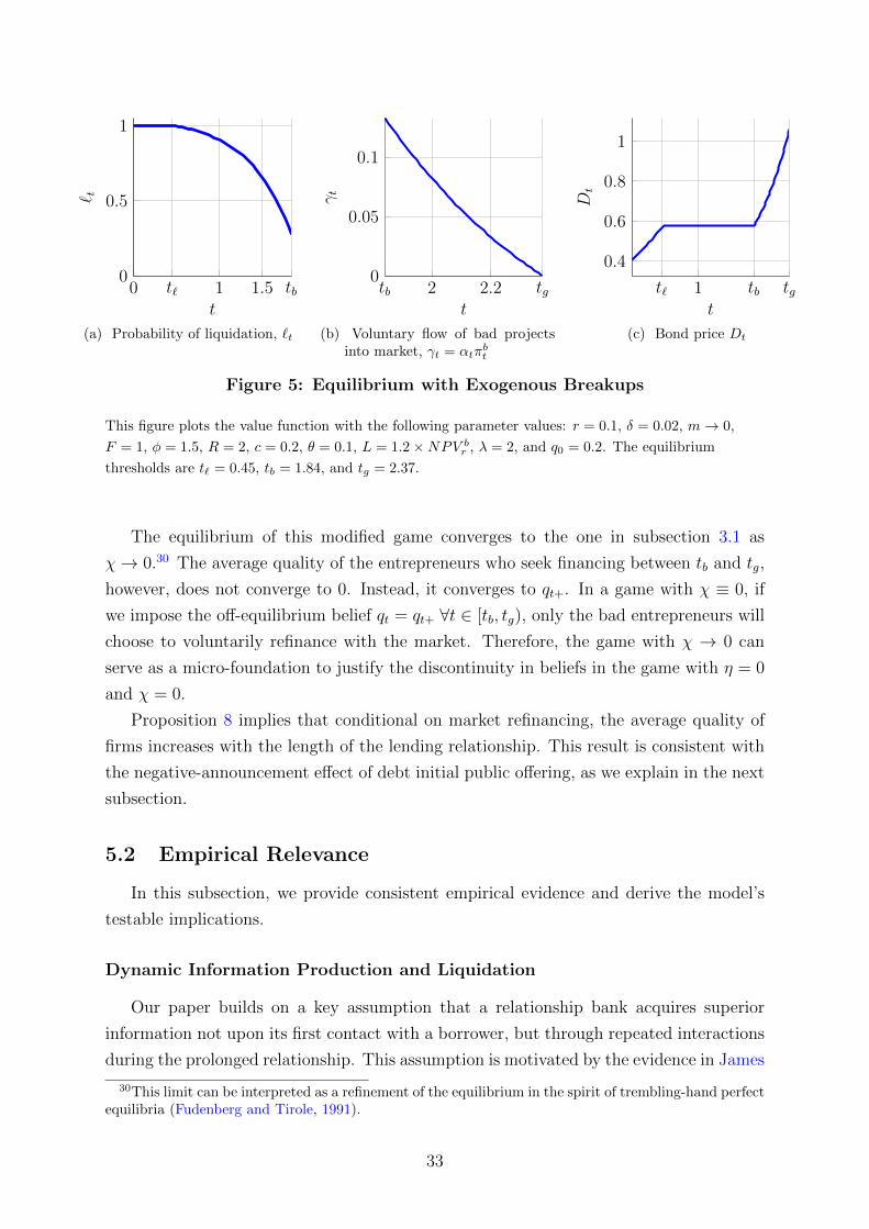
0 t` 1 1.5 tb0

0.5

1

t

` t

(a) Probability of liquidation, `t

2 2.20

0.05

0.1

tb tgt

γt

(b) Voluntary flow of bad projectsinto market, γt = αtπ

bt

t` 1 tb tg

0.4

0.6

0.8

1

t

Dt

(c) Bond price Dt

Figure 5: Equilibrium with Exogenous Breakups

This figure plots the value function with the following parameter values: r = 0.1, δ = 0.02, m→ 0,

F = 1, φ = 1.5, R = 2, c = 0.2, θ = 0.1, L = 1.2×NPV br , λ = 2, and q0 = 0.2. The equilibrium

thresholds are t` = 0.45, tb = 1.84, and tg = 2.37.

The equilibrium of this modified game converges to the one in subsection 3.1 as

χ→ 0.30 The average quality of the entrepreneurs who seek financing between tb and tg,

however, does not converge to 0. Instead, it converges to qt+. In a game with χ ≡ 0, if

we impose the off-equilibrium belief qt = qt+ ∀t ∈ [tb, tg), only the bad entrepreneurs will

choose to voluntarily refinance with the market. Therefore, the game with χ → 0 can

serve as a micro-foundation to justify the discontinuity in beliefs in the game with η = 0

and χ = 0.

Proposition 8 implies that conditional on market refinancing, the average quality of

firms increases with the length of the lending relationship. This result is consistent with

the negative-announcement effect of debt initial public offering, as we explain in the next

subsection.

5.2 Empirical Relevance

In this subsection, we provide consistent empirical evidence and derive the model’s

testable implications.

Dynamic Information Production and Liquidation

Our paper builds on a key assumption that a relationship bank acquires superior

information not upon its first contact with a borrower, but through repeated interactions

during the prolonged relationship. This assumption is motivated by the evidence in James

30This limit can be interpreted as a refinement of the equilibrium in the spirit of trembling-hand perfectequilibria (Fudenberg and Tirole, 1991).

33

(1987) and especially Lummer and McConnell (1989), who find no abnormal returns to the

announcement of new loans, but strong abnormal returns associated with loan renewals.31

Moreover, renewals with favorable (unfavorable) terms have positive (negative) abnormal

returns, suggesting the importance of asymmetric information.32 Our result on extend

and pretend implies that as the lending relationship continues, renewals should gradually

contain more favorable terms, but the positive abnormal returns will shrink. The result

on efficient liquidation predicts the age distribution of liquidated loans is left-skewed.33

Extend and Pretend

A central result of our model is that relationship banks extend and pretend (or conduct

zombie lending) to cover negative private information, so that they can offload these loans

to other lenders in the near future. These other lenders can be non-bank institutions

or other banks with funding advantages. The most direct evidence for this channel is

presented by Gande et al. (1997), who study debt underwriting by commercial banks and

investment houses. They show that when debt securities are issued for purposes other

than repaying existing bank debt, the yield spreads are reduced by 42 basis points if

underwritten by commercial banks. Interestingly, when the stated purpose is to refinance

existing bank debt, there is no statistical significance between yield spreads on debt issues

underwritten by commercial banks and investment houses.

Besides, some anecdotal evidence also suggests the channel highlighted in our paper.

An example is Horizon Bank in Washington, which failed in 2010. According to its

Material Loss Review, Horizon Bank frequently renewed, extended, or modified its large

relationship loans without taking adequate steps to ensure the borrower had the capacity

to repay the loan. Loan files often cited refinancing as the sole exit strategy in the event of

problems (pp. 7 and 9 in FDIC (2010)). In practice, many troubled loans are eventually

refinanced by others, which in some cases even causes the failure of the banks who buy

these loans. An example is FirstCity Bank of Stockbridge in Georgia, which failed in

2009. According to its Material Loss Review, the bank had adopted inadequate loan

policies, and no analysis was made of possible liquidation values in the event a project

did not perform (p. 6 of FDIC (2009)). The Gordon Bank in Georgia, which purchased

many loan participations from FirstCity without performing adequate due diligence,34

31Slovin et al. (1992), Best and Zhang (1993), and Billett et al. (1995) document positive and significantprice reactions to both loan initiation and renewal announcements.

32More recently, Botsch and Vanasco (2019) provide evidence that loan contract terms change overtime as banks learn about borrowers. In particular, relationship lending benefits are heterogeneous,with higher-quality borrowers experiencing declining prices and lower-quality borrowers experiencingincreasing prices and declining credit supply. This evidence is consistent with our key assumption thata relationship bank acquires superior information through repeated transactions with the borrower.

33In practice, bank loans are often secured. It is widely believed that lenders obtain more bargainingpower upon seizing the asset and push for liquidation. See Benmelech et al. (2020) and the citationtherein.

34Loan participation is defined as the transfer of an undivided interest in all or part of the principle

34

subsequently failed in 2011 (FDIC, 2011). Relatedly, Giannetti et al. (2017) show that

for low-quality borrowers with multiple lenders, a relationship bank upgrades its private

credit rating about the borrower in order to avoid other lenders cutting credit and thus

impairing the borrower’s ability to repay loans.35

Market Financing

Our model’s market-financing stage can be interpreted in various ways. The most

direct interpretation is debt initial public offering. Datta et al. (2000) show that initial

public debt offering has a negative stock price effect, and the effect is stronger for younger

firms. Our model with exogenous breakup is consistent this pattern (Panel 5c of Figure 5).

Early on, only bad projects are voluntarily refinanced with the market without lending-

relationship breakups. Only during later stages do the good and uninformed types start to

voluntarily refinance with the market as well. A complementary hypothesis that remains

untested is that the announcement effect of loan renewals preceding public debt issuance

(or loan sales) should be small or even zero. An alternative interpretation of market

financing is a credit-rating upgrade from speculative to investment bucket, which, as

shown by Rauh and Sufi (2010), leads to firms heavily shifting away from bank loans

to bonds. Our model predicts relationship banks are more likely to extend and pretend

before debt initial public offerings and anticipated rating upgrades. Potentially, one can

test whether covenant violations lead to less harsh outcomes during these periods.

More broadly, the market-financing stage can be interpreted as loan sales and securi-

tization.36 In our model, two kinds of loans may be sold: (1) bad loans that banks try to

offload, and (2) good loans for which the borrowers seek cheaper credit in order to relax

their borrowing constraints. Indeed, existing evidence on loan sales and loan quality is

mixed. Dahiya et al. (2003) find negative-announcement effects on loan sales, and almost

half of the borrowers later filed for bankruptcy. Interestingly, these firms are not the

worst-performing firms at the time of loan sales, based on public information such as

return on assets, investment, and leverage, suggesting negative private information con-

tained in loan sales. By contrast, Drucker and Puri (2009) find that sold loans did not

decline in quality. Gande and Saunders (2012) find that a borrowing firm’s stock price

experiences a positive increase on the first day of its loan being traded in the secondary

market, driven by the relaxed financial constraint.37 As acknowledged by Gande and

amount of a loan from a seller, known as the “lead,” to a buyer, known as the “participant,” withoutrecourse to the lead, pursuant to an agreement between the lead and the participant. “Without recourse”means the loan participation is not subject to any agreement that requires the lead to repurchase theparticipants interest or to otherwise compensate the participant upon the borrower’s default on theunderlying loan.

35They also show relationship banks strategically downgrade high-quality borrowers’ ratings.36Note we do not model the security-design problem.37Also see Jiang et al. (2013), who show that loans remaining on a lender’s balance sheet ex post have

higher delinquency rates than those sold. Their explanation is different though.

35

Saunders (2012), in the sample of Dahiya et al. (2003), most original lenders terminated

the lending relationships after the loan sales. Existing studies have documented more

dubious loans being originated (Keys et al., 2010; Bord and Santos, 2015) under secu-

ritization, such as CLOs and CDOs.38 Our paper predicts that as the financial market

develops with the rise of securitization and loan sales (or, equivalently, an improvement

in bond-market liquidity), zombie lending can be a more secular phenomenon. Potentially,

one can verify this pattern using either cross-sectional or time-series data.

6 Concluding Remarks

This paper offers a novel explanation for the prevalent phenomenon of zombie lending.

In particular, we introduce private learning into a banking model and argue that in a

dynamic lending relationship, zombie lending is inevitable but self-limiting. We show

how the length of the zombie-lending period is affected by various factors such as the

cost of bank and market financing, as well as the entrepreneur’s financial constraint.

Moreover, we show that in the dynamic lending relationship, the bank has incentives to

under-supply its effort in producing information.

Our key insights are robust to alternative assumptions. In practice, information about

the borrower’s quality probably arrives in multiple rounds and is imperfect during each

round. The key insights will go through under this alternative assumption. In our model,

the entrepreneur and the bank have incentives to extend and pretend if they know with

certainty that the project is bad. If, instead, they know the project is likely to be

bad (but not with certainty), the cost of rolling over bad loans would be lower, so the

incentives to extend and pretend should be even stronger. Moreover, even though we do

not directly model collateral, L, the liquidation value of the project, can be interpreted

as the collateral value that is redeployed for alternative uses (Benmelech, 2009). Kermani

and Ma (2020) estimate the liquidation recovery rates of assets among US non-financial

firms across industries. In particular, one can think of R − L as the additional cash

flows generated if the project succeeds, and if the project fails, we assume the collateral

value is wiped out. In this sense, the intuition of extend and pretend carries over once

we introduce the role of collaterals. In fact, our results will go through under weaker

assumptions, for instance, if we assume the project generates no cash flows if it fails, but

the collateral value also falls to ξL > 0, where ξ ∈ (0, 1). For ξ sufficiently small, all

our results should carry over. Finally, our extension with exogenous lending-relationship

breakups can be broadly interpreted as shocks to bank capital (Parlour and Plantin,

2008). Results in subsection 5.1 show the key insights will carry over if bank equity is

introduced.

38Benmelech et al. (2012) and Begley and Purnanandam (2017) find the opposite results during adifferent time period.

36

Zombie lending emerges in our paper due to the substitution between the relationship

bank and market-based lenders. An interesting extension is to introduce complementar-

ity between banks and the market as in Song and Thakor (2010). Moreover, we have not

explicitly modeled interbank competition (Boot and Thakor, 2000). Interbank competi-

tion does not change any result in the context of our model, because the new bank is as

uninformed as market-based lenders. Studying the tradeoffs of developing multiple lend-

ing relationships would be interesting. As documented by Farinha and Santos (2002), a

young firm could initiate multiple relationships, because the incumbent bank is unwilling

to extend credit after poor performance.

37

References

Acharya, V. V., T. Eisert, C. Eufinger, and C. Hirsch (2019). Whatever it takes: The

real effects of unconventional monetary policy. The Review of Financial Studies 32 (9),

3366–3411.

Atkeson, A., C. Hellwig, and G. Ordonez (2014). Optimal regulation in the presence of

reputation concerns. The Quarterly Journal of Economics 130 (1), 415–464.

Banerjee, R. and B. Hofmann (2018). The rise of zombie firms: causes and consequences.

BIS Quarterly Review Spetember bb.

Begley, T. A. and A. Purnanandam (2017). Design of financial securities: Empirical

evidence from private-label rmbs deals. The Review of Financial Studies 30 (1), 120–

161.

Benmelech, E. (2009). Asset salability and debt maturity: Evidence from nineteenth-

century american railroads. The Review of Financial Studies 22 (4), 1545–1584.

Benmelech, E., J. Dlugosz, and V. Ivashina (2012). Securitization without adverse selec-

tion: The case of clos. Journal of Financial Economics (1), 91–113.

Benmelech, E., N. Kumar, and R. Rajan (2020). The decline of secured debt. Technical

report, National Bureau of Economic Research.

Best, R. and H. Zhang (1993). Alternative information sources and the information

content of bank loans. The Journal of Finance 48 (4), 1507–1522.

Billett, M. T., M. J. Flannery, and J. A. Garfinkel (1995). The effect of lender identity

on a borrowing firm’s equity return. The Journal of Finance 50 (2), 699–718.

Blattner, L., L. Farinha, and F. Rebelo (2019). When losses turn into loans: the cost of

undercapitalized banks.

Bolton, P., X. Freixas, L. Gambacorta, and P. E. Mistrulli (2016). Relationship and

transaction lending in a crisis. The Review of Financial Studies 29 (10), 2643–2676.

Boot, A. W. and A. V. Thakor (1994). Moral hazard and secured lending in an infinitely

repeated credit market game. International economic review , 899–920.

Boot, A. W. and A. V. Thakor (2000). Can relationship banking survive competition?

The journal of Finance 55 (2), 679–713.

Bord, V. M. and J. A. Santos (2015). Does securitization of corporate loans lead to riskier

lending? Journal of Money, Credit and Banking 47 (2-3), 415–444.

38

Botsch, M. and V. Vanasco (2019). Learning by lending. Journal of Financial Interme-

diation 37, 1–14.

Bruche, M. and G. Llobet (2013). Preventing zombie lending. The Review of Financial

Studies 27 (3), 923–956.

Brunnermeier, M. K. and M. Oehmke (2013). The maturity rat race. The Journal of

Finance 68 (2), 483–521.

Caballero, R. J., T. Hoshi, and A. K. Kashyap (2008). Zombie lending and depressed

restructuring in japan. American Economic Review 98 (5), 1943–77.

Chemmanur, T. J. and P. Fulghieri (1994a). Investment bank reputation, information

production, and financial intermediation. Journal of Finance 49 (1), 57–79.

Chemmanur, T. J. and P. Fulghieri (1994b). Reputation, renegotiation, and the choice

between bank loans and publicly traded debt. Review of Financial Studies 7 (3), 475–

506.

Dahiya, S., M. Puri, and A. Saunders (2003). Bank borrowers and loan sales: New

evidence on the uniqueness of bank loans. The Journal of business 76 (4), 563–582.

Daley, B. and B. Green (2012). Waiting for news in the market for lemons. Economet-

rica 80 (4), 1433–1504.

Datta, S., M. Iskandar-Datta, and A. Patel (2000). Some evidence on the uniqueness of

initial public debt offerings. The journal of finance 55 (2), 715–743.

DeMarzo, P. and D. Duffie (1999). A liquidity-based model of security design. Econo-

metrica 67 (1), 65–99.

Diamond, D., Y. Hu, and R. Rajan (2019). Liquidity and the structure of intermediation.

Technical report, Working paper, University of Chicago.

Diamond, D. W. (1991a). Debt maturity structure and liquidity risk. The Quarterly

Journal of Economics 106 (3), 709–737.

Diamond, D. W. (1991b). Monitoring and reputation: The choice between bank loans

and directly placed debt. Journal of political Economy 99 (4), 689–721.

Diamond, D. W., Y. Hu, and R. G. Rajan (2020). Pledgeability, industry liquidity, and

financing cycles. The Journal of Finance 75 (1), 419–461.

Drucker, S. and M. Puri (2009). On loan sales, loan contracting, and lending relationships.

The Review of Financial Studies 22 (7), 2835–2872.

39

Farinha, L. A. and J. A. Santos (2002). Switching from single to multiple bank lend-

ing relationships: Determinants and implications. Journal of Financial Intermedia-

tion 11 (2), 124–151.

FDIC (2009). Material loss review of firstcity bank, stockbridge, georgia. Report No.

MLR-10-001 .

FDIC (2010). Material loss review of horizon bank, bellingham, washington. Report No.

MLR-10-045 .

FDIC (2011). In-depth review of the failure of the gordon bank, gordon, georgia. Audit

Report No. AUD-11-006 .

FDIC (2017). Material loss review of first nbc bank, new orleans, louisiana. Report No.

AUD-18-002 .

Fuchs, W. and A. Skrzypacz (2015). Government interventions in a dynamic market with

adverse selection. Journal of Economic Theory 158, 371–406.

Fudenberg, D. and J. Tirole (1991). Game Theory. Cambridge, Massachusetts: MIT

Press.

Gande, A., M. Puri, A. Saunders, and I. Walter (1997). Bank underwriting of debt

securities: Modern evidence. The Review of Financial Studies 10 (4), 1175–1202.

Gande, A. and A. Saunders (2012). Are banks still special when there is a secondary

market for loans? The Journal of Finance 67 (5), 1649–1684.

Geelen, T. (2019). Information dynamics and debt maturity. Working Paper, Swiss

Finance Institute.

Giannetti, M., J. M. Liberti, and J. Sturgess (2017). Information sharing and rating

manipulation. The Review of Financial Studies 30 (9), 3269–3304.

Grenadier, S. R., A. Malenko, and I. A. Strebulaev (2014). Investment busts, reputation,

and the temptation to blend in with the crowd. Journal of Financial Economics 111 (1),

137–157.

Halac, M. and I. Kremer (2018). Experimenting with career concerns.

He, Z. and K. Milbradt (2016). Dynamic debt maturity. The Review of Financial Stud-

ies 29 (10), 2677–2736.

He, Z. and W. Xiong (2012). Rollover risk and credit risk. The Journal of Finance 67 (2),

391–430.

40

Holmstrom, B. and J. Tirole (1997). Financial intermediation, loanable funds, and the

real sector. the Quarterly Journal of economics 112 (3), 663–691.

Holmstrom, B. and J. Tirole (1998). Private and public supply of liquidity. Journal of

political Economy 106 (1), 1–40.

Hu, Y. (2017). A dynamic theory of bank lending, firm entry, and investment fluctuations.

Firm Entry, and Investment Fluctuations (August 11, 2017).

Hwang, I. (2018). Dynamic trading with developing adverse selection. Journal of Eco-

nomic Theory 176, 761–802.

James, C. (1987). Some evidence on the uniqueness of bank loans. Journal of financial

economics 19 (2), 217–235.

Janssen, M. C. and S. Roy (2002). Dynamic trading in a durable good market with

asymmetric information. International Economic Review 43 (1), 257–282.

Jiang, W., A. A. Nelson, and E. Vytlacil (2013). Securitization and loan performance:

Ex ante and ex post relations in the mortgage market. The Review of Financial Stud-

ies 27 (2), 454–483.

Kaniel, R. and D. Orlov (2020). Intermediated asymmetric information, compensation,

and career prospects.

Kasa, K., M. M. Spiegel, et al. (1999). The role of relative performance in bank closure

decisions. Federal Reserve Bank of San Francisco.

Kermani, A. and Y. Ma (2020). Asset specificity of non-financial firms. Technical report,

National Bureau of Economic Research.

Keys, B. J., T. Mukherjee, A. Seru, and V. Vig (2010). Did securitization lead to lax

screening? evidence from subprime loans. The Quarterly journal of economics 125 (1),

307–362.

Kremer, I. and A. Skrzypacz (2007). Dynamic signaling and market breakdown. Journal

of Economic Theory 133 (1), 58–82.

Leland, H. E. and D. H. Pyle (1977). Informational asymmetries, financial structure, and

financial intermediation. The journal of Finance 32 (2), 371–387.

Lipster, R. and A. N. Shiryaev (2001). Statistics of Random Processes, II Applications,

2001. Berlin, Heidelberg: Springer.

41

Lummer, S. L. and J. J. McConnell (1989). Further evidence on the bank lending pro-

cess and the capital-market response to bank loan agreements. Journal of Financial

Economics 25 (1), 99–122.

Martel, J., K. S. Mirkin, and B. Waters (2018). Learning by owning in a lemons market.

Available at SSRN 2798088 .

Parlour, C. A. and G. Plantin (2008). Loan sales and relationship banking. The Journal

of Finance 63 (3), 1291–1314.

Peek, J. and E. S. Rosengren (2005). Unnatural selection: Perverse incentives and the

misallocation of credit in japan. American Economic Review 95 (4), 1144–1166.

Petersen, M. A. (2004). Information: Hard and soft.

Puri, M. (1999). Commercial banks as underwriters: Implications for the going public

process. Journal of Financial Economics 54 (2), 133–163.

Rajan, R. G. (1992). Insiders and outsiders: The choice between informed and arm’s-

length debt. The Journal of finance 47 (4), 1367–1400.

Rajan, R. G. (1994). Why bank credit policies fluctuate: A theory and some evidence.

The Quarterly Journal of Economics 109 (2), 399–441.

Rauh, J. D. and A. Sufi (2010). Capital structure and debt structure. The Review of

Financial Studies 23 (12), 4242–4280.

Sanches, D. R. (2010). A dynamic model of unsecured credit.

Schwert, M. (2018). Does borrowing from banks cost more than borrowing from the

market? Available at SSRN 3178915 .

Slovin, M. B., S. A. Johnson, and J. L. Glascock (1992). Firm size and the information

content of bank loan announcements. Journal of Banking & Finance 16 (6), 1057–1071.

Song, F. and A. V. Thakor (2010). Financial system architecture and the co-evolution of

banks and capital markets. The Economic Journal 120 (547), 1021–1055.

Tirole, J. (2010). The theory of corporate finance. Princeton University Press.

Townsend, R. M. (1979). Optimal contracts and competitive markets with costly state

verification. Journal of Economic theory 21 (2), 265–293.

Verani, S. (2018). Aggregate consequences of dynamic credit relationships. Review of

Economic Dynamics 29, 44–67.

42

A Appendix

A.1 Proofs

Let us first supplement the definition for the good and bad types’ value functions.

V gt = max

τ g ≥ t,

s.t. Bgτg ≥ L

Et−

{∫ τg

t

e−r(s−t)cds+ e−r(τg−t)

[1τg≥τφR + 1τg<τφ max{L, V g

τg}

]}

V bt = max

τ b ≥ t,

s.t. Bbτb≥ L

Et−

{∫ τb

t

e−r(s−t)cds+ e−r(τb−t)

[1τb≥τφθR + 1τb≥τη · 0

+ 1τb≤min{τφ,τη}max{L, V b

τb

}]}

Bgt = Et−

{∫ τg

t

e−r(s−t)cds+ e−r(τg−t)

[1τg≥τφF + 1τg<τφ max

{L,min

{V gτg , F

}}]}

Bbt = Et−

{∫ τb

t

e−r(s−t)cds+ e−r(τb−t)

[1τb≥τφθF + 1τb≥τη0

+ 1τb<min{τφ,τη}max{L,min

{V bτb , F

}}]}.

A.1.1 Proof of Proposition 2

Let us first prove the No Deals condition and belief monotonicity requirement imply

smooth pasting at t = tg. That is,

V gtg = Dt = qt(D

g −Db).

The proof follows closely the proof of Theorem 5.1 in Daley and Green (2012). No

Deals and value matching condition immediately implies that V gtg ≤ Dt = qt

(Dg −Db

).

Suppose that V gtg < qt

(Dg −Db

)instead. In this case, consider a deviation in which the

good types wait until tg + ε to refinance with the market, where ε is sufficiently small.

Belief monotonicity implies that qtg+ε is at least (approximately) qtg + ηqtg(1− qtg

)ε,

which shows that the good types have strict incentives to wait until tg + ε.

By applying the smooth pasting and value matching conditions for the type g at the

market financing time t = tg we get

˙V gt =

(Dg −Db

)ηqt (1− qt) .

A1

Using the HJB for the type g during [tb, tg], and letting q = qtg ,

(r + φ)V gt = V g

t + c+ φR

⇒ φ (R− F ) + (r + φ)[qDg + (1− q)Db

]=(Dg −Db

)ηq (1− q) + c+ φR.

Next, we show that given the Assumption 4 there is only one root on [0, 1], which corre-

sponds to the maximal root of the quadratic equation. First, we evaluate LHS − RHSat q = 0:

(r + φ)

(Db − δ + φ

r + φDg

)< 0.

Next, we evaluate LHS −RHS at q = 1:

(r + φ)

(Dg − c+ φF

r + φ

)= (r + φ)

(c+ φF

δ + φ− c+ φF

r + φ

)> 0.

So we can conclude that there is only one root on [0, 1]. Next, we rewrite the quadratic

equation for q as

q2 −(

1− r + φ

η

)q +

r + φ

η

(Db

Dg −Db− δ + φ

r + φ

Db

Dg −Db

)= 0.

Note: the minimum of the quadratic function is attained at

qmin ≡ 1

2

(1− r + φ

η

), (A.1)

and that q > qmin. We will use the observation that q > qmin later to verify the optimality

decisions by different types in equilibrium.

The next step is to solve for the length of tg − tb. Let

D = qDg + (1− q)Db,

and

V btg = D +

φθ (R− F )

r + φ+ η.

Using the boundary condition for the bad type at time tb, Vbtb

= L, together with the

type-b’s HJB equation on [tb, tg]

(r + φ+ η)V bt = V b

t + c+ φθR,

A2

we obtain the equation

tg − tb =1

r + φ+ ηlog

(V btg − PV

br

L− PV br

).

From here, we can find tb using the equation

q =q0

q0 + (1− q0)e−(λ+η)tbe−η(tg−tb),

which yields

tb =1

λ+ η

[log

(1− q0

q0

q

1− q

)− η(tg − tb)

]Optimality the Good Type’s Strategy. We need to verify that it is indeed optimal

for the type g to obtain market financing at time tg. The HJB equation for the high type

on [0, tg).

(r + φ)V gt = V g

t + c+ φR.

To verify that it is not optimal to delay market financing, we need to verify that the

following inequality holds for any t > tg

(r + φ)V gt ≥ ˙V g

t + c+ φR.

On the other hand, to verify that it is not optimal for the good type to seek market

financing before time tg, we need to verify that for any t < tg.

V gt ≥ V g

t .

Next, we proceed to verify each of these inequalities. First, we verify the optimality for

t ≥ tg. Let’s define

Gt = (r + φ)V gt − ˙V g

t − c− φR

= (r + φ)

(Dt +

φ (R− F )

r + φ

)− Dt − c− φR

= (r + φ)Dt − Dt − c− φF

By construction, Gtg = 0 so it is enough to show that Gt ≥ 0 for t > tg. This amounts

to verify that

Gt = (r + φ)Dt − Dt ≥ 0

Substituting the expressions for Dt, we get

Gt = (Dg −Db) [(r + φ)qt − qt] .

A3

In the last region where t ≥ tg, we have qt = ηqt(1− qt) so we get that

Gt = (Dg −Db) [r + φ− η(1− 2qt)] qt.

The conclusion that Gt > 0 follows from the inequality q > qmin, where qmin is defined

in equation (A.1). Next, we verify the optimality for t < tg. Let’s define Ht ≡ V gt − V

gt .

The first step is to show that Ht single crosses zero from above. We have that

Ht = V gt − ˙V g

t

= (r + φ)V gt − c− φR− (Dg −Db)qt

= (r + φ)Ht + (r + φ)V gt − c− φR− (Dg −Db)qt.

Hence, a sufficient condition is

Ht

∣∣∣Ht=0

= (r + φ)V gt − c− φR− (Dg −Db)qt < 0

on (0, tg), which requires that

(r + φ)[qtDg + (1− qt)Db] < (Dg −Db)qt + c+ φF.

Since we have that qt ≥ ηqt (1− qt) and q > qmin, it follows that

(r + φ)[qDg + (1− q)Db] < (Dg −Db)ηq (1− q) + c+ φF,

for all 0 < q < q, which means that Ht

∣∣∣Ht=0

< 0 for t < tg. From here we can conclude

that V gt ≥ V g

t for t < tg.

Optimality of the Bad Type’s Strategy. The strategy of the low type is optimal

if for any t < tb, (r + φ+ η)L ≥ c + φθR ⇒ L ≥ PV br , and for any t ≥ tb, V

bt ≥ L. To

verify that V bt ≥ L for t > tb, notice that on (tb, tg), the value function satisfies

(r + φ+ η)V bt = V b

t + c+ φθR.

This equation can be written as

(r + φ+ η) (V bt − L) = V b

t + c+ φθR− (r + φ+ η)L.

Letting Gt = V bt − L, we obtain the equation

Gt = (r + φ+ η)(Gt + L− PV b

r

), Gtb = 0.

A4

Clearly, Gt

∣∣Gt=0

> 0 so that Gt = V bt − L ≥ 0 for all t ≥ tb.

Optimality of the Uninformed Type’s Strategy. Next, we verify that the unin-

formed is better off rolling over at time t < tb rather than liquidating. First, we solve for

the continuation value of the uninformed at any time t < tb. For t ∈ (0, tb), we have that

(r + φ+ λ+ (1− µt)η)V ut =V u

t + c+ φ [µt + (1− µt) θ]R

+ λ [µtVgt + (1− µt)L]

(r + φ)V gt =V g

t + c+ φR.

Solving backward starting at time tb we get

V ut =

∫ tb

t

e−(r+φ+λ)(s−t)−∫ st η(1−µu)du (c+ φ [µs + (1− µs) θ]R + λ [µsV

gs + (1− µs)L]) ds

+ e−(r+φ+λ)(tb−t)−∫ tbt η(1−µu)duV u

tb

Substituting the relation∫ s

t

η(1− µs)ds =

∫ s

t

µsµsds = log(µs/µt),

and the continuation value of the good type

V gt =

c+ φR

r + φ

(1− e−(r+φ)(tb−t)

)+ e−(r+φ)(tb−t)V g

tb,

we obtain

V ut = µt

[PV g

r + e−(r+φ)(tb−t)(V gtb− PV g

r

)]+ (1− µt)

[c+ φθR + λL

r + φ+ λ+ η+ e−(r+φ+λ+η)(tb−t)

(L− c+ φθR + λL

r + φ+ λ+ η

)]. (A.2)

It is convenient to express the continuation value of the uninformed in terms of the

uninformed’s belief µt. Let t(µ) = − 1η

log(

q01−q0

1−µµ

)be the time at which the belief is µ,

which is given by Let µb be given by t(µb) = tb so

t(µb)− t(µ) = −1

ηlog

(1− µbµb

µ

1− µ

).

A5

Substituting t(µb)− t(µ) we get

V u(µ) = µ

[PV g

r +

(1− µbµb

µ

1− µ

) r+φη (

V gtb− PV g

r

)]

+ (1− µ)

[c+ φθR + λL

r + φ+ λ+ η+

(1− µbµb

µ

1− µ

)1+ r+φ+λη(L− c+ φθR + λL

r + φ+ λ+ η

)]. (A.3)

Letting z ≡ µ/(1− µ), we have that V u(µ) ≥ L if

z

[PV g

r − L+

(z

zb

) r+φη (

V gtb− PV g

r

)]− r + φ+ η

r + φ+ λ+ η

[1−

(z

zb

)1+ r+φ+λη

](L− c+ φθR

r + φ+ λ

)> 0.

The LHS is increasing in z (so V u(µ) is increasing in µ), hence V u(µ) ≥ L for all µ ∈[q0, µb] only if V u(q0) ≥ L.

No Deals for the Uninformed. Finally, we need to verify that the no deals condition

holds for the uninformed type. This is immediate when η = 0, but requires verification

when η > 0. No deals requires that

V ut ≥ Dt + µt

φ(R− F )

r + φ+ (1− µt)

φθ(R− F )

r + φ+ η,

where Dt is the value of debt if the uninformed is pooled with the bad type. In particular,

Dt = qtDg + (1− qt)Db,

where qt is the beliefs conditional on being either uninformed or bad. For t < tb, the

probability of being bad is zero so the probability of the project being good conditional

on being either bad or uninformed is given by

qt = µt =q0

q0 + (1− q0)e−ηt.

For t ∈ (tb, tg) we gave

qt = µtπut

1− πgtwhere

πut =(q0 + (1− q0)e−ηt) e−λt

q0 + (1− q0)e−(λ+η)tbe−η(t−tb)

πgt =q0(1− e−λt)

q0 + (1− q0)e−(λ+η)tbe−η(t−tb)

A6

soπut

1− πgt=

(q0 + (1− q0)e−ηt) e−λt

q0e−λt + (1− q0)e−(λ+η)tbe−η(t−tb)

and

qt =q0e−λt

q0e−λt + (1− q0)e−(λ+η)tbe−η(t−tb)=

q0

q0 + (1− q0)e−λtbe(λ−η)t.

From here we get that Dt is decreasing in time only if λ > η. For any t ∈ [tb, tg], the

continuation value fo the uninformed is given by

V ut = µtV

gt + (1− µt)V b

t .

So the no-deals condition on (tb, tg) can be written as

µt

(V gt −

φ(R− F )

r + φ

)+ (1− µt)

(V bt −

φθ(R− F )

r + φ+ η

)≥ Dt,

where the LHS is increasing in t.

Claim 1.

µt

(V gt −

φ(R− F )

r + φ

)+ (1− µt)

(V bt −

φθ(R− F )

r + φ+ η

)is increasing in time.

Proof. To show that the expression in the proposition is increasing in time, it is sufficient

to show that

V gt − V b

t ≥φ(R− F )

r + φ− φθ(R− F )

r + φ+ η.

At time tg we have

V gt − V b

t =φ(R− F )

r + φ− φθ(R− F )

r + φ+ η,

while at any time t < tg we have

V gt − V b

t = (r + φ)(V gt − V b

t )− ηV bt − φ(1− θ)R.

Solving backward in time starting at tg we get

V gt −V b

t =η

r + φ

c+ φθR

r + φ+ η

(1− e−(r+φ)(tg−t)

)+e−(r+φ)(tg−t)

(1− e−η(tg−t)

)(V btg −

c+ φθR

r + φ+ η

)+φ(1− θ)Rr + φ

(1− e−(r+φ)(tg−t)

)+ e−(r+φ)(tg−t)

(φ(R− F )

r + φ− φθ(R− F )

r + φ+ η

).

A7

Hence, we get that

V gt −V b

t −(φ(R− F )

r + φ− φθ(R− F )

r + φ+ η

)= e−(r+φ)(tg−t)

(1− e−η(tg−t)

)(V btg −

c+ φθR

r + φ+ η

)+

(1− e−(r+φ)(tg−t)

)r + φ+ η

(η

r + φc+ φ(1− θ)F +

η

r + φφF

)> 0.

It follows immediately from the fact that µt, Vbt and V g

t are increasing in time that

µt

(V gt −

φ(R− F )

r + φ

)+ (1− µt)

(V bt −

φθ(R− F )

r + φ+ η

)is also increasing in time.

If λ > η, then the previous claim implies that the it enough to verify the uninformed

no deal’s condition at time tb to guarantee that it is satisfied for all t ∈ [tb, tg]. In which

case, we only need to verify that

µtb

(V gtb− φ(R− F )

r + φ

)+ (1− µtb)

(L− φθ(R− F )

r + φ+ η

)≥ Dtb . (A.4)

At time tb, we have that

qtb =q0

q0 + (1− q0)e−ηtb= µtb ,

thus, we can write condition (A.4) as

µtb

(V gtb−Dg − φ(R− F )

r + φ

)+ (1− µtb)

(L−Db − φθ(R− F )

r + φ+ η

)≥ 0. (A.5)

Therefore, we are only left to verify No Deals on t ∈ [0, tb]. Because qt = µt on (0, tb),

the no-deals condition for the uninformed on (0, tb) condition amounts to verify that

V ut ≥ µt

(Dg +

φ(R− F )

r + φ

)+ (1− µt)

(Db +

φθ(R− F )

r + φ+ η

).

Using equation (A.3), we can write the uninformed’s no-deal condition as

F (z) ≡ z

(z

zb

) r+φη (

V gtb− PV g

r

)+

(z

zb

)1+ r+φ+λη(L− c+ φθR + λL

r + φ+ λ+ η

)− z

(Dg +

φ(R− F )

r + φ− PV g

r

)+c+ φθR + λL

r + φ+ λ+ η− φθ(R− F )

r + φ+ η−Db ≥ 0.

A8

It can be easily verified that F (z) is convex and that its first derivate is given by

F ′(z) =

(1 +

r + φ

η

)(z

zb

) r+φη[(V gtb− PV g

r

)+

1

zb

(L− PV b

r

)]−(Dg +

φ(R− F )

r + φ− PV g

r

).

To verify the no-deals condition we need to consider the case in which the minimum of

F (z) is on the boundary of [z0, zb] and the case in which it is in the interior. Because F (z)

is convex, the previous three cases correspond to: 1) if F ′(z0) ≥ 0, then F is increasing on

[z0, zb] so it is sufficient to check that F (z0) ≥ 0; 2) if F ′(zb) ≤ 0, then F (z) is decreasing

on [z0, zb] so it is sufficient to check that F (zb) ≥ 0; and 3) if F ′(z0) < 0 < F ′(zb),

then F attains its minimum at zmin in the interior of [z0, zb], and we need to verify

that F (zmin) ≥ 0. Notice that F ′(z) > 0 when η → 0, so for η sufficiently small, the

uninformed no deals condition reduces to F (z0) ≥ 0.

Case 1: F ′(z0) ≥ 0. This is the case when

(z0

zb

) r+φη

≥ η

r + φ+ η

(Dg + φ(R−F )

r+φ− PV g

r

)(V gtb− PV g

r

)+ 1

zb(L− PV b

r )

On the other hand, if F ′(z0) ≥ 0, then the uninformed no deals condition is satisfied

if F (z0) ≥ 0. F ′(z0) ≥ 0 if

(z0

zb

) r+φη

>η

r + φ+ η

(Dg + φ(R−F )

r+φ− PV g

r

)(V gtb− PV g

r

)+ 1

zb(L− PV b

r ).

In this case, the uninformed’s no-deals condition is

(z0

zb

) r+φη (

V gtb− PV g

r

)+

[(z0

zb

)1+ r+φ+λη

− 1

]r + φ+ η

r + φ+ λ+ η

(L− PV b

r

)≥

z0

(Dg +

φ(R− F )

r + φ− PV g

r

)+Db +

φθ(R− F )

r + φ+ η− L,

which holds for η sufficiently small. This condition is captured by η < η.

For completeness, we also list the conditions for the other two cases. Note that for η

sufficiently small, these two cases will not show up.

A9

Case 2: F ′(zb) ≤ 0. This is the case when

1 ≤ η

r + φ+ η

(Dg + φ(R−F )

r+φ− PV g

r

)(V gtb− PV g

r

)+ 1

zb(L− PV b

r )

If the previous inequality is satisfied, the uninformed no-deals condition reduces to

F (zb) ≥ 0, which can be written as

V gtb− PV g

r ≥ zb

(Dg +

φ(R− F )

r + φ− PV g

r

)+Db +

φθ(R− F )

r + φ+ η− L.

Case 3: F ′(z0) < 0 < F ′(zb) Finally, if

(z0

zb

) r+φη

<η

r + φ+ η

(Dg + φ(R−F )

r+φ− PV g

r

)(V gtb− PV g

r

)+ 1

zb(L− PV b

r )< 1

then, F (z) attains its minimum in the interior of (z0, zb), and we need to check the

no-deals condition at its minimize. Solving for the first order condition, we find that

zmin = arg minz F (z) is

(zmin

zb

)=

(Dg + φ(R−F )

r+φ− PV g

r

)(

1 + r+φη

) [(V gtb− PV g

r

)+ 1

zb(L− PV b

r )]

ηr+φ

.

Substituting zmin in F (z) we find that the no-deals condition for the uninformed in this

case is

(r + φ)(V gtb− PV g

r

)− (r+φ+η)(r+φ+λ)

r+φ+λ+η1zb

(L− PV b

r

)(1 + r+φ

η

)1+ ηr+φ[(V gtb− PV g

r

)+ 1

zb(L− PV b

r )]1+ η

r+φ

≥ η

zb

Db + φθ(R−F )r+φ+η

− c+φθR+λLr+φ+λ+η(

Dg + φ(R−F )r+φ

− PV gr

)1+ ηr+φ

.

A.1.2 Proof of Proposition 3

The financial constraint is only relevant for the rollover decision. The bank will be

willing to rollover only if Bbt ≥ L. In the equilibrium without the financial constraint,

Bbtb< V b

tb= L. Hence, in the presence of the financial constraint, the boundary condition

for tb is replaced by Bbtb

. By direct computation, we get that the bank’s continuation

value at time tb is given by

Bbtb

=c+ φθF

r + φ+ η

(1− e−(r+φ+η)(tg−tb)

)+ e−(r+φ+η)(tg−tb)F

A10

Solving the boundary condition Bbtb

= L we get

tg − tb =1

r + φ+ ηlog

(F − c+φθF

r+φ+η

L− c+φθFr+φ+η

).

The No-Deals conditions for the good and uninformed type are the same as the un-

constrained case. Hence, the only step left is to analyze the optimality of the rollover

strategy. First, we look at the problem of the low type. In this case, we need to verify

that Bbt ≥ L for t > tb, and that it is not optimal to delay liquidation before time tb. To

verify that Bbt ≥ L on (tb, tg), notice that

(r + φ+ η)Bbt = Bb

t + c+ φθF,

so it follows

Bbt

∣∣∣Bbt=L

= (r + φ+ η)

(L− c+ φθF

r + φ+ η

)> (r + φ+ η)

(L− PV b

r

)> 0,

which immediately implies that Bbt ≥ L for t > tb. To verify that it is not optimal to

delay liquidation on (0, tb), notice that

Bbt + c+ φθF − (r + φ+ η)Bb

t = c+ φθF − (r + φ+ η)L < 0,

which implies that it is optimal to liquidate for t < tb.

Next, we need to verify that the uninformed is willing to rollover the loan at time

t ∈ (0, tb). The continuation value the uninformed satisfies the equation

(r + φ+ λ+ (1− µt)η)But =Bu

t + c+ φ [µt + (1− µt) θ]F

+ λ [µtBgt + (1− µt)L]

(r + φ)Bgt = Bg

t + c+ φF.

Solving backward in time starting at tb, we get that for any t ∈ [0, tb], the uninformed

continuation value is

But = µt

[c+ φF

r + φ+ e−(r+φ)(tb−t)

(Bgtb− c+ φF

r + φ

)]+ (1− µt)

[c+ φθF + λL

r + φ+ λ+ η+ e−(r+φ+λ+η)(tb−t)

(L− c+ φθF + λL

r + φ+ λ+ η

)]. (A.6)

A11

Let us rewrite But in the belief domain:

Bu(µ) = µ

[c+ φF

r + φ+

(1− µbµb

µ

1− µ

) r+φη(Bgtb− c+ φF

r + φ

)]

+ (1− µ)

[c+ φθF + λL

r + φ+ λ+ η+

(1− µbµb

µ

1− µ

)1+ r+φ+λη(L− c+ φθF + λL

r + φ+ λ+ η

)]. (A.7)

The condition But ≥ L can be written in terms of the likelihood ratio z ≡ µ/(1− µ) as

z

[c+ φF

r + φ− L+

(z

zb

) r+φη(Bgtb− c+ φF

r + φ

)]

− r + φ+ η

r + φ+ λ+ η

[1−

(z

zb

)1+ r+φ+λη

](L− c+ φθF

r + φ+ η

)≥ 0.

The left hand side is increasing in z, so it is enough to verify that Bu0 ≥ L.

A.1.3 Proof of Proposition 4 and Corollary 3

Proof. The result on q naturally follows by plugging η = 0 into Proposition 2 and 3. The

result on q and tg − tb follow from Assumption 1 and 4.

A.1.4 Proof of Proposition 5

Proof. Given the boundary conditions, we can show that

Bgtb

=c+ φF

r + φ+ e−(r+φ)(tg−tb)

(F − c+ φF

r + φ

),

whereas Bbtb

= L. When t ∈ [0, tb], the HJB satisfies

(r + φ+ λ)But = Bu

t + c+ φ [q0 + (1− q0) θ]F + λ [q0Bgt + (1− qo)L] .

Solving this ODE, we can write Bu0 in terms of primitives

Bu0 = q0

[c+ φF

r + φ+

(1− qq

q0

1− q0

) r+φλ

(L− c+φθF

r+φ

F − c+φθFr+φ

)rF − cr + φ

]

+ (1− q0)

[c+ φθF + λL

r + φ+ λ+

(1− qq

q0

1− q0

)1+ r+φλ(L− c+ φθF + λL

r + φ+ λ

)].

A12

Finally,

dBu0

d1−qq

= q1+ r+φ

λ0 (1− q0)−

r+φλ ×

(1− qq

) r+φλ−1

×

(L− c+φθF

r+φ

F − c+φθFr+φ

)rF − cr + φ

r + φ

λ+

(L− c+ φθF + λL

r + φ+ λ

)(1 +

r + φ

λ

)(1− qq

),

which is positive if(L− c+φθF+λL

r+φ+λ

) (1 + r+φ

λ

) (1−qq

)>

(L− c+φθF

r+φ

F− c+φθFr+φ

)c−rFr+φ

r+φλ

. Since q in-

creases with δ,dBu0d 1−q

q

> 0 and equivalentlydBu0dδ

< 0 if δ is sufficiently small, whereas

dBu0dδ

< 0 if δ gets sufficiently large.

A.1.5 Proof of Proposition 7 and Corollary 4

We offer the proof for the case without the financial constraint. The proofs for the

case with the financial constraint and Corollary 4 are available in the online appendix.

Define¯ta ≡ 1

λlog(

q1−q

1−q0q0

). The proof is divided in two parts. First, we show that

the equilibrium can be characterized by three thresholds, {ta, tb, tg}, and then we derive

equations determining {ta, tb, tg}.Recall that the boundary conditions for tb and tg are determined by the informed type

b and g, so that endogenous learning will not affect the existence of the three equilibrium

regions, as well as the boundary conditions. It only remains to determine the equilibrium

learning policy by the uninformed type. The first step is to show that the bank never

learns after time tb. The result on [tg,∞) is straightforward, so we will prove that there

is no learning for t ∈ [tb, tg).

Define

Ψt ≡∫ tg

t

e−(r+φ)(s−t)−∫ st λauduψasds

Γt ≡ q0Bgt + (1− q0)Bb

t −But

Suppose that the bank learns during (tb, tg). For any t ∈ (ta, tg), the HJB equation is(r + φ+

1

m

)But = Bu

t + ytF − ψat + φ[q0 + (1− q0)θ]F +1

mV ut + λatΓt (A.8a)(

r + φ+1

m

)Bgt = Bg

t + ytF + φF +1

mV gt (A.8b)(

r + φ+1

m

)Bbt = Bb

t + ytF + φθF +1

mV bt . (A.8c)

A13

The ODE for Γt follows:(r + φ+

1

m+ λat

)Γt = Γt + ψat +

1

m(q0V

gt + (1− q0)V b

t − V ut ) = Γt + ψat +

1

mΨt,

Since Γtg = 0, it implies that λΓt ≤ 0 < ψ for ∀t ∈ [tb, tg]. Therefore, the bank never

learns on t ∈ [tb, tg).

Next, we prove that it if learning happens at all, then it must happen on [0, ta] for

some ta < tb. Let ta = sup{t ≤ tb : λΓt = ψ}. Noticing that Γtb = 0, we can conclude that

ta < tb. We want to show that the optimal policy is at = 1t<ta . Suppose not, then there

is t′a such that λΓt < ψ on (t′a− ε, t′a). In particular, consider t′a = sup{t < ta : λΓt < ψ}.Consider the regions (t′a, ta), in this region, the bank’s HJB equation is(

r + φ+1

m

)But = Bu

t + ytF + φ[q0 + (1− q0)θ]F − ψ +1

mV ut + λΓt(

r + φ+1

m

)Bgt = Bg

t + ytF + φF +1

mV gt(

r + φ+1

m

)Bbt = Bb

t + ytF + φθF +1

mL,

so (r + φ+

1

m+ λ

)Γt = Γt +

1

m(q0V

gt + (1− q0)L− V u

t ) + ψ (A.9)

Let Ht ≡ (1− q0)L+ q0Vgt − V u

t , we get(r + φ+

1

m+ λ

)Γt = Γt +

1

mHt + ψ, t ∈ (t′a, ta)(

r + φ+1

m

)Γt = Γt +

1

mHt, t ∈ (ta, tb).

Taking the left and right limit at t′a we get Γta− = Γta+, so Γt is differentiable at ta. It

follows from the ODE for Γt that if Ht ≤ 0 on (t′a, tb), then Γt is a quasi-convex function

of t on (t′a, tb). To show that Ht ≤ 0, we write an ODE for Ht using the HJB equations

for V bt and V g

t , which is given by

(r + φ+ λ)Ht = Ht + (r + φ) (1− q0)L− (1− q0)(c+ φθR) (A.10)

+ ψ − λ (1− q0) (V bt − L), t ∈ (t′a, ta) (A.11)

(r + φ)Ht = Ht + (r + φ) (1− q0)L− (1− q0)(c+ φθR), t ∈ (ta, tb), (A.12)

where Htb = (1− q0)V btb

+ q0Vgtb− V u

tb= 0. Assumption 1 implies that Htb < 0. Differen-

A14

tiating equation (A.11) and (A.12) we get

(r + φ+ λ) Ht = Ht − λ (1− q0) V bt , t ∈ (t′a, ta)

(r + φ) Ht = Ht, t ∈ (ta, tb).

It immediately follows that Ht = 0 ⇒ Ht ≥ 0 since V bt ≥ 0. Hence, Ht single crosses 0

from negative to positive, so Htb < 0⇒ Ht < 0, ∀t ∈ (t′a, tb).

Since, Γt is quasi-convex on (t′a, tb), Γtb = 0 and Γta = ψ/λ. It must be the case

that Γt′a > ψ/λ, which provides the desired contractions. Thus, it must be the case that

λΓt ≥ ψ for all t < ta

Having shown that the optimal policy is characterized by {ta, tb, tg}, we provide a

solution and derive parametric assumptions needed to validate it. Note that in the

equilibrium characterized by {ta, tb, tg}, beliefs evolve on t ∈ (ta, tb) according to

πut =1

mπut π

bt

πgt =1

mπgt π

bt

πbt = − 1

mπbt(1− πbt

),

which means that the average quality evolves according to

qt =1

mqtπ

bt .

solving the previous equation starting at time ta, we obtain that for any t > ta the average

belief is

qt = qtae1m

∫ ttaπbsds (A.13)

The differential equation for πbt is decoupled from the one for πut and πgt so it can be

solved independently to get

πbt =πbta

πbta + (1− πbta)e1m

(t−ta)

e1m

∫ ttaπbsds =

1− πbt1− πbta

.

Substituting in equation (A.13) we get

qt =1

1− πbta + πbtae− 1m

(t−ta)qta . (A.14)

A15

To find πbta , we use equations (B.9), (B.10), and (B.11) to get:

πbta = 1− qtaq0

(q0 + (1− q0)e−λta

).

Taking the limit of qt in equation (A.14) as t→∞ we get that qt → qta1−πbta

, so limt→∞ qt > q

only if

ta ≥¯ta ≡

1

λlog

(q

1− q1− q0

q0

). (A.15)

Having stablished a lower bound for ta, we proceed to derive a system of equations

for ta, tb, tg. On (ta, tb), the bank’s continuation value satisfies equation (A.8) evaluated

at at = 0. We can solve for Γt using the terminal condition Γtb = 0 to get

Γt =

∫ tb

t

e−(r+φ+ 1m

)(s−t) 1

m[(1− q0)L+ q0V

gs − V u

s ] ds. (A.16)

Te continuation value of the good and the uninformed types can be solved in close form

and are given by for V ut

q0Vgt =

q0c+ q0φR

r + φ(1− e−(r+φ)(tg−t)) + e−(r+φ)(tg−t)q0V

gtg

V ut =

c+ φ [q0 + (1− q0) θ]R

r + φ(1− e−(r+φ)(tg−t)) + e−(r+φ)(tg−t)V u

tg .

Thus, we get that

(1− q0)L+ q0Vgt − V u

t = (1− q0)

[L− c+ φθR

r + φ(1− e−(r+φ)(tg−t))

]+ e−(r+φ)(tg−t)(q0V

gtg − V

utg)

= (1− q0)

[L− c+ φθR

r + φ+ e−(r+φ)(tg−t)

(c+ φθR

r + φ− V b

tg

)]Substituting in equation (A.16) we get

Γt =1m

(1− q0)

r + φ+ 1m

(L− c+ φθR

r + φ

)(1− e−(r+φ+ 1

m)(tb−t)

)+

(1− q0)

(c+ φθR

r + φ− V b

tg

)e−(r+φ)(tg−t)

(1− e−

1m

(tb−t)).

After substituting V btg , we get the following equation for ta:

1m

(1− q0)

r + φ+ 1m

(L− c+ φθR

r + φ

)(1− e−(r+φ+ 1

m)(tb−ta)

)+

(1− q0)

(c+ φθR

r + φ−c+ φθR + 1

mV b

r + φ+ 1m

)e−(r+φ)(tg−ta)

(1− e−

1m

(tb−ta))

=ψ

λ. (A.17)

A16

Combining equations (A.17) and (A.14), together with the incentive compatibility con-

dition determining tg − tb in equation (29), we obtain three equations to characterize the

thresholds: {ta, tb, tg}

q =1

1− πbta + πbtae− 1m

(tb−ta)qta (A.18a)

ψ

λ=

1m

(1− q0)

r + φ+ 1m

(L− PV b

r

) (1− e−(r+φ+ 1

m)(tb−ta)

)+ (1− q0)

(PV b

r −c+ φθR + 1

mV b

r + φ+ 1m

)e−(r+φ)(tg−ta)

(1− e−

1m

(tb−ta))

(A.18b)

tg = tb +1

r + φlog

(V btg − PV

br

L− PV br

). (A.18c)

The final step for the equilibrium to find conditions for an equilibrium with learning

(i.e. ta > 0). Let ta be the threshold the first time qt = q in the benchmark model in which

ψ = 0, which is the same as if ta = tb. On the other hand, if ta = ta ≡ 1λ

log(

q1−q

1−q0q0

)we have that inf{t > ta : qt = q} = ∞. We have already shown that if ta = ta, then

Γta = 0 < ψ/λ. Thus, in any equilibrium ta < ta. Hence, it is sufficient to show that if

ta = ta, then Γta > ψ/λ. We have that limta→ta tg = limta→ta tb =∞, which means that

1m

(1− q0)

r + φ+ 1m

(L− PV b

r

) (1− e−(r+φ+ 1

m)(tg−ta)

)+(1−q0)

(PV b

r −c+ φθR + 1

mV b

r + φ+ 1m

)e−(r+φ)(tg−ta)

(1− e−

1m

(tg−ta))→

1m

(1− q0)

r + φ+ 1m

(L− PV b

r

)Hence, there is ta ∈ (ta, ta) such that λΓt = ψ if and only if

ψ

λ<

1m

(1− q0)

r + φ+ 1m

(L− PV b

r

).

Finally, we can verify that if the previous condition is not satisfied, then there is no

learning in equilibrium. Suppose that the firm never learns and never goes to the market.

In this case, we have the value of the project being

V u = PV ur =

c+ φ(q0 + (1− q0)θ)R

r + φ,

so that the value of bank at loan rate y is

Bu =yF + 1

mV u + φ(q0 + (1− q0)θ)R

r + φ+ 1m

.

Next, suppose that the bank becomes informed (which only occurs off the equilibrium

A17

path). In this case, for any loan rate y, the continuation value fo the good and bad types

are

Bb =y + 1

mL+ φθF

r + φ+ 1m

Bg =y + 1

mV g + φF

r + φ+ 1m

,

where

V g = PV gr .

Combining the previous expressions, we get that

q0Bg + (1− q0)Bb −Bu =

1m

(1− q0)

r + φ+ 1m

(L− PV b

r

),

which means that not learning is optimal if

ψ

λ≥

1m

(1− q0)

r + φ+ 1m

(L− PV b

r

)

A18

B Online Appendix

B.1 Proof of Proposition 1

Given that there is a one-to-one mapping between t and µt if news is publicly observ-

able, we prove this proposition in the time domain. If a project is financed with a bank,

its continuation value satisfies the following HJB equation

(r + φ+ λ+ (1− µt)η)V uFB(t) =V u

FB(t) + c+ φ [µt + (1− µt) θ]R

+ λ [µtPVgδ + (1− µt)L] .

Two boundary conditions characterize µFB = µt=tFB , where tFB is the first-best timing

to switch to market financing. First, the value matching condition holds so that

V uFB(tFB) = µtFBPV

gδ + (1− µtFB)PV b

δ . (B.1)

Second, the smooth-pasting condition holds as tFB is optimally chosen

V uFB(tFB) =

(PV g

δ − PVbδ

)ηµtFB (1− µtFB) . (B.2)

These two conditions pin down the unique solution

µFB =c+ φθR + λL− (r + φ+ λ+ η)PV b

δ

(r + φ)PV gδ − (r + φ+ λ+ η)PV b

δ − φ (1− θ)R + λL.

Assumption 4 guarantees that µFB > 0. Otherwise, bank financing is never used. The

condition PV gδ > c+φR

r+φ≡ PV g

r guarantees that µFB < 1. Finally, V uFB (

¯tFB) = L pins

down the unique solution¯tFB at which µt=

¯tFB =

¯µFB.

For the remainder of the proof, we verify that a policy that seeks market financing

at tFB is optimal. In optimal stopping problems, the value function has to satisfy the

following HJB with variational inequality

max

{V uFB(t) + c+ φ [µt + (1− µt) θ]R + λ [µtPV

gδ + (1− µt)L]

− (r + φ+ λ+ (1− µt)η)V uFB(t), µtPV

gδ + (1− µt)PV b

δ − V uFB(t)

}= 0

In particular, we need to verify for t > tFB

(r + φ+ λ+ (1− µt)η)V uFB(t) ≥ V u

FB(t) + c+ φ [µt + (1− µt) θ]R

+ λ [µtPVgδ + (1− µt)L]

V uFB(t) = µtPV

gδ + (1− µt)PV b

δ ,

A19

while for t < tFB,

(r + φ+ λ+ (1− µt)η)V uFB(t) = V u

FB(t) + c+ φ [µt + (1− µt) θ]R

+ λ [µtPVgδ + (1− µt)L]

V uFB(t) ≥ µtPV

gδ + (1− µt)PV b

δ .

Step 1: Optimality for t > tFB. Let’s define

G(t) ≡ µt(PVgδ − PV

bδ ) + c+ φ [µt + (1− µt) θ]R + λ [µtPV

gδ + (1− µt)L]

− (r + φ+ λ+ (1− µt)η)(µtPV

gδ + (1− µt)PV b

δ

)Smooth pasting plus value matching imply that G(tFB) = 0, and we need to verify that

G(t) ≤ 0 for t > tFB. Thus, it is enough to show that G(t) = 0⇒ G(t) ≤ 0. Substituting

µt = ηµt(1− µt)

in G(t) we get

G(t) = c+ φ [µt + (1− µt) θ]R + λ

[µtc+ φR

δ + φ+ (1− µt)L

]− (r + φ+ λ)

(µtPV

gδ + (1− µt)PV b

δ

)− η(1− µt)PV b

δ .

Differentiating G(t) we get

G(t) =

[φ(1− θ)R + λ

[c+ φR

δ + φ− L

]− (r + φ+ λ)

(PV g

δ − PVbδ

)+ ηPV b

δ

]µt,

and given that µt > 0, the inequality G(t) ≤ 0 reduces to the following condition

φ(1− θ)R + λ

[c+ φR

δ + φ− L

]− (r + φ+ λ)

(PV g

δ − PVbδ

)+ ηPV b

δ ≤ 0

that we can rewrite as

0 ≤ (r + φ)PV gδ − (r + φ+ λ+ η)PV b

δ − φ(1− θ)R + λL,

which holds following Assumption 4.

Step 2: Optimality for t < tFB. Next, we need to show that for t < tFB

V uFB(t) ≥ µtPV

gδ + (1− µt)PV b

δ .

A20

By construction

V uFB(tFB) = µtFBPV

gδ + (1− µtFB)PV b

δ ;

hence, it is enough to show that

V uFB(t)− µtPV g

δ − (1− µt)PV bδ

single crosses zero from above for t < tFB. Let H(t) ≡ V uFB(t) − µtPV g

δ − (1− µt)PV bδ

we get

Ht = V uFB(t)− µt

(PV g

δ − PVbδ

).

Substituting V uFB and µt we get

Ht = (r + φ)V uFB(t)− c− φ [µt + (1− µt) θ]R− λ [µtPV

gδ + (1− µt)L− V u

FB(t)]

− η(1− µt)[µt(PV g

δ − PVbδ

)− V u

FB(t)]

Using the definition of Ht we get

Ht = (r + φ+ λ+ η(1− µt))Ht + (r + φ)(µtPV

gδ + (1− µt)PV b

δ

)− c− φ [µt + (1− µt) θ]R− λ (1− µt) (L− PV b

δ ) + η(1− µt)PV bδ

Thus,

Ht

∣∣∣Ht=0

= (r + φ)(µtPV

gδ + (1− µt)PV b

δ

)− c− φ [µt + (1− µt) θ]R− λ (1− µt) (L− PV b

δ ) + η(1− µt)PV bδ

Rearranging terms we get that Ht

∣∣∣Ht=0

< 0 if and only if

µt < µFB.

Moreover, at time tFB we have Ht = 0. The only step left then is to verify that HtFB > 0

so we can conclude that for any t < tFB we have Ht

∣∣∣Ht=0

< 0, which then implies that

Ht > 0 for all t < tFB. Taking the second derivative we get

Ht

∣∣∣Ht=0,Ht=0

=[(r + φ)PV g

δ − (r + φ+ λ+ η)PV bδ − φ(1− θ)R + λL

]µt > 0

B.2 Proof of Proposition 7 and Corollary 4

We supplement the proof in the case that the entrepreneur is financially constrained.

By similar arguments as the ones in the unconstrained case, the bank never learns after

time tb. Hence, we can restrict attention to the case in which ta < tb. If yt = c, the value

A21

function of the bank satisfies the following HJB equation on (ta, tb)

(r + φ)But = Bu

t + c+ φ[q0 + (1− q0)θ]F (B.3a)

(r + φ)Bgt = Bg

t + c+ φF (B.3b)(r + φ+

1

m

)Bbt = Bb

t + c+ φθF +1

mL. (B.3c)

It follows that Γt satisfies the following ODE

(r + φ)Γt = Γt +1

m(1− q0)(L−Bb

t )

= Γt −1

m(1− q0)

c+ φθF − (r + φ)L

r + φ+ 1m

(1− e−(r+φ+ 1

m)(tb−t)

)(B.4)

Solving equation (B.4) backward in time starting at tb we get

Γt =

∫ tb

t

e−(r+φ)(s−t) 1

m(1− q0)

(r + φ)L− c− φθFr + φ+ 1

m

(1− e−(r+φ+ 1

m)(tb−s)

)ds

=1m

(1− q0)

r + φ

(r + φ)L− c− φθFr + φ+ 1

m

(1− e−(r+φ)(tb−t)

)− (1− q0)

(r + φ)L− c− φθFr + φ+ 1

m

e−(r+φ)(tb−t)(

1− e−1m

(tb−t))

Substituting in the optimality condition λΓta = ψ we get

ψ

λ= (1− q0)

(r + φ)L− c− φθFr + φ+ 1

m

(1m

r + φ

(1− e−(r+φ)(tb−ta)

)− e−(r+φ)(tb−ta)

(1− e−

1m

(tb−ta)))

(B.5)

As before, when ta converges to 1λ

log(

q1−q

1−q0q0

)the threshold tb converges to infinity.

Thus, as in the proof for the unconstrained case, a solution exists if and only if

ψ

λ<

1m

(1− q0)

r + φ+ 1m

(L− c+ φθF

r + φ

)(B.6)

Finally, we need to verify that Γt single crosses ψ/λ. Because Bbt is increasing on (0, tb),

it follows that Γt is quasi-convex on (ta, tb). On (0, ta), Γt satisfies

(r + φ+ λ)Γt = Γt −1

m(1− q0)(Bb

t − L) + ψ.

Again, we can verify that Γt is quasi-convex on (0, ta). Moreover, as Γta− = Γta+, we

can conclude that Γt is quasi-convex on [0, tb]. From here we can conclude that if Γta =

A22

ψ/λ > 0 and Γtb = 0 , then it must be the case that Γt ≤ ψ/λ on (ta, tb). On the other

hand, if there is ta < ta such that Γta < ψ/λ, then it must be that case that Γt has local

maximum on [0, tb). However, this cannot be the case as Γt is quasi-convex. We can

conclude that Γt ≥ ψ/λ for all t < ta.

The rest of the equilibrium is determined as in the case with exogenous learning. The

threshold ta must be such qtb = q, where qt is given by equation (A.14), while tg − tb

is given by equation (31). Summarizing, the equilibrium thresholds are given by the

solution to equations

q =1

1− πbta + πbtae− 1m

(tb−ta)qta (B.7a)

ψ

λ= (1− q0)

(r + φ)L− c− φθFr + φ+ 1

m

(1m

r + φ

(1− e−(r+φ)(tb−ta)

)− e−(r+φ)(tb−ta)

(1− e−

1m

(tb−ta)))

(B.7b)

tg = tb +1

r + φlog

r+φ

r+φ+ 1m

(c+ φθF + 1mF )− (c+ φθF )

(r + φ)L− (c+ φθF )

. (B.7c)

Corollary 4 follows by taking the limit m→ 0.

B.3 General Maturity

B.3.1 Proof of Proposition 6

Lemma 2. Without liquidation, the public beliefs (πut , πgt , π

bt ) satisfy the following differ-

ential equation:

πut = −λπut + 1t≤tb1

mπut π

bt (B.8a)

πgt = λπut q0 + 1t≤tb1

mπgt π

bt (B.8b)

πbt = λπut (1− q0)− 1t≤tb1

mπbt(1− πbt

). (B.8c)

Proof. The evolution of beliefs can be derived directly in continuous time using the filter-

ing formulas for counting processes in Lipster and Shiryaev (2001), examples 2 and 3 in

Chapter 19. Here, we provide a heuristic derivation starting in discrete time and taking

the continuous time limit. Using Baye’s rule we get

πgt =πgt−h + πut−hq0λh

πgt−h + πut−hq0λh+ πut−h(1− λh) +(πbt−h + πut−h(1− q0)λh

)(1− 1

mh),

A23

so

πgt − πgt−h

h=

λq0πut−h + 1

mπgt−hπ

bt−h

πgt−h + πut−hq0λh+ πut−h(1− λh) +(πbt−h + πut−h(1− q0)λh

)(1− 1

mh)

+O(h2)

h.

Taking the limit when h→ 0, we get

πgt = λq0πut +

1

mπgt π

bt . (B.9)

Similarly, we have that

πut =(1− λh)πut−h

πgt−h + πut−hq0λh+ πut−h(1− λh) +(πbt−h + πut−h(1− q0)λh

)(1− 1

mh),

so

πut − πut−hh

=−λπut−h + 1

mπut−hπ

bt−h

πgt−h + πut−hq0λh+ πut−h(1− λh) +(πbt−h + πut−h(1− q0)λh

)(1− 1

mh)

+O(h2)

h.

Taking the limit as h→ 0 we get

πut = −λπut +1

mπut π

bt . (B.10)

Finally, using equations (B.9) and (B.10), together with πbt + πut + πbt = 1, we get

πbt = λ(1− q0)πut −1

mπbt (1− πbt ). (B.11)

Under general maturity,

V gt =

c+ φR

r + φ+ 1m

+1m

r + φ+ 1m

[D +

φ (R− F )

r + φ

]V bt =

c+ φθR

r + φ+ 1m

+1m

r + φ+ 1m

[D +

φθ (R− F )

r + φ

]V ut = q0V

gt + (1− q0) V b

t .

The final step is to find the solution for qt in the interval [0, tb]. Let us define in this proof

A24

zt =πgtπut

, then,

zt =πgt π

ut − π

gt π

ut

(πut )2=πgtπut− zt

πutπut

= λq0 +1

mzt (1− πgt − πut )− zt

(−λ+

1

m(1− πgt − πut )

)= λ (q0 + zt) .

Therefore, we have the solution

zt = q0

(eλt − 1

)⇒ πgt = q0

(eλt − 1

)πut . (B.12)

Since πut + πgt + πbt = 1, we also have

πbt = 1−(q0e

λt + 1− q0

)πut . (B.13)

Substituting (B.12) and (B.13) into the ODE system, we get a first-order ODE for πut

πut =

(1

m− λ)πut −

1

m

(q0e

λt + 1− q0

)(πut )2 ,

which corresponds to a continuous-time Riccati equation. This equation can be trans-

formed it into a second-order ODE. In this proof, let vt = − 1m

(q0e

λt + 1− q0

)πut and

Qt = q0eλt + 1− q0,

vt = v2t +

vtQt

[q0e

λtλ+Qt

(1

m− λ)]

. (B.14)

Further, if we let vt = − νtνt⇒ vt = − νt

νt+ (vt)

2, then we can transform equation (B.14)

into the following second-order ODE

νt =νtQt

[q0e

λtλ+Qt

(1

m− λ)]

From here, we get that

νt = ν(0)e

∫ t0 λ

1

1+1−q0q0

e−λsds+( 1

m−λ)t

Moreover, ∫ t

0

1

1 + 1−q0q0e−λs

ds =1

λlog(1− q0 + q0e

λt)

so

νt = ν(0)(1− q0 + q0e

λt) 1λ e( 1

m−λ)t

A25

Integrating one more time, we get

νt = ν(0) + ν(0)

∫ t

0

(1− q0 + q0e

λs) 1λ e( 1

m−λ)sds.

Using the definition of vt and νt, we have

ν0 = −v0ν(0) =1

mν(0)

so

νt = ν(0)

(1 +

1

m

∫ t

0

(1− q0 + q0e

λs) 1λ e( 1

m−λ)sds

).

Using the definition of vt we get

vt = −1m

(1− q0 + q0e

λt) 1λ e( 1

m−λ)t

1 + 1m

∫ t0

(1− q0 + q0eλs)1λ e( 1

m−λ)sds

so

πut =

(1− q0 + q0e

λt) 1λ−1e( 1

m−λ)t

1 + 1m

∫ t0

(1− q0 + q0eλs)1λ e( 1

m−λ)sds

(B.15)

Thus, substituting (B.15) in the definition for qt, we get

qt = πgt + q0πut

= q0

(eλt − 1

)πut + q0π

ut

= q0eλtπut

=q0

(1− q0 + q0e

λt) 1λ−1e

1mt

1 + 1m

∫ t0

(1− q0 + q0eλs)1λ e( 1

m−λ)sds

(B.16)

Because qt is monotone, the solution for tb and tg is unique.

The result with the financial constraint is similar except for the boundary condition.

q and tb is unchanged, whereas tg − tb is determined by Bbtb

= L.

Finally, the case with and without the financial constraint both require tg − tb > 0,

which pins down the solution of m∗. When m > m∗, the equilibrium does not have the

extend and pretend region.

B.4 Lending-Relationship Breakups

B.4.1 Proof of Proposition 8

Proof. With χ > 0, there is always some probability that good types and informed seek

market financing, so the price of the bond is higher than Db on the equilibrium path.

Let us first describe the equilibrium belief under the conjectured equilibrium strate-

A26

gies. For any t ∈ [0, tb], conditional on the lending relationship continuing, the market

knows for sure that the entrepreneur is not bad, and that it can only be a good type or

an uninformed (that is, πbt = 0, ∀t ∈ [0, tb]). Let qt+ be the average quality of borrower

conditional on refinancing with the market. Clearly, for t ∈ [0, tb]

qt+ =χ

χ+ λ (1− qt) (1− `t)qt.

For t ∈ [tb, tg), conditional on staying with the bank, beliefs evolve according to

πut = −λπut + αtπut π

bt

πgt = λπut q0 + αtπgt π

bt

πbt = λπut (1− q0)− αtπbt(1− πbt

).

qt = πgt + q0πut = αtπ

btqt.

Let us define{πut+, π

gt+, π

bt+, qt+

}as the beliefs conditional on market financing, which

follows

πut+ =χπut

χ+ αtπbt

πgt+ =χπgt

χ+ αtπbt

πbt+ =(χ+ αt)π

bt

χ+ αtπbt

qt+ = πgt+ + q0πut+ =

χπgtχ+ αtπbt

+χπut q0

χ+ αtπbt=

χ

χ+ αtπbtqt.

As time increases to tg, the bad type has no incentive to finance with the market prema-

turely, so that αt−g = 0 and qt−g = q. Let γt ≡ αtπbt . For t ∈ [tb, tg),

Dt = Db + (Dg −Db)χ

χ+ γtqt.

Next, we describe the equilibrium HJB equations and verify the optimality of the

strategies.

For t ∈ [tb, tg), the continuation values V it satisfy the following HJB equation

(r + φ+ χ)V gt = V g

t + c+ φR + χV gt

(r + φ+ χ)V bt = V b

t + c+ φθR + χV bt + αt(V

bt − V b

t )

(r + φ+ λ+ χ)V ut = V u

t + c+ φ[q0 + (1− q0)θ]R + λ[q0Vgt + (1− q0)V u

t ] + χV ut .

Note that V bt = V b

t = Dt + φθ(R−F )r+φ

, ∀t ∈ [tb, tg) follows from the mixed strategies, so

A27

that

(r + φ)V bt = ˙V b

t + c+ φθR

V bt = Dt +

φθ (R− F )

r + φ.

Note that q =c+φFr+φ

−Db

Dg−Db is unchanged under exogenous breakups, since in equilibrium good

types never voluntarily seek market refinancing before tg. Thus, q is still determined by

the good type’s the smooth pasting and value matching conditions. Once again, we can

solve for tg − tb using the indifference condition for liquidation V btb

= L. Finally, γt (and

therefore αt) is such that the bank is indifferent between market financing and rolling

over the loan:

V bt =

(1− e−(r+φ)(tg−t)

)PV b

r + e−(r+φ)(tg−t)V btg

= Db + (Dg −Db)χ

χ+ γtqt +

φθ (R− F )

r + φ.

Next, we move onto the equilibrium strategies in [0, tb], where the value functions

satisfy

(r + φ+ χ)V gt = V g

t + c+ φR + χV gt

V bt = L

(r + φ+ λ+ χ)V ut = V u

t + c+ φ[q0 + (1− q0)θ]R + λ[q0Vgt + (1− q0)L] + χV u

t .

Since the bad type is indifferent between liquidating and financing with the market for

t ∈ (0, tb), it must be the case that V bt = L, which means that implies

L = Db + (Dg −Db)qt+ +φθ (R− F )

r + φ

= Db + (Dg −Db)χ

χ+ λ(1− qt)(1− `t)qt +

φθ (R− F )

r + φ.

Let¯q ≡ L−Db−φθ(R−F )

r+φ

Dg−Db , we can write the indifference condition as

χ

χ+ λ(1− qt)(1− `t)qt =

¯q ⇒ 1− `t =

χ

λ(1− qt)

(qt

¯q− 1

),

where

qt =q0

q0 + (1− q0) e−λt, ∀t ∈ [0, tb] .

The solution to `t is interior only if qt >¯q. If this condition is not satisfied, the price

of bonds is so low that the bad type prefers to liquidate even if he can fully pool with

A28

the good and uninformed types. In this case, the bad type liquidates with probability 1.

Since qt increases over time, if q0 <¯q, then there is 0 < t` < tb such that `t = 1 for all

t < t`, and `t ∈ (0, 1) for t ∈ (t`, tb).

To summarize, the equilibrium is characterized by thresholds under the following

conditions.

• The thresholds t`, tb, tg satisfy

q0

q0 + (1− q0) e−λt`=

¯q

q0

q0 + (1− q0) e−λtb= q,

and tg − tb solves

L =(1− e−(r+φ)(tg−tb)

)PV b

r + e−(r+φ)(tg−tb)V btg .

• The liquidation probability on [0, tb] is

`t = min

{1− χ

λ(1− qt)

(qt

¯q− 1

), 1

}

• The market financing rate γt (and therefore αt) is given by

χ

χ+ γtqt =

(1− e−(r+φ)(tg−t)

)PV b

r + e−(r+φ)(tg−t)V btg −D

b φθ(R−F )r+φ

Dg −Db

Note that the verification of optimality for the good and the uninformed follows from

Proposition 2. For the bad type, due to the nature of the mixed strategy, it only remains

to verify the optimality for t ∈ [0, t`], which follows from the similar proof of 2 for t < tb.

Finally, if qt >(χ+λ)

¯q

χ+λ¯q

, the bad type has a strict preference for market financing. In this

case, the equilibrium has only two regions, and it is fully characterized by the threshold

tg. For any t ∈ [0, tg], the bad type is indifferent between financing with the market

immediately and waiting until time tg.

Remark 5. Note that when χ → 0, the equilibrium converges to the one in the model

without exogenous breaks (that is, γt → 0 and `t → 1). Interestingly, the (off-equilibrium)

price of bonds during t ∈ [tb, tg) is not Db, but rather one that makes the bad type

indifferent. We can interpret this limit as a refinement of the equilibrium in the spirit of

trembling hand perfection.

A29

B.5 Observable Rollover and Deterministic Maturity

In the baseline model, we have assumed rolling over a loan is unobservable to the

market participants. Moreover, we have modeled the maturing event as a Poisson event to

simplify the solution. Both assumptions have been made for simplicity. In this subsection,

we introduce two modifications to the model. First, whenever a loan matures, we assume

that whether the bank decides to roll over or liquidate is observable. Second, the maturity

of loans is publicly known to be fixed at m. We show the model is essentially identical

to one in a discrete-time framework. Thus, as in most discrete-time models with a

binary type of asymmetric information, the equilibrium will, in general, involve mixed

strategies due to the integer problem. In the remainder of this subsection, we construct

an equilibrium that has features like those described in Proposition 2.

Let n ∈ {1, 2, 3 · · · } be the sequence of rollover events. The date associated with

the n-th rollover event is tn = n · m, and the time between two rollover dates is m.

As before, we can construct an equilibrium with two thresholds: tb and tg. However,

with deterministic rollovers, specifying the two thresholds in term of the rollover events

is notationally more convenient: nb and ng. The following proposition describes the

equilibrium.

Proposition 9. If loan maturity is fixed at m and rollover is observable, then there exists

{nb, ng} such that

1. Efficient liquidation

(a) For n < nb, bad projects are liquidated, whereas other projects are rolled over;

2. Extend and pretend

(a) For n = nb, a fraction αb ≤ 1 of the bad projects are liquidated, whereas other

projects are rolled over.

(b) When n ∈ (nb, ng − 1), all loans are rolled over.

3. Market Financing

(a) When n = ng, market lenders make an offer at Dτm (qτm = q) with probability

αg ≤ 1.

(b) When n = ng + 1, all entrepreneurs refinance with the market.

4. If m→ 0, the equilibrium converges to the one in Proposition 2.

Under observable rollovers, the public belief about the loan quality qt stays unchanged

during any two rollover events. At the rollover event n < nb or equivalently t < nb ·m, the

belief will experience a discrete jump. If the project is liquidated, clearly qt jumps to 0. If

A30

the loan is rolled over, qt jumps upwards to the level described in the instantly maturing

debt, as shown in (14). Note an equivalence in beliefs under fixed maturity and instantly

maturing exponential debt, because the event of maturing is occurring with certainty at

t = n ·m. qt stays unchanged at q after t > nb ·m.

Proof. With some abuse of notation, let V in be the continuation value at the n-th rollover

time (i.e. at time nm. In that case, we have

V gng−1 =

∫ m

0

e−(r+φ)s (c+ φR) ds+ e−(r+φ)mV gng .

To simplify notation, let

νg ≡∫ m

0

e−(r+φ)s (c+ φR) ds

be the flow payoff between two rollover events, which is time independent. We can rewrite

V gng−1 = νg + e−rmV g

ng which has to be greater or equal than V . On the other hand, the

No Deals condition also requires V gng−1 ≥ V . Combining these two conditions we find

that

νg + e−rmV gng = V g

ng−1 ≥ V ≥ νg + e−rmV.

This means that qngm = q. Because qt is constant after the nb-th rollover date, it has to

be the case that qnbm = q. Let

q(n) =q0

q0 + (1− q0)e−λnm

be the beliefs after n rolled over period given the market conjecture that a bad loan is

not rolled over, and let n ≡ min {n : q(n) ≥ q}. If nm is an integer, then nb = n and

αb = 0. However, if nm is not an integer then nb = n − 1, and fraction αb of the bad

projects is liquidated so that the belief conditional on a rollover at nb is q. In this case,

αb satisfies

q =(1− αb)

(1− q(nb−1)m

)q(nb−1)m + (1− αb)

(1− q(nb−1)m

) . (B.17)

The definition of n together with equation (B.17) uniquely determine nb and αb. It is

only left to determine ng and αg. We do this by turning our attention to the bad type

incentive compatibility constraint. The bad type has to be indifferent between liquidating

and continue rolling over after nb. Let V (n′, nb) be the payoff if the bad type rolls over

until period n′ and receives a payoff V b, which is given by:

V b(n′, nb) ≡∫ (n′−nb)m

0

e−(r+φ)s (c+ φR) ds+ e−(r+φ)(n′−nb)mV b

For fixed nb, the function V (n′, nb) is increasing in n′. Let’s define n ≡ max{n′ :

A31

V b(n′, nb) ≥ L}. If V b(n, nb) = L, then we can set ng = n and αg = 1. Otherwise,

we have that V b(n, nb) > L and V b(n + 1, nb) < L so a mixed strategy is required. In

particular, if we set ng = n and choose αg such that

αgVb(ng, nb) + (1− αg)V b(ng + 1, nb) = L,

we get that V bnb

= L so the low type is indifferent between liquidating and rolling over.

Finally, because the market investors make zero profit, they are willing to mix between the

two debt prices at the rollover period ng. Moreover, we have the following corollary

A32