NASA-CR-199035

CU-CSSC-90-08

April 1990

• :- i"t! ,-7_,;, • ....

CENTER FOR SPACE STRUCTURES AND CONTROLS f_

A COMPUTATIONAL PROCEDURE

FOR MULTIBODY SYSTEMS

INCLUDING FLEXIBLE BEAM

DYNAMICS

(NASA-CR-199035) A COMPUTATIONAL

PROCEDURE FOR MULTIBODY SYSTEMS

INCLUDING FLEXIBLE BEAM EYNAMICS

(Colorado Univ.) 42 p

by

J. D. Downer, K. C. Park, and J. C. Chiou

COLLEGE OF ENGINEERING

UNIVERSITY OF COLORADO

CAMPUS BOX 429

BOULDER, COLORADO 80309

G3/39

N95-31730

Unclas

0060379

\

https://ntrs.nasa.gov/search.jsp?R=19950025309 2018-07-30T02:36:02+00:00Z

l

A COMPUTATIONAL PROCEDURE FORMULTIBODY SYSTEMS INCLUDING

FLEXIBLE BEAM DYNAMICS

J. D. Downer, K. C. Park, and J. C. Chiou

Department of Aerospace Engineering Sciences and

Center for Space Structures and Controls

University of Colorado, Campus Box 429

Boulder, Colorado 80309

April 1990

Report No. CU-CSSC-90-08

A Computational Procedure for Multibody

Systems Including Flexible Beam Dynamics

J. D. Downer, K. C. Park, and J. C. Chiou

Department of Aerospace Engineering Sciences

and Center for Space Structures and Controls

University of Colorado at Boulder

Boulder, CO 80309-0429, USA

Abstract

A computational procedure suitable for the solution of equations of motions for flexible

multibody systems has been developed. The flexible beams are modeled using a fully non-

linear theory which accounts for both finite rotations and large deformations. The present

formulation incorporates physical measures of conjugate Cauchy stress and covariant strain

increments. As a consequence, the beam model can easily be interfaced with real-time strain

measurements and feedback control systems. A distinct feature of the present work is the com-

putational preservation of total energy for undamped systems; this is obtained via an objective

strain increment/stress update procedure combined with an energy-conserving time integra-

tion algorithm which contains an accurate update of angular orientations. The procedure is

demonstrated via several example problems.

1. Introduction

The simulation of flexible multibody systems is becoming an increasingly important

tool for the design and operation of many engineering applications. Typical examples of

such systems include deployable space structures, high precision machine dynamics and

robotics, and other problems containing controlled positioning of structural components.

The components of these articulated structures typically undergo large relative displace-

ments and rotations in order to carry out the intended operations. To perform the desired

kinematic motions, various types of mechanical joints are introduced to constrain the rel-

ative motion between the various components. New technology needs of both the space

and robotics industries have increased the demand for accurate numerical simulations of

the effect of component flexibility on the performance of multibody systems. A significant

coupling between the gross structural motion and the elastic deformation can be expe-

rienced by typical applications in which lightweight structures with higher flexibility are

required to operate with greater positioning accuracy and at higher speeds. To capture

this phenomenon, a realistic mathematical model of the structural component that can

readily be incorporated into a general multibody dynamics methodology is necessary.

Two basic approaches, the floating frame approach and the nonlinear continuum ap-

proach, exist for the modeling of flexible components within a general multibody system.

.The floating frame approach introduces a moving reference frame to follow some overall

mean rigid body motion of the beam; the elastic deformation of the beam is then de-

scribed relative to this moving reference 1-6. With this approach, the classical multi-rigid

body analysis was extended to include structural flexibility by superposing existing linear

deformation descriptions onto the rigid motions of the floating reference frame 7,s. The

definition of such a mean axis system and the corresponding deformation modes within

the general context of the finite element method has been presented 9-11 . To minimize the

number of elastic coordinates, coordinate transformations from the physical elastic coor-

dinates to modal coordinates were performed within the multibody dynamics context 12

and static correction modes were used in conjunction with the normal modes of vibration

to account for reaction forces and torques transmitted to the components through joint

connections ls'14. An alternative choice of a floating reference frame for finite element appli-

cations, termed the convected coordinate system, was introduced as a simple separation of

the rigid body motion and the structural deformation for a given finite element 1s-is. All of

these studies, however, axe limited by the assumption of linear deformation theory which is

inadequate to capture certain nonlinear phenomena. Nonlinear deformation theories must

be taken into account for such instances as the geometric stiffening of a spinning beam 19'2°

in which the structural component experiences a centrifugal force as well as applications

in which the components necessarily have low mass and very high flexibility. Extensions

of the original approach to model the nonlinear effects include the substructuring tech-

nique in which the component is further partitioned into substructures each with a local

reference frame where normal vibration and static correction modes can then be used to

model the deformation 21, and the finite element incorporation of a nonlinear Green strain

measure 22'23. The resulting equations of motion of the floating frame approach, written in

terms of a set of reference coordinates and a set of relative elastic coordinates, inherently

contain a complex coupling of the gross motion and the elastic deformation modes.

Recently, a fully nonlinear continuum approach to describe the dynamics of the flexible

beam has been pursued 24-2s. Through the use of finite-deformation rod theories 29-32, the

approach is capable of directly accounting for both finite rotation kinematics and large

deformations of the beam component. Since the motion due to rigid rotations of the beam

is not distinguished from that due to deformations, the need for a floating reference frame

is completely obviated and the component inertia is identical in form to that of a rigid

body. The inherent nonlinear coupling between the gross body motion and the elastic

deformation is transferred to the stiffness part of the equations of motion. The key to

the successful adoption of this approach is to develop a computational procedure for the

nonlinear internal force term that preserves rigid body motions.

The aim of this paper is to incorporate the nonlinear continuum formulation of the

spatial beam motion into a general multibody dynamics software methodology. The present

formulation employs a convected coordinate representation of physical Cauchy stresses

and corresponding set of physical strains. This representation naturally lends itself to the

"software in the real-time experiment" loop as sensors measure only physical quantities.

2

Another advantageof the formulation is that the degreesof freedomof the beamcomponentembody both the rigid and flexible deformation motions. The task for incorporating themultibody systemconstraints becomesstraightforward, and the equations of motion for anarbitrary configuration of flexible beams and rigid bodies can automatically be generatedin terms of an identical set of physical coordinates. Numerical solution procedures forthe integration of spatial kinematic systemscan then be directly applied to thesephysicalcoordinates. Sucha universal treatment is not applicablewithin the context of the floatingframe approach as the referenceand elastic coordinate definitions are of highly differentcharacter.

The rest of the paper will be organizedasfollows. Section2 will detail the kinematicdescription of the continuum beam in which the total motion is referred directly to theinertial referenceframe. The principle of virtual work of a continuum as specialized tothe spatial motion of the beam component is detailed in Section 3. The subsequentfiniteelement discretization of the beam componentand overall multibody systemequations arethen presented. Section 4 will summarizethe staggeredprocedure for the integration ofmultibody dynamic systems. The virtual work expressionis used to derive the methodof computation of the internal force, and Section 5 will addressthis algorithmic treat-ment of the nonlinear stiffness operator. Section 6 will present someexample problemsdemonstrating the softwarecapabilities.

2. Beam Kinematics

The present formulation adopts an inertial referenceframe for describing the trans-lational motions and a body-fixed frame for the rotational motions. The consequenceofthis description is that the translational and rotational variablesembody information dueto both rigid rotations and deformations of the beam. The configuration of the beam, asshown in Figure 1, is completely characterizedusing a position vector locating the neutralaxis of the beam from the inertial origin and a body-fixed frame representing the orienta-

tion of the cross-section with respect to the inertial reference frame. The position vector

r locating an arbitrary particle point on the beam is thus described as

r = (X + u )Te + eTb (o.1)

where "boldface" symbols represent three subscripted vectors and the normal type symbols

represent three components of a given vector; e = { ex,e2, e8 }T represents the three

orthogonal vectors defining the inertial reference frame; b = { bl,b2, b3 }T represents

the body-fixed reference frame which is attached to and rotates with the beam cross section;

X = { X1,X2, X3 }T represents the inertial components of the original neutral axis

position; u = { ul,u2, u3 }T represents the inertial components of the subsequent total

translational displacement of the neutral axis, and _T = { 0, _2, _3 } are the body-fixed

components of the distance from the beam neutral-axis to the material point located on

the deformed beam cross-section. It is noted that the beam cross-section is allowed to

3

rotate such that it is not necessarilyperpendicular to the neutral axis in order to modeltransverseshear deformations. Warping deformation of the cross-sectionis not taken intoconsideration.

In order to derive the necessarytime derivativesfor the description of the largerotationdynamics, we employ the well known formulaa3:

d d e d b

dt - dt dt + w × (2.2)

where w is the angular velocity vector and the superscripts e and b indicate that the

derivatives are to be those observed in the inertial (space) and body (rotating) system of

axes respectively. The above is expressed in the matrix form to act on the body frame

components of a given vectord d _

dt - dt + & ' (2.3)

and the velocity and acceleration of the position vector (2.1) are

dr du T-- e + _T&T b

dt dt

d2 r d2uT dbQT (2.4)

dt 2 - dt 2 e + gT( d"-_ + _zT_zT) b

Given the following relation between the b-basis and the e-basis

b = Re (2.5)

where 1_ is a (3 x 3) orthogonal transformation matrix, the body frame components of the

skew-symmetric angular velocity tensor ( &r ) are

_br - dRRT (2.6)dt

A conjugate virtual rotation tensor is defined analogous to the above as

_5 T = 6RR T , (2.7)

and the variation of the position vector (2.1) is given as

_r = 6uTe q- eT65Tb (2.8)

The equations of motion as derived from the stated beam kinematic description will be

discussed next.

4

3. Spatial Beam Equations of Motion

The principle of virtual work, which is simply a 'weak' or variational form of Cauchy's

differential equations of motion for the equilibrium of a given set of particles of a continuum,

is stated as 34

a6ri

The cartesian coordinates xi represent the particle position after some deformation has

taken place, 8ri a kinematically admissible virtual displacement, /:i the acceleration, fi

the external force per unit mass, and ti the stress vector acting on a surface with outward

normal components hi. Likewise, aT/represents the cartesian components of the Cauchy

stress tensor, and p is the mass density. The expression is tailored for the continuum

beam by using the kinematic relations (2.1), (2.4), and (2.8) for the components xi, _ri,

and /:i respectively. As well as providing the basis for a finite element approximation

techniques, the variational formulation readily lends itself to the derivation of incremental

strain-displacement relations as deduced from the derivatives of the virtual displacement

components. The present formulation employs a physical stress measure defined as a force

per unit deformed area and the conjugate physical strain increments based on the de-

formed coordinates. As such, the formulation can be recast into a convected coordinate

system moving with the beam, thus simplifying the stress and strain computational proce-

dures. The practical advantages of such a formalism axe in real-time software simulation

experiments as the computed physical quantities correspond to the actual stress/strain

measurements of the sensors located and operating on the deformed structure.

For notational convenience and subsequent finite element discretization, the principle

of virtual work is expressed in the following operator form:

6F x + _F s = _F E -b _F T (3.2)

where the inertia operator _F I, internal force operator 6F s, external force operator 6F E,

and traction operator 6F T are identified from (3.1). Explicit expressions for the various

operators incorporating the large rotation beam kinematics axe derived in Sections 3.1 to

3.3. The finite element discretizations are given in Section 3.4, and the incorporation of

the beam formulation into the multibody dynamics framework is discussed in Section 3.3.

3.1 Spatial Beam Inertia Operator

The inertia operator was defined from (3.1) as

_FI = Iv P _Jriri dV = /v p _r. _ dV (3.3)

from which an expressioncan be derived directly from the kinematic equations (2.4) and(2.8). If the origin of the body-fixed basis is located at the centroid of the cross-section,the following simple expressionresults for 6FI:

where

^_ d 2 u /

6F I f { _U T 60l T } p.cl= ds (3.4)J, db _ -- .-

J'_" t _Jw

A p _T dA = J

represents the inertia tensor of the beam cross-section and ds represents the remaining

integration to be performed over a beam length parameter. The translational inertia is

completely decoupled from the rotary inertia and is of the same form as that seen in rigid

body dynamics. This is due to the dual choice of the translational displacements measured

in the inertial basis and the angular velocity measured in the body-fixed basis located at

the center of mass of the cross-section.

3.2 Spatial Beam Internal Force Operator

The internal force operator was defined in (3.1) as

Iv 06ri6FS = x¢ (3.5)

identifying as conjugate quantities the virtual displacement gradient and the Cauchy stress

tensor. This form of the internal force along with the beam kinematic description will be

used to deduce a set of virtual strain-displacement relations that are invariant to rigid body

motions. The corresponding conjugate stress tensor will be obtained from an objective

incremental procedure that relates incremental strains obtained from the virtual strain

tensor to Cauchy stress increments. Thus the internal force term will be derived completely

from the original definition of the beam kinematics without making an a priori definition

of the existing strains or stresses.

A physically appealing decomposition of the stress and virtual strain tensors into an

alternative beam reference frame which lies tangent to the deformed neutral axis is intro-

duced to provide conceptual simplifications in the derivation and subsequent computations.

Certain stress states referenced to this convected frame are kinematically required to van-

ish in a beam formulation. When applied to the convected frame stress components, this

choice also leads the task of stress update computations to a simple additive procedure.

To this end, we introduce a convected reference frame, denoted by a, which is related to

the inertial reference frame e by

a -- T e , a - { al ' a2 ' a3 }T (3.6)

For implementation purposeswithin the context of the finite element method, the con-vected frame will be constant on the element level and thus is similar in concept to thatintroduced by Belytschko et al.15,16. It is noted that this reference frame does not coincide

with the body frame b attached to the cross-section. The relative difference between these

two reference frames is represented by the rotation matrix S which models the effects of

transverse shear and torsion deformation as

b = Sa , R = ST , (3.7)

and the latter interdependence between the rotation matrices is established.

The internal force operator, originally characterized by the inertial frame components

of the Cauchy stress tensor ( a_j ) and conjugate virtual displacement gradient, will equiv-

alently be expressed in terms of the convected frame components of the stress tensor ( a_j )

and a corresponding convected virtual displacement gradient as

Iv O_ri /V --6FS = Oxj a_j dV = Tmi 06ri a-- O_k amk dV (3.8)

The symmetric portion of the transformed deformation gradient is used to define the virtual

strain tensor 6_, k as

1 06ri O_ri

6e_k -- _ ( T,,i"_k + Tki 0_--"_ ) (3.9)

which is an objective tensor invariant to arbitrary rigid body motions. The internal force,

written in terms of the convected frame tensors, will be expressed in vector format as

6FS = 6e_k a_k dV = { a_ _. _C } 6_,7 aq/" (3.10)

where the notation

^

denotes the coordinates of the convected reference frame and the engineering shear strain

definitions respectively. The rest of the convected frame strain components

are identically equal to zero due to the original assumptions of the beam kinematics.

A set of virtual strain-displacement relations can be derived from the expressions (2.8)

and (3.9). The final result is expressed as

(_z,,,I = 6"), + 6h: (3.11)

where

_ = T a---( + -_#3 , _ = _ _# = Sr 6_ (3.12)_#2 0( '

and is comparable to that of Reissner 31. In the above expressions, 67 represents the

membrane and two transverse shear strains, 6_ the torsion ahd two bending strains, and

6# the virtual rotations of the cross-section referred to the convected frame.

In an analogous manner the total stress state is expressed as

a_ = a. r + _Ta, (3.13)

to be obtained from a separate stress update procedure. A substitution of (3.11) and (3.13)

into (3.10), and a spatial integration over a symmetric cross-sectional area results in the

following expression for the internal force

_F S = j_ { _,._T N. r + g_T M,_ } d_ (3.14)

where N. r represent the axial and transverse shear forces per unit length, and M_ represent

the torsional and bending moments per unit length as given by

N-r = /A a dA , M, = /A eT o" dA (3.15)

To be consistent with the inertia operator derived in (3.4), the above is written as

6FS = _ {SuT 6_T} [ B ]T { N" } d__l. (3.16)

which involves a transformation back to the body frame components of the virtual rotations

and also an identification of the desired incremental strain-displacement matrix B. To

effect the change of the body reference frame of the cross-section orientation in space with

respect to the constant convected reference frame, we invoke the following relations:

OaS/_ __ S T c_aSot -- S T Ob60t

0_ 0_ ( c3_ + ks 6a ) (3.17)

~T 0as S T (3.18)_S = 0-T

8

which are completely analogous to those relating changes in the time derivative given in

(2.3) and (2.6). The strain operator [ B ] of (3.16) is then recognized as

[B ] = [T-_ _1 sT ] "cqb , Zl _-

0 + I

0 0 0

0 0 -1

0 1 0(3.19)

It remains to provide a procedure for updating a_ and a_ in order to compute N_ and

M_. For this purpose, we employ the following rate-type law that relates the instantaneousrate of stress to the instantaneous rate of deformation:

&_,l " ckimp _,,p (3.20)

where Cklrnp represents the material response tensor, and &_l and _np represent the

convected frame stress and strain rates, respectively. This approximate constitutive law can

be derived by transforming the Truesdell rate equation 35, which is an objective equation

based on inertial components of Cauchy stresses and the velocity gradient tensor, to the

convected basis. This equation is then integrated in time as

a_,l "+_ = a_,l + Cklmp _,p dt (3.21)n

= + ck ,,,p Ae ,p

to define the stress update procedure. The evaluation of the strain increments A_np, to

be defined from the virtual strains (3.12), will be detailed in Section 5.

3.3 Spatial Beam External Force and Traction Operator

The external force operator defined in (3.1) as

5F E = / 5ri fi dV.Iv

has the final resultant form

5F E =j_ { 5u r 5a T }{ f_fb ) d_ (3.22)

where f_ represents the inertial components of a force per unit length acting on the beam

neutral axis and fb represents the body-fixed components of a moment per unit length

acting on the beam cross-section. The traction operator defined as

5F T = f 5ri ti dS (3.23)Js

9

acts on the exterior surfacesof the beam as natural boundary conditions.

3.4 Finite Element Discretization

The variational form of the partial differential equations representing the spatial dy-

namics of a continuous beam presented in the preceding sections provide a basis for the

finite element method to be used as a spatial discretization procedure 36. In the present

study, we restrict ourselves to the use of linear shape functions to approximate the dis-

placement field along the beam, viz.,

ripe

u = E NI ut (3.24)I=1

where NI denotes the spatial linear shape functions, Ul represents the degrees of freedom

at the element nodes, and npe denotes the number of nodes per element. The element

inertia operator, from (3.4), is written as

npe ripe

_FI-- Z E { _ttT PA)_IEIK d2uK dawK-- IK dt1=1 K=I dt 2 + 6aTI PJI M E -- }

npe

I=1

(3.25)

where

represent the element mass matrix and nonlinear angular acceleration vector. The former

will be evaluated as a standard lumped mass matrix for the computational efficiency of

explicit integration techniques to be described in Section 4, and the latter will be evalu-

ated from an average of the element nodal angular velocities. The element internal force

operator, from (3.16), is written as

_Fs= Z {_ui _al} [BE] T N7 E E,=1 = E si1=1

(3.26)

where the evaluation of the element strain operator

0(3.27)

I0

and the resultant element stresses N. t and M,,, as defined in (3.19) and (3.15) respectively,

will be presented in detail in Section 5. The element external force operator, from (3.22),

is written as

gE E _- _ { 6ui 6ai } f! f_,b _ NI fe,b dE (3.28)I=1

and the traction operator is implemented as boundary conditions on the nodes. The

equations of motion in terms of nodal degrees of freedom ( 6Ud, 6ad ) for the entire beam are

obtained from an assembly of the above element operators. For the unconstrained beam,

these nodal virtual displacements and rotations are arbitrary independent variations, and

the discrete equations of motion are written as

{0/+ + = (3.29)

0 Jdwhere Md, Jd represent the assembled mass and inertia matrices, and Dd(w), Sd, fd

represent the assembled nonlinear acceleration, internal force, and external force vectors

respectively.

3.5 Extension to Multibody Dynamics

The present formulation of spatial beam dynamics as given by (3.29) can readily be

incorporated into a general multibody dynamics methodology. The degrees of freedom of a

rigid body, namely the inertially-based translational position of the center of mass and the

rotational orientation of the body reference frame, coincide with the degrees of freedom

of the nodal coordinates of the present beam components. Thus the equations of motion

(3.29) can be specialized to represent a rigid body system by setting the internal force Sd

equal to zero.

It remains to augment both the holonomic and nonholonomic constraint conditions

modeling the contacts among the various bodies to the equations of motion. For this pur-

pose, the Lagrange multiplier technique is used to couple the algebraic constraint equations

with the differential equations of motion of the generalized coordinates by augmenting the

virtual work of the unconstrained system (3.2) with the virtual work required to enforce

the constraints. Given a set of equations representing holonomic constraint conditions

between the displacement coordinates as

(_H ( U, t ) "_-- 0 _¢_H -- 0 (_H (_lt _ BH 6u = 0 (3.30)' 0u

and a set representing nonholonomic constraint conditions between the virtual displace-

ments and rotations as

(_ffPN ( U, _U, R, _oz ) -_ BN 6a = 0 , (3.31)

11

the virtual work expression(3.2) of the unconstrained system is modified to account forthe constraint via Lagrange'smultipliers A as37

6F _ + 6F s + AH "6OH + AN'6ON = 6F E -b _r T

The virtual displacements and rotations of the generalized coordinates can now be treated

as arbitrary independent variations in the modified virtual work expression. The equations

of motion for constrained flexible multibody systems with respect to a set of generalized

coordinates ( _, _ ) denoting both the nodal coordinates of the flexible members and the

physical coordinates of the rigid bodies can be expressed as

{_ B TQ_, } (3.32)

where

Q,_ = fb_ D(w)- Sb(u,q) ' BN ' AN

in which D(w) represents the nonlinear acceleration, S the internal force vector, f the

external force vector, and B T A the constraint force vector. As an additional number of

unknown Lagw.ange multipliers A for each constraint condition have been introduced along

with the generalized coordinates for each degree of freedom, the above system of equations

must be augmented with the constraint equations themselves to achieve a determined

system of equations.

4. Time Integration Techniques for Constrained Systems

The present methodology to formulate the equations of motion of an arbitrary assem-

blage of interconnected flexible beams and rigid bodies is readily adaptable for use with

existing multibody dynamics solution techniques. The equations (3.32) model the beam

components with degrees of freedom u and w that embody both the rigid and flexible

deformation motions. As such there is no need to solve separately generalized coordi-

nates denoting the flexible motion from a reference set of coordinates denoting the rigid

motion. In addition, as the nodal coordinates of the beam components are defined in

the same kinematic manner as the physical coordinates of the rigid body components, no

distinction need be made between the treatment of the flexible and rigid components of

the multibody system other than the calculation of the internal force of the flexible mem-

ber. Therefore, the salient feature of this type of formulation is that numerical solution

procedures for the integration of spatial kinematic systems can be directly applied to the

generalized coordinates of both the rigid and flexible components.

A multibody dynamics solution procedure, originally demonstrated on rigid body sys-

tems in previous studies 3s-41, is adopted for the above flexible multibody system equations

12

of motion. The key to the procedure is a staggered implementation of the separate gener-

alized coordinate integrator and constraint force solver modules. An improved variation of

the explicit centred difference algorithm, described in Section 4.1, is used to integrate the

translational displacements and the angular velocity of the system. An algorithm based on

the Euler parameter representation of finite rotations, described in Section 4.2, is used to

update the configuration orientation from the angular velocity. The computations of the

Lagrange multipliers are then carried out in a separate routine, described in Section 4.3,

which implicitly integrates a stabilized companion differential equation for the constraint

forces in time.

4.1 Explicit Generalized Coordinate Integrator

The central difference explicit integration algorithm is written as

dn+½ "n a. _.,,= d-2 + h

dn+l -_ d n + h_t"+}

_l'n+a = M-1 Q( dn+l, _n+l)

(4.1)

where the superscript n -- 1,2, 3,... designates the discrete time station t '_ -- n h and

h is the stepsize. Unlike in conventional structural dynamics, a straightforward application

of (4.1) on the rotational equations

J_ + _J_ = f_

inherent in the multibody system equations of motion (3.32) leads to computational dif-

ficulties. In order to compute &n+l, it is necessary to have w "+1. However, due to the

inherent nature of the algorithm, only w"+_ is available. It was shown 41 that the naive

approximation

w n+l _- w _'+_ (4.2)

results in a computationedly unstable integration of the angular velocity w. To correct

this within the context of explicit computational sequences, an interlaced application of

the central difference algorithm such that the displacements and velocities are advanced

one-hedf time step at a time was proposed 4°'41. The algorithm advances the solution to

the time station tn+_ given the solutions of the two preceding time stations t"-_ and t nas follows:

13

(a) un+½ = U"--_ + h_n

(b) t_n+½ = tV'-_ + h fin

(C) W n+½ = W n-½ + h& n

(d) qn+_ = q(wn+_ )

(e) S"+_ = S(u"+_,q"+½ )

(f) D "+½ = D(w "+½ ) , In+½ =

(g) Qn+} = Q ( fn+},Sn+},Dn+} )

(h) ),"+½ = _ ( ,_",Q"+½)

(i) fin+½ = M-' (Q_+½ - B TAn+½ )

(j) &n+½ = ,j-1 ( Q2+} _ B T An+} )

f(tn+½ )

The evaluation of the generalized rotational parameters q to be obtained from the angular

velocity, as represented by step (d), will be detailed in Section 4.2. The evaluation of the

internal force S from the current configuration coordinates u and q, as represented by

step (e), will be detailed in Section 5. The evaluation of the Lagrange multipliers A, as

represented by step (h), will be detailed in Section 4.3. The algorithm proceeds to the next

half time station t n+l, now given the solutions at time stations t n and tn+½, and thus the

force and acceleration terms are evaluated twice each time step. The algorithm is initiated

for time t½ given initial conditions for time t o in the following manner:

h

(k) /t½ = _o + _fio

x w0 h &0

(m) u1 = u ° + h_

1 ul(n) u_ = _:(u 0 + )

performed.from which steps (d) through (j) can be

One last remark will be made on the angular velocity integration. The equations of

motion were derived using body frame angular velocity components. The integration of

these quaaltities shown in step (c) is not formally correct as the components at different

time steps are defined with respect to different body-fixed frames. This concern can be

eliminated by applying the central difference update to the inertial components of the

angular velocity. Step (d) will then consist of an appropriate function of inertial angular

velocity components. The integrated inertial angular velocities must be transformed to the

moving reference frame before evaluating steps (f) and (j) since the. equations of motion

are written with respect to the body frame angular velocity description. The angular

acceleration evaluated in step (j) must then be transformed back to inertial reference

frame before being integrated again in step (c).

14

4.2 Rotational Parameter Integration

The two-stage explicit integrator was applied to the translational displacement and

velocity coordinates and the angular velocity coordinates. As the rotational orientation

parameters are not directly integrable from the angular velocity vector, a procedure must

be developed to update the configuration orientation given the angular velocity. Any finite

rotation can be uniquely expressed by a rotation angle 0 and an appropriate rotation axis

n 42. Two rotational parameterizations based on this description are the rotational vector

( 0 ) and the Euler parameters ( q0, q ) defined respectively as

o-_0 {q0)__{q n sin _ (4.3)

The three parameters of the rotational vector are independent, while the four Euler pa-

rameters are subject to the constraints

q2 -4- qTq = 1

The rotation matrix is represented as a function of the Euler parameters as

2(q_ + q2) _ 1 2(qlq2 + q0q3) 2(qlq3 - q0q2)

R = 2(qlq2 - q0q3) 2(% 2 + q22) - 1 2(q2q3 + qoql)

2(qlq3 + q0q2) 2(q2q3 - q0ql) . 2(% 2 + q32) - 1

The body frame components of the angular velocity tensor defined in (2.6) as

= RR =O W 3 --02 2

--W3 O W 1

W 2 --W 1 0

has the Euler parameter representation 42

, Wb

{ 0 } =9[ q0 qT-q q0I--_l ] { _0Wb " , }

W 2

W3 b

A similar expression for the inertial components of the angular velocity tensor

hT = R T&brR = R TR

can be derived as

we -q qoI + Cl '

The above definitions can be inverted to yield the expressions

{ q0, } 1_ _ [09_ Wb -wbTwT] {q°- q } = Ab(Wb){ qo}q

15

(4.4)

(4.5)

(4.s)

(4.7)

(4.8)

(4.9)

for the body frame componentsand

{ Jo 1

for the inertial frame components. A general representation

_ = A(w) q , q = _ qo _ (4.11)t. Jq

will be used to denote (4.9) or (4.10) given the angular velocity description. These in-

verse expressions are derived from (4.6) and (4.8) by incorporating the derivative of the

constraint equation (4.4)

q0 q0 + tlTq = 0 (4.12)

The configuration orientation is obtained from a numerical time discretization of the

above Euler parameter - angular velocity representations. Among several possibilities, the

approximation that satisfies the constraint condition (4.12) in the discrete sense is the

following trapezoidal formula

1 qn+l qn 1 q,_( - ) = A(w"+_) 5 ( q,+l + ) (4.13)

Due to the structure of A, the solution matrix can be analytically inverted such that the

discrete orientation update

where

qn+l 1 h h= _ [X + _ A(_"+_)] [X + _ A(_n+_)] q" (4.14)

h 2

D = 1 + y(w + +

results. The final result is normalized to satisfy the constraint (4.4). The above equation

is valid for either the body or inertial frame decomposition of the angular velocity as long

as the corresponding form of A from (4.9) or (4.10) is used. The resulting update (4.14)

involves only explicit computations and is readily incorporated into the two-stage explicit

integration procedure.

4.3 Constraint Force Solution Procedure

A partitioned solution procedure has been employed to solve the generalized coor-

dinates separately from the Lag'range multipliers. To effect a partitioned solution of the

constraints, a stabilized companion differential equation for the constraint forces is formed

by adopting the penalty procedure 3s,39. The penalty procedure uses the equations

1 1)_H "-- -- CH , AN = -- _N , e --* 0 (4.15)

E

16

as the basic constraint equations instead of (3.30) and (3.31) for the holonomic and thenonholonomic constraint conditions respectively. The penalty equations can be written inthe general form, from (3.30) and (3.31), as

i = 1Bz'-e k = (ti}w (4.16)

The numerical solution to the abovecompaniondifferential equation is obtained asfollows.The constrained equations of motion (3.32) are integrated once from (3.20) using theimplicit integration rule

k."+½ = k" + 6U'+½ , 6 - h2

as

i,"+½ = 6 M-] ( Q "+½ - B T A"+½ ) + k" (4.17)

This expression is substituted into (4.16) to obtain the stabilized differential equation for

the Lagrange multipliers

_'_+_ + 5B M-1B T A"+½ = 5B M -1 Q"+½ + B k" (4.1s)

The same integration rule is applied to this equation to result in the discrete update

(eI + ,52BM-'B T) A"+2x = eAn + r_, +½ (4.19)

r] +_ = ,52 B M-1Q n+_ + ,5 B /:" (4.20)

The same procedure can also be derived with different integration rules. The update of

the Lagrange multipliers, performed for each half time step, is easily adapted into the

two-stage explicit integration procedure.

5. Internal Force Computations

The algorithmic treatment of the nonlinear stiffness operator is addressed in this

section. The explicit generalized coordinate integrator of the previous section requires an

evaluation of the internal force at a current time step t "+1 from the coordinates of the

beam configuration at that time. The internal force is first evaluated on the element level

for all the finite elements comprising the flexible component from (3.26) as

E

= [BE]T{ N'_

E

(5.1)

after which these individual element computations are assembled to form the internal force

of the discrete beam. The necessary computations to be described are the evaluations of

17

the discrete strain operator [ BE/ ] defined in (3.23) and the resultant stresses N, / and

M'` respectively.

The Timoshenko beam formulation in which the translational degrees of freedom are

independent from the rotational degrees of freedom requires an approximation within the

element such that these variables will be continuous across the element boundaries. Thus

a two node finite element representing a linear interpolation of the translational and rota-

tional variables is a sufficient discretization of the beam. To avoid the locking phenomenon,

the interpolation of the rotational degrees of freedom associated with the transverse shear

strain is underintegrated. After incorporating these concepts into (3.27), the resulting

expression for the discrete strain operator is given by

sT ½LsT

0 0 sT('- ins + ?I )

(5.2)

which acts on the virtual displacements and rotations

{ _Ul _U2 _1 _2} T

where the subscripts refer to the element node number. The convected frame T matrix,

body frame curvature tensor _s, and element neutral-axis length _ are constant quantities

over the element domain, while the relative cross-section deformation S matrices are nodal

quantities. The computation of these terms from the nodal displacement and rotation

coordinates of the current conflgurat!on are detailed in Section 5.1.

A stress update procedure of the form

{N7 n+l } nM,, + A { N-_M,} (5.3)

is used to derive the resultant stresses of the current configuration at time t n+l from the

resultant stresses of the past configuration at time t". The simple additive form of the

procedure, which was derived from the numerical integration of a rate-type constitutive

law, is due to the use of a convected frame stress and conjugate strain decomposition. The

resultant stress increments AN- t and AAIs are obtained via

A N-y

EA 0 0 ]

J0 GA 0

0 0 GA

A7 , AM,,

GJ 0 0 ]

]0 EI2 0

o o EZ3An (5.4)

A set of strain increments A 7 and An, which denote the change from time t" to t n+l, are

defined as a finite analogy to the infinitesimal virtual strains 67 and 6t; derived in Section

2. A specific computational procedure designed for use with this incremental interpretation

18

of the continuum-based formulation such that the computed finite strain increments are

invariant to arbitrary rigid body motions is discussed in Section 5.2.

5.1 Computation of the Strain Operator

The reference frames introduced in the formulation, namely the body frame b attached

to the cross-section and the convected frame a tangent to the deformed neutral axis, are

computed as follows. The Euler parameters representing the orientation of the beam cross-

section at the finite element nodes are output from the generalized coordinate integrator

at each time step. The rotation matrices Ri , representing the b reference frame at each

element node, are thus computed directly from the Euler parameter representation of a

rotation matrix (4.5). This matrix contains rotational information of both that due to

the rigid motion of the convected reference frame and the transverse shear and torsional

deformations of the cross-section relative to the convected frame.

The neutral axis of the finite element is defined as the straight line connecting the

two element nodes, the tangent of which is trivial, and is directly calculated from the

translational displacements output from the generalized coordinate integrator. Given this

tangent al, the a2 vector is defined as the cross product of al with the b3 axis of R1,

and the remaining axis a3 defined to complete the right-hand coordinate system. The

computed axis { al , a2 , a3 }, as shown in Figure 2, define the rows of the T matrix.

The rotation matrices Si , defined at each element node as the relative difference between

the element convected frame and the nodal body frames, are thus

Si = Ri T T , i = 1,2 "(5.5)

The procedure is an approximation applicable for moderate strains such that the Si matri-

ces contain information solely due to transverse shear and torsional deformations 43. The

rotation matrices of the discrete strain operator (5.2) have thus been defined.

The body frame components of the curvature tensor k.T defined in (3.18) as

0 a S~T Tms - S

are equivalent to

0 /_3 --_2

_2 -_1 0 K3

0e R RT (5.6)

as the convected frame T matrix is defined to be constant along the element domain where

the differentiation is performed. This definition is completely analogous to the angular

velocity tensor defined in (2.6) and motivates the use of an Euler parameter representation

of the curvature completely analogous to the Euler parameter representation of angular

19

velocity (4.6) as a basis for the computation of the element curvature from the nodalrotational variables. The Euler parameter - curvature representation is

{0} o[ ,0 0q= . = E(q.) (5.7)x -q q0I - cl 0_

subject to the constraints

Oqo Oq T

q02 + qTq = 1 , "-_-q0 + _'_ q = 0 (5.8)

An approximation to be used in (5.7) that satisfies the constraint conditions in the discrete

sense1

Oq 1 _ _ ( ql -4-q: ) (5.9)O_ -- £ ( q2 - ql ) , q" -- ll½ ( ql + q2 ) II

is evaluated using the Euler parameters of the element nodes output from the generalized

coordinate integrator. It will be shown that this discrete computation is invariant to rigid

rotations contained in the total nodal Euler parameters.

The simple normalized average of the nodal Euler parameters has a physical inter-

pretation. The Euler parameters q. correspond to an average orientation, in a geometric

sense, of the two nodal cross-section orientations. This is demonstrated from the following

example characterizing a state of constant curvature of a finite element shown in Figure 3.

The orientation of the convected element frame is characterized by a rotation of an angle

¢ about an axis n. from the inertial reference frame, and the relative nodal cross-section

orientations are characterized by a rotation from the convected frame of angles -r and r

about axis nb for nodes 1 and 2 respectively. The Euler parameters designating the total

cross section orientation of the two nodes due to these combined effects can be expressed

as

q l = _sin" _ "sin_ sin_sin_ n. ×nbcos _ nb + Cos_ na --

COS 2_cos 2 - n..nb sin_sin_ }q2 = rcos_sin7 nb + cos_sin2_ n. + sin2sin7 n_ xnb

(5.10)

which is obtained by applying the quaternion product rule 44 to the Euler parameter defi-

nitions

cos_ cos2 ' q" = sin_ n,qr, = -sin2 nb , qr2 = sin2 lab

of the relative nodal orientations and the convected orientation respectively. The average

of the two nodal Euler parameters (5.10) is

( )5( ql "4- q2 ) "- r 2_cos 5 sin na

2O

the norm of which is cos9" When normalized, the aboveaverageis identical to the averageorientation of the two nodesgiven by qa. It can be shown that for this example the dis-

cretization (5.9) when substituted into (5.7) gives the finite element curvature computation

4 T

= _ sin nb

which approximates the true curvature strain {rnb. The computation retains only the

rotation parameters r originally defined relative to the rigid body orientation, and is thus

invariant to the rigid body motions. For instances when the validity of the approximation

is challenged, an incremental curvature computation can be made as discussed in the next

section, from which the total curvature is obtained from an appropriate update procedure.

5.2 Computation of the Strain Increments

The strain increments are defined from the virtual strains (3.12) by replacing the

variational operator 6 with an incremental operator/_ as

such that _u and _ are finite analogs of the infinitesimal displacements and rotations

6u and 6/3. For computation purposes, it becomes necessary to decompose the convected

frame components of the virtual rotations of the of the cross-section 6/3 into a rotation due

to rigid body motion 6_ and that due to deformations 6r as

6# -- 6ra + 6_ (5.11)

This relation is derived by substituting the following definitions

6_ T = S T 6_ T S , (_(_T _-- 6RR T

6qbT = 6TT T , 6_ T -- 688 T , 6_T = sT6_ T S

into the identity

R = S T , 6R = 6ST + S6T

It is noted that 6a, 6¢2, and 6r represent moving frame or spatial components referred to

the defining reference frame, whereas 6_ and 6Va represent material components referred

back to the convected frame. From these definitions, the incremental strain _7 is given

by

z_'y = T cO---(- + -/_3 + -/_ra3 (5.12)2x z £ra2

21

representing the membranestrain and transverse shear strain increments. Likewise, the

incremental curvature representing the torsion and bending strains is given by

hn - 0 hra (5.13)

as the incremental rotations A_o defined from the T matrix are constant over the element

length.

Essential for the use of these incremental strains is a proper definition and subsequent

computation of the finite displacement and finite rotation increments. The incremental

translations are defined by

£U _ U n+l -- U n (5.14)

as the displacements are true vector quantities. The incremental rotations are defined as

follows. Rotations are updated by the product of orthogonal matrices via either 24

R n+l _- R(1) R n -- e _T R"

= l:{n R(r) -- p n eOT

(5.15)

using the rotational vectors 0 or 0 based on the spatial or material reference frames

respectively. It can be seen from the linearizations of the left and right rotational updates 24

R n+l __ R" ÷ 6R

6R = _TRn = R n _T

that the virtual rotations

_T = _T T T , _._T = S T _S

correspond to spatial and material rotation updates

T n+l -- AT T" , S n+l = SnAS (5.16)

respectively. Thus _ and _ra are defined as the rotational vectors parameterizing the

matrices AT and/kS respectively. Two different approximate methods which then extract

this pseudovector from the given rotation matrix are used to obtain the incremental rota-

tions. The particular approximation methods are chosen such that objective computations

of the incremental strains (5.12) and (5.13) are achieved.

To this end, the first two terms of (5.12)

22

must be computed such that the A_ rotation increment compensates for the rigid rotation

contained in the displacement increment Au defined in (5.14). To accomplish this, /_¢2 is

computed by

£#r = AT,,+_ _ AT,+_ T (5.18)

where AT"+½ is defined from

T n+_ --- exp ( 1A_ST ) T n -- AT n+x2 T" (5.19)

The computation was derived from the linear approximation

T "+1 -- ( I + A_5 T ) T"

rewritten as

h_ T = ( T n+l - T n ) T n+_ (5.20)

and introducing (5.19) to achieve a skew symmetric matrix. In order to preserve rigid

motions, the matrix T in the first term of (5.17) must be evaluated as T"+X:. This is

shown as follows from an example of the rigid rotation of an element in which A-r1 --_--0.

From (5.20), it is seen that the rotational term of (5.17) becomes

{0) { 11)-£_. = - T"+*. ( t¢"+_ - _" ) , t_ = T_:£_2 T13

(5.21)

The finite element evaluation of the displacement term of (5.17) is given by

T COAu 1(0_ -- T _-e ( £lL2 -- £ul ) (5.22)

for the two-noded beam element of length e_. For the rigid rotation of the second node

about the first node, the incremental translational displacements are simply

£U 1 0 £U 2 ee ( t n__ 1 C_£U= ' = -_" ) ' o_, - q

as the direction cosines of the rotation are contained in the first row of the T matrix.

Thus for (5.17) to be identically equal to zero, it is necessary to evaluate (5.22) using

T"+½. To obtain the true stretch with respect to the neutral-axis reference frame at

the current configuration, we simply rotate the mid-configuration computation up to the

current configuration as

ATn+] T"+_ 0_ + -A_3 (5.23)

23

As in the preceding analysis, the incremental displacements for an arbitrary rotation and

stretch are given by

where d represents a stretch relative to the original element length ge. The rotational

expression (5.21) remains valid, and the bracketed term in (5.23) becomes

d n+l

Premultiplication of the above by AT"+½ results in the final computation

{1}d d 0(_'. + d ) Tn+l t_'n+l = (_e "_ d ) 0

containing solely a measure of stretch regardless of the magnitude of the rigid rotation.

The incremental rotations fXra used to compute the remaining terms,

{0} - (5.24)

representing transverse" shear and curvature strains respectively, are computed indepen-

dently from fx_p as follows. The rotation increments fi_r, are obtained from the matrix AS

defined in (5.16) denoting the relative orientation between the current deformation matrix

S "+1 and the past deformation matrix S" rigidly rotated to the current convected frame.

Another method to extract a rotation pseudovector from a given orthogonal rotation ma-

trix given by 43

2(ASi - AS T) i=1,2 (5.25)fkvT' = 1 + tr AS_ '

is used to define fxra at each element node. The above method yields a simpler and

more accurate computation of a rotation vector than (5.18). Whereas (5.18) was necessary

to compute fk¢2 such that the rigid rotations within (5.17) are preserved, (5.25) is used

within (5.24) as this computation is made from matrices which by construction contain

information solely due to deformation. Given the nodal rotation increments, the locking-

free form of the elemental shear strain is obtained from the nodal average as

{0} 1{0}1 -hra3 + _ -_r, 3h'_2 -" 2 hTa2 1 " £Ta2 2

24

and the elemental curvature is computedfrom the finite element approximation

=

This completes the computational procedures for the incremental strains. The detailed

strain computations of (5.12) and (5.13) are used in (5.4) to determine the stress incre-

ments, from which the current stress state is obtained from the update procedure (5.3).

6. Numerical Examples

The computational techniques, namely the staggered multibody dynamics solution

procedure combining the generalized coordinate integrator and the constraint force solver

discussed in Section 4 and the finite element computations of the beam internal force

discussed in Section 5, have been implemented into a Fortran 77 software package. The

result is a robust method which solves the present formulation of the equations of motion

of an arbitrary assemblage of flexible beams and rigid bodies. In order to demonstrate the

current software capabilities, the following examples highlighting the flexible motion of the

beam component are presented.

The first example is included to verify the geometric stiffening phenomena exhibited

by a rotating beam 6,1s,21,28. The beam is pinned at the left end; the other end remains

free. The following material and geometric properties were used:

EA = 2.8 x 107 lb, GA = 1.0 x 107 lb, EI = 1.4 x 104"Ib in 2

pA = l.21bm/in, pI = 6.0 x 10 -4 Ibm in, l=10in.

A prescribed angular rotation about the e3 axis of

{1-'_ t2 15 2 27rtO(t)= [_" +_ (cos 15 1)] tad 0<t < 15 sec

(6t-45) tad t > 15 aec

is applied at the pinned end. The time lfistory of the tip deflection relative to a refer-

ence frame coinciding with the prescribed angular position and the time history of several

configurations of the beam are given in Figure 4. As alluded to in the introduction, an

overall steady rotation of the beam gives rise to a centrifugal force which is responsible

for a change in the bending stiffness that cannot be predicted using linear deformation

theories. After initial increasing tip deflections, the beam begins to stiffen as the angular

velocity increases due to the centrifugal inertia force. As the angular velocity reaches a

constant state, the beam then reaches a steady state phase of small vibrations. This ex-

ample shows the capability of the nonlinear strain formulation to automatically account

for the geometric stiffening effect. The results are comparable to those presented by Simo

25

and Vu-Quoc2s. To reproduce theseresults with alternative methods as the substructur-ing technique21, a convergenceanalysis basedon the selectionof mode shapesmust beperformed.

The next examplesexhibit the combined large deformation and large rotation capa-bilities of the present formulation. In the first instance, the beam is pinned as aboveandis subjected to given initial velocity impulsesexciting various deformation mode shapesunder planar motion. The following material and geometric properties were usedin orderto witness finite deformations:

EA = 4.0 x1071b, GA = 2.0 x107 Ib, EI = l.3 x lO Tlbin 2

pA = .981bm/in, pI = 3.3 x10 -2lbmin, l=200in.

The initial velocity profiles with the resulting time histories of several deformed config-

urations are given in Figures 5, 6, and 7. It is noted the versatility of the formulation

in its ability to capture the response to a variety of situations in which different funda-

mental modes of the beam are excited. The approach avoids the difficulty of tailoring

the selection of modes shapes of the flexible components to the given problem at hand.

The repeatability of the deformation shapes through time is due to the invariance of the

internal force computations to the overall rigid motion. This property of computational

objectivity is further illustrated in Figure 8 which shows the time history of the strain,

kinetic, and total energy over four revolutions for the first bending mode example. The

nature of the time integration and internal force algorithms are such that the conservation

of energy is retained computationally, as seen by the fact that the total energy remains

constant over all the revolutions. Similar results, not presented within, are obtained for

the other deformation examples.

To present the applicability of the flexible beam component within the multibody

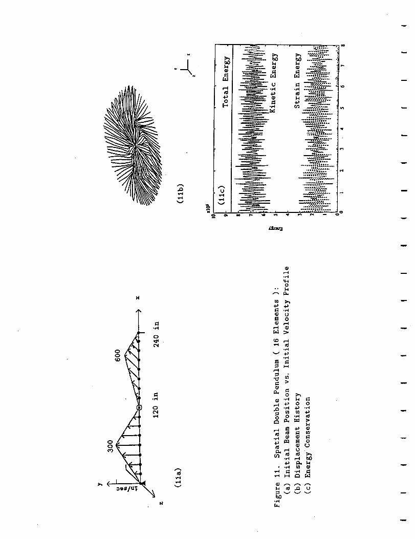
dynamics framework, the final example of a spatial double pendulum is given. The double

pendulum is modeled with two beams; a spherical joint connects the last node of the first

beam to the first node of the second beam and also pins the first node of the first beam.

It is noted that the joint connection can easily be accounted for from a finite element

assemblage which leaves the rotational degrees of freedom free at the hinge location. The

method was used to verify the results obtained using the Lagrange multiplier solver on the

augmented equations described in Section 3.5. In the first case, the pendulum is subjected

to a gravity field in the vertical z-direction and an initial velocity impulse in the horizontal

x-y plane such that soley rigid motion is

increasing beam flexibility as follows:

1. EA = 1.0 x 104 Ib

2. EA = 1.0 x 103 lb

3. EA = 2.0 x 102 Ib

4. EA = 1.0 x 102 lb

with the remaining parameters

excited. The problem is run for four cases of

GA = 0.5 x 104 lb"

GA =O.5 x 103 Ib

GA = I.O x 102 Ib

GA =O.5 x 102 Ib

26

pA = 1 Ibm�in pI = .833 x 10 -s Ibm in l = 1 in

held constant. The initial velocity impulse, and the spatial trajectories of the mass

center of the second beam as projected on the x-y and x-z planes is given in Figure 9. The

trajectory of the first case coincides exactly with a rigid body solution to the problem,

and the slight deviation of the trajectories due to the increasing flexibility can be seen.

The energy time histories for the problem, given in Figure 10, verify the computational

objectivity of the algorithm as again energy is identically conserved. Again, the invariance

of the internal force calculations in the three dimensional environment is witnessed by the

negligible strain energy contribution for all of the flexible cases. The time integration of

the spatial kinematics preserves the balance between the kinetic and potential energies of

the problem. Next, the flexible double pendulum is given an initial velocity impulse to

excite deformation motion as well as the rigid motion. For this case the parameters used

were

EA = 1.8 x 108 lb, GA = 0.9 x 10 s lb, EI = 1.4 x 10 s lb in 2

pA =.98Ibm�in, pI = 0.67 Ibm in, l = 120 in.

The initial velocity profile, the resulting time histories of several deformed configurations

and energy time history are given in Figure 11, exhibiting the large spatial rotation and

deformation capabilities of the formulation. The energy conservation is retained for the

computations of spatial deformations.

Further examples of large scale multibody systems are in process, and these results

axe to be presented in the near future.

7. Concluding Remarks

A flexible beam finite element that is readily incorporated into multibody dynamics

applications has been presented. The beam formulation is based on fully nonlinear strain

measures which remain invariant to rigid body motions. The model retains a Cauchy

stress and physical strain description, and as such it can be easily interfaced with real-

time slewing control applications as the measured strains can directly be used as a feedback

signal without requiring sophisticated transformations. In addition, the formulation uses

an inertial reference for the beam dynamics such that the degrees of freedom of the flexible

component are defined in the same sense as the rigid components by including without dis-

tinction both the rigid and flexible deformation motions. The consequence is adaptability

into multibody dynamics methodologies as numerical solution procedures for the integra-

tion of spatial kinematic systems can directly be applied to the generalized coordinates of

both the rigid and flexible components. The success of the approach relies on an accurate.

computation of the nonlinear internal force term. For this reason, the calculation of finite

strain increments has been presented which axe invariant to arbitrary rigid motions of the

beam. The proposed methodology is suitable to treat the dynamics of flexible beams which

27

undergo a variety of structural deformations in addition to the large overall motions. Thesameapproach can be used in formulating other types of structural components.

Acknowledgements

The work reported herein was supported by .NASA/Langley Research Center under

Grant NAG-I-756. The authors wish to thank Dr. Jerry Housner for his interest and

support during the course of the present work.

8. References

1. Ashley, H., "Observation on the dynamic behavior of flexible bodies in orbit," AIAA

J. 5 (1967), 460-469

2. Canavin, J.R. and Likins, P.W., "Floating reference frames for flexible spacecraft," J.

of Spacecraft (1977), 724-732.

3. De Veubeke, B.F., "The dynamics of flexible bodies," Int J. Engng. Sci. 14 (1976),

895-913.

4. Grotte, P.B., J.C. McMunn, and R. Gluck, "Equations of motion of flexible space-

craft," d. of Spacecraft and RockeU 8 (1971), 561-567.

5. McDonough, T.B., "Formulation of the global equations of motion of a deformable

body," AIAA ]. 14 (1976), 656-660.

6. Kane, T. and Levinson, D., "Simulation of large motions of nonuniform beams in orbit:

Part II - The unrestrained beam," J. Astronautical Science8 29, (1981), 245-275.

7. Bodley, C., Devers, A., Park, A., and Frisch, H., "A digital computer program for dy-

namic interaction simulation of controls and structures (DISCOS)," NASA Technical

Paper 1219, May 1978.

8. Song, J.O. and Haug, E.J., "Dynamic analysis of planar flexible mechanisms," Comp.

Meth. Appl. Mech. Engrg. 24 (1980), 359-381.

9. Cavin, R.K. and Dusto, A.R., "Hamilton's principle: finite-element methods and

flexible body dynamics," AIAA J. 15 (1977) 1684-1690.

10. Agrawal, O.P. and Shabana, A.A., "Dynamic analysis of multibody systems using

component modes," Computers _ Structures 21 (1985), 1303-1312.

11. Agrawal, O.P. and Shabana, A.A., "Application of deformable-body mean axis to

flexible multibody system dynamics, " Comp. Meth. Appl. Mech. Engrg. 56 (1986),217-245.

12. Shabana, A.A. and Wehage, R.A., "A coordinate reduction technique for dynamic

analysis of spatial substructures with large angular rotations," J. Slruct. Mech. 11

(1983), 401-431.

28

13. Yoo, W.S. and Haug, E.J., "Dynamics of articulated structures, Part I: Theory andPart II: Computer implementation and applications," J. of Structure Mechanics 14

(1986), 105-126 and 177-189.

14. Yoo, W.S. and Haug, E.J., "Dynamics of flexible mechanical systems using vibra-

tion and static correction modes," J. Mechanisms, Transmissions, and Automation in

Design 108 (1986) 315-322.

15. Belytschko, T. and Hsieh, B.J., "Nonlinear transient finite element analysis with con-

vetted coordinates," Int. J. Num. Meth. Eng. 7 (1973), 255-271.

16. Belytschko, T., Schwer, L., and Klein, M.J., "Large displacement, transient analysis

of space frames," Int. J. Num. Meth. Eng. 11 (1977), 65-84.

17. Housner, J., "Convected transient analysis for large space structures maneuver and

deployment," Proe. the 25th Structures, Structural Dynamics and Materials Confer-

ence, AIAA Paper No. 84-1023, (1984) 616-629.

18. Housner, J.M., Wu, S.C., and Chang, C.W., "A finite element method for time varying

geometry in multibody structures," Proc. the 29th Structures, Structural Dynamics

and Materials Conference, April 1988, AIAA Paper No. 88-2234.

19. Laskin, R.A., Likins, P.W., and Longman, R.W., " Dynamical Equations of a Free-

Free Beam Subject to Large Overall Motions," J. Astronautical Sciences 31 (1983),

507-528.

20. Kane, T.R., Ryan, R.R., and Banerjee, A.K., "Dynamics of a cantilever beam attached

to a moving base," J. Guidance, Control, and Dynamics 10 (1987) 139-151.

21. Wu, S.C. and Haug, E.J., "Geometric nonlinear substructuring for dynamics of flexible

mechasfical systems," Int. J. Num. Meth. Engrg. 26 (1988)2211-2226.

22. Bakr, E.M. and Shabana, A.A., "Geometrically nonlinear analysis of multibody sys-

tems," Computers _ Structures 23 (1986) 739-751.

23. Christensen, E.R. and Lee, S.W., "Nonlinear finite element modeling of the dynamics

of unrestrained flexible structures," Computers _ Structures 23 (1986) 819-829.

24. Cardona, A. and Geradin, M., "A beam finite element nonlinear theory with finite

rotations," Int. J. Num. Meth. Eng. 26 (1988), 2403-2438.

25. Iura, M. and Atluri, S.N., "On a consistent theory, and variational formulation of

finitely stretched and rotated 3-D space-curved beams," Computational Mechanics

(4) (1989), 73-88.

26. Simo, J.C., "A finite strain beam formulation. Part I: The three dimensional dynamic

problem," Comp. Meth. Appl. Mech. Engrg. 49 (1985), 55-70.

27. Simo, J.C. and Vu-Quoc, L., "A three-dimensional finite strain rod model. Part II:

Computational aspects," Comp. Meth. Appl. Mech. Engrg. 58 (1986), 79-116.

28. Simo, J.C. and Vu-Quoc, L., "Finite-strain rods undergoing large motions," Comp.

Meth. Appl. Mech. Engrg. 66 (1988), 125-161.

29

29. Antman, S.S., "Kirchhoff problem for nonlinearly elastic rods," Quat. J. Appl. Math

XXXII 3 (1974), 221-240.

30. Reissner, E., "On a one-dimensional large-displacement finite-strain beam theory,"

Studies in Applied Mathematics 52 (1973), 87-95.

31. Reissner, E., "On finite deformations of space--curved beams," ZAMP 132 (1981),734-744.

32. Wempner, G., Mechanics of Solids with Applications to Ttu'n Bodies, Sijthoff & No-

ordhoff, The Netherlands (1981).

33. Goldstein, H., Classical Mechanics, 2nd ed., Addison-Wesley (1980).

34. Malvern, L.E., Introduction to the Mechanics of a Continuous Medium, Prentice-Hall,

Inc., Englewood Cliffs, N. J., (1969).

35. Eringen, A.C., Mechanics of Continua, Robert E. Krieger Publishing Co., Huntington,

N.Y., (1980).

36. Zienkiewicz, O.C., 1977, The Finite Element Method, 3rd ed., McGraw Hill Book

Company, Ltd, London.

37. Lanczos, L., The Vaxiational Principles of Mechanics, 4th ed., University of Toronto

Press, 1970.

38. Park, K.C., and Chiou, J.C., "Evaluation of constraint stabilization procedures for

multibody dynamical systems," Proc. the 28th Structures, StructurM Dynamics and

Materials Conference, Part 2A, Monterey, CA, AIAA Paper No. 87-0927 (1987),769-773.

39. Park, K.C., and Chiou, J.C., "Stabilization of computational procedures for con-

strained dynamical systems," Journal of Guidance, Control and Dynamics 11 (1988),365-370.

40. Park, K.C., Chiou, J.C., and Downer, J.D., "A computational procedure for large

rotational motions in multibody dynamics," Proc. the 29th Structures, Structural

Dynamics and _laterials Conference, Part 3, Williamsburg, VA, AIAA Paper No.

88-2416 (1988), 1593-1601 (also to appear in J. Guidance, Control and Dynamics).

41. Park, K.C., Chiou, J.C., and Downer, J.D., "An explicit-implicit staggered procedure

for multibody dynamics analysis, Part I: Algorithmic aspects," Report No. CU-CSSC-

88-08, Center for Space Structures and Controls, University of Colorado (1988).

42. Wittenburg, J., Dynamics of Systems of Rigid Bodies, B.G. Teubner, Stuttgart, 1977.

43. Rankin, C.C. and Brogran, F.A., "An element independent corotational procedure

for the treatment of large rotations," J. of Pressure Vessel Technology 108 (1986)165-174.

44. Geradin, M., Robert, G., and Buchet, P.,"Kinematic and dynamic analysis of mecha-

nisms: A finite element approach based on Euler parameters," in: Finite Element

Methods for Nonlinear Problems(P. Bergan, ed.), Berlin, Heidelberg, New York,

Springer, 1986.

3O

FIGURES

b2bl

r

Figure I. Beam Kinematics

X> e,

e2

Je3

!

el

Figure 2. Convected Reference Frame

s,_ "

Figure 3. Pure Bending of Beam Element

0..4

4_U

@

-m,-¢

(-.

0.7

0.6

0.5

0.4

0.3

0.2

0.1

0.0

0.0

I I i ! ! I I I I

6.0 12.0 18.0 24.0 30.0

Time ( sec )

(4b)

Figure 4. Geometric Stiffening ( 5 Elements )'

(a) Tip Deflection vs. Time

(b) Displacement History

i

600

U@I0

I=

1

200 in

(Sa)

X

t = 1.15 sec

(Sb) L,

t = .01 sec

t = 2.30 sec

Figure 5. First Bending Mode ( 8 Elements ):

(a) Initial Beam Position vs. Initial Velocity Profile

(b) Displacement History

300

U

-300

(6a)

: X

(6b)

f

I

= 14.0 sec

t = .I see

Figure 6. Second Bending Mode ( 12 Elements ):

(a) Initial Beam Position vs. Initial Velocity Profile

(b) Displacement History

Y

4so t_

_ H y

200 in

-450

(Ta)

Figure 7. Combination Bending Mode ( 16 Elements ):

(a) Initial Beam Position vs. Initial Velocity Profile

(b) Displacement History

w

,ed

,-4

CDw-4

X

bO

_4

0_

-0.50

• , T°talEnergyI

%; -.y,,:-;"i'/_/'_/'.,[",../.j,,",,:'....:",,'".....--/

Kinetic Energy

Strain Energy

' " .' " : : :: I : : " :: $: ;: * : " • ,': " " "" :: :: ::

Time (sec)

Figure 8. First Bending Mode: Energy Conservation

1

1.5

I

0.5

0

-I

-1.5

*2-2

(9a)

-_ _ o15 _ I_

hl

2

1.5

1

0.5

0

-0.5

-i

-1.5

-2-2

(9b)

/.5 .', -o'_ _ o15 i ,'._

Figure 9. Spatial Double Pendulum ( 16 Elements ):

(a) Second Beam Trajectory: X-Y Plane

• (b) Second Beam Trajectory: X-Z Plane

% ..

F,.,-I .,, ., l..,.1

<2

...o...... ..._....o...o _......

_.°" ....)

I I r'_'' | ""..i i I

crl

N

qf

"0

(_ ql) '_l_:"u':!

_... "._.

• _1 _:._

I

I

L

IT

"°,..,_ i,..,. _'''°'''''¸¸'_

• _-' ,.°.°

[.,..I ('_ /' I.,-I

s. o" ".,_

°*'*°*'%,.... _...._ ........

,_J '"-., _.# 'I.,- ......... ._

• ......._, ...... .. (.

*_.,,.,___

.,.j

.._ ........ _!

"s'_"* "% "_i'

"-L.'"..........'.:.':.':.-':".':i............... _:.i...

i I I" I "i I I 1

.. _ o0

o

oo

ll_ I I I"" I *" I

' ' ....'...>:'.::L.I.......'

,'..................7 r..,a 'I

'........ ,

_.':,. ..............1 _;ii

f.. ..... "I

_, °. ,,

......."" ""._."-,L...........

•."" "\ :1'

k / .

.,....::"<............. ._°r°.* .............. . ¢_!

.... ! 1

..........;.:,_-_:'._............ ii

i I

o

(u! ql) X_J_U"_

c,

,o

I--

_0

o

o

o

XXX×

_ II II II [l

•_ X X X X

II II H 11

.__

M

N

[ •

1::8

a"-'4

0F'*

U

O

o

0

v

o°°

QJ Uo

,-4r_ _J

_D r_

°_

0

r-I _ 0 0,._ ._ _ .,-a

_ El o

• ,..4 ,-4

• .el _

,,,-,0 _-0 _ _a,.1

_ ._ u

_0