Purdue UniversityPurdue e-Pubs

CTRC Research Publications Cooling Technologies Research Center

2011

A comprehensive model of a miniature-scale linearcompressor for electronics coolingCraig R. BradshawPurdue University - Main Campus

Eckhard A. GrollPurdue University - Main Campus

S V. GarimellaPurdue University, sureshg@purdue.edu

Follow this and additional works at: https://docs.lib.purdue.edu/coolingpubs

This document has been made available through Purdue e-Pubs, a service of the Purdue University Libraries. Please contact epubs@purdue.edu foradditional information.

Bradshaw, Craig R.; Groll, Eckhard A.; and Garimella, S V., "A comprehensive model of a miniature-scale linear compressor forelectronics cooling" (2011). CTRC Research Publications. Paper 147.http://dx.doi.org/doi:10.1016/j.ijrefrig.2010.09.016

A Comprehensive Model of a Miniature-Scale Linear

Compressor for Electronics Cooling

Craig R. Bradshawa,b,1, Eckhard A. Grolla,b, Suresh V. Garimellab

aHerrick Laboratories, Purdue University, West Lafayette, IN 47907

bCooling Technologies Research Center, Purdue University, West Lafayette, IN 47907

Abstract

A comprehensive model of a miniature-scale linear compressor for electronics cooling is

presented. Linear compressors are appealing for refrigeration applications in electronics cooling.

A small number of moving components translates to less theoretical frictional losses and the

possibility that this technology could scale to smaller physical sizes better than conventional

compressors. The model developed here incorporates all of the major components of the linear

compressor including dynamics associated with the piston motion. The results of the compressor

model were validated using experimental data from a prototype linear compressor. The prototype

compressor has an overall displacement of approximately 3cm3, an average stroke of 0.6 cm. The

prototype compressor was custom built for this work and utilizes custom parts with the exception

of the mechanical springs and the linear motor. The model results showed good agreement when

validated against the experimental results. The piston stroke is predicted within 1.3% MAE. The

volumetric and overall isentropic efficiencies are predicted within 24% and 31%, MAE

respectively.

Keywords: linear compressor, compressor model, electronics cooling, miniature compressor

_____________________________________________________________________________

Nomenclature

A

area [m2]

CD

drag coefficient for flow past reed valve [-]

Cv

specific heat capacity at constant volume [Jkg-1K-1]

D

diameter [m]

E

total energy in the control volume [kW]

Fdrive

driving force from linear motor [N]

JCG

rotational moment of inertia for the piston about the CG [kgm]

M

moving mass [kg]

MAE

Mean absolute error [-]

P

pressure of gas [kPa]

Phigh

higher pressure [kPa]

Plow

lower pressure [kPa]

Ramb

thermal resistance between the compressor shell and ambient [WK-1]

Re

Reynolds number[-]

T

temperature of gas[K]

V

volume of control volume [m3]

W

work [J]

total heat transfer into the control volume [kW]

Ẇ

total work on the control volume [kW]

ṁ

mass flow rate [kgs-1]

V

gas velocity [ms-1]

f

dry friction coefficient between piston and cylinder [-]

k

thermal conductivity[Wm-1K-1]

ceff

effective damping of piston [Nsm-1]

f

resonant frequency of piston operation [Hz]

g

leakage gap width [m]

h

specific enthalpy [kJkg-1]

k

stiffness or spring rate [Nm-1]

q

heat flux[Wm-2]

t

time [sec]

u

internal energy [kJkg-1]

v

specific volume of gas [m3kg-1]

x

displacement [m]

Greek letter

α

thermal diffusivity[m2s-1]

ϵ

eccentricity of spring force [m]

η

efficiency [-]

γ

heat capacity ratio[-]

ωd

damped natural frequency[radsec-1]

ρ

density of gas [kgm-3]

θ

rotational angle of piston [rad]

Subscripts

amb

ambient

cv

control volume

discharge

gas discharged from compression chamber

exp

experimental value

gas

quantity resulting from gas

in

into control volume

leak

leakage

mech

mechanical

o,is

overall isentropic

out

out of control volume

p

piston

port

valve port opening

shell

compressor shell

suction

suction gas

tr

transitional

v

constant volume process

valve

reed valve

vol

volumetric

1. Introduction

Miniature refrigeration systems offer distinct advantages for use in electronics cooling relative to

other technologies. Only refrigeration offers the ability to cool components below the ambient

temperature. The reliability and performance of semi-conductor devices is improved when

operating at lower temperatures. Because vapor compression utilizes two-phase heat transfer in

the evaporator, it is possible to maintain spatially uniform chip temperatures. The major concerns

involving refrigeration systems are their cost and reliability, as well as miniaturization of the

different components.

Trutassanawin et al. (2006) reviewed the available technologies for vapor compression

systems in electronics cooling. Several prototype systems were discussed but there appeared to

be no commercially viable solutions which are complete miniature systems. Chiriac and

Chiriac (2008) concurred with this assessment in a recent review. Other investigations into

refrigeration technology have led to the development of system prototypes (Mongia et al., 2006)

and system-level models such as ones by Heydari (2002) and Possamai et al. (2008). However, it

has been reported that the overall performance and size of these systems is still not at a level that

is desired for desktop and portable electronic systems (Cremaschi et al., 2007). In particular the

compressor is a critical component which can greatly affect the overall size and performance of

the refrigeration system, as shown by Trutassanawin et al. (2006).

In electronics cooling applications, an atypical challenge for refrigeration systems is the

relatively small temperature lift for cycle operation. The temperature lift is limited on the high-

side by the environmental conditions and on the low-side by the desire to eliminate possible

water vapor condensation from the ambient within the electronic package. Typically, this leads

to a system with a small pressure ratio, as shown in Figure 1, which displays a typical

refrigeration cycle for electronics cooling using R-134a as the working fluid. The small pressure

ratio leads to poor performance for currently available small-scale compressors, which are

designed for refrigerator applications with a significantly larger pressure ratio. Some past studies

using currently available technology have operated the compressors at a larger pressure ratio, and

instead, developed solutions to handle moisture condensation by operating the evaporator and

chip assembly in heavily insulated volumes (Heydari, 2002). The disadvantage of this option is a

further increase in the cost of the cooling system.

A linear compressor is appealing for electronics cooling applications because it offers several

potential advantages over traditional compressor technology. A linear compressor is a positive

displacement compressor, similar to a reciprocating compressor. However, a linear compressor

does not have a crank mechanism to drive the piston. Instead the piston is driven directly by a

linear motor, as seen in Figure 2. The omission of the crank mechanism significantly reduces the

frictional losses associated with conventional reciprocating compressors. It also allows oil-free

operation which is a significant advantage with respect to the heat transfer performance of the

condenser and evaporator in the system.

In addition, a linear compressor is designed as a resonantly operated device. This means that

mechanical springs are used to tune the device to operate at a resonant frequency. Operation at a

resonant frequency allows a desirable reduction in size of the motor.

Early investigations of a linear compressor were conducted by Cadman and Cohen (1969a,b)

for traditional refrigeration systems. Cadman and Cohen observed that the free piston operation

of this device created some peculiar effects such as piston drift, which posed a challenge to

modeling efforts and limited the practical application such devices. Pollak et al. (1979)

investigated one-dimensional, nonlinear dynamics of the piston and electrical systems and

confirmed such confounding effects.

Van der Walt and Unger (1994) assessed the state of the art in linear compressor technology.

Unger and Novotny (2002) and Unger (1998) developed several linear compressor prototypes

and performed a feasibility study which showed the potential for linear compressors in cryogenic

and miniature systems. There have also been studies on the unique differences in the

performance of linear compressors compared to conventional reciprocating compressors (Lee

et al., 2001, 2004). Recently, Possamai et al. (2008) developed a prototype refrigeration system

for a laptop cooling application which utilized a linear compressor. Another recent study on

linear compressors investigated the sensitivity of the device to changes in operating frequency

(Kim et al., 2009). This study utilized a single degree of freedom vibration model coupled to an

electrodynamic motor model as was done by Pollak et al. (1979).

Past models of linear compressors have often employed linearizing assumptions or were

restricted to a single degree of freedom in their analysis. Such analyses have either used a greatly

simplified representation of device operation or have focused on specific components of the

overall system. The present work develops a comprehensive compressor model which

incorporates all of the major dynamics and nonlinearities as well as a second degree of freedom

in the piston motion. In addition, the model predictions are validated using experimental data

from a prototype linear compressor.

2. Model Formulation

The major components of the linear compressor model are described in this section. The

comprehensive compressor model consists of a solution to two compression process equations

that provide the temperature and density, and thus fix the state within each control volume.

These equations require inputs from the five sub-models representing the valve flows, leakage

flows, motor losses, heat transfer from the cylinder, and piston dynamics. The compression cycle

is discretized and an initial guess of temperature and density is made within each control volume.

The compression process equations are then used to step through a compression cycle using the

numerical techniques described in Section 2.7. Comprehensive compressor models of this nature

have been developed for other compressor types (Chen et al., 2002a,b, Kim and

Groll, 2007, Mathison et al., 2008).

2.1. Compression Process Equations

The compression process is modeled using mass and energy conservation over a control volume.

In order to determine the state of the working fluid in the compression chamber at any point

during the compression process, it is necessary to determine two independent fluid properties to

fix its state. In this analysis the compressor is split into two control volumes as illustrated in

Figure 2. The first is the compression chamber for the compressor, while the second consists of

the remaining volume within the compressor. The compression process equations are solved for

each control volume at a particular time step and coupled through the leakage, vibration, and

heat transfer sub-models.

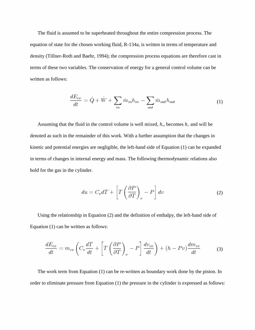
The fluid is assumed to be superheated throughout the entire compression process. The

equation of state for the chosen working fluid, R-134a, is written in terms of temperature and

density (Tillner-Roth and Baehr, 1994); the compression process equations are therefore cast in

terms of these two variables. The conservation of energy for a general control volume can be

written as follows:

(1)

Assuming that the fluid in the control volume is well mixed, hout becomes hcv and will be

denoted as such in the remainder of this work. With a further assumption that the changes in

kinetic and potential energies are negligible, the left-hand side of Equation (1) can be expanded

in terms of changes in internal energy and mass. The following thermodynamic relations also

hold for the gas in the cylinder.

(2)

Using the relationship in Equation (2) and the definition of enthalpy, the left-hand side of

Equation (1) can be written as follows:

(3)

The work term from Equation (1) can be re-written as boundary work done by the piston. In

order to eliminate pressure from Equation (1) the pressure in the cylinder is expressed as follows:

(4)

By combining these relations:

(5

)

in which only temperature is the independent variable. The other independent fluid property is

density, which is computed as:

(6)

The change in mass in the cylinder can then be written as:

(7)

Equations (5) - (7) can now be solved simultaneously for the temperature and density in the

two control volumes. Due to the nonlinear nature of these equations, a numerical solution

approach is adopted. A number of inputs to this solution must still be determined from various

sub-models as will be discussed below.

2.2. Valve Model

Reed valves are used in the present work as is typical for reciprocating compressors. These

valves are essentially cantilevered beams which are displaced when a differential pressure is

imposed across them. To ensure that pumping, as opposed to back flow, of the gas occurs, two

valves are used with limited ranges of operation. The valve body is constructed to only allow

valve motion in the direction of desired flow for each valve; this ensures that pumping occurs

and can be seen in Figure 3.

Valve analysis is split into two modes of operation depending on the location of the valve

reed, similar to the analysis of Kim and Groll (2007). Early in its deflection the stagnation

pressure driving the valve reed is assumed equal to the high side pressure. As the valve opens

further, this assumption becomes less valid, as the movement of the valve is now dominated by

the movement of fluid past the valve and the stagnation pressure becomes equal to the low-side

pressure. These two modes of operation are referred to as the pressure-dominant and mass-flux-

dominant modes, respectively, with free-body diagrams as shown in Figure 4. The port area is a

fixed quantity and represents the opening that fluid travels through in the valve body. The valve

area is an effective area, taken as a circular area based on the width of each valve reed.

For each mode of operation an equation can be written based on the free-body diagrams

shown in Figure 4. Summing the forces in the direction of displacement, the equation of motion

for the pressure-dominated and mass flux-dominated modes may be expressed as:

(8

)

(9

)

These second-order, nonlinear equations can be solved for the position of the reeds at each

time step throughout the compression process. The valve geometry, shown in Figure 3, can be

used to determine the required valve and port areas and the density is calculated from the

compression process equations. The gas velocity is calculated assuming an isentropic,

compressible flow across the valve. The mass and stiffness of the reeds can be calculated by

assuming that each reed behaves as an Euler beam. The stiffness is calculated by dividing an

arbitrary applied force by the deflection it produces. The effective mass is then found by dividing

the total valve mass by a factor of three, as in the case of the effective mass of a spring

(Rao, 2004).

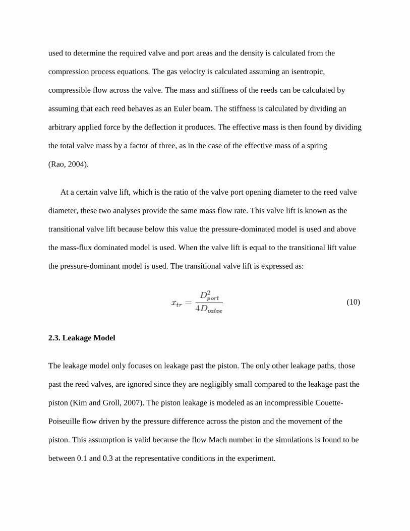
At a certain valve lift, which is the ratio of the valve port opening diameter to the reed valve

diameter, these two analyses provide the same mass flow rate. This valve lift is known as the

transitional valve lift because below this value the pressure-dominated model is used and above

the mass-flux dominated model is used. When the valve lift is equal to the transitional lift value

the pressure-dominant model is used. The transitional valve lift is expressed as:

(10)

2.3. Leakage Model

The leakage model only focuses on leakage past the piston. The only other leakage paths, those

past the reed valves, are ignored since they are negligibly small compared to the leakage past the

piston (Kim and Groll, 2007). The piston leakage is modeled as an incompressible Couette-

Poiseuille flow driven by the pressure difference across the piston and the movement of the

piston. This assumption is valid because the flow Mach number in the simulations is found to be

between 0.1 and 0.3 at the representative conditions in the experiment.

The leakage mass flow rate is calculated using the average leakage velocity obtained by

integrating the velocity profile as:

(11)

2.4. Heat Transfer Model

The instantaneous heat transfer from each of the control volumes is calculated using the

empirical approach of Fagotti and Prata (1998).

(12)

where:

(13)

By integrating these instantaneous heat transfer rates over the entire cycle, the total heat

transfer from each of the two control volumes is calculated for use in the overall energy balance.

2.5. Vibration Model

A linear compressor is a free-piston device for which the stroke is not fixed by a crank

mechanism but is instead determined by chosen geometry, the linear motor, and the mechanical

springs used. The piston dynamics are modeled using a free body diagram of the piston assembly

as shown in Figure 5.

Both the desired linear motion of the piston as well as its undesirable rotation due to

eccentricity in the mechanical springs are considered. Any eccentricity causes a perpendicular

reactionary load from the mechanical spring as it is compressed, since the spring cannot react to

a load along its entire circumference. Thus, the effective load acts at a point offset from the

center of mass of the piston. In a traditional compression spring as used in the prototype

fabricated for this work, this point is assumed to be along the circumference of the spring where

the edge of the spring contacts the piston assembly.

The linear motion of the piston as well as its rotation, are modeled as a two-degree of

freedom vibration system. By assuming that the piston is a rigid body and the motions in the y

and z directions as well as the rotation are small, the following equations describe the motion of

the piston:

(14)

(15)

In addition, it is assumed that the driving force and the reactionary forces from the

compression chamber are applied directly through the center of mass of the piston.

The driving force, Fdrive, is the sinusoidal force applied from the motor. The power transmitted

to the piston is calculated by assuming an efficiency for the motor. The stiffness associated with

the gas, kgas, is determined by linearizing the force generated by the gas over an entire

compression cycle. This gas force is then divided by the stroke of the compressor which yields

an effective spring rate of the gas in the compression chamber.

(16)

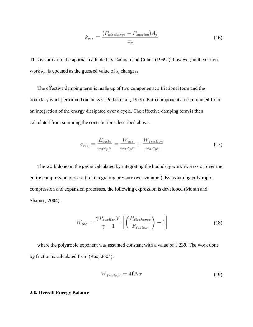
This is similar to the approach adopted by Cadman and Cohen (1969a); however, in the current

work kgas is updated as the guessed value of xp changes.

The effective damping term is made up of two components: a frictional term and the

boundary work performed on the gas (Pollak et al., 1979). Both components are computed from

an integration of the energy dissipated over a cycle. The effective damping term is then

calculated from summing the contributions described above.

(17)

The work done on the gas is calculated by integrating the boundary work expression over the

entire compression process (i.e. integrating pressure over volume ). By assuming polytropic

compression and expansion processes, the following expression is developed (Moran and

Shapiro, 2004).

(18)

where the polytropic exponent was assumed constant with a value of 1.239. The work done

by friction is calculated from (Rao, 2004).

(19)

2.6. Overall Energy Balance

To ensure that all of the compressor components satisfy an energy balance, a thermal network is

constructed to account for heat transfer from the compression chamber (Chen et al., 2002a, Kim

and Groll, 2007, Mathison et al., 2008). The energy balance for the compressor assumes that the

heat transfer between the two control volumes is negligible and that the heat only flows to the

compressor shell. A lumped-mass thermal network can then be constructed consisting of a single

lumped mass to represent the compressor shell with two heat inputs and one heat output to the

ambient. The heat output path is calculated using a forced convection correlation for flow over a

cylinder to determine the thermal resistance between the compressor shell and the ambient

(Hilpert, 1933). The thermal network elements are also shown in Figure 2. This network adds the

following relation which is solved simultaneously with the compression process equations.

(20)

2.7. Solution Approach

The model developed above for the linear compressor consists of two non-linear first-order

differential equations for the compression process and one non-linear equation from the energy

balance. An explicit closed-form solution is not available, and the equations are instead solved

numerically. The compression process is discretized into small time steps and each equation is

solved using a fourth-order Runge-Kutta method.

The order in which the model steps through the series of equations is shown in Figure 6. The

key input guesses to the model are the compressor inlet pressure and temperature, and the desired

discharge pressure. For each time step, the model sequentially steps through each sub-model and

calculates the solution inputs for the next time step. Once each sub-model has been called the

overall compression process solver is called which solves Equations (5) to (7) and calculates the

internal state in the compressor. When the model has iterated through an entire compression

cycle Equation (20) is solved for Tshell. When the changes in temperature and density in each of

the two control volumes as well as the change in Tshell is less than 0.01%, a converged solution is

available. The initial conditions in both control volumes were set to the inlet conditions for each

operating condition that was tested. The number of iterations required for convergence varied

between approximately 20 and 150 depending on operating conditions.

3. Experiments

No linear compressors are commercially available in the capacity and pressure ranges desired for

electronics cooling. Therefore, a prototype compressor was custom-designed and built for the

purpose of conducting experiments that could serve to validate the model developed in this work.

The compressor was built using a moving-magnet type linear motor (H2W Tech). The housings,

piston, and valve assembly were built in-house. A cross-sectional view of the prototype

compressor is shown in Figure 7, with key dimensions given in Table 1.

The prototype linear compressor was tested on a compressor load stand specifically built for

testing miniature-scale compressors. The compressor load stand is based on a hot-gas bypass

design; a schematic is shown in Figure 8. This type of load stand has been used successfully in

previous studies to conduct performance tests compressors (Sathe et al., 2008, Hubacher

et al., 2002). The load stand cycle state points are shown in a pressure enthalpy diagram in

Figure 9. The compressor operates between state points 1 and 2. From state point 2, the gas is

expanded across a set of valves to an intermediate pressure at state point 3. The flow from state

point 3 is divided into two flow paths. One path runs through the condenser and is cooled to a

saturated liquid at state point 4. It is then isenthalpically expanded to the compressor suction

pressure at state point 5. The hot-gas bypass flow is expanded from the intermediate pressure to

the compressor suction pressure at state point 6. The flows at state points 5 and 6 are mixed to

provide the compressor suction state at state point 1. By controlling the ratio of these two flows

the inlet pressure and temperature can be controlled. The discharge pressure of the compressor is

controlled by adjusting the valve between state points 2 and 3.

The compressor was tested under a range of operating conditions, which simulate an

electronics cooling application. At each specific set of compressor inlet conditions, the

compressor was operated until a steady state condition was achieved, at which point data was

collected. This process was then repeated for subsequent compressor inlet conditions which are

tabulated in Table 2. It is noted that the performance testing of a linear compressor is

significantly different from that of conventional positive displacement compressors. During the

performance testing of conventional compressors, the stroke and frequency of the piston are

naturally held constant due to the kinematics of the device. However, a linear compressor

requires that the frequency be adjusted to maintain operation at resonance. The power input and

operating frequency are varied in these tests so as to maintain similar stroke values throughout

the testing. The state points achieved in the experiments are summarized in Table 2.

The volumetric efficiency shown in Table 2 is defined as follows:

(21)

This definition accounts for volumetric losses as well as a dependence on the piston dynamics.

The overall isentropic efficiency of the device, also listed in Table 2, is defined as follows:

(22)

This definition accounts for all the losses, and as a result, is used as an overall benchmark for

compressor performance.

3.1. Experimental Uncertainty

A variety of measurements were obtained in the experiments including temperature and pressure

at the suction and discharge ports, mass flow rate of refrigerant, piston stroke, frequency, and

input power. The measurements of pressure, temperature, and stroke have absolute uncertainties

of 4.6 kPa, 0.5 C, and 25.40 μm, respectively. The Coriolis mass flow meter has relative absolute

uncertainty values between 0.350 and 1.25 %, depending on the quantity of mass flow measured.

The frequency and input power have absolute uncertainty values which varied from 2.07 x 10-4 to

5.10 x 10-4Hz and 0.188 and 0.532 W, respectively which are calculated using a 99.95%

confidence interval. The uncertainty in the reported efficiency values is calculated using an

uncertainty propagation analysis (Fox et al., 2004). The volumetric and overall isentropic

efficiencies have absolute uncertainty value ranges of 1.07 x 10-3 to 2.29 x 10-3 and 1.05 x 10-3 to

1.90 x 10-3, respectively.

4. Validation of Model Predictions

The experimental results are compared to the predictions from the model. The model

performance is quite sensitive to several parameters: the leakage gap between the piston and

cylinder, g, the eccentricity of the piston, ϵ, the dry friction coefficient, f, and the linear motor

efficiency, ηmotor. Since these parameters are difficult to measure, best estimates were used and

adjusted within reasonable ranges to provide the best fit with the experimental data. The leakage

gap was chosen based on the design dimensions to be in the range of 0.1 to 0.4mm. The initial

guess of eccentricity was set to the radius of the compression spring used in the prototype

compressor, this value varied between 9.2 to 11.4mm. The dry friction coefficient was varied

between 0.2 and 0.4. The motor efficiency was estimated based on the measured heat loss from

the prototype compressor and was varied between 40% and 50%. These parameter values are

summarized in Table 1.

The parameters in Table 1 along with experimental values for the suction and discharge

pressure, suction temperature, frequency, and input power (Table 2) were used as inputs to the

model. Figures 10 to 13 show the major model predictions compared with the experimental

results for piston stroke, mass flow rate, volumetric efficiency, and overall isentropic efficiency,

respectively. The model predicts the stroke of the linear compressor within 1.3% MAE as shown

in Figure 10. The predicted mass flow rates are shown in Figure 11 and agree with the measured

values to within 20% MAE. The predicted volumetric efficiency shows a similar behavior to the

mass flow rate, predicting the experimental results to within 24% MAE, as shown in Figure 12.

In the performance testing of conventional compressors the volumetric efficiency is simply a

dimensionless mass flow rate. However, for a linear compressor, the volumetric efficiency

depends not only on the mass flow rate but also the frequency, as seen in Equation (21). The

piston stroke also varies slightly depending on the operating condition, which affects the

volumetric efficiency. The overall isentropic efficiency is predicted by the model to within

roughly 31% MAE as shown in Figure 13. MAE, mean absolute error, is defined as the average

of the absolute value of errors.

The overall isentropic efficiency of the prototype compressor is significantly lower than for

typical commercially available compressors. However, the purpose of the prototype built in this

work was merely to validate the model and not to obtain optimized performance. Since no

commercial prototype was available which could be tested for this work, the compressor was

made in-house, and could admittedly be significantly improved. However, the operating

principles underlying the model and the prototype are identical, and therefore, the experiments

serve the purpose of validating model predictions. It is expected that the model can form the

basis for more optimized prototypes to be designed. The model developed in this work can be

applied in the analysis of any linear compressor application.

The agreement with experiment of the value of the stroke predicted by the model is evidence

that the vibration sub-model captures the dynamics of the compressor piston well. The mass flow

rates show larger discrepancies which suggests that either the valve model or the leakage model

need further improvement. In other compressor models these flow paths are modeled using semi-

empirical models for good agreement with the performance of a particular compressor (Mathison

et al., 2008, Kim and Groll, 2007, Navarro et al., 2007). The models presented here, in contrast,

are based on first-principles in an effort to add flexibility to the model for use in parametric

studies.

Additionally, the sensitivity to small changes in the values of the key parameters identified in

this work (i.e. leakage gap, eccentricity, motor efficiency, and dry friction coefficient) may also

explain errors. It was found that given a particular set of operating conditions, a 5% change in

the value of eccentricity could lead to a 24% change in overall isentropic efficiency. Each of the

identified parameters is difficult to quantify with a high degree of accuracy. Therefore, it can be

concluded that there is potentially a significant amount of uncertainty due to the selection of

these parameters which can explain a portion of the error in matching experimental data.

5. Conclusions

A comprehensive model of a miniature-scale linear compressor for electronics cooling

applications is developed. The model consists of a vibration sub-model that is particular to the

operation of a linear compressor as well as other sub-models for valve flow, leakage past the

piston, and heat transfer. The valve and leakage models are developed from first principles. The

model is shown to predict the dynamic behavior of the piston well. Both the trends and

quantitative values of the mass flow rate, volumetric, and overall isentropic efficiencies,

respectively, are also predicted to within reasonable bounds.

Sensitivity to specific model parameters is critical to the overall performance of the

compressor. These parameters should be further investigated in an effort to determine an

optimum design for electronics cooling. Starting with a desired operating condition, the model

can be used to optimize the compressor stroke, cylinder diameter and leakage gap. In addition,

the model can be used to determine the correct mechanical spring rate and required motor power

which are used to estimate overall package size.

6. Acknowledgment

The authors acknowledge support for this work from the Cooling Technologies Research Center,

a National Science Foundation Industry/University Cooperative Research Center at Purdue

University.

6. References

Cadman, R., Cohen, R., 1969a. Electrodynamic oscillating compressors: Part 1 design based on

linearized loads. ASME J. Basic Eng December, 656–663.

Cadman, R., Cohen, R., 1969b. Electrodynamic oscillating compressors: Part 2 evaluation of

specific designs for gas load. ASME J. Basic Eng. December, 664–670.

Chen, Y., Halm, N. P., Braun, J. E., Groll, E. A., 2002a. Mathematical modeling of scroll

compressors - part ii: Overall scroll compressor modeling. International Journal of

Refrigeration 25 (6), 751–764.

Chen, Y., Halm, N. P., Groll, E. A., Braun, J. E., 2002b. Mathematical modeling of scroll

compressors - part i: Compression process modeling. International Journal of Refrigeration

25 (6), 731–750.

Chiriac, V., Chiriac, F., 2008. An overview and comparison of various refrigeration methods

for microelectronics cooling. In: Thermal and Thermomechanical Phenomena in Electronic

Systems, 2008. ITHERM 2008. 11th Intersociety conference on. pp. 618–625.

Cremaschi, L., Groll, E. A., Garimella, S. V., 2007. Performance potential and challenges of

future refrigeration-based electronics cooling approaches. In: THERMES 2007: Thermal

Challenges in Next Generation Electronic Systems. pp. 119–128.

Fagotti, F., Prata, A., 1998. A new correlation for instantaneous heat transfer between gas and

cylinder in reciprocating compressors. In: Proceedings of the International Compressor

Engineering Conference, Purdue University, West Lafayette, IN, USA. pp. 871–876.

Fox, R., McDonald, A., Pritchard, P., 2004. Introduction to Fluid Mechanics, 6th Edition. John

Wiley and Sons.

Heydari, A., 2002. Miniature vapor compression refrigeration systems for active cooling of

high performance computers. In: Thermal and Thermomechanical Phenomena in Electronic

Systems, 2002. ITHERM 2002. The Eighth Intersociety Conference on. pp. 371–378.

Hilpert, R., 1933. Wärmeabgabe von geheizten drähten ond rohren in luftstrom (heat transfer

from heated wires and pipes in the air). Forsch. Geb. Ingenieurwes. 4, 215.

Hubacher, B., Groll, E., Hoffinger, C., 2002. Performance measurements of a semi-hermetic

carbon dioxide compressor. In: Proceedings of the International Refrigeration and Air

Conditioning Conference, Purdue University, West Lafayette, IN USA. No. R11-10.

Kim, H., Roh, C.-g., Kim, J.-k., Shin, J.-m., Hwang, Y., Lee, J.-k., 2009. An experimental and

numerical study on dynamic characteristic of linear compressor in refrigeration system.

International Journal of Refrigeration 32 (7), 1536–1543.

Kim, J., Groll, E., 2007. Feasibility study of a bowtie compressor with novel capacity

modulation. International Journal of Refrigeration 30 (8), 1427–1438.

Lee, H., Heo, J., Song, G., Park, K., Hyeon, S., Jeon, Y., 2001. Loss analysis of linear

compressor. In: Compressors and their Systems: 7th International Conference. p. 305.

Lee, H., Jeong, S., Lee, C., Lee, H., 2004. Linear compressor for air-conditioner. In:

Proceedings of the International Compressor Engineering Conference, Purdue University,

West Lafayette, IN, USA. No. C047.

Mathison, M. M., Braun, J. E., Groll, E. A., 2008. Modeling of a two-stage rotary compressor.

HVAC&R Research 14 (5), 719–748.

Mongia, R., Masahiro, K., DiStefano, E., Barry, J., Chen, W., Izenson, M., Possamai, F.,

Zimmermann, A., Mochizuki, M., 2006. Small scale refrigeration system for electronics

cooling within a notebook computer. In: Thermal and Thermomechanical Phenomena in

Electronics Systems, 2006. ITHERM’06. The Tenth Intersociety Conference on. pp. 751–

758.

Moran, M., Shapiro, H., 2004. Fundamentals of Engineering Thermodynamics, 5th Edition.

John Wiley and Sons.

Navarro, E., Granryd, E., Urchueguia, J. F., Corberan, J. M., 2007. A phenomenological model

for analyzing reciprocating compressors. International Journal of Refrigeration 30 (7),

1254–1265.

Pollak, E., Soedel, W., Cohen, R., Friedlaender, F., 1979. On the resonance and operational

behavior of an oscillating electrodynamic compressor. Journal of Sound and Vibration 67,

121–133.

Possamai, F., D.E.B., L., Zummermann, A., Mongia, R., 2008. Miniature vapor compression

system. In: Proceedings of the International Compressor Engineering Conference, Purdue

University, West Lafayette, IN, USA. No. 2932.

Rao, S. S., 2004. Mechanical Vibrations, 4th Edition. Prentice Hall.

Sathe, A., Groll, E., Garimella, S., 2008. Experimental evaluation of a miniature rotary

compressor for application in electronics cooling. In: Proceedings of the International

Compressor Engineering Conference, Purdue University, West Lafayette, IN, USA. No.

1115.

Tillner-Roth, R., Baehr, H., 1994. An international standard formulation for the

thermodynamic properties of 1, 1, 1, 2-tetrafluoroethane (hfc-134a) for temperatures from

170 k to 455 k and pressures up to 70 mpa. Journal of Physical and Chemical Reference

Data 23, 657.

Trutassanawin, S., Groll, E. A., Garimella, S. V., Cremaschi, L., 2006. Experimental

investigation of a miniature-scale refrigeration system for electronics cooling. IEEE

Transactions on Components and Packaging Technologies 29 (3), 678.

Unger, R., 1998. Linear compressors for clean and specialty gases. In: Proceedings of the

International Compressor Engineering Conference, Purdue University, West Lafayette, IN,

USA. Vol. 1. p. 51.

Unger, R., Novotny, S., 2002. A high performance linear compressor for cpu cooling. In:

Proceedings of the International Compressor Engineering Conference, Purdue University,

West Lafayette, IN, USA. No. C23-3.

Van der Walt, N., Unger, R., 1994. Linear compressors-a maturing technology. In: Proceedings

of the International Compressor Engineering Conference, Purdue University, West

Lafayette, IN, USA. pp. 239–246.

List of Tables

1 Linear compressor prototype parameters.

2 Summary of experimental data.

Table 1: Linear compressor prototype parameters.

kmech f Ap g ηmotor ϵ V cyl,max

Nm-1 - cm2 mm - cm cm3

23000 0.35 1.217 0.37 0.417 1.145 3.091

Table 2: Summary of experimental data.

Psuc Tsuc Pdis Tdis xp ṁ f Ẇin ηvol ηo,is

kPa K kPa K cm gs-1 Hz W - -

557 296.8 641.4 300.4 0.5784 0.335 44.1 24.7 0.405 0.057

561 297.0 701.9 299.8 0.5756 0.143 44.1 24.0 0.173 0.040

559 298.1 709.4 301.1 0.5951 0.120 44.1 23.6 0.141 0.028

534 295.4 586.9 300.3 0.6445 0.461 44.6 17.5 0.505 0.037

537 295.3 619.3 300.6 0.6695 0.380 44.6 17.1 0.398 0.048

537 295.3 651.3 300.2 0.6682 0.267 44.6 22.0 0.280 0.046

List of Figures

1 Pressure over enthalpy diagram of typical R134a miniature-scale refrigeration cycle for

electronics cooling.

2 Representation of the compression process in a linear compressor.

3 Photos of reed valve assembly used in compressor prototype.

4 Free body diagrams for the valve reed.

5 Free body diagram of linear compressor piston assembly.

6 Solution flowchart of linear compressor model (equations solved at each step given in blocks).

7 A section view of the prototype linear compressor.

8 Schematic diagram of miniature-compressor hot gas bypass load stand.

9 Pressure enthalpy plot of compressor load stand operation.

10 Comparison of experimental and predicted piston displacements.

11 Comparison of experimental and predicted mass flow rates.

12 Comparison of experimental and predicted volumetric efficiencies.

13 Comparison of experimental and predicted overall isentropic efficiencies.

Figure 1: Pressure over enthalpy diagram of typical R134a miniature-scale refrigeration

cycle for electronics cooling.

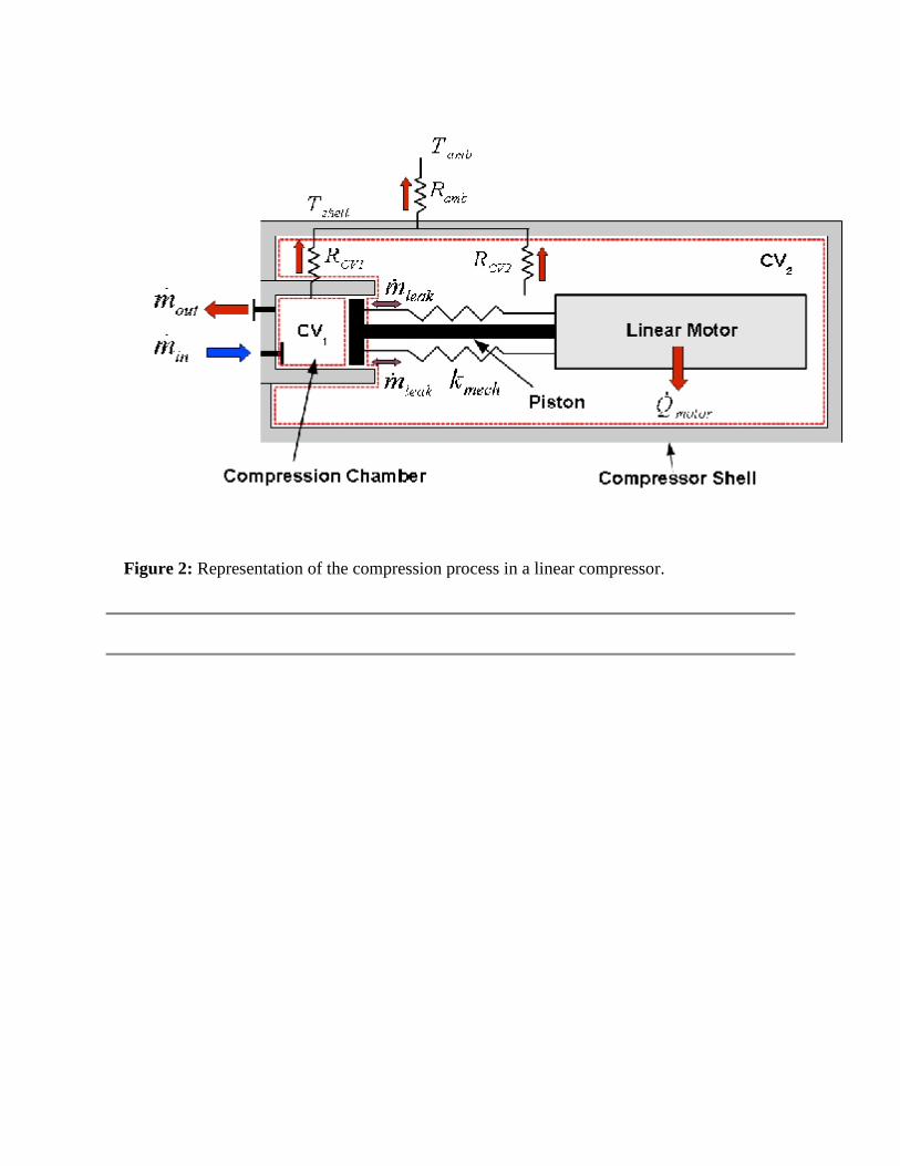
Figure 2: Representation of the compression process in a linear compressor.

Figure 3: Photos of reed valve assembly used in compressor prototype.

Figure 4: Free body diagrams for the valve reed.

Figure 5: Free body diagram of linear compressor piston assembly.

Figure 6: Solution flowchart of linear compressor model (equations solved at each step

given in blocks).

Figure 7: A section view of the prototype linear compressor.

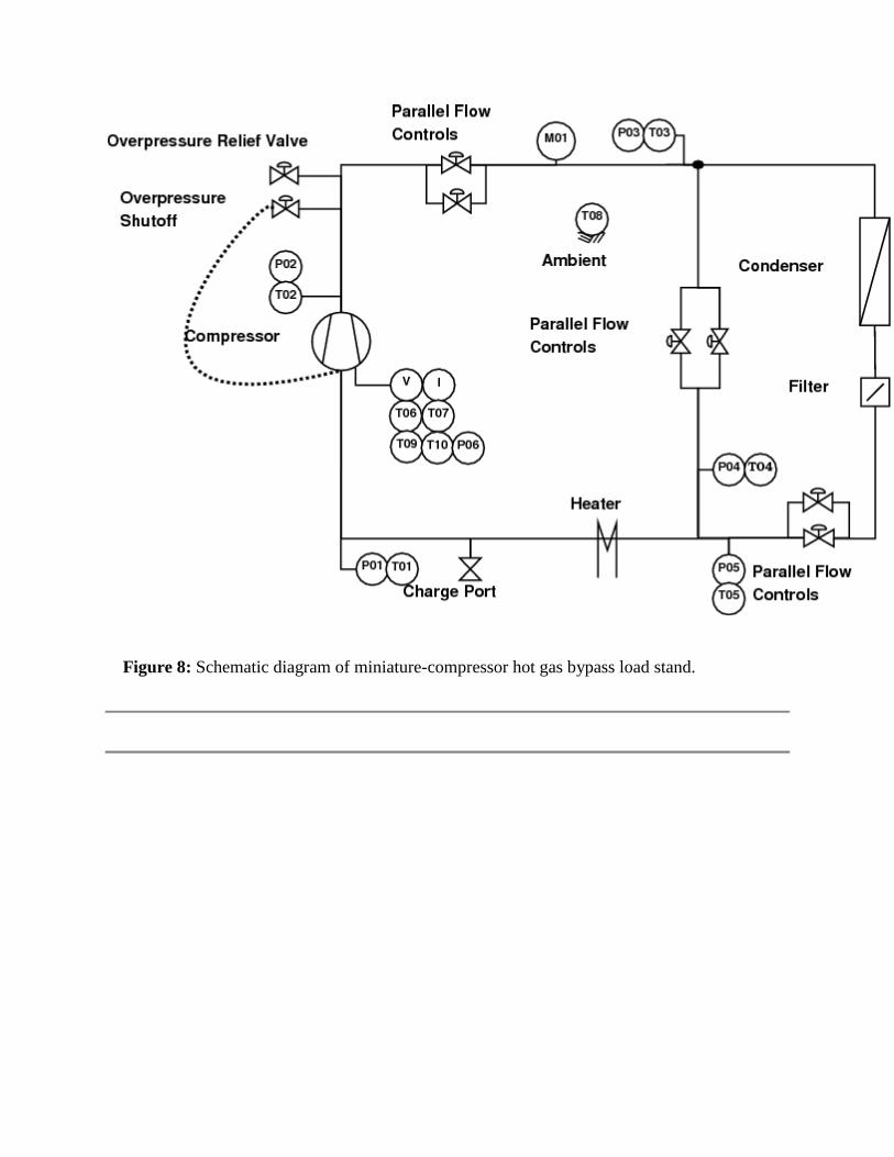
Figure 8: Schematic diagram of miniature-compressor hot gas bypass load stand.

Figure 9: Pressure enthalpy plot of compressor load stand operation.

Figure 10: Comparison of experimental and predicted piston displacements.

Figure 11: Comparison of experimental and predicted mass flow rates.

Figure 12: Comparison of experimental and predicted volumetric efficiencies.

Figure 13: Comparison of experimental and predicted overall isentropic efficiencies.

1 Corresponding Author, cbradsha@purdue.edu