A comparison of multiscale variations of decadelong … ceilometersare ground-basedoptical remote...

A comparison ofmultiscale variations of decade-longcloud fractions from six different platforms overthe Southern Great Plains in the United StatesWei Wu1, Yangang Liu1, Michael P. Jensen1, Tami Toto1, Michael J. Foster2, and Charles N. Long3

1Atmospheric Sciences Division, Brookhaven National Laboratory, Upton, New York, USA, 2Cooperative Institute forMeteorological Satellite Studies, University of Wisconsin, Madison, Wisconsin, USA, 3Pacific Northwest National Laboratory,Richland, Washington, USA

Abstract This study compares 1997–2011 observationally based cloud fraction estimates from six differentplatforms (three ground-based estimates and three satellite-based estimates) over the Southern Great Plains,United States. The comparisons are performed at multiple temporal and spatial scales. The results show that1997–2011mean cloud fractions from the Active Remote Sensing of CLouds (ARSCL) and from the InternationalSatellite Cloud Climatology Project (ISCCP) are significantly (at a 2% significance level, two-sided t test) largerthan the others, having 0.08 and 0.15 larger mean diurnal variations, 0.08 and 0.13 larger mean annualvariations, and 0.08 and 0.14 larger interannual variations, respectively. Although more high (low) cloudsare likely a reason for larger ARSCL (ISCCP) cloud fractions, other mechanisms cannot be ruled out andrequire further investigations. Furthermore, half of the estimates exhibit a significant (at a 1% significancelevel, one-sided t test) overall increase of 0.08–0.10 in the annually averaged cloud fractions from 1998 to 2009;another half of the estimates exhibit little tendency of increase in this decade. Monthly cloud fractions from allthe estimates exhibit quasi-Gaussian frequency distributions while the distributions of daily cloud fractions arefound dependent on spatial scales. Cloud fractions from all the estimates showmuch larger seasonal variationsthan diurnal variations. Findings from this study suggest caution when using observationally based cloudfraction estimates for climate studies such as evaluatingmodel performance and reinforce the need of consistencyin defining and retrieving cloud fractions.

1. Introduction

Cloud fraction (amount) is known to be an important factor in modulating the Earth’s radiation budget[e.g., Wielicki et al., 2002; Loeb et al., 2007; Bender, 2011; Liu et al., 2011]. In climate models, cloud fraction isone of the major parameters in calculation of cloud radiation-precipitation interactions [e.g., Manabe andStrickler, 1964; Ramanathan and Coakley, 1978; Slingo et al., 1989; Sundqvist et al., 1989; Smith, 1990; Tiedtke,1993; Del Genio et al., 1996; Park and Bretherton, 2009; Sokolov and Monier, 2012]. For understanding currentclimate change and predicting future climate variability, observationally based cloud fraction estimateshave been intensively studied for decades [e.g., Minnis, 1989; Wielicki and Parker, 1992; Di Girolamo andDavies, 1997; Rossow and Schiffer, 1999; Clothiaux et al., 2000; Hogan et al., 2001; Kassianov et al., 2005; Longet al., 2006a; Min et al., 2008; Ackerman et al., 2008]. Cloud fraction products retrieved from observationshave been widely used in evaluation of model performance [e.g., Jakob, 1999; Guichard et al., 2003; Bedachtet al., 2007;Wilkinson et al., 2008;Walsh et al., 2009; Ahlgrimm and Köhler, 2010; Bouniol et al., 2010; Kennedyet al., 2011; Wu et al., 2012; Xie et al., 2013].

Before quantitatively comparing different observationally based cloud fraction estimates, it is necessary tounderstand how cloud fraction is defined. Unfortunately, “cloud fraction” or even “a cloud” is not a well-definedquantity. According to the American Meteorological Society Glossary (http://glossary.ametsoc.org/), a cloud isdefined as “a visible aggregate of minute water droplets and/or ice particles in the atmosphere above theEarth’s surface,” and cloud fraction is defined as “the amount of sky estimated to be covered by a specifiedcloud type or level (partial cloud fraction) or by all cloud types and levels (total cloud fraction).” Apparently, thedetermination of whether or not a cloud is present or what fraction of the sky is covered by a cloud isdependent on the observer or on the characteristics of the instrument that is used to make the observations. Inreality, there exist various definitions of cloud fraction, mainly because of the differences in observational

WU ET AL. ©2014. American Geophysical Union. All Rights Reserved. 3438

PUBLICATIONSJournal of Geophysical Research: Atmospheres

RESEARCH ARTICLE10.1002/2013JD019813

Special Section:Fast Physics in Climate Models:Parameterization, Evaluationand Observation

Key Points:• Large differences in the means ofdecade-long cloud fractions

• Different cloud fraction estimatesshow different tendencies of increase

• Cloud fractions at different scales havedifferent distributions

Correspondence to:W. Wu,[email protected]

Citation:Wu, W., Y. Liu, M. P. Jensen, T. Toto,M. J. Foster, and C. N. Long (2014), Acomparison of multiscale variations ofdecade-long cloud fractions from sixdifferent platforms over the SouthernGreat Plains in the United States,J. Geophys. Res. Atmos., 119,3438–3459, doi:10.1002/2013JD019813.

Received 7 MAR 2013Accepted 5 MAR 2014Accepted article online 10 MAR 2014Published online 28 MAR 2014

http://glossary.ametsoc.org/

http://publications.agu.org/journals/

http://onlinelibrary.wiley.com/journal/10.1002/(ISSN)2169-8996

http://dx.doi.org/10.1002/2013JD019813

http://dx.doi.org/10.1002/2013JD019813

http://onlinelibrary.wiley.com/journal/10.1002/(ISSN)2169-8996/specialsection/FASTPHYS1



judywms

Typewritten Text

BNL-104271-2014-JA

instruments, retrieval methods, ormodel parameterizations used todetermine this quantity. Discussionson cloud fraction and its importantrole on determining the Earth’sradiation budget can be found innumerous papers. Among them, athorough and down-to-earthdiscussion on cloud fraction wasgiven by Wiscombe [2005]. Onerelevant key point addressed byWiscombe [2005] is that thedetermination of cloud fractiondepends on wavelength. In otherwords, instruments or a threshold ofradiation properties (dependent onwavelength) used to determine acloud could affect the final productsof cloud fraction. As will bediscussed later in this paper, thedetermination of cloud fraction alsodepends on many other factors

including cloud orientation and morphology, and instrumental viewing geometry and field of view (FOV).Nevertheless, a detailed investigation on causes of the differences in determination of cloud fraction is beyondthe scope of this paper, and the subject of future research.

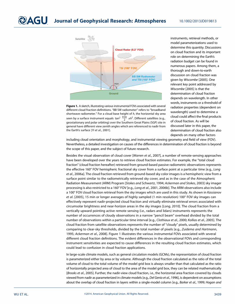
Besides the visual observation of cloud cover [Warren et al., 2007], a number of remote-sensing approacheshave been developed over the years to retrieve cloud fraction estimates. For example, the “total cloudfraction” (cloud fraction hereafter) retrieved from ground-based passive radiometric observations representsthe effective 160° FOV hemispheric fractional sky cover from a surface point at a particular time [e.g., Longet al., 2006a]. The cloud fraction retrieved from ground-based sky color images is a hemispheric view from asurface point similar to the radiometrically retrieved sky cover, and as in the case of the AtmosphericRadiation Measurement (ARM) Program [Stokes and Schwartz, 1994; Ackerman and Stokes, 2003] sky imagerprocessing is also restricted to a 160° FOV [e.g., Long et al., 2001, 2006b]. The ARM observations also includea 100° FOV cloud fraction retrieval from the sky images which are used in this study. As shown in Kassianovet al. [2005], 15 min or longer averages of highly sampled (1 min resolution) 100° FOV sky images caneffectively represent nadir-projected cloud fraction and virtually eliminate retrieval errors associated withcircumsolar brightness and near-horizon areas in the sky images [Long, 2010]. The cloud fraction from avertically upward pointing active remote sensing (i.e., radars and lidars) instruments represents thenumber of occurrences of cloudy observations in a narrow “pencil beam” overhead divided by the totalnumber of observations within a particular time interval [e.g., Clothiaux et al., 2000; Kollias et al., 2005]. Thecloud fraction from satellite observations represents the number of “cloudy” pixels, usually determined bycomparing to clear-sky thresholds, divided by the total number of pixels [e.g., Zuidema and Hartmann,1995; Ackerman et al., 2008]. Figure 1 illustrates the various instrumental FOVs associated with severaldifferent cloud fraction definitions. The evident differences in the observational FOVs and correspondinginstrument sensitivities are expected to cause differences in the resulting cloud fraction estimates, whichcould lead to confusion in cloud fraction applications.

In large-scale climate models, such as general circulation models (GCMs), the representation of cloud fractionis parameterized either by area or by volume. Although the cloud fraction calculated as the ratio of the totalvolume of cloud to the total volume of the model grid box is always smaller than that calculated as the ratioof horizontally projected area of cloud to the area of the model grid box, they can be related mathematically[Brooks et al., 2005]. Further, the nadir-view cloud fraction, i.e., the horizontal area fraction covered by cloudsviewed fromnadir as parameterized in climatemodels [e.g.,Del Genio et al., 1996], is dependent on assumptionsabout the overlap of cloud fraction in layers within a single-model column [e.g., Barker et al., 1999; Hogan and

Figure 1. A sketch, illustrating various instrumental FOVs associatedwith severaldifferent cloud fraction definitions. “BB SW radiometer” refers to “broadbandshortwave radiometer.” For a cloud base height of h, the horizontal sky area

seen by a surface instrument equals tan2 FOV2

� �πh2 . Different satellites (e.g.,

geostationary and polar orbiting) over the Southern Great Plains (SGP) site ingeneral have different view zenith angles which are referenced to nadir fromthe Earth’s surface [Yi et al., 2001].

Journal of Geophysical Research: Atmospheres 10.1002/2013JD019813


Illingworth, 2000;Mace and Benson-Troth, 2002].Although this nadir-view cloud fraction wasalmost unbiased compared to FOV≤ 100°fractional sky cover as mentioned above, it wasfound to always be smaller than ground-based15 min averages of 160° FOV fractional skycover [Kassianov et al., 2005]. The differences ofcloud fraction representations among differentclimate models and between climate modelsand observations pose an additional challengein evaluating modeled cloud fractions.

Although there are numerous studies onevaluation of modeling clouds or cloudimpacts on atmospheric radiation, systematicinvestigations on comparison of multiscalelong-term mean cloud fraction using ground-and satellite-based cloud fraction estimatesare rare. The objective of this paper is tocompare decade-long cloud fraction statisticsat multiple spatial and temporal scales usinghigh-resolution cloud fraction estimates fromsix different platforms over the Southern GreatPlains (SGP) in Oklahoma, United States.Statistical frequency distributions of daily andmonthly cloud fractions are also compared.Statistical significances of the differencesbetween the means and variances of different

cloud fraction estimates are examined. We also provide examples to illustrate potential causes of large cloudfraction differences. Section 2 briefly introduces data and approaches. Section 3 shows results. Sections 4 and5 are discussions and summary.

2. Data and Approaches2.1. Data

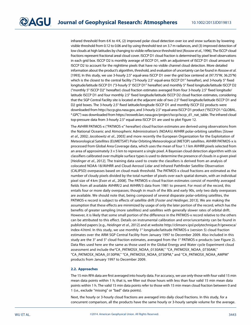
In this study, we compare 1997–2011 observationally based cloud fraction estimates from three ground-based estimates and three satellite-based estimates over the ARM SGP Central Facility (97.485°W, 36.605°N),located in north-central Oklahoma, United States. The three ground-based estimates are from the following:(1) the Active Remote Sensing of CLouds (ARSCL) value-added product, (2) the Total Sky Imager (TSI), and (3)the Radiative Flux Analysis (RFA) based on the Solar and Infrared Radiation System. The three satellite-basedestimates are from the following: (1) the Geostationary Operational Environmental Satellite (GOES), (2) theInternational Satellite Cloud Climatology Project (ISCCP), and (3) the Advanced Very High ResolutionRadiometer (AVHRR) Pathfinder Atmospheres Extended (PATMOS-x). Figure 2 presents the geographiclocation and grid sizes of the cloud fraction estimates investigated in this study.2.1.1. Cloud Fraction Estimates From Ground-Based Active Remote SensingThe ARM SGP Central Facility includes a suite of vertically upward pointing narrow FOV active remote sensorsthat provide detailed observations of the distribution of clouds and hydrometeors within the overlyingatmospheric column. These sensors include a 35 GHz millimeter wavelength cloud radar (MMCR) [Moranet al., 1998], a micropulse lidar (MPL) [Spinhurne, 1993], and a laser ceilometer. None of these sensors candetect all cloud types under all conditions. TheMMCRmaymiss thin clouds, particularly cirrus clouds and thinliquid-water clouds [Turner et al., 2007], and cannot distinguish cloud boundaries from drizzle and heavierprecipitation. The laser instruments cannot penetrate thick low-level clouds and therefore cannot detectcloud layers that lie above them. The MMCR has a 0.2° beam width which results in a horizontal resolution of35 m at a height of 10 km. The MMCR cycles through a sequence of observing modes optimized for theobservation of boundary layer clouds, cirrus clouds, and precipitating clouds [Kollias et al., 2005, 2007a]. The

Figure 2. The geographic locations and grid sizes of the observa-tionally based cloud fraction estimates investigated in this study.The gray solid box represents the SGP Central Facility. The boxesoutlined by colored dashed lines represent spatial scales at thefollowing: (1) 0.5° latitude/longitude (cyan, for GOES), (2) 1° latitude/longitude (red, for GOES and PATMOS-x), (3) 2.5° equal area (orange,for ISCCPD1), (4) 3° latitude/longitude (green, for GOES andPATMOS-x),and (5) 5° latitude/longitude (blue, for GOES, PATMOS-x, ISCCP D1,and ISCCP D2).



MPL and ceilometers are ground-based optical remote sensors that are mainly used for the determination ofthe lowest cloud base, particularly in precipitating conditions where the MMCR has difficulties distinguishingbetween cloud and precipitation particles, and the MPL is also used to supplement the detection of highclouds (when not blocked by lower clouds) that the MMCR cannot detect.

The MMCR observations are combined with the MPL and ceilometer observations to produce best estimatetime-height profiles of hydrometeor locations, radar reflectivites, mean Doppler velocities, and Dopplerspectral widths in the ARSCL value-added product [Clothiaux et al., 2000]. ARSCL provides these profilesbased on sampling on a 10 s, 45 m vertical height interval grid. The cloud frequency of occurrence (cloudfraction hereafter) is estimated as the ratio of the number of 10 s time steps that contain detected clouds tothe total number of time steps within a predetermined time window. This cloud frequency data set isdetermined by the ground-based active remote sensors and used to represent cloud fraction for comparisonsin this study. We use hourly ARSCL total cloud fraction estimates from the ARM Best Estimate (ARMBE) value-added product [Xie et al., 2010] from January 1997 to December 2010. The hourly cloud fraction vertical profiles(based on MMCR and MPL) from the same data file are used to generate Figure 10. The data are available fromNovember 1996 to January 2011 at http://www.arm.gov/sgpcmbe_cldrad_v2.2b_C1.c1. For inhomogeneouscloud cases such as broken clouds or near-cloud field boundaries, the frozen turbulence assumptions inherentin the conversion of cloud frequency of occurrence to cloud fraction may not hold.2.1.2. Cloud Fraction Estimates From Ground-Based Hemispheric ObservationsThere are two separate cloud fraction estimates derived from ground-based hemispheric observations at theARM SGP Central Facility. One is derived from the total sky imager measurements (TSI) and the other frombroadband solar radiometer measurements (RFA).

The TSI captures 24 bit color images of the hemispheric view of the sky at 352×288pixel resolution every 30 s. Acloud decision algorithm uses the ratio of red-to-blue pixel values to determine the presence of clouds overa vertically upward pointing 160° FOV, and also a smaller such as 100° FOV. A user-defined lower limit is set forthe clear-sky red-to-blue ratio value, and any pixels for which the ratio exceeds this clear-sky limit are counted ascloudy. The hemispheric sky cover is then determined as the ratio of the cloudy pixels to the total numberof pixels over the predefined FOV. The cloud decision algorithm is valid for solar elevation angles greater than10° and ignores the 10° of sky near the horizon, giving a FOV of 160°. However, for the large FOV (e.g., 160°),cloud sides may contribute significantly to the total sky cover under partly cloudy skies. Kassianov et al. [2005]analyzed the differences in hemispheric cloud fraction estimates as a function of averaging time, FOV, and cloudspatial structure and found that compared to horizontally projected cloud fraction, a 15 min average of highlysampled sky cover is theminimum time span in order for the “sky cover” to best relate to nadir-projected cloudfraction. They also found that 15min is shown to be the decorrelation time of the sky view, and averaging thatlong with highly sampled data can thus compensate for the individual image view distortion of the cloudelements as they move across the sky view. For the same cloud field, they found that hemispheric-view cloudfraction on average increases as FOV increases. Therefore, we use hourly 100° FOV total sky cover to representthe TSI cloud fraction. The TSI was first deployed at the ARM SGP Central Facility in July 2000; thus, no data isavailable prior to this time. More details about the TSI cloud fraction estimates can be found in Morris [2005].Hourly TSI cloud fraction estimates from July 2000 to August 2011 from the ARMBE products are used in thisstudy. Note that the hourly TSI cloud fraction estimates before 5 April 2005 were retrieved based on a 20° FOVzenith circle. Since the mean diurnal variation from 20° FOV before 5 April 2005 shows an average 0.02difference (i.e., 0.001 to 0.04 difference inmean hourly cloud fractions) compared to that from a 100° FOV zenithcircle after 5 April 2005 (not shown) and the difference of 0.02 is well within the uncertainty of the TSI sky coverretrievals, we include all the hourly TSI cloud fraction estimates from July 2000 to August 2011 for the long-termstatistical comparisons with the assumption that the impact of the TSI zenith FOV switch is minor.

Observations from the direct and diffuse broadband shortwave (SW) radiometers deployed at the ARM SGPCentral Facility are also used to estimate the sky cover. Long and Ackerman [2000] used the observations ofsurface downwelling total and diffuse SW radiation to detect daylight clear-sky time periods for an effective160° FOV from a vertically upward pointing radiometer system. Given a statistically significant subset ofdetected clear-sky observations over the course of a sufficient range of solar zenith angles on given days, dailyclear-sky irradiance functions are fitted, interpolated for cloudy periods, and used to produce continuousestimates of clear-sky total, direct, and diffuse irradiance. This further allows the estimation of the impact ofclouds on the hemispheric radiation field. Long et al. [2006a] used coincident observations from broadband



http://www.arm.gov/sgpcmbe_cldrad_v2.2b_C1.c1

radiometers and carefully screened TSI sky cover to propose a relationship between the impact of clouds onmeasured downwelling diffuse shortwave radiation at the surface and hemispheric sky cover within 160°FOV. In this study, we use the 15 min averages of 160° FOV fractional sky cover (cloud fraction hereafter;data source: “sgp15swfanalsirs1longC1.c1”) from March 1997 to December 2011, available at http://www.arm.gov/instruments/sirs. Based on Long et al. [2006a], the RFA sky cover estimates agree to better than~10% root-mean-square sky cover amount with sky imager retrievals and human observations. In a paperon evaluating representation of cloud properties for three widely used reanalyses (ERA-Interim, NationalCenters for Environmental Prediction (NCEP)/National Center for Atmospheric Research Reanalysis I, andNCEP/Department of Energy Reanalysis II),Wu et al. [2012] used the same 160° FOV RFA cloud fraction estimatesand found that all of the reanalyses exhibit significant underestimation in modeling cloud fraction, surfacerelative shortwave cloud forcing, and cloud albedo. As you will find out later from this paper, the conclusiondrawn by Wu et al. [2012] is well justified at least from the perspective of observed cloud fractions in general.2.1.3. Cloud Fraction Estimates From Satellite-Based Passive Remote SensingThe three satellite-based cloud fraction estimates (GOES, ISCCP, and PATMOS-x) used are brieflyintroduced below.

The GOES NASA (the National Aeronautics and Space Administration)-Langley VISST (Visible Infrared Solar-Infrared Split Window Technique) cloud fraction estimates (“GOES cloud fraction estimates” hereafter) arederived by the NASA Langley cloud and radiation group from multiple GOES passive radiometer observations,including GOES-8 (1997 to March 2003), GOES-10 (April 2003 to July 2006), and GOES-11 (August 2006). It isworth emphasizing that in this paper GOES cloud fraction estimates represent the retrieved cloud fractionproduct from the NASA Langley cloud and radiation group using multiple GOES passive radiometerobservations and thus should not be confused with GOES satellites (e.g., GOES-8 satellite). GOES-10/11 was at135°W whereas GOES-8 was at 75°W. Each GOES pixel (4 km spatial resolution at nadir) is classified as eitherclear or cloudy by comparing the observed visible (0.65 μm) reflectance, solar to infrared (3.8 to 10.8 μm)brightness temperature, and infrared brightness temperature difference to thresholds based on predictedclear-sky values [Minnis et al., 2008]. It is worth mentioning that viewing and solar geometry can impact cloudfraction estimates because of its impact on radiance measurements [e.g., Evan et al., 2007; Kato and Marshak,2009], and the potential impact includes discontinuities of those retrieved cloud fractions from GOES satelliteslocated at different geographic locations. Detailed investigation concerning instrumental calibration and itserror/uncertainty can be found at http://www.oso.noaa.gov/goes/goes-calibration/index.htm. The cloudfraction is estimated as the number of cloudy pixels divided by the total number of pixels in 0.5° latitude/longitude resolution centered at the ARM SGP site (reported as averages approximately every half hour by theMinnis product). Adjacent half-hourly cloud fraction estimates are averaged into the hourly cloud fractionsreported here. In order to investigate impacts of spatial scale on the retrieved cloud fraction, we use the Minnishalf-hourly 0.5° product to generate hourly GOES cloud fraction over 1°, 3°, and 5° domains centered at the ARMSGP Central Facility (see Figure 2). The four sets of hourly GOES cloud fraction estimates from January 1997 toDecember 2011 are used in this study. Data sources are “sgpgoes8minnisX1.c1” for retrievals from 01 January1997 to 30 April 1998, and “sgpvisstgridg*minnisX1.c1” for retrievals from 01 May 1998 to 31 December 2011,where “*” represents “08v2,” “08v3,” “10v2,” “10v3,” “11v3,” “11v4,” or “13v4.” The GOES optical depth product ofcloudy pixels from the same data sources are used to plot Figure 10.

The ISCCP cloud fraction estimates used are total cloud fractions from 3-hourly 2.5° equal-area ISCCP D1, and3-hourly 2.5° fixed latitude/longitude ISCCP D1 andmonthly 2.5° fixed latitude/longitude ISCCP D2 over theARM SGP site from January 1997 to December 2009. The ISCCP cloud fraction estimates were generatedusing the infrared (~ 11 μm) and visible (~ 0.6 μm) radiances from global geostationary (primarily fromthree satellite series: GOES, Geostationary Meteorological Satellite (GMS), and the European MeteorologicalSatellite (Meteosat) and polar-orbiting (AVHRR) meteorological satellites [e.g., Knapp, 2008; Rossow andSchiffer, 1999]. Note that ISCCP D1 and D2 are retrieved primarily based on GOES measurements over theSGP site. However, the ISCCP uses a different cloud detection algorithm and different sampling strategycompared to ARMBE GOES [Minnis et al., 2008]. Descriptions on detection algorithms for ISCCP D-series canbe found in Rossow et al. [1985], Rossow and Garder [1993], and Rossow et al. [1996]. The ISCCP D-series datasets have several improvements compared to their previous version (C-series), including revised radiancecalibrations and reduced biases in cirrus cloud properties. The improvement in cloud detection from ISCCPC-series to ISCCP D-series includes the following: (1) improved cirrus detection over land by lowering



http://www.arm.gov/instruments/sirs

http://www.arm.gov/instruments/sirs

http://www.oso.noaa.gov/goes/goes-calibration/index.htm

infrared threshold from 6K to 4K, (2) improved polar cloud detection over ice and snow surfaces by loweringvisible threshold from 0.12 to 0.06 and by using threshold test on 3.7m radiances, and (3) improved detection oflow clouds at high latitudes by changing to visible reflectance threshold test [Rossow et al., 1996]. The ISCCP cloudfractions represent fractional areal cloud cover. ISCCP D1 cloud fraction is determined by pixel level observationsin each grid box. ISCCP D2 is monthly average of ISCCP D1, with an adjustment of ISCCP D1 cloud amount toISCCP D2 to account for the nighttime pixels that have no visible channel cloud detection. More detailedinformation about the product’s algorithm, threshold, and evaluation of uncertainty can be found in Rossow et al.[1993]. In this study, we use 3-hourly 2.5° equal-area ISCCP D1 over the grid box centered at (97.75°W, 36.25°N)which is the closest to the central facility (“3-hourly 2.5° equal-area ISCCP D1” hereafter), and 3-hourly 5° fixedlongitude/latitude ISCCP D1 (“3-hourly 5° ISCCP D1” hereafter) and monthly 5° fixed longitude/latitude ISCCP D2(“monthly 5° ISCCP D2” hereafter) cloud fraction estimates averaged from four 3-hourly 2.5° fixed longitude/latitude ISCCP D1 and four monthly 2.5° fixed longitude/latitude ISCCP D2 cloud fraction estimates, consideringthat the SGP Central Facility site is located at the adjacent side of two 2.5° fixed longitude/latitude ISCCP D1 andD2 grid boxes. The 3-hourly 2.5° fixed latitude/longitude ISCCP D1 and monthly ISCCP D2 products weredownloaded from http://isccp.giss.nasa.gov, and 3-hourly 2.5° equal-area ISCCP D1 product (“ISCCP.D1.*.GLOBAL.*.GPC”) was downloaded from https://eosweb.larc.nasa.gov/project/isccp/isccp_d1_nat_table. The infrared cloudtop-pressure data from 3-hourly 2.5° equal-area ISCCP D1 are used to plot Figure 12.

The AVHRR PATMOS-x (“PATMOS-x” hereafter) cloud fraction estimates are derived using observations fromthe National Oceanic and Atmospheric Administration’s (NOAA’s) AVHRR polar-orbiting satellites [Stoweet al., 2002; Jacobowitz et al., 2003] and more recently the European Organization for the Exploitation ofMeteorological Satellites (EUMETSAT) Polar Orbiting Meteorological (METOP) satellites. AVHRR PATMOS-x isprocessed from Global Area Coverage data, which uses the mean of four 1.1 km AVHRR pixels selected froman area of approximately 3 × 5 km to represent a single pixel. A Bayesian cloud detection algorithm with sixclassifiers calibrated over multiple surface types is used to determine the presence of clouds in a given pixel[Heidinger et al., 2012]. The training data used to create the classifiers is derived from an analysis ofcolocated NOAA-18/AVHRR and Cloud-Aerosol Lidar and Infrared Pathfinder Satellite Observation(CALIPSO) overpasses based on cloud mask threshold. The PATMOS-x cloud fractions are estimated as thenumber of cloudy pixels divided by the total number of pixels over each spatial domain, with an individualpixel size of 4 km [Evan et al., 2008]. The PATMOS-x cloud fraction estimates consist of monthly averagedfields from all available AVHRR/2 and AVHRR/3 data from 1981 to present. For most of the record, thisentails four or more daily overpasses; though in much of the 80s and early 90s, only two daily overpassesare available. We should note that, being composed of several disparate polar-orbiting satellites, thePATMOS-x record is subject to effects of satellite drift [Foster and Heidinger, 2013]. We are making theassumption that these effects are minimized by usage of only the later portion of the record, which has thebenefits of greater sampling (more satellites) and satellites with generally slower rates of orbital drift.However, it is likely that some small portion of the difference in the PATMOS-x record relative to the otherscan be attributed to this effect. Details on instrumental calibration and error/uncertainty can be found inpublished papers [e.g., Heidinger et al., 2012] and at website http://climserv.ipsl.polytechnique.fr/gewexca/index-4.html. In this study, we use monthly 1° longitude/latitude PATMOS-x (version 5) cloud fractionestimates over the ARM SGP Central Facility from January 1997 to December 2009. Also included in thisstudy are the 3° and 5° cloud fraction estimates, averaged from the 1° PATMOS-x products (see Figure 2).Data files used here are the same as those used in the Global Energy and Water cycle Experiment cloudassessment and include the“CA_PATMOSX_NOAA_0130AM,” “CA_PATMOSX_NOAA_0730AM,”“CA_PATMOSX_NOAA_0130PM,” “CA_PATMOSX_NOAA_0730PM,” and “CA_PATMOSX_NOAA_AMPM”

products from January 1997 to December 2009.

2.2. Approaches

The 15min RFA data are first averaged into hourly data. For accuracy, we use only those with four valid 15minmean data points within 1 h; that is, we filter out those hours with less than four valid 15 min mean datapoints within 1 h. The valid 15 min data points refer to those with 15 min mean cloud fraction between 0 and1 (i.e., exclude “missing” or “bad” data points).

Next, the hourly or 3-hourly cloud fractions are averaged into daily cloud fractions. In this study, for aconcurrent comparison, all the products have the same hourly or 3-hourly sample volume for the average.



http://isccp.giss.nasa.gov

https://eosweb.larc.nasa.gov/project/isccp/isccp_d1_nat_table

http://climserv.ipsl.polytechnique.fr/gewexca/index-4.html

http://climserv.ipsl.polytechnique.fr/gewexca/index-4.html

However, for a comparison without concurrency, each product has its own hourly or 3-hourly sample volumefor the average which includes all available valid data points. The daily cloud fractions are averaged intomonthly cloud fractions and then further averaged into yearly cloud fractions. The mean diurnal, annual, andinterannual variations of cloud fraction from all the estimates are then compared. Note that, “concurrent validdata point” in the comparisons refers to a data point commonly valid for all the compared estimates. To makecomparisons on mean diurnal variations, a concurrent 3-hourly cloud fraction refers to a valid 3-hourly cloudfraction under the condition that within the 3-hour window, all the hourly cloud fraction estimates used incomparison have valid data points. For those cloud fraction estimates with a “flag” indicating the number ofvalid data points originally used in generating the estimates, including the hourly ARSCL, TSI, GOES, and3-hourly 2.5° fixed latitude/longitude ISCCP D1, we use only those generated from more than 50% valid datapoints. Likewise, only those cloud vertical profiles which satisfy the condition of more than 50% lidar/ceilometer valid data points within each hour in determination of cloud base are used to generate Figure 10.Hourly or 3-hourly standard deviations are calculated for each specific hour or 3 h of a day using hourly or3-hourly data for all the days over all the years. Monthly standard deviations are calculated for each specificmonth of a year using monthly data over all the years. Yearly standard deviations are calculated usingmonthly data for each specific year after removing mean seasonal variation, that is, the averages of monthlycloud fraction for each specific month of a year over all years.

3. Results

In this section, we compare mean diurnal, annual, and interannual variations of all-sky cloud fraction from allthe estimates (without or with concurrency). Note that in this paper, unless otherwise specified, “daytime”

0.3

0.4

0.5

0.6

0.7 a

0.3

0.4

0.5

0.6

0.7 b

0.3

0.4

0.5

0.6

0.7

All−

Sky

Clo

ud

Fra

ctio

n

c

0 6 12 18 240.3

0.4

0.5

0.6

0.7 d

Local Hour

e

f

g

2 4 6 8 10 12

h

Month

i

j

k

98 00 02 04 06 08 10

l

Year

Figure 3. The 1997–2011mean (a–d) diurnal, (e–h) annual, and (i–l) interannual variations of all-sky cloud fractions from sixdifferent ground- and satellite-based cloud fraction estimates over the ARM SGP site, Oklahoma, United States. Colors andlines: (1) the cyan lines represent ARSCL cloud fractions; (2) the green lines represent TSI cloud fractions; (3) the blue linesrepresent 160° FOV RFA cloud fractions; (4) the red solid, dashed, dotted, and dash-dotted lines represent GOES cloud fractionsover 0.5°, 1°, 3°, and 5° latitude/longitude grid boxes, respectively; (5) the black solid, dashed, and dotted lines represent PATMOS-xcloud fractions over 1°, 3°, and 5° latitude/longitude grid boxes, respectively; (6) the brown solid, dashed, and dotted linesrepresent 2.5° equal-area ISCCP D1, 5° latitude/longitude ISCCP D1, and 5° latitude/longitude ISCCP D2 cloud fractions. Blacktriangles, circles, and squares represent mean diurnal variations from 1°, 3°, and 5° PATMOS-x cloud fractions.



refers to “6A.M. to 6 P.M. localstandard time (LST)” (nominaldaytime), “nighttime” refers to“6 P.M. to next-day 6 A.M. LST”(nominal nighttime), “all-sky”refers to “cloud fraction ≥ 0,” and“cloudy sky” refers to “cloudfraction ≥ 0.01.”

3.1. Comparisons WithoutConcurrency3.1.1. Mean Diurnal, Annual,and Interannual Variations ofAll-Sky Cloud FractionsFigure 3 shows mean diurnal,annual, and interannual variations

of all-sky cloud fractions from all the estimates. It is notable that the mean cloud fractions from ISCCP andARSCL aremuch larger than those from the rest of the cloud fraction estimates (TSI, RFA, GOES, and PATMOS-x),that is, 0.15 (ISCCP) and 0.08 (ARSCL) larger in the averaged mean diurnal variations, 0.13 (ISCCP) and 0.08(ARSCL) larger in the averagedmean annual variations, and 0.14 (ISCCP) and 0.08 (ARSCL) larger in the averagedinterannual variations. In particular, the ISCCP or ARSCL mean monthly cloud fractions in January equals 0.69–0.70 or 0.56, which are 0.21–0.22 or 0.08 larger than the average (0.48) from the rest of the estimates that aresimilar in their overall magnitudes.

The 1997–2011 mean annual variations from ARSCL, TSI, and RFA look similar to one another and to thosefrom 1997 to 2008 ARSCL, TSI, and RFA reported by Qian et al. [2012]. The 1997–2011 mean annual totalcloud fraction of 53.89% from the ARMBE ARSCL is the same as the 1998–2004 ARM ARSCL mean totalcloud fraction of 54% obtained by Kollias et al. [2007b, Table 1], similar to the 1997–2008 ARM ARSCL meantotal cloud fraction of 51% obtained by Qian et al. [2012, Table 2] and the 1997–2010 ARM ARSCL meantotal cloud fraction of 55% obtained by Kennedy et al. [2013, Table 5]. However, the much larger meancloud fractions from the ARMBE ARSCL (retrieved based on radar, lidar, and laser ceilometer observations)than those from 0.5° GOES seem inconsistent with the result by Xi et al. [2010], where they compared1997–2006 mean total cloud fraction (46.9%) derived from radar-lidar-based cloud fractions (the sameinstrument data streams as the ARSCL) and from 0.5° GOES over the SGP site and concluded that they havean excellent agreement. Kennedy et al. [2013, section 5] found the same discrepancy compared to Xi et al.[2010] and attributed it to the fact that Xi et al. [2010] used the MPL measurements only as a constraint onMMCR cloud bases. We also used current ARMBE ARSCL data and found that the 1997–2006 ARSCL meantotal cloud fraction from MMCR-only measurements (i.e., the data quality flag “qc_cld_frac_source”indicates “mostly from MMCR,” referring to the case that MPL was not working or did not have valid data,and MMCR had valid values, based on the ARMBE ARSCL data center) equals 47.03%, similar to the 1997–2006radar-lidar-based mean total cloud fraction (46.9%) by Xi et al. [2010]. Furthermore, the mean total cloudfractions from the same product but at different temporal and spatial scales (2.5° equal-area ISCCP D1, 5°ISCCP D1 and ISCCP D2; 0.5°/1°/3°/5° GOES; 1°/3°/5° PATMOS-x) in Figure 3 show generally similar meandiurnal, annual, and interannual variations with minor (<0.05) differences. This is partially consistent withthe result in Xi et al. [2010] that GOES’s decade-long mean cloud fraction over the SGP site is insensitive tothe spatial resolution from 0.5° to 2.5°.

It is worth noting that 1997–2011 ARSCL mean annual total cloud fraction from MMCR-only measurements(calculated from> 50% valid points) equals 0.45, which is not far from the average of the mean annual totalcloud fraction (0.54� 0.08 = 0.46) from the TSI, RFA, GOES, and PATMOS-x cloud fraction estimates. In otherwords, the relatively large cloud fraction in ARSCL is probably associated with lidar (MPL) measurements.Also, one might expect greater consistency between PATMOS-x and ARSCL, as the PATMOS-x Bayesian clouddetection algorithm uses the CALIPSO lidar as training data. A likely cause of the difference in between is thatPATMOS-x is constrained by the sensitivity of the AVHRR sensors, which may not provide sufficientradiometric contrast to detect subvisible cirrus regardless of the training data used.

Table 1. Sample Statistics of 1997–2011 Monthly Cloud Fractions Over theARM SGP Site

Total Valid Months Mean Standard Deviation

ARSCL 169 0.54 0.12TSI 133 0.44 0.12RFA 178 0.47 0.120.5° GOES 180 0.46 0.111° GOES 180 0.46 0.113° GOES 180 0.46 0.115° GOES 180 0.47 0.102.5° Equal-Area ISCCP D1 156 0.58 0.125° ISCCP D1 156 0.60 0.115° ISCCP D2 156 0.61 0.111° PATMOS-x 156 0.45 0.113° PATMOS-x 156 0.46 0.105° PATMOS-x 156 0.46 0.09



For the mean diurnal variations, all the estimates show the smallest cloud fraction of 0.40 to 0.59 at 6 P.M. Themajority of the estimates show an increase of 0.02 to 0.03 from early morning to noon and a decrease of 0.02to 0.06 from noon to late afternoon.

For the mean annual variations, all the estimates exhibit large mean cloud fractions in winter and springseasons, with a peak in January for 5° ISCCP D1, in February for ARSCL, GOES, and 3°/5° PATMOS-x, or in Marchfor 2.5° equal-area ISCCP D1 and 5° ISCCP D2, 1° PATMOS-x, TSI, and RFA. The smallest mean cloud fraction isshown in summer and early fall, that is, in July for ISCCP D2 and RFA; in July and September for 2.5° equal-areaand 5° ISCCP D1, in August and September for TSI; or in September for ARSCL, GOES, and PATMOS-x.

The interannual variations exhibit different tendencies: three of the estimates (from ISCCP, ARSCL, and GOES)show an overall increase of 0.08–0.10 in the annually averaged cloud fraction from 1998 to 2009; however,the other three estimates (from TSI, RFA, and PATMOS-x) exhibit little tendency of increase in the annuallyaveraged cloud fractions in the same decade. It is worth further investigation to determine how the cloudfraction tendency links to the findings in a published paper of global brightening over the SGP [Long et al.,2009]. The standard deviations of the mean cloud fractions are shown in Figure 4. As can be seen, thestandard deviations of the mean hourly or 3-hourly cloud fractions range from 0.07 to 0.18. GOES showsrelatively larger standard deviation near midnight, TSI and RFA show relatively larger standard deviations inthe morning and afternoon, respectively, and the rest of the estimates are evenly distributed throughout theday. Note that, the GOES midnight IR calibration issue [e.g., Yu et al., 2013] could be associated with therelatively larger GOES cloud fraction’s standard deviation at midnight, whereas the ISCCP does not have themidnight issue (although retrieved mostly using GOES measurements over the SGP site) is probably because

Table 2. Results of Statistical Significance Based on Student t test and f testa

Student t Test for the Differences Between the Means of Different Monthly Cloud Fraction EstimatesARSCL TSI RFA 0.5° G 1° G 3° G 5° G 2.5° I (D1) 5° I (D1) 5° I (D2) 1° P 3° P 5° P

ARSCL N/A S S S S S S S S S S S STSI 6.91 N/A NS NS NS NS S S S S NS NS NSRFA 5.06 2.31 N/A NS NS NS NS S S S NS NS NS0.5° G 6.24 1.44 1.04 N/A NS NS NS S S S NS NS NS1° G 6.67 1.02 1.49 0.47 N/A NS NS S S S NS NS NS3° G 6.42 1.40 1.13 0.08 0.40 N/A NS S S S NS NS NS5° G 5.46 2.54 0.01 1.14 1.63 1.24 N/A S S S NS NS NS2.5° I (D1) 3.23 10.08 8.43 9.74 10.18 10.00 9.15 N/A NS NS S S S5° I (D1) 4.48 11.68 9.95 11.40 11.85 11.71 10.89 1.12 N/A NS S S S5° I (D2) 5.70 12.84 11.20 12.69 13.14 13.03 12.25 2.35 1.30 N/A S S S1° P 6.74 0.81 1.67 0.68 0.22 0.62 1.84 10.21 11.94 13.21 N/A NS NS3° P 6.56 1.08 1.41 0.40 0.07 0.33 1.57 10.09 11.85 13.14 0.29 N/A NS5° P 6.05 1.81 0.73 0.35 0.83 0.43 0.82 9.71 11.53 12.87 1.05 0.77 N/A

f Test for the Differences Between the Variances of Different Monthly Cloud Fraction EstimatesARSCL TSI RFA 0.5° G 1° G 3° G 5° G 2.5° I (D1) 5° I (D1) 5° I (D2) 1° P 3° P 5° P

ARSCL N/A NS NS NS NS NS S NS NS NS NS NS STSI 1.12 N/A NS NS NS NS NS NS NS NS NS NS SRFA 1.10 1.01 N/A NS NS NS NS NS NS NS NS NS S0.5° G 1.26 1.13 1.14 N/A NS NS NS NS NS NS NS NS NS1° G 1.26 1.13 1.14 1.00 N/A NS NS NS NS NS NS NS NS3° G 1.36 1.22 1.24 1.08 1.08 N/A NS NS NS NS NS NS NS5° G 1.54 1.37 1.39 1.22 1.22 1.13 N/A NS NS NS NS NS NS2.5° I (D1) 1.08 1.03 1.02 1.17 1.17 1.26 1.17 N/A NS NS NS NS S5° I (D1) 1.31 1.17 1.19 1.04 1.04 1.04 1.42 1.21 N/A NS NS NS NS5° I (D2) 1.29 1.15 1.17 1.02 1.02 1.06 1.19 1.19 1.02 N/A NS NS NS1° P 1.38 1.23 1.25 1.10 1.10 1.01 1.11 1.28 1.06 1.07 N/A NS NS3° P 1.48 1.32 1.34 1.17 1.17 1.08 1.04 1.37 1.13 1.15 1.07 N/A NS5° P 1.73 1.55 1.57 1.37 1.37 1.27 1.13 1.60 1.32 1.34 1.25 1.17 N/A

aThe two-sided critical t value for degree of freedom great than 120 (which applies to all the cases here) at a 2% significance level is set to be the t value (2.36) fordegree of freedom of 120. The one-sided critical f value for degree of freedombetween 100 and 200 for both numerator and denominator (which applies to all thecases here) at a 1% significance level is set to be the mean value (1.50) of the f values when degree of freedoms of numerator and denominator being 100 and 100(f value: 1.60), 100 and 200 (f value: 1.48), 200 and 100 (f value: 1.52), and 200 and 200 (f value: 1.39). Here one-sided f values are calculated using larger variancedivided by smaller variance [Caulcutt, 1991]. “G,” “I,” and “P” represent “GOES,” “ISCCP,” and “PATMOS-x,” respectively. “2.5° I (D1)” refers to “2.5° Equal-Area ISCCPD1.” “S” or “NS” refer to “significant” or “not significant,” respectively. “N/A” refers to “not apply.” All the numbers representing “significant” are marked in bold.



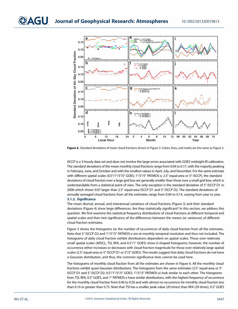
ISCCP is a 3-hourly data set and does not involve the large errors associated with GOES midnight IR calibration.The standard deviations of themeanmonthly cloud fractions range from0.04 to 0.17, with themajority peakingin February, June, and October and with the smallest values in April, July, and December. For the same estimatewith different spatial scales (0.5°/1°/3°/5° GOES; 1°/3°/5° PATMOS-x; 2.5° equal-area or 5° ISCCP), the standarddeviations of cloud fraction over a large grid box are generally smaller than those over a small grid box, which isunderstandable from a statistical point of view. The only exception is the standard deviation of 5° ISCCP D1 in2006 which shows 0.07 larger than 2.5° equal-area ISCCP D1 and 5° ISCCP D2. The standard deviations ofannually averaged cloud fractions from all the estimates range from 0.04 to 0.14, varying from year to year.3.1.2. SignificanceThe mean diurnal, annual, and interannual variations of cloud fractions (Figure 3) and their standarddeviations (Figure 4) show large differences. Are they statistically significant? In this section, we address thisquestion. We first examine the statistical frequency distributions of cloud fractions at different temporal andspatial scales and then test significance of the differences between the means (or variances) of differentcloud fraction estimates.

Figure 5 shows the histograms (or the number of occurrence) of daily cloud fraction from all the estimates.Note that 5° ISCCP D2 and 1°/3°/5° PATMOS-x are at monthly temporal resolution and thus not included. Thehistograms of daily cloud fraction exhibit distributions dependent on spatial scales. Those over relativelysmall spatial scales (ARSCL, TSI, RFA, and 0.5°/1° GOES) show U-shaped histograms; however, the number ofoccurrence either increases or decreases with cloud fraction magnitude for those over relatively large spatialscales (2.5° equal-area or 5° ISCCP D1 or 3°/5° GOES). The results suggest that daily cloud fractions do not havea Gaussian distribution, and thus, the common significance tests cannot be used here.

The histograms of monthly cloud fraction from all the estimates are shown in Figure 6. All the monthly cloudfractions exhibit quasi-Gaussian distributions. The histograms from the same estimates (2.5° equal-area or 5°ISCCP D1 and 5° ISCCP D2; 0.5°/1°/3°/5° GOES; 1°/3°/5° PATMOS-x) look similar to each other. The histogramsfrom TSI, RFA, 0.5° GOES, and 1° PATMOS-x have similar distributions, with the highest frequency of occurrencefor the monthly cloud fraction from 0.40 to 0.50 and with almost no occurrence for monthly cloud fraction lessthan 0.10 or greater than 0.75. Note that TSI has a smaller peak value (20 times) than RFA (29 times), 0.5° GOES

0.05

0.10

0.15a

0.05

0.10

0.15b

0.05

0.10

0.15

Sta

nd

ard

Dev

iati

on

of

All−

Sky

Clo

ud

Fra

ctio

n

c

0 6 12 18 24

0.05

0.10

0.15

Local Hour

d

e

f

g

2 4 6 8 10 12

h

Month

i

j

k

98 00 02 04 06 08 10

l

Year

Figure 4. Standard deviations of mean cloud fractions shown in Figure 3. Colors, lines, and marks are the same as Figure 3.



(30 times) or 1° PATMOS-x (31 times), probably because TSI has fewer valid monthly cloud fractions than RFA,0.5° GOES or 1° PATMOS-x. However, the histograms from 2.5° equal-area ISCCP D1 and ARSCL show differentdistributions when compared to those from the other estimates. For the monthly cloud fraction, 2.5° equal-areaISCCP D1 and ARSCL have the highest frequency of occurrence from 0.62 to 0.68 and from 0.55 to 0.60,respectively, much larger than the other estimates. The largest monthly cloud fractions from (2.5° equal-area or5°) ISCCP and ARSCL are the same (0.82), much larger than those (0.72–0.75) from the other estimates. Likewise,the smallest monthly cloud fractions from (2.5° equal-area or 5°) ISCCP and ARSCL are 0.27–0.35 and 0.25, muchlarger than those (0.15–0.21) from the other estimates. Note that the U-shaped frequency distributions of dailycloud fraction and the quasi-Gaussian distributions of monthly cloud fraction from ARSCL, TSI, and RFA ingeneral look similar to those reported by Qian et al. [2012], obtained from 1997 to 2008 concurrent daily and

0 0.2 0.4 0.6 0.80

500

1000 ARSCL

TSI

RFA

0.5o GOES

2.5o Equal−Area ISCCP D1

a

Nu

mb

er o

f O

ccu

rren

ce

0 0.2 0.4 0.6 0.8

0.5o GOES

1o GOES

3o GOES

5o GOES

b

Daily Cloud Fraction0 0.2 0.4 0.6 0.8 111

2.5o Equal−Area ISCCP D1

5o ISCCP D1

c

Figure 5. The histograms of 1997–2011 daily cloud fractions from all the estimates. Colors and lines are the same as inFigures 3 and 4.

0

10

20

30

40 ARSCLTSIRFA0.5o GOES1o PATMOS−x2.5o Equal−

Area ISCCP D1

a0.5o GOES1o GOES3o GOES5o GOES

b

0 0.2 0.4 0.6 0.8 10

10

20

30

40 2.5o Equal−Area ISCCP D15o ISCCP D15o ISCCP D2

c

Monthly Cloud Fraction

Nu

mb

er o

f O

ccu

rren

ce

0 0.2 0.4 0.6 0.8 1

1o PATMOS−x3o PATMOS−x5o PATMOS−x

d

Figure 6. The histograms of 1997–2011 monthly cloud fractions from all the estimates. Colors and lines are the same as inFigures 3–5.



monthly cloud fractions. The only exception is that ARSCL daily cloud fractions with magnitude <0.10 in Qianet al. [2012] do not have high occurrence as shown in Figure 5.

The autospectral density distributions and autocovariance distributions of monthly cloud fraction from all theestimates are further examined (not shown). Results show that the monthly cloud fractions from TSI and RFAdo not have a periodic signal (a peak at a certain frequency); the monthly cloud fractions from the otherestimates include either a weak (ARSCL, GOES, and PATMOS-x) or a relatively strong (ISCCP) narrow-bandsignal with a frequency of 1 year�1.

The quasi-Gaussian distributions of all the monthly cloud fractions permit an examination of significance ofthe differences between the means or variances from different cloud fraction estimates using Student’s t testor f test. Table 1 lists sample statistics of monthly cloud fraction estimates, including validmonths, means, andstandard deviations which were calculated without removing mean seasonal variation. Table 2 lists theresults from the statistical significance tests for monthly cloud fractions. The formulas and requirements ofthe significance tests can be found in a general statistical book [e.g., Bendat and Piersol, 1986; Caulcutt, 1991]and thus omitted here.

Table 2 (2) shows that at a 1% significance level (one-sided f test) the difference of the variances fromdifferent monthly cloud fraction estimates are not significant except for ARSCL versus 5° GOES, and 5°PATMOS-x versus ARSCL/TSI/RFA/2.5° equal-area ISCCP D1. Table 2 (1) shows that at a 2% significance level(two-sided t test) both ARSCL and ISCCP mean cloud fractions exhibit statistically significant differencescompared to themean cloud fractions from all the other estimates, except for 2.5° equal-area ISCCP D1 versus5° ISCCP D1, 2.5° equal-area ISCCP D1 versus 5° ISCCP D2, and 5° ISCCP D1 versus 5° ISCCP D2. TSI mean cloudfraction also shows a statistically significant difference compared to 5° GOES mean cloud fraction. Except forthe cases mentioned above, the mean cloud fractions from all the other estimates do not show a statisticalsignificance. It is worth mentioning that if using a more permissive 5% significance level: (1) the two-sidedcritical t value will be 1.98, and thus, it does not change the results except that the two pairs (TSI versusRFA and 2.5° Equal-Area ISCCP D1 versus 5° ISCCP D2) are now determined to be significantly different; (2)the one-sided critical f value will be 1.33, and thus, it does not change the results except that those pairs(3° GOES versus ARSCL, 5° GOES versus TSI/RFA, 1° PATMOS-x versus ARSCL, 3° PATMOS-x versus ARSCL/RFA, 5° PATMOS-x versus 0.5°/1° GOES, and 5° PATMOS-x versus 5° ISCCP D2) are now determined to besignificantly different. Overall, 5% significance level seems a too permissive threshold for this analysis.

The statistical significance of the overall increase of 0.08–0.10 in the annually averaged cloud fractions from1998 to 2009 in three of the estimates (ISCCP, ARSCL, and GOES) is also examined using a standard procedure/method that can be found in a general statistics book [e.g., Caulcutt, 1991, chapter 10]. Basically, a linearregression fit was first conducted, and then Student’s t test was applied to determine the significance of theestimated trend. For the annually averaged cloud fractions, the calculated Student’s t values are 5.47, 6.05,5.25, 2.48, and 4.87/4.09/4.81/5.76 for 2.5° equal-area ISCCP D1, 5° ISCCP D1, 5° ISCCP D2, ARSCL, and 0.5°/1°/3°/5° GOES, which are all greater than the critical t value 2.36 at a 1% significance level (one-sided t test) witha degree of freedom of 120. Note that the degrees of freedom for all the cases here are greater than 120,corresponding to smaller critical t values than those with a degree of freedom of 120. In other words, theoverall increase of 0.08–0.10 from 1998 to 2009 in ISCCP, ARSCL, and GOES are significant at a 1% significancelevel. Of course, a more permissive 5% significance level leads to a smaller critical t value of 1.66 (one-sidedand with a degree of freedom of 120) and thus does not change the results of significance test. Nevertheless,it is worth mentioning that decade-long annually averaged cloud fractions may not be statistically longenough to state “trend.”

3.2. Comparisons With Concurrency

Based on the results shown in section 3.1, (2.5° equal-area or 5°) ISCCP and ARSCL cloud fractions aresignificantly larger than other estimates. Could the disagreement be caused by the different volumes ofhourly or 3-hourly data points used in the comparisons? In this section, we examine this issue by usingconcurrent hourly and 3-hourly cloud fractions. The cloudy times from hourly or 3-hourly cloud fractions referto the total number of hourly cloudy times or the total number of 3-hourly cloudy times.

Figure 7 shows mean diurnal, annual, and interannual variations of all-sky cloud fractions from concurrentdaytime (2001–2010) or nighttime (1997–2010) all-sky hourly or 3-hourly cloud fractions. The daytime or



nighttime mean cloud fractions from 2.5° equal-area ISCCP D1, 5° ISCCP D1, and ARSCL are 0.02 to 0.30 largerthan those from the rest of the estimates all day and throughout the year, except for daytime 2.5° equal-areaISCCP D1 from December to March when the mean cloud fractions from 2.5° equal-area ISCCP D1 and TSI/RFA/GOES are comparable, and except for nighttime 5° ISCCP D1 and ARSCL from June to August when themean cloud fractions from 5° ISCCP D1 and ARSCL are comparable to those from 0.5°/1°/3°/5° GOES. Inparticular, 5° ISCCP D1 or ARSCL daytimemeanmonthly cloud fraction in January equals 0.71 or 0.55, which is0.26 or 0.10 larger than the average (0.45) from TSI, RFA, and 0.5°/1°/3°/5° GOES. In January, 5° ISCCP or ARSCLnighttime mean monthly cloud fraction equals 0.67 or 0.55, which is 0.24 or 0.11 larger than the average(0.43) of all the other estimates (0.5°/1°/3°/5° GOES). Both daytime and nighttime 2.5° equal-area ISCCP D1cloud fractions are smaller than the corresponding 5° ISCCP D1 from December to March. Daytime meandiurnal cloud fractions from 2.5° equal-area ISCCP D1 is 0.05 to 0.09 smaller than those from 5° ISCCP D1 from9A.M. to 6 P.M. Daytime mean monthly cloud fractions from 2.5° equal-area ISCCP D1 are comparable to 5°ISCCP D1 from April to October except that in September, the former is 0.13 larger than the latter, and inNovember, the former is 0.09 smaller than the latter. Nighttime 2.5° equal-area ISCCP D1 cloud fractions fromApril to October are 0.02 to 0.14 larger than 5° ISCCP D1 cloud fractions, and in November, their cloud fractionsare comparable. Nighttime 2.5° equal-area ISCCP D1 and 5° ISCCP D1 have a comparable magnitude in theirmean 3-hourly cloud fractions. As expected, the annually averaged cloud fractions from 2.5° equal-area ISCCP D1,5° ISCCP D1, and ARSCL are much larger than those from the rest of the estimates, except for daytime 2.5° equal-area ISCCP D1 from 2003 to 2005, nighttime 2.5° equal-area ISCCP D1 in 2004 and 2005, and nighttime ARSCL in2007 that show similar cloud fractions to those from the rest of the estimates. It is worthmentioning that there isa large difference between the concurrentmean cloud fractions from 3-hourly 2.5° equal-area ISCCP D1 and from3-hourly 5° ISCCP D1. Different geographical sizes might be one cause, considering of geographical significanceof cloud inhomogeneity which we do not see from 0.5°/1°/3°/5° GOES data sets.

The mean diurnal, annual, and interannual variations of daytime all-sky cloud fraction from 0.5°/1°/3°/5°GOES, TSI, and RFA are close to each other, with differences no more than 0.08; however, the total numbers of

0.4

0.5

0.6

0.7

0.8

Clo

ud

Fra

ctio

n (

D)

a

1000

2000

3000

4000

5000

Clo

ud

y T

imes

(D

) b

e

f

i

j

0.4

0.5

0.6

0.7

0.8

Clo

ud

Fra

ctio

n (

N)

c

0 6 12 18 24

1000

2000

3000

4000

5000

Local Hour

Clo

ud

y T

imes

(N

) d

g

2 4 6 8 10 12Month

h

k

98 00 02 04 06 08Year

l

Figure 7. The 2001–2010mean (a and b) diurnal, (e and f) annual, and (i and j) interannual variations of concurrent daytimeall-sky hourly or 3-hourly cloud fractions, and 1997–2010 mean (c and d) diurnal, (g and h) annual, and (k and l) interannualvariations of concurrent nighttime all-sky hourly or 3-hourly cloud fractions. Colors and lines are the same as in Figures 3–6,except that the purple lines in Figures 7b, 7d, 7f, 7h, 7j, and 7l represent 3-hourly 5° GOES cloud fractions. Note that, except for3-hourly 5° GOES, 3-hourly 2.5° equal-area ISCCP D1, and 3-hourly 5° ISCCP D1, all the others are from hourly cloud fractions.



their cloudy times can differ largely. For example, for the daytime case, 0.5° GOES has no more than 0.07difference in the 2001–2010 mean monthly cloud fractions from TSI and RFA, but its hourly cloudy times in amonth (for example, 1885 times in July) can differ largely compared to those from TSI (2319 times in July) andRFA (2442 times in July). In other words, the relatively small differences in the 2001–2010 daytime meanmonthly cloud fractions do not indicate a good agreement on daytime hourly cloud fraction time series.Likewise, the mean annual variations of nighttime all-sky cloud fraction from 0.5°/1°/3°/5° GOES are close toeach other, with difference no more than 0.04. For both daytime and nighttime cases, the mean diurnal,annual, and interannual variations of 0.5°/1°/3°/5° GOES cloud fractions are close to each other (withdifference no more than 0.02 for the daytime case and no more than 0.04 for the nighttime case), similar toFigure 3. The GOES cloudy times averaged over a large spatial scale are larger than those over a small spatialscale, which is not a surprise because a cloud must exist over a large spatial area if a cloud exists over a smallspatial area inside the large area but the opposite is not true. As can be seen from Figure 7, the difference innighttime cloudy times are larger than that in daytime cloudy times, and 3-hourly 2.5° equal-area ISCCP D1, 5°ISCCP D1, and 5° GOES have a good agreement in their daytime and nighttime cloudy times. Overall, themajority of the estimates show the largest frequency of daytime clouds in May and relatively low frequency ofdaytime clouds from November to February, and the least nighttime cloudy times in September andrelatively large nighttime cloudy times from May to July.

The corresponding standard deviations of the concurrent mean cloud fractions are shown in Figure 8. Themajority of the standard deviations range from 0.04 to 0.17, peaking in June, October, and December that areprobably linked to relatively large standard deviations in late afternoon and near midnight. In general, the2.5° equal-area ISCCP D1 has larger standard deviations when compared against that of the other estimates,the exceptions being in August and September.

4. Discussions

Section 3 shows that there exists a substantial disagreement between different cloud fraction estimates. Inparticular, ARSCL and ISCCPmonthly mean cloud fractions show statistically significant differences comparedto those from the rest of the estimates based on a two-sided t test at a 2% significance level. This sectionbriefly discusses some potential issues relevant to the large differences.

The contour pairs in Figure 9 show the joint frequency distributions of concurrent daytime hourly cloudfractions. The majority of the hourly cloud fractions from all the estimates are basically divided into twopopulations: cloud fractions greater than 0.80 or less than 0.20, consistent with the U-shaped frequencydistribution previously reported by Hogan et al. [2001], although there are notable differences in the details.The majority of hourly ARSCL cloud fractions are either greater than 0.90 or less than 0.20. For a large portionof the ARSCL cloud fractions that are >0.90, the corresponding TSI, RFA, or 0.5° GOES cloud fractions exhibit

0.1

0.2

0.3 b c

0 6 12 18 24

0.1

0.2

0.3

Sta

nd

ard

Dev

iati

on

of

Co

ncu

rren

t C

lou

d F

ract

ion

Local Hour

d Nighttime

2 4 6 8 10 12

e

Month98 00 02 04 06 08

f

Year

Figure 8. Standard deviations of mean cloud fractions shown in Figure 7. Colors and lines are the same as Figures 3–7.



any value between 0 and 1, mostly falling into two ranges (<0.05 or >0.50) for TSI, >0.35 for RFA, and >0.45for 0.5° GOES. For a large portion of ARSCL cloud fractions that are <0.20, the corresponding TSI, RFA, or 0.5°GOES cloud fractions are mostly <0.10. In other words, ARSCL has a large portion of large (>0.90) or small(<0.20) hourly cloud fractions that are greater than the corresponding TSI, RFA, or 0.5° GOES hourly cloudfractions. TSI or RFA hourly cloud fraction estimates have a relatively good agreement with 0.5° GOES hourlycloud fraction estimates with the majority of the data points gathering around the diagonal line.

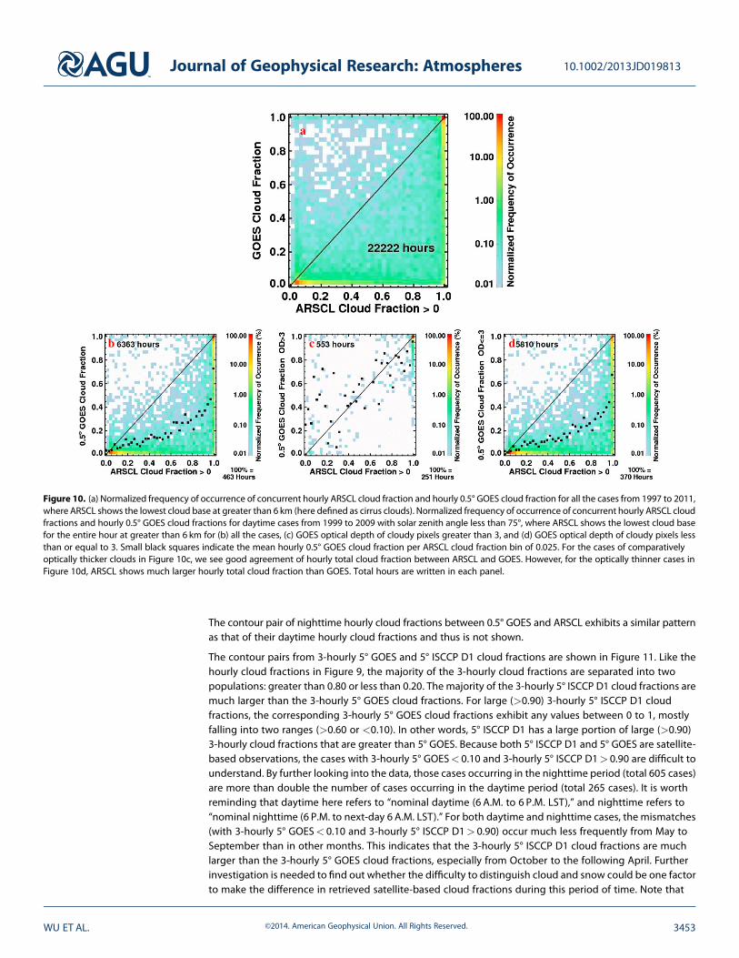
The differences of the cloud fractions between ARSCL and the other estimates shown in Figure 9 are at leastin part because ARSCL cloud fractions are retrieved based on active sensors which can effectively detect highand optically thin cirrus clouds that are not traditionally considered as cloudy sky while TSI, RFA, and 0.5°GOES cloud fractions are all retrieved from passive instruments that categorize high subvisual to translucentcirrus clouds using a more traditional “clear-sky” definition [Dupont et al., 2008]. To illustrate the contributionof these thin cirrus clouds, Figure 10a shows a comparison of cloud fraction estimates from ARSCL and GOESfor all the cases where the lowest cloud base as determined from ARSCL is greater than 6 km (here defined ascirrus clouds). ARSCL almost always shows a larger cloud fraction than GOES. To further support the influenceof thin cirrus on the ARSCL cloud fraction, Figures 10b to 10d compare 1999–2009 cloud fraction estimatesfrom ARSCL and GOES for all the daytime cases (Figure 10b) where the lowest cloud base as determined fromARSCL is greater than 6 km, and then subdivide Figure 10b into cases where the GOES visible optical depth isgreater than three (Figure 10c) and less than three (Figure 10d). Note that the optical depth values are forcloudy sky only, and so, the 0.5° grid box optical depth refers to the mean optical depth for cloudy pixelswithin the grid box. These figures show that for cases of optically thick cirrus, the ARSCL and GOES cloudfractions agree much better in the aggregate average, while for the optically thin cirrus, ARSCL shows aconsistently larger cloud fraction. This is consistent with the statement by Zhao et al. [2012] or Stubenrauchet al. [2013] that the differences in cloud macrophysical properties (cloud fraction here) are rooted in thedifferences in the instrument basis, retrieval methods, and the errors and biases in the measurement inputs.Furthermore, in Figure 9, the correlation coefficients in all the contour pairs are higher than 0.84 for all-skycloud fractions but less than 0.54 for cloud fractions from 0.10 to 0.90. It suggests that all the daytime hourlycloud fractions have a relatively good agreement in their phase variations, but the high correlations betweenthe daytime hourly cloud fractions are driven by the large portion of the near clear-sky (<0.10) and nearovercast (0.90) occurrences.

Figure 9. Joint frequency distributions of concurrent daytime all-sky hourly cloud fractions ((a and b) ARSCL versus TSI/RFAand (c–e) 0.5° GOES versus ARSCL/TSI/RFA). In each panel, a red diagonal line represents a perfect match as a reference, anda correlation coefficient is shown on the bottom right corner. The correlation coefficients without a parenthesis are from all-sky cloud fractions, and those with a parenthesis are from cloud fractions from 0.10 to 0.90.



The contour pair of nighttime hourly cloud fractions between 0.5° GOES and ARSCL exhibits a similar patternas that of their daytime hourly cloud fractions and thus is not shown.

The contour pairs from 3-hourly 5° GOES and 5° ISCCP D1 cloud fractions are shown in Figure 11. Like thehourly cloud fractions in Figure 9, the majority of the 3-hourly cloud fractions are separated into twopopulations: greater than 0.80 or less than 0.20. The majority of the 3-hourly 5° ISCCP D1 cloud fractions aremuch larger than the 3-hourly 5° GOES cloud fractions. For large (>0.90) 3-hourly 5° ISCCP D1 cloudfractions, the corresponding 3-hourly 5° GOES cloud fractions exhibit any values between 0 to 1, mostlyfalling into two ranges (>0.60 or <0.10). In other words, 5° ISCCP D1 has a large portion of large (>0.90)3-hourly cloud fractions that are greater than 5° GOES. Because both 5° ISCCP D1 and 5° GOES are satellite-based observations, the cases with 3-hourly 5° GOES< 0.10 and 3-hourly 5° ISCCP D1> 0.90 are difficult tounderstand. By further looking into the data, those cases occurring in the nighttime period (total 605 cases)are more than double the number of cases occurring in the daytime period (total 265 cases). It is worthreminding that daytime here refers to “nominal daytime (6 A.M. to 6 P.M. LST),” and nighttime refers to“nominal nighttime (6 P.M. to next-day 6 A.M. LST).” For both daytime and nighttime cases, the mismatches(with 3-hourly 5° GOES< 0.10 and 3-hourly 5° ISCCP D1> 0.90) occur much less frequently from May toSeptember than in other months. This indicates that the 3-hourly 5° ISCCP D1 cloud fractions are muchlarger than the 3-hourly 5° GOES cloud fractions, especially from October to the following April. Furtherinvestigation is needed to find out whether the difficulty to distinguish cloud and snow could be one factorto make the difference in retrieved satellite-based cloud fractions during this period of time. Note that

b c d

a

Figure 10. (a) Normalized frequency of occurrence of concurrent hourly ARSCL cloud fraction and hourly 0.5° GOES cloud fraction for all the cases from 1997 to 2011,where ARSCL shows the lowest cloud base at greater than 6 km (here defined as cirrus clouds). Normalized frequency of occurrence of concurrent hourly ARSCL cloudfractions and hourly 0.5° GOES cloud fractions for daytime cases from 1999 to 2009 with solar zenith angle less than 75°, where ARSCL shows the lowest cloud basefor the entire hour at greater than 6 km for (b) all the cases, (c) GOES optical depth of cloudy pixels greater than 3, and (d) GOES optical depth of cloudy pixels lessthan or equal to 3. Small black squares indicate the mean hourly 0.5° GOES cloud fraction per ARSCL cloud fraction bin of 0.025. For the cases of comparativelyoptically thicker clouds in Figure 10c, we see good agreement of hourly total cloud fraction between ARSCL and GOES. However, for the optically thinner cases inFigure 10d, ARSCL shows much larger hourly total cloud fraction than GOES. Total hours are written in each panel.



ISCCP uses a visible and infraredthreshold during the daytime andthen determines a secondaryinfrared-only threshold to matchthe visible and infrared cloudamount during the daytime. Thissecondary infrared-only thresholdis then applied for nighttime toobtain consistent cloud amount.However, the GOES approach usesmultiple infrared channelthresholds for nighttime.

The correlation coefficients in the3-hourly contour pairs are low(0.65 or 0.50 for all-sky daytime ornighttime 3-hourly 5° cloud

fractions, and 0.48 or 0.44 for daytime or nighttime 3-hourly 5° cloud fractions from 0.10 to 0.90), furthersuggesting that the 3-hourly 5° ISCCP D1 and the 3-hourly 5° GOES cloud fractions have a pooragreement in their phase variations.

To illustrate the contribution to the difference of total cloud fraction between GOES and ISCCP,Figures 12a and 12b show a comparison of daytime/nighttime 3-hourly 2.5° equal-area ISCCP D1 and3-hourly 2.5° GOES (taken over the same area as the ISCCP grid box) confirming that ISCCP cloud fractionsare generally larger than GOES. Like the case for 5° ISCCP D1 and 5° GOES (Figure 11), 2.5° equal-areaISCCP D1 shows a large portion of large (>0.90) 3-hourly cloud fractions that are greater than 2.5° GOESwhich is mostly falling into two ranges (>0.80 or<0.10). By further partitioning into cases of predominantlyhigh clouds (c and d) and predominantly low clouds (e and f), it can be seen that ISCCP and GOES agreerelatively well on average for predominantly high clouds, but for predominantly low clouds ISCCP shows amuch larger cloud fraction in general. Note that, “high cloud” is defined as that for which ISCCP infraredcloud top pressure is less than or equal to 440 mbar, as defined by ISCCP. Conversely, “low cloud” isdefined as that for which ISCCP infrared cloud top pressure is greater than 440 mbar. “Predominantly highclouds” means that in the ISCCP profile of cloud fraction, there is at least double the amount of clouds athigh levels (infrared cloud top pressure<= 440 mbar) as there are at low levels (infrared cloud toppressure> 440 mbar). Likewise, “Predominantly low clouds” means that in the ISCCP profile of cloudfraction, there is at least double the amount of clouds at low levels (infrared cloud top pressure> 440 mbar)as there are at high levels (infrared cloud top pressure<= 440 mbar). It is worth mentioning that wetested the sensitivity to the low clouds defined by ISCCP cloud top-pressure threshold and found littleimpact on our results; some (perhaps even many) scenes may include thin cirrus despite ISCCP cloud top-pressure> 440 mbar.

The first step toward investigating the larger cloud fractions reported by ISCCP compared to GOES was tolook for differences between the nominal daytime (6 A.M. to 6 P.M. LST) and nominal nighttime (6 P.M. tonext-day 6 A.M. LST) periods (Figures 11 and 12). For this application, we defined the split between daytime(solar zenith angle (SZA)< 75°) and nighttime (SZA> 100°) so that more precisely taking into accountseasonal variations in the length of the day. This analysis showed that the relationship between 3-hourly 2.5°equal-area ISCCP and 3-hourly 2.5° GOES cloud fractions for the SZA-based daytime case looks similar to thatfor the SZA-based nighttime case with a small difference in between (not shown).

Figure 13 shows an example to illustrate the differences in detecting and defining cloud fractions. On 17December 2007 between approximately 1330 and 1800 UTC, the MMCR detects a thin layer of cirruscloud between 8 km and 10 km (Figure 13a). From the Eulerian view of the MMCR, the observed cloud isvirtually unbroken and the resulting ARSCL cloud fraction is 1 (or nearly so) over this entire period.Coincident images from the TSI at 1424 UTC (Figure 13b) and 1731 UTC (Figure 13d) clearly indicate thepresence of optically thin cirrus clouds that still exhibit a significant blue tint for the sky oriented instreaks (likely contrails). However, the TSI cloud decision algorithm (see section 2.1.2) results (Figures 13c and 13e)

Figure 11. Joint frequency distribution of concurrent daytime (“nominal day-time”, 6 am to 6 pm LST) (a) and nighttime (“nominal nighttime”, 6 pm to next-day 6 am LST) (b) all-sky 3-hourly cloud fractions (5o GOES vs 5o ISCCP D1). Ineach panel, a red diagonal line represents a perfect match as a reference, and acorrelation coefficient is shown on the bottom right corner. The correlationcoefficients without a parenthesis are from all-sky cloud fractions, and thosewith a parenthesis are from cloud fractions from 0.10 to 0.90.



indicate that these thin cirrus clouds are below the set threshold, and therefore, the cloud fractionsestimated from the TSI are 0.01 for a 100° FOV and 0.06 for a 160° FOV at 1424 UTC, and 0.07 for a 100° FOVand 0.18 for a 160° FOV at 1731 UTC. In this case, and for many of the other large discrepancies, a combinationof cloud orientation and morphology, instrument viewing geometry and FOVs, and differences in classificationthresholds results in large differences in cloud fraction estimates and makes the determination of a “bestestimate” difficult.

a

c

e

b

d

f

Figure 12. Normalized frequency of occurrence of concurrent 3-hourly 2.5° GOES cloud fractions and 3-hourly equal-area2.5° ISCCP D1 cloud fractions over the same area with a center at (97.75°W, 36.25°N) from 1999 to 2009. Cases: all (a) daytimeand (b) nighttime cases; (c) daytime and (d) nighttime cases with predominantly high clouds for which there is at least twicethe amount of high cloud as low cloud, that is, total cloud fraction (high cloud)>=2× total cloud fraction (low cloud); and (e)daytime and (f) nighttime cases with predominantly low clouds for which there is at least twice the amount of low cloud ashigh cloud, that is, total cloud fraction (low cloud)>=2× total cloud fraction (high cloud). Here “high cloud” is defined as thatfor which infrared cloud top pressure is less than or equal to 440 mbar, as defined by ISCCP. Conversely, “low cloud” is definedas that for which infrared cloud top pressure is greater than 440 mbar. Small black squares indicate the mean 3-hourly 2.5°GOES total cloud fraction per 3-hourly equal-area 2.5° ISCCP D1 total cloud fraction bin of 0.025. In each panel, the total hours(called “A”) are written in upper left corner, the total hours where the ISCCP total cloud fraction> 0.90 and the GOES totalcloud fraction< 0.10 (called “B”) are written in bottom right corner, and the percentage in bottom right corner refers to B/A.Note that in this figure, daytime and nighttime refer to 6A.M. to 6P.M. local standard time (LST) (“nominal daytime”) and 6P.M.to next-day 6A.M. LST (“nominal nighttime”) as in Figure 11.



5. Summary

This study compares multiscalemean cloud fractions based on1997–2011 observationally basedcloud fraction estimates from sixdifferent platforms over the ARMSGP sites. Three ground-basedestimates (ARSCL, TSI, and RFA) andthree satellite-based estimates(GOES, ISCCP, and PATMOS-x) atmultiple temporal and spatial scalesare examined. Large differences ofcloud fraction between differentestimates are found. In particular,ISCCP and ARSCL are found to havesignificantly larger cloud fractionsthan the rest of the estimates. Threeestimates (ISCCP, ARSCL, and GOES)exhibit an overall increase of 0.08–0.10 in the annually averaged cloudfractions from 1998 to 2009;however, the other three estimates(TSI, RFA, and PATMOS-x) exhibitlittle tendency of cloudinessincrease in the same decade.Furthermore, daily cloud fractionsexhibit frequency distributionsdependent on spatial scales, whichare different from monthly cloudfractions showing quasi-Gaussianfrequency distributions.

It should be recognized, as alreadydiscussed by Stephens [1988] andWiscombe [2005], that cloud fraction

is often determined by a threshold of radiation properties, which in turn is likely dependent on wavelength.As discussed above, the determination of cloud fraction also depends on many other factors including cloudorientation and morphology, and instrumental viewing geometry and FOVs. Thus, different observationallybased cloud fraction estimates may be best for addressing specific issues. For example, ARSCL has a certainadvantage in studying vertical distributions of cloud fraction compared to all other estimates. It is worthmentioning that although ISCCP exhibits much larger total cloud fractions than GOES and PATMOS-x over theSGP site as shown in this paper, the latitudinal variation of total cloud fraction from ISCCP agrees well withthose from 10 other satellite-based total cloud fractions including PATMOS-x [Stubenrauch et al., 2013,Figure 2]. Nevertheless, the existing large differences between cloud fraction estimates suggest a need forfurther investigation into the causes underlying the large differences pertaining to the observationally basedcloud fraction estimates being used in any particular research endeavor. For practical purposes, it isimportant to use a consistent definition of cloud fraction in both climate models and observations, sinceinconsistent definitions of cloud fraction may end up with completely different conclusions as shown in thisstudy. At the very minimum, any activity that professes to produce a value for cloud fraction should also givesome valuation of what limit is used to delineate between cloud and no cloud.

It is also worth emphasizing that the development of consistent and accurate cloud fraction estimates as wellas other cloud properties (e.g., optical thickness) is crucial for climate studies, especially from the perspectiveof the Earth’s radiation budget. As shown in Koren et al. [2007], even a “twilight zone,” a belt around currentlyclassified clouds (with a width of 10 km or more) forming and evaporating cloud fragments and hydrated

Figure 13. An example of cloud observations for December 17, 2007 illustratinga typical case where large discrepancies exist between cloud fraction estimates.(a) ARSCL best estimate radar reflectivity showing cloud fraction 1 at 1424 UTCor 1731 UTC (the dashed lines), where “AGL” refers to “Above Ground Level”,(b) TSI true color image at 1424 UTC, (c) TSI cloud identification at 1424 UTC(cloud fraction = 0.01 for a 100o FOV or 0.06 for a 160o FOV), (d) TSI truecolor image at 1731 UTC, and (e) TSI cloud identification at 1731 UTC (cloudfraction= 0.07 for a 100o FOV or 0.18 for a 160o FOV). The inner circle and thewhole circle represent a 100o FOV and a 160o FOV, respectively.



aerosols, can significantly impact the estimation of the Earth’s radiative forcing. In other words, computingcloud fraction and associated cloud properties over both cloud edges and interior is important fordetermining the Earth’s radiation budget. Of course, because the determination of cloud fraction isdependent on many factors (e.g., wavelength, instrumental viewing geometry and FOVs, etc.), a “cloud-free” atmosphere must be dependent on those factors as well and so does a twilight zone. For making abetter estimation of the Earth’s radiation budget in a cloudy atmosphere, it is necessary to separatelyinvestigate cloudy atmosphere, the twilight zone, and cloud-free atmosphere, as pointed out by Koren et al.[2007] and Bar-Or et al. [2010, 2011]. Further studies are highly suggested on how to consistently defineand determine cloudy atmosphere, the twilight zone, and cloud-free atmosphere in climate models andobservations for better estimating the Earth’s radiation budget.

ReferencesAckerman, T. P., and G. M. Stokes (2003), The atmospheric radiation measurement program, Phys. Today, 56, 38–44, doi:10.1063/1.1554135.Ackerman, S. A., R. E. Holz, R. Frey, E. W. Eloranta, B. C. Maddux, and M. McGill (2008), Cloud detection with MODIS Part II: Validation, J. Atmos.

Oceanic Technol., 25, 1073–1086.Ahlgrimm, M., and M. Köhler (2010), Evaluation of trade cumulus in the ECMWF model with observations from CALIPSO, Mon. Weather Rev.,

138, 3071–3083.Barker, H. W., G. L. Stephens, and Q. Fu (1999), The sensitivity of domain-averaged solar fluxes to assumptions about cloud geometry, Q. J. R.

Meteorol. Soc., 125, 2127–2152.Bar-Or, R. Z., I. Koren, and O. Altaratz (2010), Estimating cloud field coverage using morphological analysis, Environ. Res. Lett., 5, 014022,

doi:10.1088/1748-9326/5/1/014022.Bar-Or, R. Z., O. Altaratz, and I. Koren (2011), Global analysis of cloud field coverage and radiative properties, using morphological methods

and MODIS observations, Atmos. Chem. Phys., 11, 191–200, doi:10.5194/acp-11-191-2011.Bedacht, E., S. K. Gulev, and A. Macke (2007), Intercomparison of global cloud cover fields over oceans from the VOS observations and NCEP/

NCAR reanalysis, Int. J. Climatol., 27, 1707–1719.Bendat, J. S., and A. G. Piersol (1986), Random Data Analysis and Measurement Procedures, 2nd ed., 566 pp., John Wiley, New York.Bender, F. A.-M. (2011), Planetary albedo in strongly forced climate, as simulated by the CMIP3 models, Theor. Appl. Climatol., 105, 529–535,

doi:10.1007/s00704-011-0411-2.Bouniol, D., et al. (2010), Using continuous ground-based radar and lidar measurements for evaluating the representation of clouds in four

operational models, J. Appl. Meteorol. Climatol., 49, 1971–1991.Brooks, M. E., R. J. Hogan, and A. J. Illingworth (2005), Parameterizing the difference in cloud fraction defined by area and by volume as

observed with radar and lidar, J. Atmos. Sci., 62, 2248–2260.Caulcutt, R. (1991), Statistics in Research and Development, 2nd ed., 471 pp., Chapman & Hall, U. K.Clothiaux, E. E., T. P. Ackerman, G. G. Mace, K. P. Moran, R. T. Marchand, M. A. Miller, and B. E. Martner (2000), Objective determination of cloud

heights and radar reflectivities using a combination of active remote sensors at the ARM CART sites, J. Appl. Meteorol., 39, 645–665,doi:10.1175/1520-0450(2000)039<0645:ODOCHA>2.0.CO;2.

Del Genio, A. D., M.-S. Yao, W. Kovari, and K. K. Lo (1996), A prognostic cloud water parameterization for global climate models, J. Clim., 9,270–304, doi:10.1175/1520-0442(1996)009<0270:APCWPF>2.0.CO;2.

Di Girolamo, L., and R. Davies (1997), Cloud fraction errors caused by finite resolution measurements, J. Geophys. Res., 102, 1739–1756,doi:10.1029/96JD02663.

Dupont, J. C., M. Haeffelin, and C. N. Long (2008), Evaluation of cloudless-sky periods detected by shortwave and longwave algorithms usinglidar measurements, Geophys. Res. Lett., 35, L10815, doi:10.1029/2008GL033658.

Evan, A. T., A. K. Heidinger, and D. J. Vimont (2007), Arguments against a physical long-term trend in global ISCCP cloud amounts, Geophys.Res. Lett., 34, L04701, doi:10.1029/2006GL028083.

Evan, A. T., A. K. Heidinger, and Y. Liu (2008), State of the climate in 2007, Bull. Am. Meteorol. Soc., 89, S23–S26.Foster, M. J., and A. K. Heidinger (2013), PATMOS-x: Results from a diurnally corrected thirty-year satellite cloud climatology, J. Clim., 26,

414–425, doi:10.1175/JCLI-D-11-00666.1.Guichard, F., D. B. Parsons, J. Dudhia, and J. Bresch (2003), Evaluating mesoscale model predictions of clouds and radiation with SGP ARM

data over a seasonal timescale, Mon. Weather Rev., 131, 926–944.Heidinger, A., A. T. Evan, M. J. Foster, and A. Walther (2012), A naive Bayesian cloud-detection scheme derived from CALIPSO and applied

within PATMOS-x, J. Appl. Meteorol. Climatol., 51, 1129–1144.Hogan, R. J., and A. J. Illingworth (2000), Deriving cloud overlap statistics from radar, Q. J. R. Meteorol. Soc., 126, 2903–2909.Hogan, R. J., C. Jakob, and A. J. Illingworth (2001), Comparison of ECMWF winter-season cloud fraction with radar-derived values, J. Appl.

Meteorol., 40, 513–525.Jacobowitz, H., L. L. Stowe, G. Ohring, A. Heidinger, K. Knapp, and N. R. Nalli (2003), The Advanced Very High Resolution Radiometer

Pathfinder Atmosphere (PATMOS) climate dataset: A resource for climate research, Bull. Am. Meteorol. Soc., 84, 785–793, doi:10.1175/BAMS-84-6-785.

Jakob, C. (1999), Cloud cover in the ECMWF reanalysis, J. Clim., 12, 947–959.Kassianov, E., C. N. Long, and M. Ovtchinnikov (2005), Cloud sky cover versus cloud fraction: Whole-sky simulations and observations, J. Appl.

Meteorol., 44, 86–98, doi:10.1175/JAM-2184.1.Kato, S., and A. Marshak (2009), Solar zenith and viewing geometry-dependent errors in satellite retrieved cloud optical thickness: Marine

stratocumulus case, J. Geophys. Res., 114, D01202, doi:10.1029/2008JD010579.Kennedy, A. D., X. Dong, B. Xi, S. Xie, Y. Zhang, and J. Chen (2011), A comparison of MERRA and NARR reanalyses with the DOE ARM SGP data,

J. Clim., 24, 4541–4557, doi:10.1175/2011JCLI3978.1.Kennedy, A. D., X. Dong, and B. Xi (2013), Cloud fraction at the ARM SGP site: Instrument and sampling considerations from 14 years of ARSCL,

Theor. Appl. Climatol., doi:10.1007/s00704-013-0853-9.Knapp, K. R. (2008), Calibration assessment of ISCCP geostationary infrared observations using HIRS, J. Atmos. Oceanic Technol., 25, 183–195.

AcknowledgmentsThis work has been supported by theOffice of Biological and EnvironmentalResearch of the U.S. Department ofEnergy as part of the Earth SystemModeling program via the Fast-physicsSystem Testbed and Research (FASTER)project (www.bnl.gov/faster),Atmospheric Radiation Measurementprogram, and Atmospheric SystemsResearch program, the National ClimaticData Center, and the BrookhavenNational Laboratory LaboratoryDirected Research and DevelopmentProgram. Recognition is also extendedto those responsible for the operationand maintenance of the instrumentsthat produced the data used in thisstudy; their diligent and dedicatedefforts are often underappreciated. Wethank Peter H. Daum for carefully read-ing and editing the manuscript andproviding constructive comments, AlanK. Betts, William B. Rossow, Warren J.Wiscombe, and Stephen E. Schwartz forhelpful comments and suggestions. Wealso thank Wuyin Lin, Karen Johnson,Shaocheng Xie, Renata B. McCoy,Mandana Khaiyer, Violeta Golea, andVictor R. Morris for assistance on cloudfraction products used in this study.



http://dx.doi.org/10.1063/1.1554135

http://dx.doi.org/10.1088/1748&hyphen;9326/5/1/014022

http://dx.doi.org/10.5194/acp&hyphen;11&hyphen;191&hyphen;2011

http://dx.doi.org/10.1007/s00704&hyphen;011&hyphen;0411&hyphen;2

http://dx.doi.org/10.1175/1520&hyphen;0450(2000)039<0645:ODOCHA>2.0.CO;2



http://dx.doi.org/10.1175/1520&hyphen;0442(1996)009<0270:APCWPF>2.0.CO;2



http://dx.doi.org/10.1029/96JD02663

http://dx.doi.org/10.1029/2008GL033658

http://dx.doi.org/10.1029/2006GL028083

http://dx.doi.org/10.1175/JCLI&hyphen;D&hyphen;11&hyphen;00666.1

http://dx.doi.org/10.1175/BAMS&hyphen;84&hyphen;6&hyphen;785

http://dx.doi.org/10.1175/BAMS&hyphen;84&hyphen;6&hyphen;785

http://dx.doi.org/10.1175/JAM&hyphen;2184.1

http://dx.doi.org/10.1029/2008JD010579

http://dx.doi.org/10.1175/2011JCLI3978.1

http://dx.doi.org/10.1007/s00704&hyphen;013&hyphen;0853&hyphen;9

www.bnl.gov/faster

Kollias, P., E. E. Clothiaux, B. A. Albrecht, M. A. Miller, K. P. Moran, and K. L. Johnson (2005), The atmospheric radiation measurement program cloudprofiling radars. An evaluation of signal processing and sampling strategies, J. Atmos. Oceanic Technol., 22, 930–948, doi:10.1175/JTECH1749.

Kollias, P., E. E. Clothiaux, M. A. Miller, E. P. Luke, K. L. Johnson, K. P. Moran, K. B. Widener, and B. A. Albrecht (2007a), The atmospheric radiationmeasurement program cloud profiling radars: Second-generation sampling strategies, processing and cloud data products, J. Atmos. Sci.,24, doi:10.1175/JTECH2033.1.

Kollias, P., G. Tselioudis, and B. A. Albrecht (2007b), Cloud climatology at the Southern Great Plains and the layer structure, drizzle, andatmospheric modes of continental stratus, J. Geophys. Res., 112, D09116, doi:10.1029/2006JD007307.

Koren, I., L. A. Remer, Y. J. Kaufman, Y. Rudich, and J. V. Martins (2007), On the twilight zone between clouds and aerosols, Geophys. Res. Lett.,34, L08805, doi:10.1029/2007GL029253.

Liu, Y., W. Wu, M. P. Jensen, and T. Toto (2011), Relationship between cloud radiative forcing, cloud fraction and cloud albedo, and newground-based approach for determining cloud albedo, Atmos. Chem. Phys., 11, 7155–7170, doi:10.5194/acp-11-7155-2011.

Loeb, N. G., B. A. Wielicki, F. G. Rose, and D. R. Doelling (2007), Variability in global top-of-atmosphere shortwave radiation between 2000 and2005, Geophys. Res. Lett., 34, L03704, doi:10.1029/2006GL028196.

Long, C. N. (2010), Correcting for circumsolar and near-horizon errors in sky cover retrievals from sky images, Open Atmos. Sci. J., 4, 45–52.Long, C. N., and T. P. Ackerman (2000), Identification of clear skies from broadband pyranometer measurements and calculation of down-

welling shortwave cloud effects, J. Geophys. Res., 105(D12), 15,609–15,626.Long, C. N., D. W. Slater, and T. Tooman (2001), Total sky imager model 880 status and testing results. ARM Technical Report ARM TR-006, U.S.

Department of Energy, Washington, D. C.Long, C. N., T. P. Ackerman, K. L. Gaustad, and J. N. S. Cole (2006a), Estimation of fractional sky cover from broadband shortwave radiometer

measurements, J. Geophys. Res., 111, D11204, doi:10.1029/2005JD006475.Long, C. N., J. M. Sabburg, J. Calbo, and D. Pages (2006b), Retrieving cloud characteristics from ground-based daytime color all-sky images,

J. Atmos. Oceanic Technol., 23, 633–652.Long, C. N., E. G. Dutton, J. A. Augustine, W. Wiscombe, M. Wild, S. A. McFarlane, and C. J. Flynn (2009), Significant decadal brightening of

downwelling shortwave in the continental US, J. Geophys. Res., 114, D00D06, doi:10.1029/2008JD011263.Mace, G. G., and S. Benson-Troth (2002), Cloud layer overlap characteristics derived from long-term cloud radar data, J. Clim., 15, 2505–2515.Manabe, S., and R. F. Strickler (1964), Thermal equilibrium of the atmosphere with a convective adjustment, J. Atmos. Sci., 21, 361–385,

doi:10.1175/1520-0469(1964)021<0361:TEOTAW>2.0.CO;2.Min, Q., T. Wang, C. N. Long, and M. Duan (2008), Estimating fractional sky cover from spectral measurements, J. Geophys. Res., 113, D20208,

doi:10.1029/2008JD010278.Minnis, P. (1989), Viewing zenith angle dependence of cloudiness determined from coincident GOES East and GOES West data, J. Geophys.

Res., 94, 2303–2320, doi:10.1029/JD094iD02p02303.Minnis, P., et al. (2008), Cloud detection in non-polar regions from CERES using TRMM VIRS and Terra and Aqua MODIS data, IEEE Trans.

Geosci. Remote Sens., 46, 3857–3884.Moran, K. P., B. E. Martner, M. J. Post, R. A. Kropfli, D. C. Welsh, and K. B. Widener (1998), An unattended cloud-profiling radar for use in climate

research, Bull. Am. Meteorol. Soc., 79, 443–455, doi:10.1175/15200477(1998)079<0443:AUCPRF>2.0.CO:2.Morris, V. R. (2005), Total Sky Imager (TSI) handbook, ARM TR-017, June 2005. [Available at http://www.arm.gov/publications/tech_reports/

handbooks/tsi_handbook.pdf.]Park, S., and C. S. Bretherton (2009), The University of Washington shallow convection and moist turbulence schemes and their impact on

climate simulations with the community atmosphere model, J. Clim., 22, 3449–3469, doi:10.1175/2008JCLI2557.1.Qian, Y., C. N. Long, H. Wang, J. M. Comstock, S. A. McFarlane, and S. Xie (2012), Evaluation of cloud fraction and its radiative effect simulated

by IPCC AR4 global models against ARM surface observations, Atmos. Chem. Phys., 12, 1785–1810, doi:10.5194/acp-12-1785-2012.Ramanathan, V., and J. A. Coakley Jr. (1978), Climate modeling through radiative-convective models, Rev. Geophys., 16, 465–489, doi:10.1029/

RG016i004p00465.Rossow, W. B., and L. C. Garder (1993), Validation of ISCCP cloud detections, J. Clim., 6, 2370–2393.Rossow, W. B., and R. A. Schiffer (1999), Advances in understanding clouds from ISCCP, Bull. Am. Meteorol. Soc., 11, 2261–2287.Rossow, W. B., et al. (1985), ISCCP cloud algorithm intercomparison, J. Climate Appl. Meteorol., 24, 877–903.Rossow, W. B., A. W. Walker, and L. C. Garder (1993), Comparison of ISCCP and other cloud amounts, J. Clim., 6, 2394–2418.Rossow, W. B., A. W. Walker, D. Beuschel, and M. Roiter (1996), International Satellite Cloud Climatology Project (ISCCP) documentation of

new cloud datasets, WMO/TD-No. 737, World Meteorological Organization, 115 pp.Slingo, A., R. C. Wilderspin, and R. N. B. Smith (1989), Effect of improved physical parameterizations on simulations of cloudiness and the

Earth’s radiation budget, J. Geophys. Res., 94, 2281–2301, doi:10.1029/JD094iD02p02281.Smith, R. N. B. (1990), A scheme for predicting layer clouds and their water content in a general circulation model, Q. J. R. Meteorol. Soc., 116,

435–460, doi:10.1002/qj.49711649210.Sokolov, A. P., and E. Monier (2012), Changing the climate sensitivity of an atmospheric general circulation model through cloud radiative

adjustment, J. Clim., 25, 6567–6584, doi:10.1175/JCLI-D-11-00590.1.Spinhurne, J. D. (1993), Micro pulse lidar, IEEE Trans. Geosci. Remote Sens., 31, 48–55.Stephens, G. L. (1988), Radiative transfer through arbitrary shaped optical media, II: Group theory and simple closures, J. Atmos. Sci., 45, 1837–1848.Stokes, G. M., and S. E. Schwartz (1994), The Atmospheric Radiation Measurement (ARM) program: Programmatic background and design of

the cloud and radiation test bed, Bull. Am. Meteorol. Soc., 75, 1201–1221.Stowe, L. L., H. Jacobowitz, G. Ohring, K. R. Knapp, and N. R. Nalli (2002), The Advanced Very High Resolution Radiometer (AVHRR) Pathfinder

Atmosphere (PATMOS) climate dataset: Initial analyses and evaluations, J. Clim., 15, 1243–1260.Stubenrauch, C., et al. (2013), Assessment of global cloud datasets from satellites: Project and database initiated by the GEWEX Radiation

Panel, Bull. Am. Meteorol. Soc., 94, 1031–1049, doi:10.1175/BAMS-D-12-00117.Sundqvist, H., E. Berge, and J. E. Kristjánsson (1989), Condensation and cloud parameterization studies with a mesoscale numerical weather

prediction model, Mon. Weather Rev., 117, 1641–1657, doi:10.1175/1520-0493(1989)117<1641:CACPSW>2.0.CO;2.Tiedtke, M. (1993), Representation of clouds in large-scale models, Mon. Weather Rev., 121, 3040–3061, doi:10.1175/1520-0493(1993)

121<3040:ROCILS>2.0.CO;2.Turner, D. D., S. A. Clough, J. C. Liljegren, E. E. Clothiaux, K. Cady-Pereira, and K. L. Gaustad (2007), Retrieving liquid water path and precipitable

water vapor from Atmospheric Radiation Measurement (ARM) microwave radiometers, IEEE Trans. Geosci. Remote Sens., 45, 3680–3690,doi:10.1109/TGRS.2007.903703.

Walsh, J. E., W. L. Chapman, and D. H. Portis (2009), Arctic cloud fraction and radiative fluxes in atmospheric reanalyses, J. Clim., 22, 2316–2334,doi:10.1175/2008JCLI2213.1.



http://dx.doi.org/10.1175/JTECH1749

http://dx.doi.org/10.1175/JTECH2033.1

http://dx.doi.org/10.1029/2006JD007307

http://dx.doi.org/10.1029/2007GL029253


http://dx.doi.org/10.1029/2006GL028196

http://dx.doi.org/10.1029/2005JD006475

http://dx.doi.org/10.1029/2008JD011263

http://dx.doi.org/10.1175/1520&hyphen;0469(1964)021<0361:TEOTAW>2.0.CO;2



http://dx.doi.org/10.1029/2008JD010278

http://dx.doi.org/10.1029/JD094iD02p02303

http://dx.doi.org/10.1175/15200477(1998)079<0443:AUCPRF>2.0.CO:2



http://www.arm.gov/publications/tech_reports/handbooks/tsi_handbook.pdf

http://www.arm.gov/publications/tech_reports/handbooks/tsi_handbook.pdf



http://dx.doi.org/10.1029/RG016i004p00465

http://dx.doi.org/10.1029/RG016i004p00465

http://dx.doi.org/10.1029/JD094iD02p02281

http://dx.doi.org/10.1002/qj.49711649210

http://dx.doi.org/10.1175/JCLI&hyphen;D&hyphen;11&hyphen;00590.1

http://dx.doi.org/10.1175/BAMS&hyphen;D&hyphen;12&hyphen;00117

http://dx.doi.org/10.1175/1520&hyphen;0493(1989)117<1641:CACPSW>2.0.CO;2



http://dx.doi.org/10.1175/1520&hyphen;0493(1993)121<3040:ROCILS>2.0.CO;2




http://dx.doi.org/10.1109/TGRS.2007.903703


Warren, S. G., R. M. Eastman, and C. J. Hahn (2007), A survey of changes in cloud cover and cloud types over land from surface observations,1971–96, J. Clim., 20, 717–738, doi:10.1175/JCLI4031.1.

Wielicki, B. A., and L. Parker (1992), On the determination of cloud cover from satellite sensors: The effect of sensor spatial resolution,J. Geophys. Res., 97, 12,799–12,823, doi:10.1029/92JD01061.

Wielicki, B. A., et al. (2002), Evidence for large decadal variability in the tropical mean radiative energy budget, Science, 295, 841, doi:10.1126/science.1065837.

Wilkinson, J. M., R. J. Hogan, A. J. Illingworth, and A. Benedetti (2008), Use of a lidar forward model for global comparisons of cloud fractionbetween the ICESat lidar and the ECMWF model, Mon. Weather Rev., 136, 3742–3759.

Wiscombe, W. J. (2005), Part I (1) (Pages 3 to 92) in 3D Radiative Transfer in Cloudy Atmospheres, edited by A. Marshak and A. B. Davis, pp. 686,Springer, New York.

Wu, W., Y. Liu, and A. K. Betts (2012), Observationally based evaluation of NWP reanalyses in modeling cloud properties over the SouthernGreat Plains, J. Geophys. Res., 117, D12202, doi:10.1029/2011JD016971.

Xi, B., X. Dong, P. Minnis, and M. M. Khaiyer (2010), A 10 year climatology of cloud fraction and vertical distribution derived from both surfaceand GOES observations over the DOE ARM SPG site, J. Geophys. Res., 115, D12124, doi:10.1029/2009JD012800.

Xie, S., et al. (2010), CLOUDS AND MORE: ARM climate modeling best estimate data, Bull. Am. Meteorol. Soc., 91, 13–20, doi:10.1175/2009BAMS2891.1.

Xie, S., X. Liu, C. Zhao, and Y. Zhang (2013), Sensitivity of CAM5-simulated Arctic clouds and radiation to ice nucleation parameterization,J. Clim., 26, 5981–5999.

Yi, H. Y., P. Minnis, L. Nguyen, and D. R. Doelling (2001), A proposed multiangle satellite dataset using GEO, LEO and TRIANA, paper presentedat 11th Conference on Satellite Meteorology and Oceanography (570-573), Am. Meteorol. Soc., Madison, Wisconsin, 12–16 Oct.[Available at http://www-pm.larc.nasa.gov/triana/documents/helen_ams2001.pdf.]

Yu, F., X. Wu, M. K. R. V. Raja, Y. Li, L. Wang, and M. D. Goldberg (2013), Diurnal and scan angle variations in the calibration of GOES imagerinfrared channels, IEEE Trans. Geosci. Remote Sens., 51(1), Jan. 2013. [Available at http://ieeexplore.ieee.org/stamp/stamp.jsp?tp=&arnumber=6215039.]

Zhao, C., et al. (2012), Toward understanding of differences in current cloud retrievals of ARM ground-based measurements, J. Geophys. Res.,117, D10206, doi:10.1029/2011JD016792.

Zuidema, P., and D. L. Hartmann (1995), Satellite determination of stratus cloud microphysical properties, J. Clim., 8, 1638–1656, doi:10.1175/1520-0442(1995)008<1638:SDOSCM>2.0.CO;2.



http://dx.doi.org/10.1175/JCLI4031.1

http://dx.doi.org/10.1029/92JD01061

http://dx.doi.org/10.1126/science.1065837

http://dx.doi.org/10.1126/science.1065837

http://dx.doi.org/10.1029/2011JD016971

http://dx.doi.org/10.1029/2009JD012800

http://dx.doi.org/10.1175/2009BAMS2891.1

http://dx.doi.org/10.1175/2009BAMS2891.1

http://www-pm.larc.nasa.gov/triana/documents/helen_ams2001.pdf

http://ieeexplore.ieee.org/stamp/stamp.jsp?tp=&arnumber=6215039

http://ieeexplore.ieee.org/stamp/stamp.jsp?tp=&arnumber=6215039

http://dx.doi.org/10.1029/2011JD016792

http://dx.doi.org/10.1175/1520&hyphen;0442(1995)008<1638:SDOSCM>2.0.CO;2




A comparison of multiscale variations of decadelong … ceilometersare ground-basedoptical remote...

Documents

Transcript of A comparison of multiscale variations of decadelong … ceilometersare ground-basedoptical remote...