A Collaborative Adaptive Wiener Filter for Image ...

University of DaytoneCommonsElectrical and Computer Engineering FacultyPublications

Department of Electrical and ComputerEngineering

1-2015

A Collaborative Adaptive Wiener Filter for ImageRestoration Using a Spatial-Domain Multi-patchCorrelation ModelKhaled M. MohamedUniversity of Dayton

Russell C. HardieUniversity of Dayton, [email protected]

Follow this and additional works at: https://ecommons.udayton.edu/ece_fac_pub

Part of the Electrical and Electronics Commons, and the Signal Processing Commons

This Article is brought to you for free and open access by the Department of Electrical and Computer Engineering at eCommons. It has been acceptedfor inclusion in Electrical and Computer Engineering Faculty Publications by an authorized administrator of eCommons. For more information, pleasecontact [email protected], [email protected].

eCommons CitationMohamed, Khaled M. and Hardie, Russell C., "A Collaborative Adaptive Wiener Filter for Image Restoration Using a Spatial-DomainMulti-patch Correlation Model" (2015). Electrical and Computer Engineering Faculty Publications. 13.https://ecommons.udayton.edu/ece_fac_pub/13

https://ecommons.udayton.edu?utm_source=ecommons.udayton.edu%2Fece_fac_pub%2F13&utm_medium=PDF&utm_campaign=PDFCoverPages

https://ecommons.udayton.edu/ece_fac_pub?utm_source=ecommons.udayton.edu%2Fece_fac_pub%2F13&utm_medium=PDF&utm_campaign=PDFCoverPages


https://ecommons.udayton.edu/ece?utm_source=ecommons.udayton.edu%2Fece_fac_pub%2F13&utm_medium=PDF&utm_campaign=PDFCoverPages

https://ecommons.udayton.edu/ece?utm_source=ecommons.udayton.edu%2Fece_fac_pub%2F13&utm_medium=PDF&utm_campaign=PDFCoverPages


http://network.bepress.com/hgg/discipline/270?utm_source=ecommons.udayton.edu%2Fece_fac_pub%2F13&utm_medium=PDF&utm_campaign=PDFCoverPages

http://network.bepress.com/hgg/discipline/275?utm_source=ecommons.udayton.edu%2Fece_fac_pub%2F13&utm_medium=PDF&utm_campaign=PDFCoverPages

https://ecommons.udayton.edu/ece_fac_pub/13?utm_source=ecommons.udayton.edu%2Fece_fac_pub%2F13&utm_medium=PDF&utm_campaign=PDFCoverPages

mailto:[email protected],%[email protected]

Mohamed and Hardie EURASIP Journal on Advances in SignalProcessing (2015) 2015:6 DOI 10.1186/s13634-014-0189-3

RESEARCH Open Access

A collaborative adaptive Wiener filter forimage restoration using a spatial-domainmulti-patch correlation modelKhaled M Mohamed† and Russell C Hardie* †

Abstract

We present a new patch-based image restoration algorithm using an adaptive Wiener filter (AWF) with a novelspatial-domain multi-patch correlation model. The new filter structure is referred to as a collaborative adaptive Wienerfilter (CAWF). The CAWF employs a finite size moving window. At each position, the current observation windowrepresents the reference patch. We identify the most similar patches in the image within a given search windowabout the reference patch. A single-stage weighted sum of all of the pixels in the similar patches is used to estimatethe center pixel in the reference patch. The weights are based on a new multi-patch correlation model that takes intoaccount each pixel’s spatial distance to the center of its corresponding patch, as well as the intensity vector distancesamong the similar patches. One key advantage of the CAWF approach, compared with many other patch-basedalgorithms, is that it can jointly handle blur and noise. Furthermore, it can also readily treat spatially varying signal andnoise statistics. To the best of our knowledge, this is the first multi-patch algorithm to use a single spatial-domainweighted sum of all pixels within multiple similar patches to form its estimate and the first to use a spatial-domainmulti-patch correlation model to determine the weights. The experimental results presented show that the proposedmethod delivers high performance in image restoration in a variety of scenarios.

Keywords: Image restoration; Wiener filter; Correlation model; Patch-based processing

1 Introduction1.1 Image restorationDuring image acquisition, images are subject to a varietyof degradations. These invariably include blurring fromdiffraction and noise from a variety of sources. Restoringsuch degraded images is a fundamental problem in imageprocessing that has been researched since the earliest daysof digital images [1,2]. A wide variety of linear and non-linear methods have been proposed. Many methods havefocused exclusively on noise reduction, and others seekto address multiple degradations jointly, such as blur andnoise.A widely used method for image restoration, relevant

to the current paper, is the classic Wiener filter [3].The standard Wiener filter is a linear space-invariantfilter designed to minimize mean squared error (MSE)

*Correspondence: [email protected]†Equal contributorsUniversity of Dayton, Department of Electrical and Computer Engineering, 300College Park, Dayton, 45469-0226 OH, USA

between the desired signal and estimate, assuming sta-tionary random signals and noise. It is important to notethat there are many disparate variations of Wiener filters.These include finite impulse response, infinite impulseresponse, transform-domain, and spatially adaptive meth-ods. Within each of these categories, a wide variety of sta-tistical models may be employed. Some statistical modelsare very simple, such as the popular constant noise-to-signal power spectral density model, and others are farmore complex. In the case of the empirical Wiener filter[4], no explicit statistical model is used at all. Rather, apilot or prototype estimate is used in lieu of a parametricstatistical model.While all of thesemethodsmay go by thename of ‘Wiener filter’, they can be quite different in theircharacter.Recently, a form of adaptive Wiener filter (AWF)

has been developed and successfully applied to super-resolution (SR) and other restoration applications by oneof the current authors [5]. This AWF approach employsa spatially varying weighted sum to form an estimate of

© 2015 Mohamed and Hardie; licensee Springer. This is an Open Access article distributed under the terms of the CreativeCommons Attribution License (http://creativecommons.org/licenses/by/4.0), which permits unrestricted use, distribution, andreproduction in any medium, provided the original work is properly credited.

[email protected]

http://creativecommons.org/licenses/by/4.0

Mohamed and Hardie EURASIP Journal on Advances in Signal Processing (2015) 2015:6 Page 2 of 23

each pixel. The Wiener weights are determined basedon a spatially varying spatial-domain parametric correla-tion model. This particular brand of AWF SR emergedfrom earlier work, including that in [6-8]. This kind ofAWF is capable of jointly addressing blur, noise, andundersampling and is well suited to dealing with a non-stationary signal and noise. The approach is also very wellsuited to dealing with non-uniformly sampled imageryand missing or bad pixels. This AWF SR method has beenshown to provide best-in-class performance for nonuni-form interpolation-based SR [5,9-11] and has also beenused successfully for demosaicing [12,13] and Nyquistsampled video restoration [14]. Under certain conditions,the method can also be very computationally efficient [5].The key to this method lies in the particular correlationmodel used and how it is employed for spatially adaptivefiltering.A different approach to image restoration, also relevant

to the current paper, is based on fusing multiple simi-lar patches within the observed image. This patch-basedapproach is used primarily for noise reduction applica-tions and exploits spatial redundancy that may expressitself within an image, locally and/or non-locally. Themethod of non-local means (NLM), introduced in [15],may be the first method to directly fuse non-local patchesfrom within the observed image based on vector distancesfor the purpose of image denoising. A notable early pre-cursor to the NLM is the vector detection method [16,17].In the vector detection approach, a codebook of repre-sentative patches from training data is used, rather thanpatches from the observed image itself [16,17]. A numberof NLM variations have been proposed, including [18-26].The basic NLM method forms an estimate of a referencepixel as a weighted sum of non-local pixels. The weightsare based on the vector distances of the patch intensi-ties between various non-local patches and the referencepatch. In particular, the center samples of a non-localpatches are weighted in proportion to the negative expo-nential of the corresponding patch distance. The NLMalgorithm can be viewed as an extension of the bilateralfilter [27-31], which forms an estimate by weighting neigh-boring pixels based on both spatial proximity and intensitysimilarity of individual pixels (rather than patches).Improved performance for noise reduction is obtained

with the block matching and 3D filtering (BM3D)approach proposed in [32-34]. The BM3D method alsouses vector distances between patches, but the filter-ing is performed using a transform-domain shrinkageoperation. By utilizing all of the samples within selectedpatches and aggregating the results, excellent noise reduc-tion performance can be achieved with BM3D. Anotherrelated patch-based image denoising algorithm is the totalleast squares method presented in [35]. In this method,each ideal patch is modeled as a linear combination of

similar patches from the observed image. Another typeof patch-based Wiener denoising filter is proposed in[36], and a globalized approach to patch-based denois-ing is proposed in [37]. While such patch-based methodsperform well in noise reduction, most are not capa-ble of addressing blur and noise jointly. However, thereare a few recent methods that do treat both blur andnoise and incorporate multi-patch fusion. These includeBM3D deblurring (BM3DDEB) [38] and iterative decou-pled deblurring-BM3D (IDD-BM3D) [39]. The deblurringin these algorithms is not achieved by patch fusion alone.Rather, the patch fusion component of these algorithmsserves as a type of signal model used for regularization.Note that multi-patch methods have also been developedand applied to SR [40-45]. However, the focus of this paperis on image restoration without undersampling/aliasing.

1.2 Proposedmethod and novel contributionIn this paper, we propose a novel multi-patch AWF algo-rithm for image restoration. In the spirit of [32], we referto this new filter structure as a collaborative adaptiveWiener filter (CAWF). It can be viewed as an exten-sion of the AWF in [5], with the powerful new featureof incorporating multiple patches for each pixel estimate.As with other patch-based algorithms, we employ a mov-ing window. At each position, the current observationwindow represents the reference patch. Within a givensearch window about the reference, we identify the mostsimilar patches to the reference patch. However, insteadof simply weighting just the center pixels of these sim-ilar patches, as with NLM, or using transform-domainshrinkage like BM3D, we use a spatial-domain weightedsum of all of the pixels within all of the selected patchesto estimate the one center pixel in the reference patch.The weights used are based on a novel spatially vary-ing spatial-domain multi-patch correlation model. Thecorrelation model takes into account each pixel’s spatialdistance to the center of its corresponding patch, as well asthe intensity vector distances among the similar patches.The ‘collaborative’ nature of the CAWF springs from thefusion of multiple, potentially non-local, patches. One keyadvantage of the CAWF approach is that it can jointlyhandle blur and noise. Furthermore, the CAWF methodis able to accommodate spatially varying signal and noisestatistics.Our approach is novel in that we use a single-pass

spatial-domain weighted sum of all pixels within all of thesimilar patches to form the estimate each desired pixel.In the case of NLM, only the center pixel of each simi-lar patch is given a weight [15].This is simple and effectivefor denoising, but deconvolution is not possible within thebasic NLM framework, and all of the available informa-tion in the patches may not be exploited. While BM3Ddoes fuse all of the pixels in the similar patches, the fusion


in BM3D is based on a wavelet shrinkage operation andnot a spatial-domain correlation model [32]. Because ofthe nature of wavelet shrinkage, the standard BM3D is alsounable to perform deblurring [32]. On the other hand, theCAWF structure can jointly address blur and noise anddoes not employ separate transform-domain inverse fil-tering as in [38] or iterative processing like that in [39].To the best of our knowledge, this is the first multi-patch algorithm to use a single-pass weighted sum of allpixels within multiple similar patches to jointly addressblur and noise. It is also the first to use a spatial-domainmulti-patch correlation model.The remainder of this paper is organized as follows. The

observation model is described in Section 2. The CAWFalgorithm is presented in Section 3. This includes the basicalgorithm description as well as the new spatial-domainmulti-patch correlation model. Computational complex-ity and implementation are also discussed in Section 3.Experimental results for simulated and real data are pre-sented and discussed in Section 4. Finally, conclusions areoffered in Section 5.

2 ObservationmodelThe proposed CAWF algorithm is based on the observa-tionmodel shown in Figure 1. Themodel input is a desired2D discrete grayscale image, denoted d(n1, n2), wheren1, n2 are the spatial pixel indices. Using lexicographicalnotation, we shall represent all of the pixels in this desiredimage with a single column vector d = [ d1, d2, . . . , dN ]T ,where N is the total number of pixels in the image. Nextin the observation model, we assume the desired imageis convolved with a specified point spread function (PSF),yielding

f (n1, n2) = d(n1, n2) ∗ h(n1, n2), (1)

where h(n1, n2) is the PSF, and ∗ is 2D spatial convolution.In matrix form, this can be expressed as

f = Hd = [ f1, f2, . . . , fN ]T , (2)

where H is an N × N matrix containing values of PSF,and the vector f is the image f (n1, n2) in lexicographicalform. The PSF can be designed to model different types ofblurring, such as diffraction from optics, spatial detection

Figure 1 Observation model block diagram.

integration, atmospheric effects, and motion blurring. Inthe experimental results presented in this paper, we use asimple Gaussian PSF.With regard to noise, our model assumes zero-mean

additive Gaussian noise, with noise standard deviation ofση. Thus, the observed image is given by

g(n1, n2) = f (n1, n2) + η(n1, n2), (3)

where η(n1, n2) is a Gaussian noise array. In lexicographicform, this is given by

g = f + η, (4)

where g =[ g1, g2, . . . , gN ]T and η = [η1, η2, . . . , ηN ]Tare the observed image and noise vectors, respectively.The random noise vector is Gaussian such that η ∼N(0, σ 2

η I).

3 Collaborative adaptiveWiener filter3.1 CAWF overviewThe CAWF employs a moving window approach with amoving reference patch and correspondingmoving searchwindow, each centered about pixel i, where i = 1, 2, . . . ,N .The reference patch spans K1 × K2 = K pixels sym-metrically about pixel i. All of the pixels that lie withinthe span of this reference patch are placed into the ref-erence patch vector defined as gi =[ gi,1, gi,2, . . . , gi,K ]T .The search window is of size L1 × L2 = L pixels. Let theset Si =[ Si(1), Si(2), . . . Si(L)]T contain the indices of thepixels within the search window.The next step in the CAWF algorithm is identifying the

M patches from the search window that are most simi-lar to the reference. This is done using a simple squaredEuclidean distance. That is, we compute

∥∥gi − gj∥∥22, for

j ∈ Si. We select the M patches corresponding to the Msmallest distances and designate these as ‘similar patches’.All of the pixels from the similar patches shall be con-catenated into a single KM × 1 column vector, gi =[gTsi,1 , g

Tsi,2 , . . . , g

Tsi,M

]T, where si = [

si,1, si,2, . . . si,M]T con-

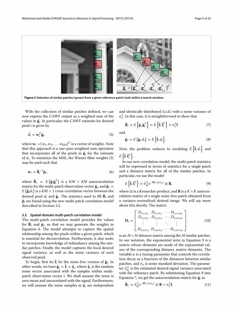
tains the indices of the similar patches in order fromsmallest corresponding distance to largest. The minimumdistance will always be zero and will correspond to the ref-erence patch itself, such that si,1 = i. This selection of sim-ilar patches is common to many patch-based algorithms,such as those in [32-34]. Examples of the similar patchselection is illustrated in Figure 2. The red square repre-sents the reference patch, and the green squares representselected similar patches. Note that there will generally bevariability with regard to how similar the selected patchesare to the reference and to each other. Some referencepatches will have numerous low distance similar patches,and others will not. It is this variability that we wish tocapture and account for with our multi-patch correlationmodel in Section 3.2.


Figure 2 Selection of similar patches (green) from a given reference patch (red) within a search window.

With the collection of similar patches defined, we cannow express the CAWF output as a weighted sum of thevalues in gi. In particular, the CAWF estimate for desiredpixel i is given by

di = wTi gi, (5)

wherewi =[w1,w2, . . . wKM]T is a vector of weights. Notethat this approach is a one-pass weighted-sum operationthat incorporates all of the pixels in gi for the estimateof di. To minimize the MSE, the Wiener filter weights [5]may be used such that

wi = R−1i pi, (6)

where Ri = E{gigTi

}is a KM × KM autocorrelation

matrix for the multi-patch observation vector gi, and pi =E{gidi}is a KM × 1 cross-correlation vector between the

desired pixel di and gi. The statistics used to fill Ri andpi are found using the new multi-patch correlation modeldescribed in Section 3.2.

3.2 Spatial-domain multi-patch correlation modelThe multi-patch correlation model provides the valuesfor Ri and pi, so that we may generate the weights inEquation 6. The model attempts to capture the spatialrelationship among the pixels within a given patch, whichis essential for deconvolution. Furthermore, it also seeksto incorporate knowledge of redundancy among the sim-ilar patches. Finally, the model captures the local desiredsignal variance, as well as the noise variance of eachobserved pixel.To begin, first let fi be the noise-free version of gi. In

other words, we have gi = fi + ηi, where ηi is the randomnoise vector associated with the samples within multi-patch observation vector i. We shall assume the noise iszero mean and uncorrelated with the signal. Furthermore,we will assume the noise samples in ηi are independent

and identically distributed (i.i.d.) with a noise variance ofσ 2

η . In this case, it is straightforward to show that

Ri = E{g igTi

}= E

{fi fTi

}+ σ 2

η I (7)

and

pi = E{gi di

} = E{fi di}. (8)

Now, the problem reduces to modeling E{fi di}

and

E{fi fTi

}.

In our new correlation model, the multi-patch statisticswill be expressed in terms of statistics for a single patchand a distance matrix for all of the similar patches. Inparticular, we use the model

E{fi fTi

}= σ 2

die−Di/(αση) ⊗ R, (9)

where⊗ is a Kronecker product, andR is a K×K autocor-relation matrix of a single noise-free patch obtained froma variance-normalized desired image. We will say moreabout this shortly. The matrix

Di =

⎡⎢⎢⎢⎣

Dsi,1,si,1 Dsi,1,si,2 · · · Dsi,1,si,MDsi,2,si,1 Dsi,2,si,2 · · · Dsi,2,si,M

......

. . ....

Dsi,M ,si,1 Dsi,M ,si,2 · · · Dsi,M ,si,M

⎤⎥⎥⎥⎦ . (10)

is anM×M distance matrix among theM similar patches.In our notation, the exponential term in Equation 9 is amatrix whose elements are made of the exponential val-ues of the corresponding distance matrix elements. Thevariable α is a tuning parameter that controls the correla-tion decay as a function of the distances between similarpatches, and ση is noise standard deviation. The parame-ter σ 2

di is the estimated desired signal variance associatedwith the reference patch. By substituting Equation 9 intoEquation 7, we get the autocorrelation matrix for gi as

Ri = σ 2die

−Di/(αση) ⊗ R + σ 2η I. (11)


In a similar manner, wemodel the cross-correlation vectoras

pi = E{fi di}

= σ 2die

−[Di]1/(αση) ⊗ p, (12)

where p is the K × 1 cross-correlation vector for a singlenormalized patch, and [Di]1 is the first column of the dis-tance matrix Di. The correlation models in Equations 11and 12 capture the spatial correlations among pixelswithin each patch using R and p. The patch similarities,captured in the distance matrix, are used to ‘modulate’these correlations with the Kronecker product to providethe full multi-patch correlation model. In this manner,pixels belonging to patches with smaller inter-patch dis-tances will be modeled with higher correlations amongthem. Potential changes in the underlying desired imagevariance are captured in the model with the term σ 2

di . Inaddition, a spatially varying noise variance can easily beincorporated if appropriate.The specific distance metric used to populate the dis-

tance matrix Di here is a scaled and shifted l2-norm.This type of metric has been used successfully to quantifysimilarity between image patches corrupted with additiveGaussian noise [15]. In particular, the distance betweenpatches centered about pixels i and j is given by

Di,j ={ ‖gi−gj‖2

ση

√2K

− D0‖gi−gj‖2ση

√2K

> D0

0 otherwise(13)

where∥∥gi − gj

∥∥2 is the l

2-norm distance, K is total num-ber of pixels in each patch, and ση is noise standarddeviation. The scaling by ση

√2K normalizes the distance

with respect to K and ση, and D0 can be used as a tuningparameter in the correlation model to adjust for distancedue to noise. To see how the scaling works, and under-stand the potential role of D0, consider the distance withD0 = 0 defined as

Di,j =∥∥gi − gj

∥∥2

ση

√2K

. (14)

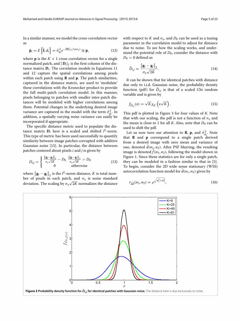
It can be shown that for identical patches with distancedue only to i.i.d. Gaussian noise, the probability densityfunction (pdf) for Di,j is that of a scaled Chi randomvariable and is given by

fDi,j(x) = √KχK

(x√K). (15)

This pdf is plotted in Figure 3 for four values of K. Notethat with our scaling, the pdf is not a function of ση andthe mean is close to 1 for all K. Also, note that D0 can beused to shift the pdf.Let us now turn our attention to R, p, and σ 2

di . Notethat R and p correspond to a single patch derivedfrom a desired image with zero mean and variance ofone, denoted d(n1, n2). After PSF blurring, the resultingimage is denoted f (n1, n2), following the model shown inFigure 1. Since these statistics are for only a single patch,they can be modeled in a fashion similar to that in [5].To begin, consider the 2D wide sense stationary (WSS)autocorrelation function model for d(n1, n2) given by

rdd(n1, n2) = ρ

√n21+n22 , (16)

Figure 3 Probability density function for Di,j for identical patches with Gaussian noise. The distance here is due exclusively to noise.


where ρ is the one pixel step correlation value. The crosscorrelation function between d(n1, n2) and f (n1, n2) canthen be expressed as

rdf (n1, n2) = rdd(n1, n2) ∗ h(n1, n2). (17)

The auto-correlation function for f (n1, n2) can also beexpressed in terms of the desired autocorrelation functionas

rf f (n1, n2) = rdd(n1, n2)∗h(n1, n2)∗h(−n1,−n2). (18)

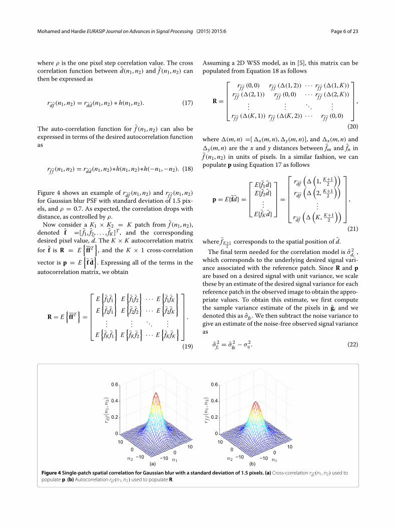
Figure 4 shows an example of rdf (n1, n2) and rf f (n1, n2)for Gaussian blur PSF with standard deviation of 1.5 pix-els, and ρ = 0.7. As expected, the correlation drops withdistance, as controlled by ρ.Now consider a K1 × K2 = K patch from f (n1, n2),

denoted f =[ f1, f2, . . . , fK ]T , and the correspondingdesired pixel value, d. The K × K autocorrelation matrixfor f is R = E

{ffT}, and the K × 1 cross-correlation

vector is p = E{f d}. Expressing all of the terms in the

autocorrelation matrix, we obtain

R = E{ffT}

=

⎡⎢⎢⎢⎢⎢⎢⎣

E{f1 f1}

E{f1 f2}

· · · E{f1 fK}

E{f2 f1}

E{f2 f2}

· · · E{f2 fK}

......

. . ....

E{fK f1}E{fK f2}

· · · E{fK fK

}

⎤⎥⎥⎥⎥⎥⎥⎦.

(19)

Assuming a 2D WSS model, as in [5], this matrix can bepopulated from Equation 18 as follows

R =

⎡⎢⎢⎢⎢⎣

rf f (0, 0) rf f (�(1, 2)) · · · rf f (�(1,K))

rf f (�(2, 1)) rf f (0, 0) · · · rf f (�(2,K))

......

. . ....

rf f (�(K , 1)) rf f (�(K , 2)) · · · rf f (0, 0)

⎤⎥⎥⎥⎥⎦ ,

(20)

where �(m, n) =[�x(m, n),�y(m, n)], and �x(m, n) and�y(m, n) are the x and y distances between fm and fn inf (n1, n2) in units of pixels. In a similar fashion, we canpopulate p using Equation 17 as follows

p = E{fd} =

⎡⎢⎢⎢⎣

E{f1d}E{f2d}

...E{fK d}

⎤⎥⎥⎥⎦ =

⎡⎢⎢⎢⎢⎢⎢⎣

rdf(�(1, K+1

2

))rdf(�(2, K+1

2

))...

rdf(�(K , K+1

2

))

⎤⎥⎥⎥⎥⎥⎥⎦,

(21)

where f K+12

corresponds to the spatial position of d.The final term needed for the correlation model is σ 2

di ,which corresponds to the underlying desired signal vari-ance associated with the reference patch. Since R and pare based on a desired signal with unit variance, we scalethese by an estimate of the desired signal variance for eachreference patch in the observed image to obtain the appro-priate values. To obtain this estimate, we first computethe sample variance estimate of the pixels in gi and wedenoted this as σgi . We then subtract the noise variance togive an estimate of the noise-free observed signal varianceas

σ 2fi = σ 2

gi − σ 2η . (22)

Figure 4 Single-patch spatial correlation for Gaussian blur with a standard deviation of 1.5 pixels. (a) Cross-correlation rdf (n1, n2) used topopulate p. (b) Autocorrelation rf f (n1, n2) used to populate R.


Note that in practice, we do not allow the value inEquation 22 to go below a specifiedminimum value. UsingEquation 17, it can be shown that the relationship betweenσ 2di and σ 2

fi is given by [5]

σ 2di = 1

C(ρ)σ 2fi , (23)

where

C(ρ) =∞∑

−∞

∞∑−∞

ρ

√n21+n22 h(n1, n2), (24)

and h(n1, n2) = h(n1, n2)∗h(−n1,−n2). Thus, our desiredsignal variance estimate is σ 2

di = σ 2fi /C(ρ).

By substituting Equations11 and 12 into Equation 6, anddividing through by σ 2

di , the CAWF weight vector can becomputed as

wi = R−1i pi =

[e−Di/(αση) ⊗ R + σ 2

η

σ 2diI]−1

e−[Di]1/(αση)⊗p.

(25)

Note that the DC response of the CAWF filter is not guar-anteed to be one (i.e., the weights may not sum to 1).To prevent artifacts when processing an image that is notzero mean, we normalize the weights to sum to one bydividing the weight vector by the sum of the weights for

each i before computing the weighted sum in Equation 5.From Equation 25, it is clear that CAWF weights adaptspatially based on the local signal variance, the varianceof the noise, and the distance matrix among the similarpatches. There are two tuning parameters in the corre-lation model, ρ, which controls the correlation betweensamples within a given patch expressed in R and p, andα which controls the correlation between patches. Wehave found that the algorithm is not highly sensitive tothese tuning parameters, and good performance can beobtained for a wide range of images using a specified fixedvalue for these. Note that in addition to providing an esti-mate of the desired image, an estimate of the MSE itselfcan be readily generated based on the correlation model.This estimated MSE is given by [9]

Ji = E{(

di − di)2} = σ 2

di − 2wTi pi + wT

i Riwi. (26)

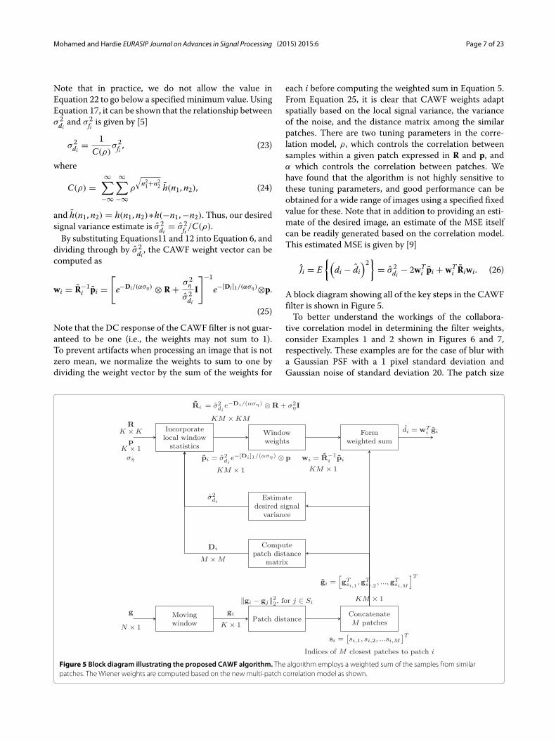
A block diagram showing all of the key steps in the CAWFfilter is shown in Figure 5.To better understand the workings of the collabora-

tive correlation model in determining the filter weights,consider Examples 1 and 2 shown in Figures 6 and 7,respectively. These examples are for the case of blur witha Gaussian PSF with a 1 pixel standard deviation andGaussian noise of standard deviation 20. The patch size

Figure 5 Block diagram illustrating the proposed CAWF algorithm. The algorithm employs a weighted sum of the samples from similarpatches. The Wiener weights are computed based on the new multi-patch correlation model as shown.


Patch 1 (Reference) Patch 2 Patch 3 Patch 4

(a)

Weights 1 Weights 2 Weights 3 Weights 4

(b)

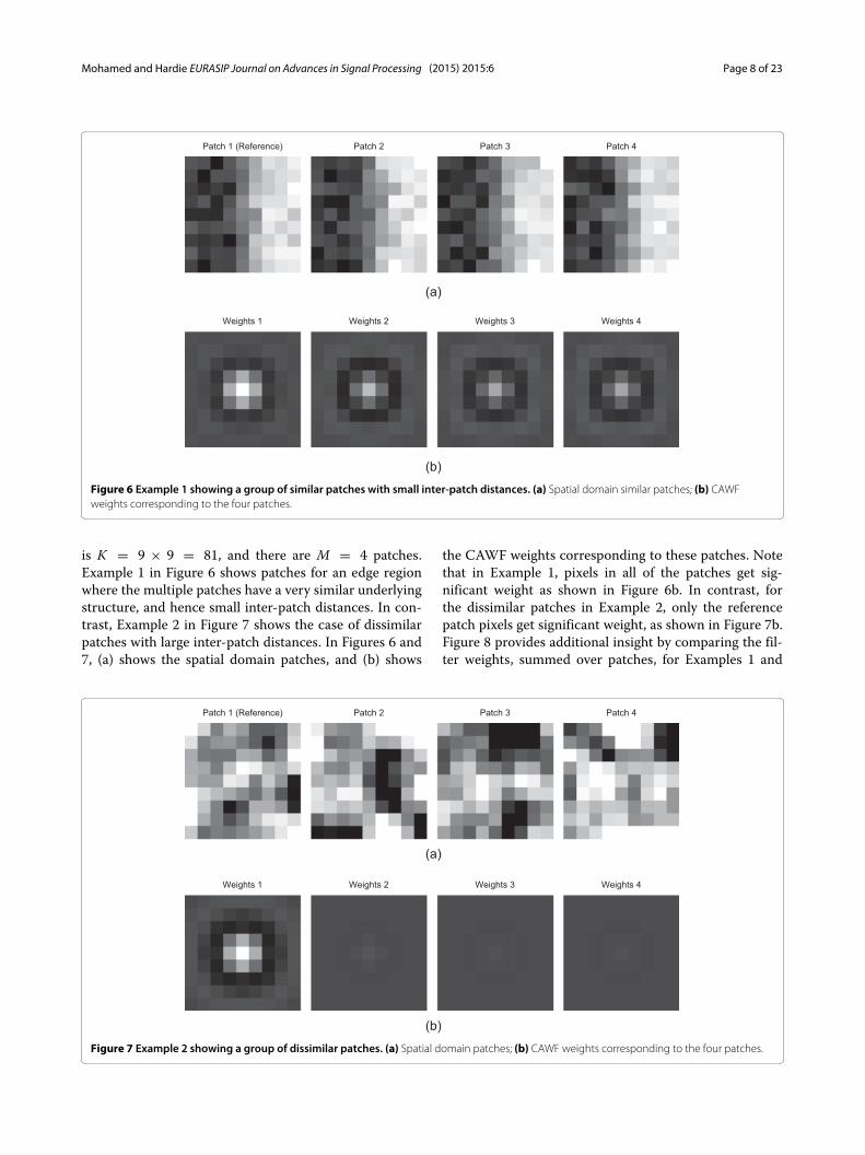
Figure 6 Example 1 showing a group of similar patches with small inter-patch distances. (a) Spatial domain similar patches; (b) CAWFweights corresponding to the four patches.

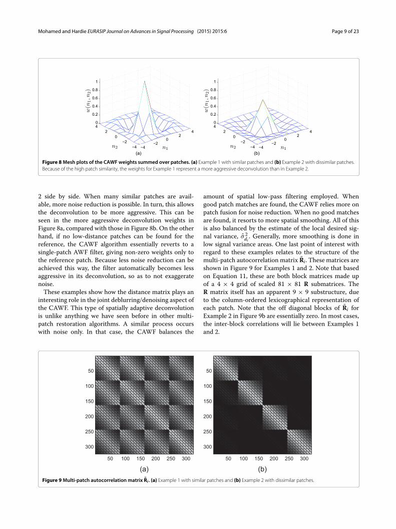
is K = 9 × 9 = 81, and there are M = 4 patches.Example 1 in Figure 6 shows patches for an edge regionwhere the multiple patches have a very similar underlyingstructure, and hence small inter-patch distances. In con-trast, Example 2 in Figure 7 shows the case of dissimilarpatches with large inter-patch distances. In Figures 6 and7, (a) shows the spatial domain patches, and (b) shows

the CAWF weights corresponding to these patches. Notethat in Example 1, pixels in all of the patches get sig-nificant weight as shown in Figure 6b. In contrast, forthe dissimilar patches in Example 2, only the referencepatch pixels get significant weight, as shown in Figure 7b.Figure 8 provides additional insight by comparing the fil-ter weights, summed over patches, for Examples 1 and

Patch 1 (Reference) Patch 2 Patch 3 Patch 4

(a)

Weights 1 Weights 2 Weights 3 Weights 4

(b)

Figure 7 Example 2 showing a group of dissimilar patches. (a) Spatial domain patches; (b) CAWF weights corresponding to the four patches.


Figure 8Mesh plots of the CAWF weights summed over patches. (a) Example 1 with similar patches and (b) Example 2 with dissimilar patches.Because of the high patch similarity, the weights for Example 1 represent a more aggressive deconvolution than in Example 2.

2 side by side. When many similar patches are avail-able, more noise reduction is possible. In turn, this allowsthe deconvolution to be more aggressive. This can beseen in the more aggressive deconvolution weights inFigure 8a, compared with those in Figure 8b. On the otherhand, if no low-distance patches can be found for thereference, the CAWF algorithm essentially reverts to asingle-patch AWF filter, giving non-zero weights only tothe reference patch. Because less noise reduction can beachieved this way, the filter automatically becomes lessaggressive in its deconvolution, so as to not exaggeratenoise.These examples show how the distance matrix plays an

interesting role in the joint deblurring/denoising aspect ofthe CAWF. This type of spatially adaptive deconvolutionis unlike anything we have seen before in other multi-patch restoration algorithms. A similar process occurswith noise only. In that case, the CAWF balances the

amount of spatial low-pass filtering employed. Whengood patch matches are found, the CAWF relies more onpatch fusion for noise reduction. When no good matchesare found, it resorts to more spatial smoothing. All of thisis also balanced by the estimate of the local desired sig-nal variance, σ 2

di . Generally, more smoothing is done inlow signal variance areas. One last point of interest withregard to these examples relates to the structure of themulti-patch autocorrelation matrix Ri. These matrices areshown in Figure 9 for Examples 1 and 2. Note that basedon Equation 11, these are both block matrices made upof a 4 × 4 grid of scaled 81 × 81 R submatrices. TheR matrix itself has an apparent 9 × 9 substructure, dueto the column-ordered lexicographical representation ofeach patch. Note that the off diagonal blocks of Ri forExample 2 in Figure 9b are essentially zero. In most cases,the inter-block correlations will lie between Examples 1and 2.

(a)50 100 150 200 250 300

50

100

150

200

250

300

(b)50 100 150 200 250 300

50

100

150

200

250

300

Figure 9Multi-patch autocorrelation matrix Ri . (a) Example 1 with similar patches and (b) Example 2 with dissimilar patches.


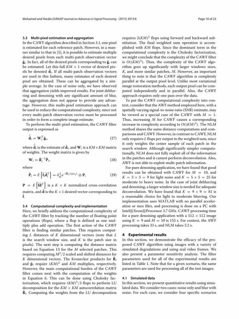
3.3 Multi-pixel estimation and aggregationIn the CAWF algorithm described in Section 3.1, one pixelis estimated for each reference patch. However, in a man-ner similar to that in [5], it is possible to estimate multipledesired pixels from each multi-patch observation vectorgi. In fact, all of the desired pixels corresponding to gi canbe estimated. Let this full KM × 1 vector of desired pix-els be denoted di. If all multi-patch observation vectorsare used in this fashion, many estimates of each desiredpixel are obtained. These can be aggregated by a sim-ple average. In the case of noise only, we have observedthat aggregation yields improved results. For joint deblur-ring and denoising with any significant amount of blur,the aggregation does not appear to provide any advan-tage. However, this multi-pixel estimation approach canbe used to reduce the computational complexity, since notevery multi-patch observation vector must be processedin order to form a complete image estimate.To perform the multi-pixel estimation, the CAWF filter

output is expressed as

ˆdi = WTi gi, (27)

where ˆdi is the estimate of di, andWi is aKM×KMmatrixof weights. The weight matrix is given by

Wi = R−1i Pi, (28)

where

Pi = E{fidTi

}= σ 2

die−Di/(αση) ⊗ P, (29)

P = E{fdT}is a K × K normalized cross-correlation

matrix, and d is the K ×1 desired vector corresponding tof.

3.4 Computational complexity and implementationHere, we briefly address the computational complexity ofthe CAWF filter by tracking the number of floating pointoperations (flops), where a flop is defined as one mul-tiply plus add operation. The first action of the CAWFfilter is finding similar patches. This requires comput-ing L distances of K dimensional vectors (note that Lis the search window size, and K is the patch size inpixels). The next step is computing the distance matrixbased on Equation 13 for the M selected patches. Thisrequires computingM2/2 scaled and shifted distances forK dimensional vectors. The Kronecker products for Riand pi require (KM)2 and KM multiplies, respectively.However, the main computational burden of the CAWFfilter comes next with the computation of the weightsin Equation 6. This can be done using Cholesky fac-torization, which requires (KM)3/3 flops to perform LUdecomposition for the KM × KM autocorrelation matrixRi. Computing the weights from the LU decomposition

requires 2(KM)2 flops using forward and backward sub-stitution. The final weighted sum operation is accom-plished with KM flops. Since the dominant term in thecomputational complexity is the Cholesky factorization,we might conclude that the complexity of the CAWF filteris O((KM)3). Thus, the complexity of the CAWF algo-rithm goes up significantly with larger windows sizes,K, and more similar patches, M. However, an importantthing to note is that the CAWF algorithm is completelyparallel at the output pixel level. Unlike most variationalimage restoration methods, each output pixel can be com-puted independently and in parallel. Also, the CAWFapproach requires only one pass over the data.To put the CAWF computational complexity into con-

text, consider that the AWFmethod employed here, with aspatially varying signal-to-noise ratio (SNR) estimate, maybe viewed as a special case of the CAWF with M = 1.Thus, increasing M for CAWF causes a correspondingincrease in complexity according to O((KM)3). The NLMmethod shares the same distance computations and com-parisons and CAWF. However, in contrast to CAWF, NLMonly requires L flops per output in the weighted sum, sinceit only weights the center sample of each patch in thesearch window. Although significantly simpler computa-tionally, NLM does not fully exploit all of the informationin the patches and it cannot perform deconvolution. Also,AWF is not able to exploit multi-patch information.For pure denoising application, we have found that good

results can be obtained with CAWF for M = 10, andK = 3 × 3 = 9 for light noise and K = 5 × 5 = 25 formoderate to heavy noise. In the case of joint deblurringand denoising, a larger window size is needed for adequatedeconvolution. We have found that K = 9 × 9 = 81 isa reasonable choice for light to moderate blurring. Ourimplementation uses MATLAB with no parallel acceler-ation or mex files, and processing is done on a PC withIntel�Xeon�Processor 3.7 GHz. CAWF processing timefor a pure denoising application with a 512 × 512 imageusing K = 9 and M = 10 is 155 s. For context, the AWFprocessing takes 33 s, and NLM takes 3.2 s.

4 Experimental resultsIn this section, we demonstrate the efficacy of the pro-posed CAWF algorithm using images with a variety ofsimulated degradations and using real video frames. Wealso present a parameter sensitivity analysis. The filterparameters used for all of the experimental results arelisted in Table 1. Note that for a given scenario, the sameparameters are used for processing all of the test images.

4.1 Simulated dataIn this section, we present quantitative results using simu-lated data.We consider two cases: noise only and blur withnoise. For each case, we consider four specific scenarios


Table 1 CAWF parameters used in experimental results

Case 1: noise only Case 2: blur and noise

Parameter name Variable Selected value Selected value Selected value

ση < 20 ση ≥ 20

Patch size K 3 × 3 = 9 5 × 5 = 25 9 × 9 = 81

Search window size L 17 × 17 = 289 11 × 11 = 121 9 × 9 = 81

Number of patches M 10 10 8

Autocorrelation decay ρ 0.65 0.70 0.65

Patch similarity decay α 2.00 1.40 1.20

Distance offset D0 0.25 0.50 0.00

Aggregation N/A Averaging Averaging None

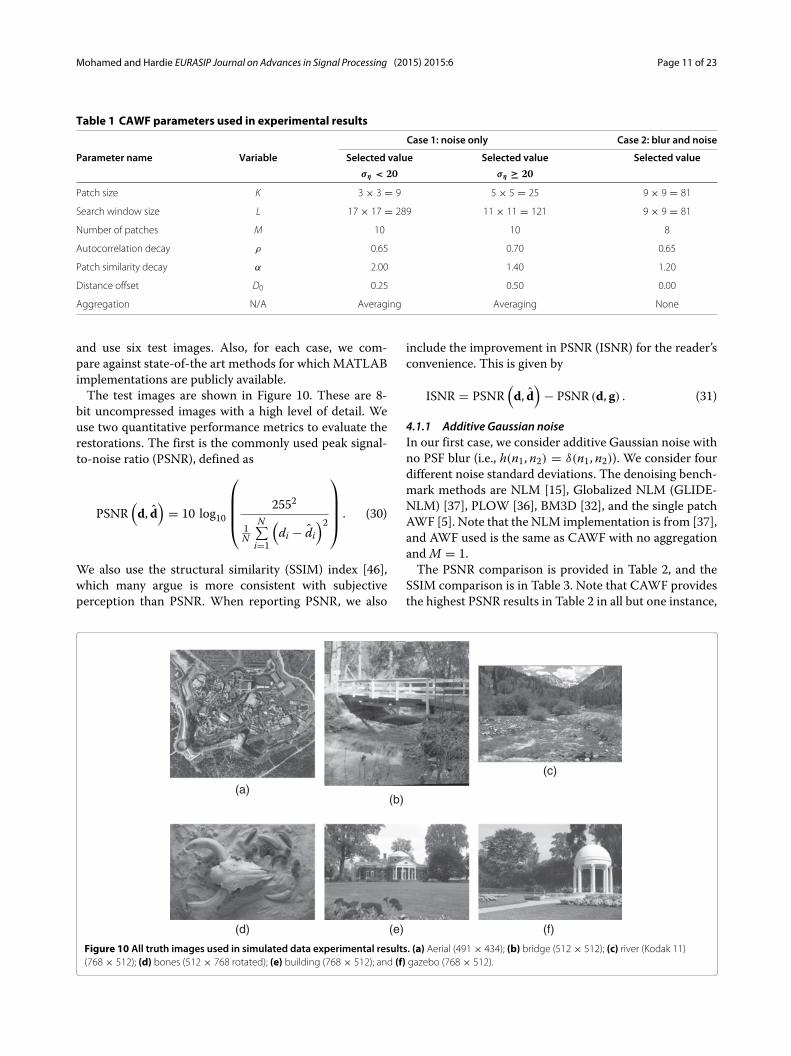
and use six test images. Also, for each case, we com-pare against state-of-the art methods for which MATLABimplementations are publicly available.The test images are shown in Figure 10. These are 8-

bit uncompressed images with a high level of detail. Weuse two quantitative performance metrics to evaluate therestorations. The first is the commonly used peak signal-to-noise ratio (PSNR), defined as

PSNR(d, d)

= 10 log10

⎛⎜⎜⎜⎝ 2552

1N

N∑i=1

(di − di

)2⎞⎟⎟⎟⎠ . (30)

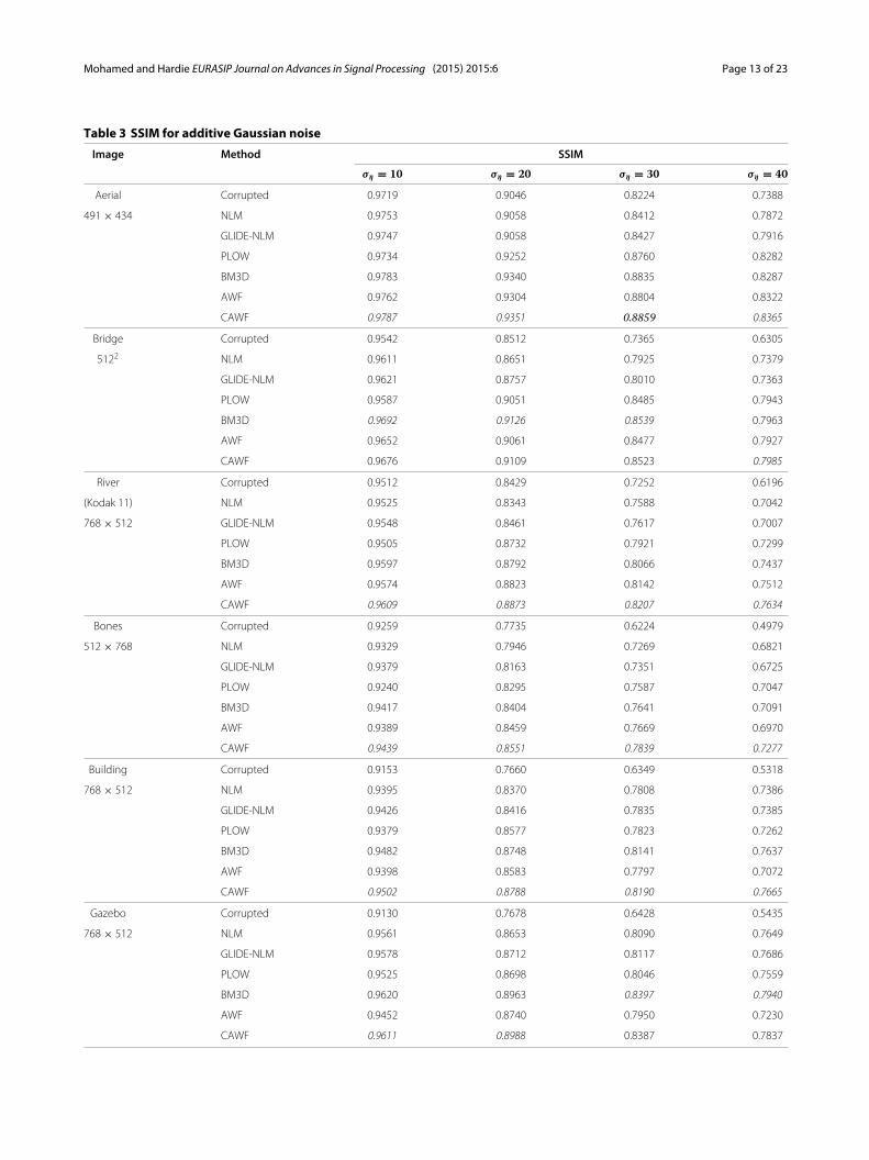
We also use the structural similarity (SSIM) index [46],which many argue is more consistent with subjectiveperception than PSNR. When reporting PSNR, we also

include the improvement in PSNR (ISNR) for the reader’sconvenience. This is given by

ISNR = PSNR(d, d)

− PSNR (d, g) . (31)

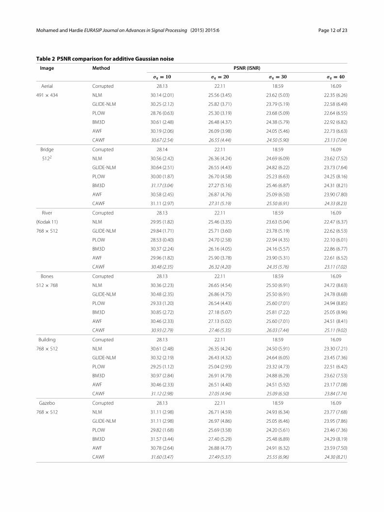
4.1.1 Additive Gaussian noiseIn our first case, we consider additive Gaussian noise withno PSF blur (i.e., h(n1, n2) = δ(n1, n2)). We consider fourdifferent noise standard deviations. The denoising bench-mark methods are NLM [15], Globalized NLM (GLIDE-NLM) [37], PLOW [36], BM3D [32], and the single patchAWF [5]. Note that the NLM implementation is from [37],and AWF used is the same as CAWF with no aggregationandM = 1.The PSNR comparison is provided in Table 2, and the

SSIM comparison is in Table 3. Note that CAWF providesthe highest PSNR results in Table 2 in all but one instance,

(a)(b)

(c)

(d) (e) (f)

Figure 10 All truth images used in simulated data experimental results. (a) Aerial (491 × 434); (b) bridge (512 × 512); (c) river (Kodak 11)(768 × 512); (d) bones (512 × 768 rotated); (e) building (768 × 512); and (f) gazebo (768 × 512).


Table 2 PSNR comparison for additive Gaussian noise

Image Method PSNR (ISNR)

ση = 10 ση = 20 ση = 30 ση = 40

Aerial Corrupted 28.13 22.11 18.59 16.09

491 × 434 NLM 30.14 (2.01) 25.56 (3.45) 23.62 (5.03) 22.35 (6.26)

GLIDE-NLM 30.25 (2.12) 25.82 (3.71) 23.79 (5.19) 22.58 (6.49)

PLOW 28.76 (0.63) 25.30 (3.19) 23.68 (5.09) 22.64 (6.55)

BM3D 30.61 (2.48) 26.48 (4.37) 24.38 (5.79) 22.92 (6.82)

AWF 30.19 (2.06) 26.09 (3.98) 24.05 (5.46) 22.73 (6.63)

CAWF 30.67 (2.54) 26.55 (4.44) 24.50 (5.90) 23.13 (7.04)

Bridge Corrupted 28.14 22.11 18.59 16.09

5122 NLM 30.56 (2.42) 26.36 (4.24) 24.69 (6.09) 23.62 (7.52)

GLIDE-NLM 30.64 (2.51) 26.55 (4.43) 24.82 (6.22) 23.73 (7.64)

PLOW 30.00 (1.87) 26.70 (4.58) 25.23 (6.63) 24.25 (8.16)

BM3D 31.17 (3.04) 27.27 (5.16) 25.46 (6.87) 24.31 (8.21)

AWF 30.58 (2.45) 26.87 (4.76) 25.09 (6.50) 23.90 (7.80)

CAWF 31.11 (2.97) 27.31 (5.19) 25.50 (6.91) 24.33 (8.23)

River Corrupted 28.13 22.11 18.59 16.09

(Kodak 11) NLM 29.95 (1.82) 25.46 (3.35) 23.63 (5.04) 22.47 (6.37)

768 × 512 GLIDE-NLM 29.84 (1.71) 25.71 (3.60) 23.78 (5.19) 22.62 (6.53)

PLOW 28.53 (0.40) 24.70 (2.58) 22.94 (4.35) 22.10 (6.01)

BM3D 30.37 (2.24) 26.16 (4.05) 24.16 (5.57) 22.86 (6.77)

AWF 29.96 (1.82) 25.90 (3.78) 23.90 (5.31) 22.61 (6.52)

CAWF 30.48 (2.35) 26.32 (4.20) 24.35 (5.76) 23.11 (7.02)

Bones Corrupted 28.13 22.11 18.59 16.09

512 × 768 NLM 30.36 (2.23) 26.65 (4.54) 25.50 (6.91) 24.72 (8.63)

GLIDE-NLM 30.48 (2.35) 26.86 (4.75) 25.50 (6.91) 24.78 (8.68)

PLOW 29.33 (1.20) 26.54 (4.43) 25.60 (7.01) 24.94 (8.85)

BM3D 30.85 (2.72) 27.18 (5.07) 25.81 (7.22) 25.05 (8.96)

AWF 30.46 (2.33) 27.13 (5.02) 25.60 (7.01) 24.51 (8.41)

CAWF 30.93 (2.79) 27.46 (5.35) 26.03 (7.44) 25.11 (9.02)

Building Corrupted 28.13 22.11 18.59 16.09

768 × 512 NLM 30.61 (2.48) 26.35 (4.24) 24.50 (5.91) 23.30 (7.21)

GLIDE-NLM 30.32 (2.19) 26.43 (4.32) 24.64 (6.05) 23.45 (7.36)

PLOW 29.25 (1.12) 25.04 (2.93) 23.32 (4.73) 22.51 (6.42)

BM3D 30.97 (2.84) 26.91 (4.79) 24.88 (6.29) 23.62 (7.53)

AWF 30.46 (2.33) 26.51 (4.40) 24.51 (5.92) 23.17 (7.08)

CAWF 31.12 (2.98) 27.05 (4.94) 25.09 (6.50) 23.84 (7.74)

Gazebo Corrupted 28.13 22.11 18.59 16.09

768 × 512 NLM 31.11 (2.98) 26.71 (4.59) 24.93 (6.34) 23.77 (7.68)

GLIDE-NLM 31.11 (2.98) 26.97 (4.86) 25.05 (6.46) 23.95 (7.86)

PLOW 29.82 (1.68) 25.69 (3.58) 24.20 (5.61) 23.46 (7.36)

BM3D 31.57 (3.44) 27.40 (5.29) 25.48 (6.89) 24.29 (8.19)

AWF 30.78 (2.64) 26.88 (4.77) 24.91 (6.32) 23.59 (7.50)

CAWF 31.60 (3.47) 27.49 (5.37) 25.55 (6.96) 24.30 (8.21)


Table 3 SSIM for additive Gaussian noise

Image Method SSIM

ση = 10 ση = 20 ση = 30 ση = 40


491 × 434 NLM 0.9753 0.9058 0.8412 0.7872

GLIDE-NLM 0.9747 0.9058 0.8427 0.7916

PLOW 0.9734 0.9252 0.8760 0.8282

BM3D 0.9783 0.9340 0.8835 0.8287

AWF 0.9762 0.9304 0.8804 0.8322

CAWF 0.9787 0.9351 0.8859 0.8365


5122 NLM 0.9611 0.8651 0.7925 0.7379

GLIDE-NLM 0.9621 0.8757 0.8010 0.7363

PLOW 0.9587 0.9051 0.8485 0.7943

BM3D 0.9692 0.9126 0.8539 0.7963

AWF 0.9652 0.9061 0.8477 0.7927

CAWF 0.9676 0.9109 0.8523 0.7985

River Corrupted 0.9512 0.8429 0.7252 0.6196

(Kodak 11) NLM 0.9525 0.8343 0.7588 0.7042

768 × 512 GLIDE-NLM 0.9548 0.8461 0.7617 0.7007

PLOW 0.9505 0.8732 0.7921 0.7299

BM3D 0.9597 0.8792 0.8066 0.7437

AWF 0.9574 0.8823 0.8142 0.7512

CAWF 0.9609 0.8873 0.8207 0.7634

Bones Corrupted 0.9259 0.7735 0.6224 0.4979

512 × 768 NLM 0.9329 0.7946 0.7269 0.6821

GLIDE-NLM 0.9379 0.8163 0.7351 0.6725

PLOW 0.9240 0.8295 0.7587 0.7047

BM3D 0.9417 0.8404 0.7641 0.7091

AWF 0.9389 0.8459 0.7669 0.6970

CAWF 0.9439 0.8551 0.7839 0.7277


768 × 512 NLM 0.9395 0.8370 0.7808 0.7386

GLIDE-NLM 0.9426 0.8416 0.7835 0.7385

PLOW 0.9379 0.8577 0.7823 0.7262

BM3D 0.9482 0.8748 0.8141 0.7637

AWF 0.9398 0.8583 0.7797 0.7072

CAWF 0.9502 0.8788 0.8190 0.7665


768 × 512 NLM 0.9561 0.8653 0.8090 0.7649

GLIDE-NLM 0.9578 0.8712 0.8117 0.7686

PLOW 0.9525 0.8698 0.8046 0.7559

BM3D 0.9620 0.8963 0.8397 0.7940

AWF 0.9452 0.8740 0.7950 0.7230

CAWF 0.9611 0.8988 0.8387 0.7837


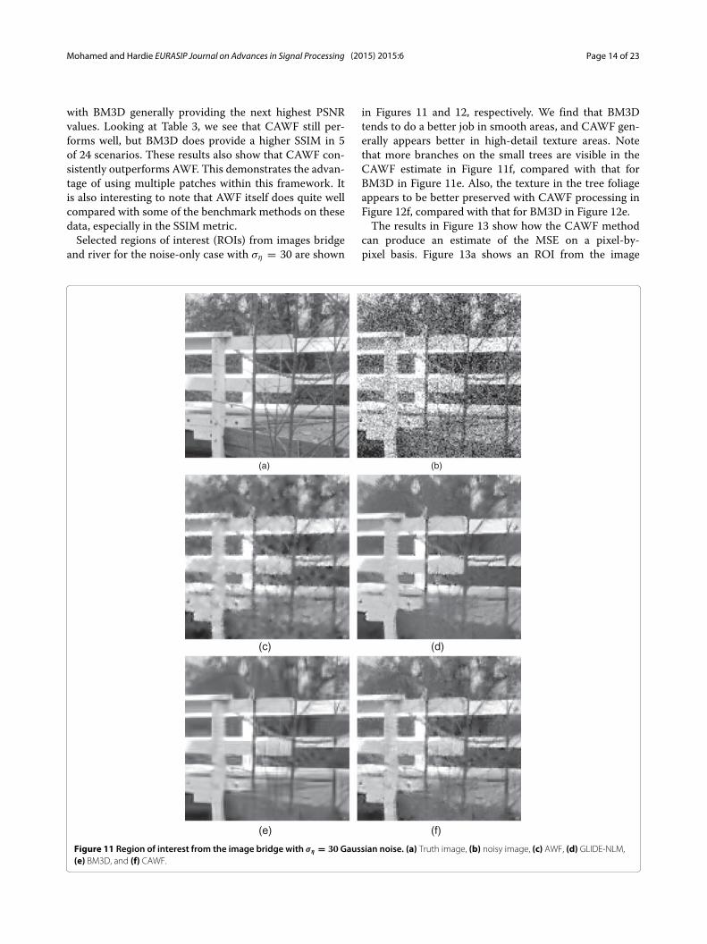
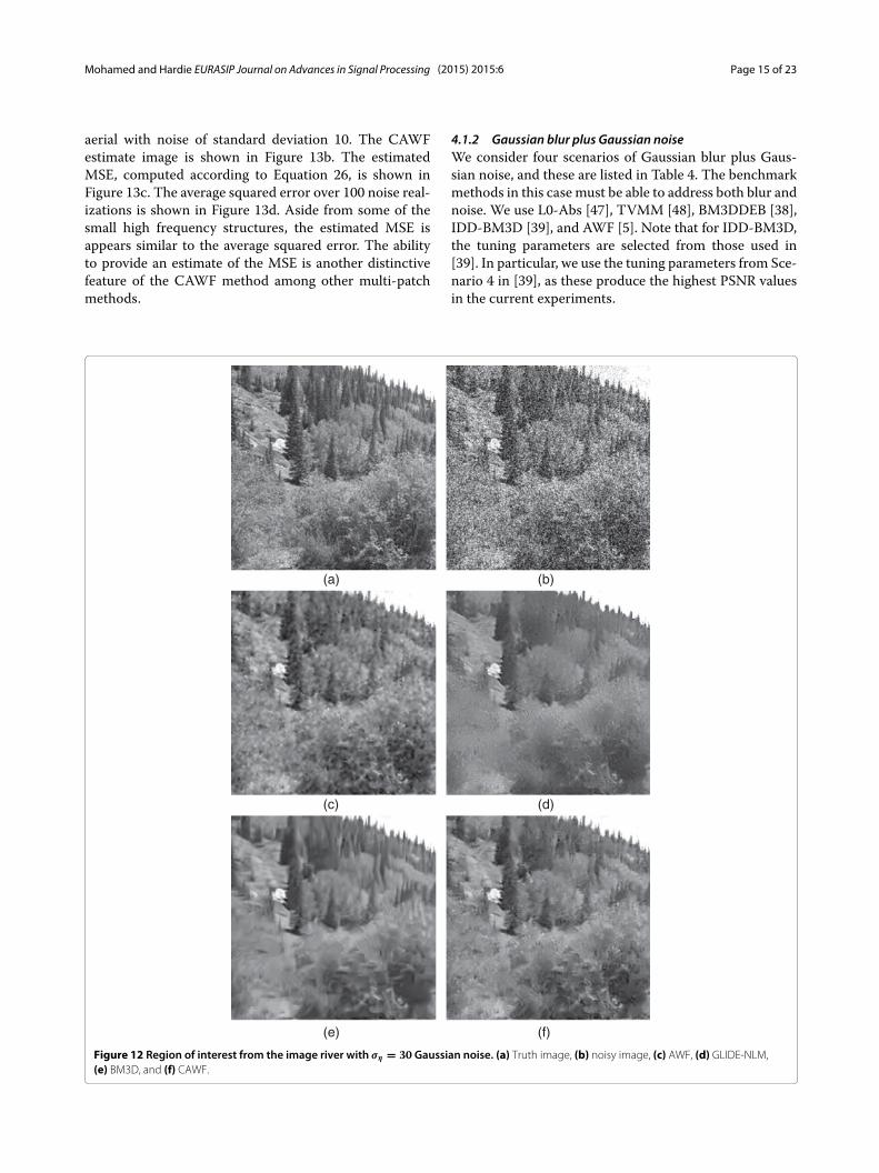
with BM3D generally providing the next highest PSNRvalues. Looking at Table 3, we see that CAWF still per-forms well, but BM3D does provide a higher SSIM in 5of 24 scenarios. These results also show that CAWF con-sistently outperforms AWF. This demonstrates the advan-tage of using multiple patches within this framework. Itis also interesting to note that AWF itself does quite wellcompared with some of the benchmark methods on thesedata, especially in the SSIM metric.Selected regions of interest (ROIs) from images bridge

and river for the noise-only case with ση = 30 are shown

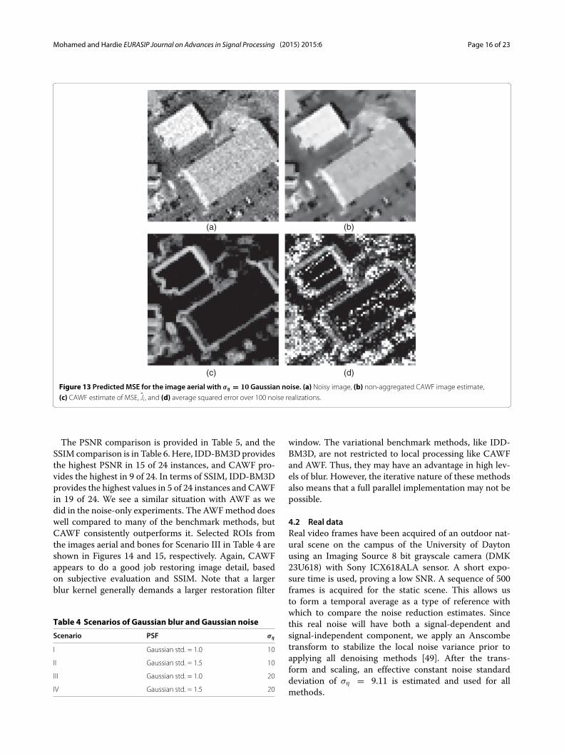
in Figures 11 and 12, respectively. We find that BM3Dtends to do a better job in smooth areas, and CAWF gen-erally appears better in high-detail texture areas. Notethat more branches on the small trees are visible in theCAWF estimate in Figure 11f, compared with that forBM3D in Figure 11e. Also, the texture in the tree foliageappears to be better preserved with CAWF processing inFigure 12f, compared with that for BM3D in Figure 12e.The results in Figure 13 show how the CAWF method

can produce an estimate of the MSE on a pixel-by-pixel basis. Figure 13a shows an ROI from the image

(a) (b)

(c) (d)

(e) (f)

Figure 11 Region of interest from the image bridge with ση = 30 Gaussian noise. (a) Truth image, (b) noisy image, (c) AWF, (d) GLIDE-NLM,(e) BM3D, and (f) CAWF.


aerial with noise of standard deviation 10. The CAWFestimate image is shown in Figure 13b. The estimatedMSE, computed according to Equation 26, is shown inFigure 13c. The average squared error over 100 noise real-izations is shown in Figure 13d. Aside from some of thesmall high frequency structures, the estimated MSE isappears similar to the average squared error. The abilityto provide an estimate of the MSE is another distinctivefeature of the CAWF method among other multi-patchmethods.

4.1.2 Gaussian blur plus Gaussian noiseWe consider four scenarios of Gaussian blur plus Gaus-sian noise, and these are listed in Table 4. The benchmarkmethods in this case must be able to address both blur andnoise. We use L0-Abs [47], TVMM [48], BM3DDEB [38],IDD-BM3D [39], and AWF [5]. Note that for IDD-BM3D,the tuning parameters are selected from those used in[39]. In particular, we use the tuning parameters from Sce-nario 4 in [39], as these produce the highest PSNR valuesin the current experiments.

(a) (b)

(c) (d)

(e) (f)

Figure 12 Region of interest from the image river with ση = 30 Gaussian noise. (a) Truth image, (b) noisy image, (c) AWF, (d) GLIDE-NLM,(e) BM3D, and (f) CAWF.


(a) (b)

(c) (d)

Figure 13 Predicted MSE for the image aerial with ση = 10 Gaussian noise. (a) Noisy image, (b) non-aggregated CAWF image estimate,

(c) CAWF estimate of MSE, Ji , and (d) average squared error over 100 noise realizations.

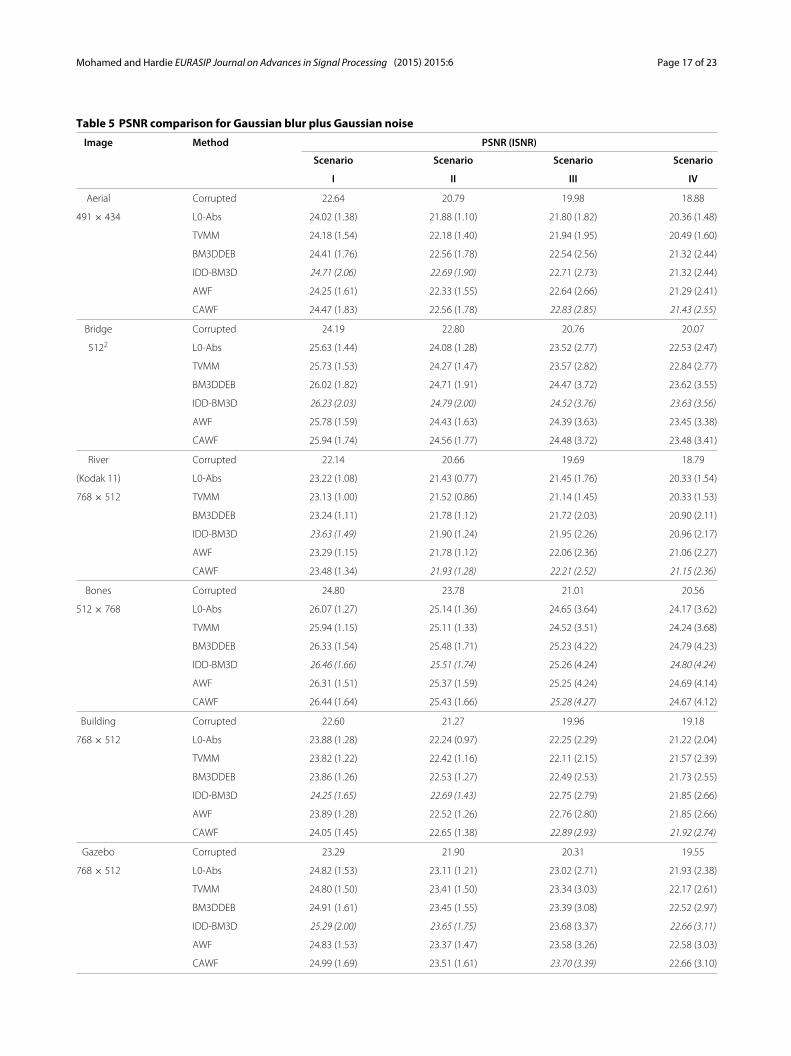
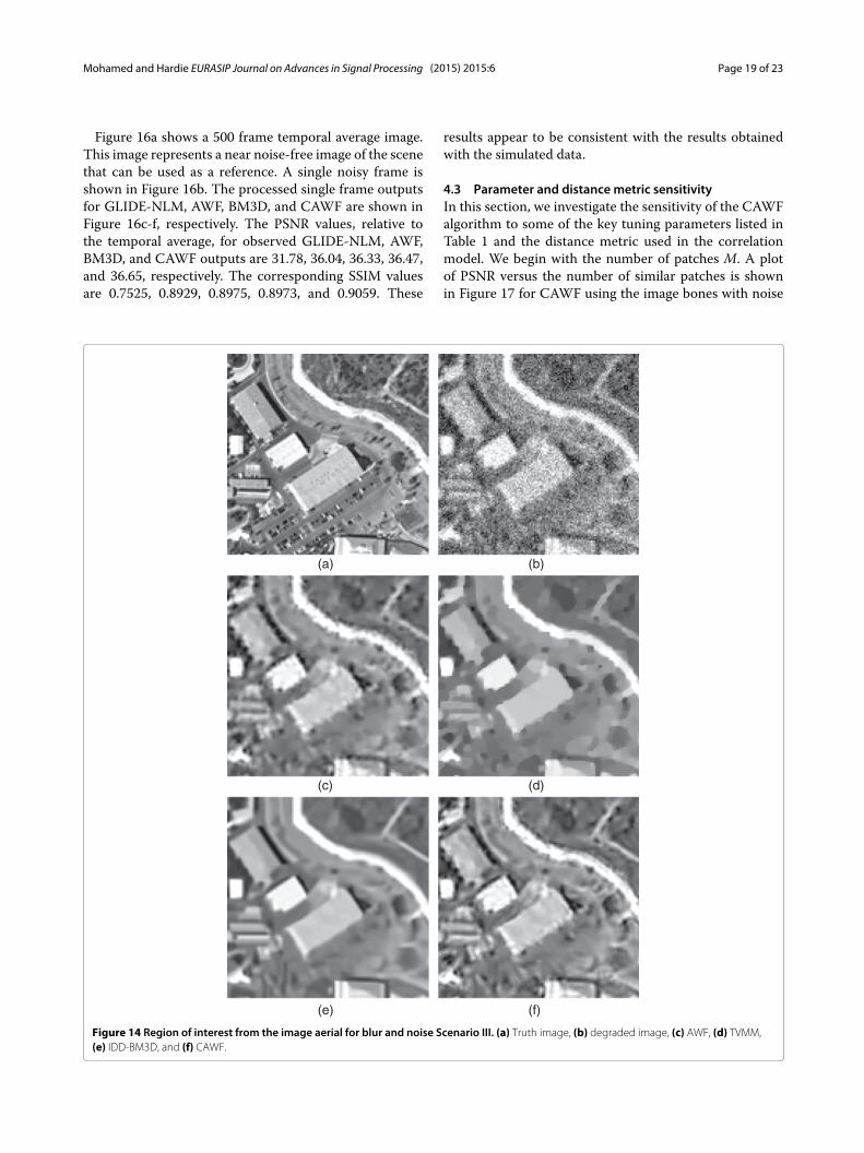
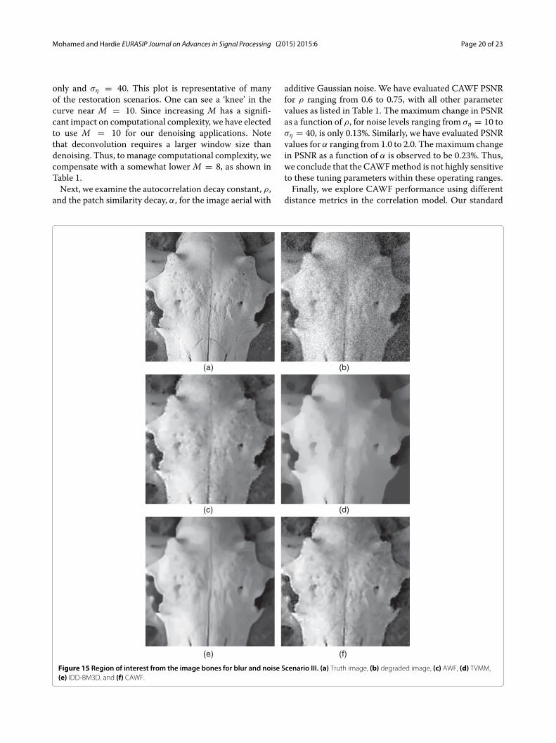
The PSNR comparison is provided in Table 5, and theSSIM comparison is in Table 6. Here, IDD-BM3Dprovidesthe highest PSNR in 15 of 24 instances, and CAWF pro-vides the highest in 9 of 24. In terms of SSIM, IDD-BM3Dprovides the highest values in 5 of 24 instances and CAWFin 19 of 24. We see a similar situation with AWF as wedid in the noise-only experiments. The AWFmethod doeswell compared to many of the benchmark methods, butCAWF consistently outperforms it. Selected ROIs fromthe images aerial and bones for Scenario III in Table 4 areshown in Figures 14 and 15, respectively. Again, CAWFappears to do a good job restoring image detail, basedon subjective evaluation and SSIM. Note that a largerblur kernel generally demands a larger restoration filter

Table 4 Scenarios of Gaussian blur and Gaussian noise

Scenario PSF ση

I Gaussian std. = 1.0 10

II Gaussian std. = 1.5 10

III Gaussian std. = 1.0 20

IV Gaussian std. = 1.5 20

window. The variational benchmark methods, like IDD-BM3D, are not restricted to local processing like CAWFand AWF. Thus, they may have an advantage in high lev-els of blur. However, the iterative nature of these methodsalso means that a full parallel implementation may not bepossible.

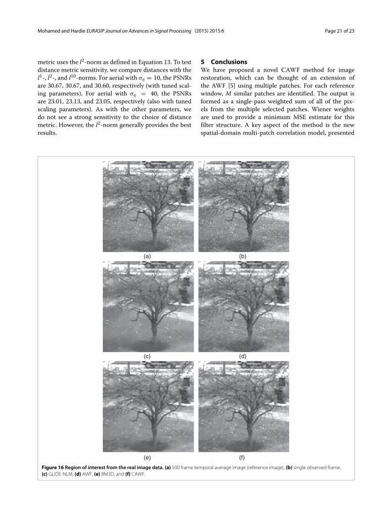
4.2 Real dataReal video frames have been acquired of an outdoor nat-ural scene on the campus of the University of Daytonusing an Imaging Source 8 bit grayscale camera (DMK23U618) with Sony ICX618ALA sensor. A short expo-sure time is used, proving a low SNR. A sequence of 500frames is acquired for the static scene. This allows usto form a temporal average as a type of reference withwhich to compare the noise reduction estimates. Sincethis real noise will have both a signal-dependent andsignal-independent component, we apply an Anscombetransform to stabilize the local noise variance prior toapplying all denoising methods [49]. After the trans-form and scaling, an effective constant noise standarddeviation of ση = 9.11 is estimated and used for allmethods.


Table 5 PSNR comparison for Gaussian blur plus Gaussian noise

Image Method PSNR (ISNR)

Scenario Scenario Scenario Scenario

I II III IV


491 × 434 L0-Abs 24.02 (1.38) 21.88 (1.10) 21.80 (1.82) 20.36 (1.48)

TVMM 24.18 (1.54) 22.18 (1.40) 21.94 (1.95) 20.49 (1.60)

BM3DDEB 24.41 (1.76) 22.56 (1.78) 22.54 (2.56) 21.32 (2.44)

IDD-BM3D 24.71 (2.06) 22.69 (1.90) 22.71 (2.73) 21.32 (2.44)

AWF 24.25 (1.61) 22.33 (1.55) 22.64 (2.66) 21.29 (2.41)

CAWF 24.47 (1.83) 22.56 (1.78) 22.83 (2.85) 21.43 (2.55)


5122 L0-Abs 25.63 (1.44) 24.08 (1.28) 23.52 (2.77) 22.53 (2.47)

TVMM 25.73 (1.53) 24.27 (1.47) 23.57 (2.82) 22.84 (2.77)

BM3DDEB 26.02 (1.82) 24.71 (1.91) 24.47 (3.72) 23.62 (3.55)

IDD-BM3D 26.23 (2.03) 24.79 (2.00) 24.52 (3.76) 23.63 (3.56)

AWF 25.78 (1.59) 24.43 (1.63) 24.39 (3.63) 23.45 (3.38)

CAWF 25.94 (1.74) 24.56 (1.77) 24.48 (3.72) 23.48 (3.41)

River Corrupted 22.14 20.66 19.69 18.79

(Kodak 11) L0-Abs 23.22 (1.08) 21.43 (0.77) 21.45 (1.76) 20.33 (1.54)

768 × 512 TVMM 23.13 (1.00) 21.52 (0.86) 21.14 (1.45) 20.33 (1.53)

BM3DDEB 23.24 (1.11) 21.78 (1.12) 21.72 (2.03) 20.90 (2.11)

IDD-BM3D 23.63 (1.49) 21.90 (1.24) 21.95 (2.26) 20.96 (2.17)

AWF 23.29 (1.15) 21.78 (1.12) 22.06 (2.36) 21.06 (2.27)

CAWF 23.48 (1.34) 21.93 (1.28) 22.21 (2.52) 21.15 (2.36)

Bones Corrupted 24.80 23.78 21.01 20.56

512 × 768 L0-Abs 26.07 (1.27) 25.14 (1.36) 24.65 (3.64) 24.17 (3.62)

TVMM 25.94 (1.15) 25.11 (1.33) 24.52 (3.51) 24.24 (3.68)

BM3DDEB 26.33 (1.54) 25.48 (1.71) 25.23 (4.22) 24.79 (4.23)

IDD-BM3D 26.46 (1.66) 25.51 (1.74) 25.26 (4.24) 24.80 (4.24)

AWF 26.31 (1.51) 25.37 (1.59) 25.25 (4.24) 24.69 (4.14)

CAWF 26.44 (1.64) 25.43 (1.66) 25.28 (4.27) 24.67 (4.12)


768 × 512 L0-Abs 23.88 (1.28) 22.24 (0.97) 22.25 (2.29) 21.22 (2.04)

TVMM 23.82 (1.22) 22.42 (1.16) 22.11 (2.15) 21.57 (2.39)

BM3DDEB 23.86 (1.26) 22.53 (1.27) 22.49 (2.53) 21.73 (2.55)

IDD-BM3D 24.25 (1.65) 22.69 (1.43) 22.75 (2.79) 21.85 (2.66)

AWF 23.89 (1.28) 22.52 (1.26) 22.76 (2.80) 21.85 (2.66)

CAWF 24.05 (1.45) 22.65 (1.38) 22.89 (2.93) 21.92 (2.74)


768 × 512 L0-Abs 24.82 (1.53) 23.11 (1.21) 23.02 (2.71) 21.93 (2.38)

TVMM 24.80 (1.50) 23.41 (1.50) 23.34 (3.03) 22.17 (2.61)

BM3DDEB 24.91 (1.61) 23.45 (1.55) 23.39 (3.08) 22.52 (2.97)

IDD-BM3D 25.29 (2.00) 23.65 (1.75) 23.68 (3.37) 22.66 (3.11)

AWF 24.83 (1.53) 23.37 (1.47) 23.58 (3.26) 22.58 (3.03)

CAWF 24.99 (1.69) 23.51 (1.61) 23.70 (3.39) 22.66 (3.10)


Table 6 SSIM comparison for Gaussian blur plus Gaussian noise

Image Method SSIM

Scenario Scenario Scenario Scenario

I II III IV


491 × 434 L0-Abs 0.9087 0.8050 0.7821 0.6448

TVMM 0.9215 0.8325 0.7885 0.6604

BM3DDEB 0.9198 0.8571 0.8400 0.7710

IDD-BM3D 0.9292 0.8591 0.8406 0.7577

AWF 0.9199 0.8519 0.8517 0.7733

CAWF 0.9273 0.8662 0.8649 0.7957


5122 L0-Abs 0.8902 0.8044 0.7425 0.6524

TVMM 0.8995 0.8156 0.7323 0.6689

BM3DDEB 0.9099 0.8579 0.8294 0.7796

IDD-BM3D 0.9173 0.8573 0.8252 0.7657

AWF 0.9080 0.8503 0.8344 0.7712

CAWF 0.9155 0.8637 0.8462 0.7892

River Corrupted 0.8373 0.7198 0.7246 0.6161

(Kodak 11) L0-Abs 0.8328 0.7159 0.6670 0.5560

768 × 512 TVMM 0.8452 0.7219 0.6344 0.5421

BM3DDEB 0.8487 0.7713 0.7377 0.6745

IDD-BM3D 0.8672 0.7767 0.7463 0.6666

AWF 0.8573 0.7736 0.7676 0.6878

CAWF 0.8707 0.7949 0.7837 0.7105

Bones Corrupted 0.8231 0.7323 0.6681 0.5884

512 × 768 L0-Abs 0.8051 0.7287 0.6652 0.6181

TVMM 0.7954 0.7192 0.6427 0.6172

BM3DDEB 0.8320 0.7768 0.7420 0.7064

IDD-BM3D 0.8421 0.7753 0.7389 0.6969

AWF 0.8358 0.7699 0.7526 0.7000

CAWF 0.8476 0.7866 0.7615 0.7108


768 × 512 L0-Abs 0.8356 0.7491 0.7142 0.6397

TVMM 0.8454 0.7592 0.6936 0.6615

BM3DDEB 0.8520 0.7913 0.7633 0.7138

IDD-BM3D 0.8662 0.7953 0.7715 0.7130

AWF 0.8509 0.7848 0.7721 0.7147

CAWF 0.8607 0.7974 0.7816 0.7268


768 × 512 L0-Abs 0.8651 0.7867 0.7527 0.6788

TVMM 0.8741 0.8057 0.7785 0.6826

BM3DDEB 0.8805 0.8249 0.8001 0.7500

IDD-BM3D 0.8898 0.8282 0.8064 0.7504

AWF 0.8796 0.8190 0.8035 0.7481

CAWF 0.8801 0.8238 0.8072 0.7561


Figure 16a shows a 500 frame temporal average image.This image represents a near noise-free image of the scenethat can be used as a reference. A single noisy frame isshown in Figure 16b. The processed single frame outputsfor GLIDE-NLM, AWF, BM3D, and CAWF are shown inFigure 16c-f, respectively. The PSNR values, relative tothe temporal average, for observed GLIDE-NLM, AWF,BM3D, and CAWF outputs are 31.78, 36.04, 36.33, 36.47,and 36.65, respectively. The corresponding SSIM valuesare 0.7525, 0.8929, 0.8975, 0.8973, and 0.9059. These

results appear to be consistent with the results obtainedwith the simulated data.

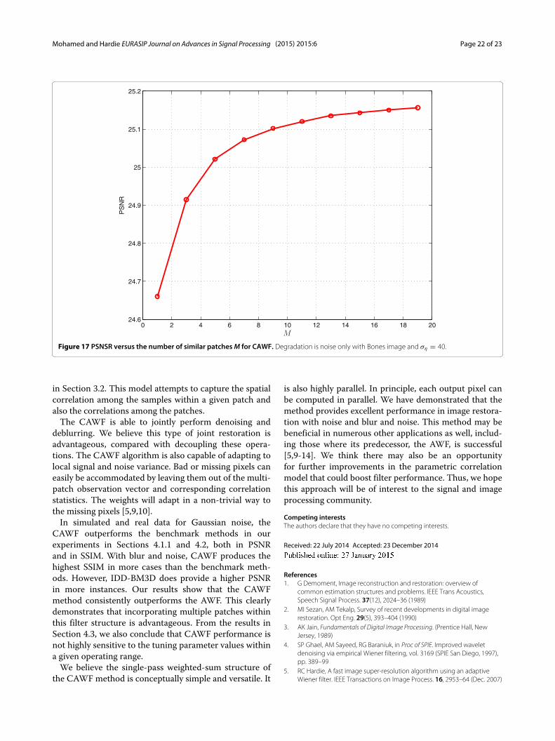
4.3 Parameter and distance metric sensitivityIn this section, we investigate the sensitivity of the CAWFalgorithm to some of the key tuning parameters listed inTable 1 and the distance metric used in the correlationmodel. We begin with the number of patches M. A plotof PSNR versus the number of similar patches is shownin Figure 17 for CAWF using the image bones with noise

(a) (b)

(c) (d)

(e) (f)

Figure 14 Region of interest from the image aerial for blur and noise Scenario III. (a) Truth image, (b) degraded image, (c) AWF, (d) TVMM,(e) IDD-BM3D, and (f) CAWF.


only and ση = 40. This plot is representative of manyof the restoration scenarios. One can see a ‘knee’ in thecurve near M = 10. Since increasing M has a signifi-cant impact on computational complexity, we have electedto use M = 10 for our denoising applications. Notethat deconvolution requires a larger window size thandenoising. Thus, to manage computational complexity, wecompensate with a somewhat lower M = 8, as shown inTable 1.Next, we examine the autocorrelation decay constant, ρ,

and the patch similarity decay, α, for the image aerial with

additive Gaussian noise. We have evaluated CAWF PSNRfor ρ ranging from 0.6 to 0.75, with all other parametervalues as listed in Table 1. The maximum change in PSNRas a function of ρ, for noise levels ranging from ση = 10 toση = 40, is only 0.13%. Similarly, we have evaluated PSNRvalues for α ranging from 1.0 to 2.0. Themaximum changein PSNR as a function of α is observed to be 0.23%. Thus,we conclude that the CAWFmethod is not highly sensitiveto these tuning parameters within these operating ranges.Finally, we explore CAWF performance using different

distance metrics in the correlation model. Our standard

(a) (b)

(c) (d)

(e) (f)

Figure 15 Region of interest from the image bones for blur and noise Scenario III. (a) Truth image, (b) degraded image, (c) AWF, (d) TVMM,(e) IDD-BM3D, and (f) CAWF.


metric uses the l2-norm as defined in Equation 13. To testdistance metric sensitivity, we compare distances with thel1-, l2-, and l10-norms. For aerial with ση = 10, the PSNRsare 30.67, 30.67, and 30.60, respectively (with tuned scal-ing parameters). For aerial with ση = 40, the PSNRsare 23.01, 23.13, and 23.05, respectively (also with tunedscaling parameters). As with the other parameters, wedo not see a strong sensitivity to the choice of distancemetric. However, the l2-norm generally provides the bestresults.

5 ConclusionsWe have proposed a novel CAWF method for imagerestoration, which can be thought of an extension ofthe AWF [5] using multiple patches. For each referencewindow, M similar patches are identified. The output isformed as a single-pass weighted sum of all of the pix-els from the multiple selected patches. Wiener weightsare used to provide a minimum MSE estimate for thisfilter structure. A key aspect of the method is the newspatial-domain multi-patch correlation model, presented

(a) (b)

(c) (d)

(e) (f)

Figure 16 Region of interest from the real image data. (a) 500 frame temporal average image (reference image), (b) single observed frame,(c) GLIDE-NLM, (d) AWF, (e) BM3D, and (f) CAWF.


0 2 4 6 8 10 12 14 16 18 2024.6

24.7

24.8

24.9

25

25.1

25.2

M

PSNR

Figure 17 PSNSR versus the number of similar patchesM for CAWF. Degradation is noise only with Bones image and ση = 40.

in Section 3.2. This model attempts to capture the spatialcorrelation among the samples within a given patch andalso the correlations among the patches.The CAWF is able to jointly perform denoising and

deblurring. We believe this type of joint restoration isadvantageous, compared with decoupling these opera-tions. The CAWF algorithm is also capable of adapting tolocal signal and noise variance. Bad or missing pixels caneasily be accommodated by leaving them out of the multi-patch observation vector and corresponding correlationstatistics. The weights will adapt in a non-trivial way tothe missing pixels [5,9,10].In simulated and real data for Gaussian noise, the

CAWF outperforms the benchmark methods in ourexperiments in Sections 4.1.1 and 4.2, both in PSNRand in SSIM. With blur and noise, CAWF produces thehighest SSIM in more cases than the benchmark meth-ods. However, IDD-BM3D does provide a higher PSNRin more instances. Our results show that the CAWFmethod consistently outperforms the AWF. This clearlydemonstrates that incorporating multiple patches withinthis filter structure is advantageous. From the results inSection 4.3, we also conclude that CAWF performance isnot highly sensitive to the tuning parameter values withina given operating range.We believe the single-pass weighted-sum structure of

the CAWF method is conceptually simple and versatile. It

is also highly parallel. In principle, each output pixel canbe computed in parallel. We have demonstrated that themethod provides excellent performance in image restora-tion with noise and blur and noise. This method may bebeneficial in numerous other applications as well, includ-ing those where its predecessor, the AWF, is successful[5,9-14]. We think there may also be an opportunityfor further improvements in the parametric correlationmodel that could boost filter performance. Thus, we hopethis approach will be of interest to the signal and imageprocessing community.

Competing interestsThe authors declare that they have no competing interests.

Received: 22 July 2014 Accepted: 23 December 2014

References1. G Demoment, Image reconstruction and restoration: overview of

common estimation structures and problems. IEEE Trans Acoustics,Speech Signal Process. 37(12), 2024–36 (1989)

2. MI Sezan, AM Tekalp, Survey of recent developments in digital imagerestoration. Opt Eng. 29(5), 393–404 (1990)

3. AK Jain, Fundamentals of Digital Image Processing. (Prentice Hall, NewJersey, 1989)

4. SP Ghael, AM Sayeed, RG Baraniuk, in Proc of SPIE. Improved waveletdenoising via empirical Wiener filtering, vol. 3169 (SPIE San Diego, 1997),pp. 389–99

5. RC Hardie, A fast image super-resolution algorithm using an adaptiveWiener filter. IEEE Transactions on Image Process. 16, 2953–64 (Dec. 2007)


6. KE Barner, AM Sarhan, RC Hardie, Partition-based weighted sum filters forimage restoration. IEEE Trans Image Process. 8, 740–745 (May 1999)

7. M Shao, KE Barner, RC Hardie, Partition-based interpolation for imagedemosaicing and super-resolution reconstruction. Opt Eng.44, 107003–1–107003–14 (Oct 2005)

8. B Narayanan, RC Hardie, KE Barner, M Shao, A computationally efficientsuper-resolution algorithm for video processing using partition filters.IEEE Trans Circuits Syst Video Technol. 17, 621–34 (May 2007)

9. RC Hardie, KJ Barnard, R Ordonez, Fast super-resolution with affinemotion using an adaptive Wiener filter and its application to airborneimaging. Opt Express, 1926208–31 (Dec 2011)

10. RC Hardie, KJ Barnard, Fast super-resolution using an adaptive Wiener filterwith robustness to local motion. Opt Express. 20, 21053–73 (Sep 2012)

11. B Narayanan, RC Hardie, E Balster, Multiframe adaptive Wiener filtersuper-resolution with JPEG2000-compressed images. EURASIP J AdvSignal Process. 2014(1), 55 (2014)

12. RC Hardie, DA LeMaster, BM Ratliff, Super-resolution for imagery fromintegrated microgrid polarimeters. Opt Express. 19, 12937–60 (Jul 2011)

13. BK Karch, RC Hardie, Adaptive Wiener filter super-resolution of color filterarray images. Opt Express, 2118820–41 (Aug 2013)

14. M Rucci, RC Hardie, KJ Barnard, 53. Appl Opt, C1–13 (May 2014)15. A Buades, B Coll, JM Morel, A review of image denoising algorithms, with

a new one. Multiscale Model Simul. 4, 490–530 (2005)16. KE Barner, GR Arce, J-H Lin, On the performance of stack filters and vector

detection in image restoration. Circuits Syst Signal Process.11, No. 1 (Jan 1992)

17. KE Barner, RC Hardie, GR Arce, in Proceedings of the 1994 CISS. On thepermutation and quantization partitioning of RN and the filteringproblem (New Jersey, Princeton, Mar 1994)

18. A Buades, B Coll, JM Morel, in Computer Vision and Pattern Recognition,2005. CVPR 2005. IEEE Comput Soc Conference on, vol. 2. A non-localalgorithm for image denoising (IEEE, June 2005), pp. 60–65

19. C Kervrann, J Boulanger, Optimal spatial adaptation for patch-basedimage denoising. IEEE Trans Image Process. 15(10), 2866–78 (2006)

20. A Buades, B Coll, J-M Morel, Nonlocal image and movie denoising. Int JComput Vision. 76, 123–39 (Feb 2008)

21. Y Han, R Chen, Efficient video denoising based on dynamic nonlocalmeans. Image Vision Comput. 30, 78–85 (Feb 2012)

22. Tasdizen, Principal neighborhood dictionaries for nonlocal means imagedenoising. IEEE Trans Image Process. 18, 2649–60 (July 2009)

23. H Bhujle, S Chaudhuri, Novel speed-up strategies for non-local meansdenoising with patch and edge patch based dictionaries. IEEE TransImage Process. 23, 356–365 (Jan 2014)

24. Y Wu, B Tracey, P Natarajan, JP Noonan, SUSAN controlled decayparameter adaption for non-local means image denoising. Electron Lett.49, 807–8 (June 2013)

25. WL Zeng, XB Lu, Region-based non-local means algorithm for noiseremoval. Electron Lett. 47, 1125–7 (September 2011)

26. WF Sun, YH Peng, WL Hwang, Modified similarity metric for non-localmeans algorithm. Electron Lett. 45, 1307–9 (Dec 2009)

27. C Tomasi, R Manduchi, in Proceedings of the 1998 IEEE InternationalConference on Computer Vision, Bombay. Bilateral filtering for gray andcolor images (IEEE India, 1998)

28. H Kishan, CS Seelamantula, Sure-fast bilateral filters. Acoustics, Speech andSignal Processing (ICASSP) 2012 IEEE International Conference on.(IEEE, Kyoto, 2012), pp. 1129–32

29. W Kesjindatanawaj, S Srisuk, in Communications and InformationTechnologies (ISCIT), 2013 13th International Symposium on. Deciles-basedbilateral filtering (IEEE Surat Thani, 2013), pp. 429–33

30. X Changzhen, C Licong, P Yigui, An adaptive bilateral filtering algorithmand its application in edge detection. Measuring Technology andMechatronics Automation (ICMTMA), 2010 International Conference on.vol. 1. (IEEE, Changsha City, 2010), pp. 440–443

31. H Peng, R Rao, SA Dianat, Multispectral image denoising with optimizedvector bilateral filter. IEEE Trans Image Process. 23, 264–73 (Jan 2014)

32. K Dabov, A Foi, V Katkovnik, K Egiazarian, Image denoising by sparse 3-dtransform-domain collaborative filtering. IEEE Trans Image Process.16, 2080–95 (Aug 2007)

33. K Dabov, A Foi, K Egiazarian, Video denoising by sparse 3dtransform-domain collaborative filtering. Proc 15th Eur Signal ProcessConference. 1, 7 (2007)

34. M Maggioni, G Boracchi, A Foi, K Egiazarian, Video denoising, deblocking,and enhancement through separable 4-d nonlocal spatiotemporaltransforms. IEEE Trans Image Process. 21(9), 3952–66 (2012)

35. K Hirakawa, T Parks, Image denoising using total least squares. IEEE TransImage Process. 15(9), 2730–42 (2006)

36. P Chatterjee, P Milanfar, Patch-based near-optimal image denoising.IEEE Trans Image Process. 21, 1635–49 (April 2012)

37. H Talebi, P Milanfar, Global image denoising. IEEE Trans Image Process.23, 755–768 (Feb 2014)

38. K Dabov, A Foi, V Katkovnik, K Egiazarian, in SPIE Electronic Imaging. Imagerestoration by sparse 3d transform-domain collaborative filtering,vol. 6812 (San Jose, Jan 2008)

39. A Danielyan, V Katkovnik, K Egiazarian, BM3D frames and variationalimage deblurring. IEEE Trans Image Process. 21, 1715–28 (April 2012)

40. K Nasrollahi, TB Moeslund, Super-resolution: a comprehensive survey.Mach Vision Appl. 25(6), 1423–68 (Aug 2014)

41. M Protter, M Elad, Super-resolution with probabilistic motion estimation.IEEE Trans Image Process. 18(8), 1899–904 (2009)

42. M Protter, M Elad, H Takeda, P Milanfar, Generalizing the nonlocal-meansto super-resolution reconstruction. IEEE Trans Image Process.18(1), 36–51 (2009)

43. MH Cheng, HY Chen, JJ Leou, Video super-resolution reconstructionusing a mobile search strategy and adaptive patch size. Signal Process.91, 1284–97 (2011)

44. B Huhle, T Schairer, P Jenke, W Straber, Fusion of range and color imagesfor denoising and resolution enhancement with a non-local filter.Comput Vision Image Understanding. 114, 1336–45 (2012)

45. K-W Hung, W-C Siu, Single image super-resolution using iterative Wienerfilter. Proc IEEE Int Conference Acoustics, Speech and Signal Process,1269–72 (2012)

46. Z Wang, A Bovik, H Sheikh, E Simoncelli, Image quality assessment: fromerror visibility to structural similarity. IEEE Trans Image Process. 13, 600–12(April 2004)

47. J Portilla, Image restoration through l0 analysis-based sparse optimizationin tight frames. Image Process (ICIP), 2009 16th IEEE Int Conference on,3909–912 (Nov 2009)

48. J Oliveira, JM Bioucas-Dias, MA Figueire, Adaptive total variation imagedeblurring: A majorization-minimization approach. Signal Process.89, 1683–93 (Sep 2009)

49. M Makitalo, F Foi, Optimal inversion of the generalized Anscombetransformation for Poisson-Gaussian noise. IEEE Trans Image Process.22(1), 91–103 (2013)

Submit your manuscript to a journal and benefi t from:

7 Convenient online submission

7 Rigorous peer review

7 Immediate publication on acceptance

7 Open access: articles freely available online

7 High visibility within the fi eld

7 Retaining the copyright to your article

Submit your next manuscript at 7 springeropen.com

A Collaborative Adaptive Wiener Filter for Image ...

Documents

Transcript of A Collaborative Adaptive Wiener Filter for Image ...