1 2 3 4 5 6 7 8 9 10 11 12 13 14 15 16 17 18 19 20 21 22 23 24 25 26 27 28 29 30 31 32 33 34 35 36 37 38 39 40 41 42 43 44 45 46 47 48 49 50 51 52 53 54 55 56 57 58 59 60 61 62 63 64 65

1

Submitted to Applied Mathematical Modelling, Revised submission AMM11757.R3, Sep. 2012

A Chebyshev interval method for nonlinear dynamic

systems under uncertainty

by

Jinglai Wu1, Yunqing Zhang 1*, Liping Chen1 , Luo Zhen2

1National Engineering Research Center for CAD

Huazhong University of Science and Technology, Wuhan, Hubei 430074, China

Email: zhangyq@hust.edu.cn

2School of Electrical, Mechanical and Mechatronic Systems

The University of Technology, Sydney, Ultimo, NSW 2007, Australia

Email: zhen.luo@uts.edu.au

* Corresponding Author in Submission

Tel: +86-27-87543973

E-mail address: zhangyq@hust.edu.cn (Prof. Y.Q. Zhang)

-------------------------------------------------------------------------------------------------------------------------------------------

This paper is submitted for possible publication in Applied Mathematical Modelling. It has not been

previously published, is not currently submitted for review to any other journal, and will not be submitted

elsewhere during the peer review.

-------------------------------------------------------------------------------------------------------------------------------------------

1 2 3 4 5 6 7 8 9 10 11 12 13 14 15 16 17 18 19 20 21 22 23 24 25 26 27 28 29 30 31 32 33 34 35 36 37 38 39 40 41 42 43 44 45 46 47 48 49 50 51 52 53 54 55 56 57 58 59 60 61 62 63 64 65

2

Abstract

This paper proposes a new interval analysis method for the dynamic response of nonlinear systems with

uncertain-but-bounded parameters using Chebyshev polynomial series. Interval model can be used to

describe nonlinear dynamic systems under uncertainty with low-order Taylor series expansions. However,

the Taylor series-based interval method can only suit problems with small uncertain levels. To account for

larger uncertain levels, this study introduces Chebyshev series expansions into interval model to develop

a new uncertain method for dynamic nonlinear systems. In contrast to the Taylor series, the Chebyshev

series can offer a higher numerical accuracy in the approximation of solutions. The Chebyshev inclusion

function is developed to control the overestimation in interval computations, based on the truncated

Chevbyshev series expansion. The Mehler integral is used to calculate the coefficients of Chebyshev

polynomials. With the proposed Chebyshev approximation, the set of ordinary differential equations

(ODEs) with interval parameters can be transformed to a new set of ODEs with deterministic parameters,

to which many numerical solvers for ODEs can be directly applied. Two numerical examples are applied

to demonstrate the effectiveness of the proposed method, in particular its ability to effectively control the

overestimation as a non-intrusive method.

Key words: Interval model; Chebyshev polynomial series; Dynamic response of nonlinear systems;

Ordinary differential equations (ODEs).

1 2 3 4 5 6 7 8 9 10 11 12 13 14 15 16 17 18 19 20 21 22 23 24 25 26 27 28 29 30 31 32 33 34 35 36 37 38 39 40 41 42 43 44 45 46 47 48 49 50 51 52 53 54 55 56 57 58 59 60 61 62 63 64 65

3

1. Introduction

In engineering, a number of dynamic systems governed by Ordinary Differential Equations (ODEs) are in

the presence of uncertainty. In practical mechanical and structural systems, a variety of uncertainties are

inherent in loads, parameters, material properties, fraction tolerance, boundary conditions and geometric

dimensions, due to the complexity of real-world problems. Parameter uncertainties may lead to obvious

changes of system dynamic responses, especially for nonlinear systems. Many methods can be applied to

account for various uncertainties in mechanical dynamic systems [1, 2], including the reliability-based

optimization (RBO) [3] and robust design optimization (RDO) approaches [4]. It is noted [5-7] that

smaller parameter uncertainties might be propagated in the design and thus result in relatively larger

uncertainties in the dynamic response of nonlinear systems involving uncertain parameters. Probabilistic methods [8-12] have been widely applied to a range of uncertain problems, in which the

uncertain parameters are usually expressed as stochastic variables with precise probability distributions,

under the assumption of knowing complete information. However, it is not always available to get the

complete statistical information to define probability distribution functions in engineering problems.

Furthermore, Ben-Haim and Elishakoff [2] denoted that even small variations deviating from the real

values may cause relatively large errors of the probability distributions in the feasible region of the design

space. As a result, the non-probabilistic uncertain method has emerged as the beneficial supplement to the

conventional probabilistic method [13]. Interval method based on the set theory belongs to one of the typical non-probabilistic methods, in which

interval variables are used to represent upper and lower bounds of the uncertain-but-bounded parameters.

Interval model makes it possible to measure uncertainties for bounded parameters without knowing the

complete information of the system. Recently, the interval method has drawn much attention and is

experiencing popularity in the areas of uncertain analysis and design. The determination of lower and

upper bounds for an uncertain parameter is much easier than the identification of a precise probability

distribution. Based on the interval arithmetic, the interval method calculates the upper and lower bounds

of the true solution. However, one of the major shortcomings is the relatively large overestimation caused

by the so-called “wrapping effect”, intrinsic in interval computations. As a result, how to effectively

control the overestimation is the key in the interval arithmetic.

1 2 3 4 5 6 7 8 9 10 11 12 13 14 15 16 17 18 19 20 21 22 23 24 25 26 27 28 29 30 31 32 33 34 35 36 37 38 39 40 41 42 43 44 45 46 47 48 49 50 51 52 53 54 55 56 57 58 59 60 61 62 63 64 65

4

Several interval methods have been established to solve a number of static engineering problems [14, 15].

In practical applications, there are also a great number of dynamic problems governed by ODEs. If the

ODEs with parameter uncertainty are solved using the conventional interval method, the overestimation

will be accumulated in the process of numerical iterations. Hence, some particular interval algorithms

tailored for special problems have been proposed to solve the ODE-based dynamic uncertain problems.

These methods can be roughly classified into two categories, the first of which is rigorous enclosure

methods, and the second of which is approximation methods. Interval Taylor series [16-18] and Taylor

model [19] methods are the two typical rigorous enclosure methods. Taylor model method uses the

high-order Taylor series expansion to approximate system responses by adding a remainder interval term

to enclose the true solution, which can reduce the wrapping effect caused by the dependency of interval

variables. Lin [20] proposed a VSPODE method which combined the two methods to solve ODEs with

interval parameters, for sharper interval results. In the above methods, the overestimation cannot be

ignored, because the remainder interval terms are included in a number of iterative computations.

Furthermore, even if higher-order Taylor series expansions are employed, the overestimation may still

exist because the wrapping effect is intrinsic in conventional interval computations. The approximation interval method can produce a solution, which is not the precise solution of the

problem but close to the exact solution. Qiu et al. [21, 22] developed non-probabilistic interval analysis

method for the dynamic response analysis of structures using the finite element and parameter

perturbation methods. The interval analysis method and convex model were employed in the analysis of

structure dynamics response under uncertain conditions [23, 24]. Wu et al. [25] employed the first-order

Taylor expansion to analysis the dynamic response of linear structural systems with interval parameters.

Zhang et al. [26] used the matrix perturbation theory and interval arithmetic to estimate upper and lower

bounds of dynamic responses of closed-loop systems with interval parameters. With the first-order Taylor

expansion, Han et al. [27] approximated transient responses of composite-laminated plates via a linear

function of uncertain parameters. Qiu et al. [28] studied the dynamic response of nonlinear vibration

systems with uncertainties, where the ranges of nonlinear dynamic responses were estimated through the

interval mathematics based on the second-order Taylor series expansion. Most of the aforementioned methods can be regarded as a type of simplified Taylor series methods,

without considering the remainder interval terms. Most of these methods adopted the low-order Taylor

1 2 3 4 5 6 7 8 9 10 11 12 13 14 15 16 17 18 19 20 21 22 23 24 25 26 27 28 29 30 31 32 33 34 35 36 37 38 39 40 41 42 43 44 45 46 47 48 49 50 51 52 53 54 55 56 57 58 59 60 61 62 63 64 65

5

series to approximate dynamic responses, and so they were limited to problems with lower-level of

uncertainties. For problems exhibiting high-level uncertainties, the high-order Taylor series expansion has

to be employed in order to reduce the approximation error, as a result, which leads to large overestimation

for dynamic nonlinear systems. To obtain the dynamic response ranges of nonlinear systems with large uncertainty, this study employs the

Chebyshev series to approximate the true solution, through which higher numerical accuracy of the

approximation can be achieved. The Chebyshev inclusion function is proposed to calculate the bounds of

interval functions, due to its capability to effectively control the overestimation compared to the Taylor

inclusion function. The Mehler integral method is applied to find coefficients of the Chebyshev inclusion

function. One ODE with uncertain parameters will be transformed to several ODEs with deterministic

parameters based on the Chebyshev inclusion function, to which many standard numerical methods for

solving ODEs can be directly applied.

2. Problem description

In most cases, the dynamic response of nonlinear systems is governed by a set of ODEs, especially by the

second-order ODEs. Since the second-order ODEs can be generally transformed to the first-order ODEs

in numerical implementation, this study is focused on the first-order ODEs only for the sake of simplicity

but without losing any generality. The ODEs of a l-dimensional problem can be described as follows:

. 0, , , t t t y f y x y y (1)

where t denotes time, f=[f1, f2, …, fl]T is a l-dimensional vector comprising nonlinear functions, x=[x1,

x2, …, xk]T is a k-dimensional vector consisting of uncertain parameters, and y is the l-dimensional

initial vector. The notation in bold denotes vector, while the notation in italic denotes scalar. Assuming the complete statistical information of parameter uncertainty is unknown and only the bounds

of uncertain parameters are known, the uncertain parameter vector can be expressed as follows:

. x x x (2)

where 1 2, ,..., kx x x x and 1 2, ,..., kx x x

x denote the vectors including the lower and upper

bounds of uncertain parameters, respectively.

1 2 3 4 5 6 7 8 9 10 11 12 13 14 15 16 17 18 19 20 21 22 23 24 25 26 27 28 29 30 31 32 33 34 35 36 37 38 39 40 41 42 43 44 45 46 47 48 49 50 51 52 53 54 55 56 57 58 59 60 61 62 63 64 65

6

Introducing the interval notation, the k-dimensional interval vector [x] can be defined as

. : , 1,2,...,ii i ix x x x i k x x, x (3)

The solution of Eq. (1) subject to Eq. (2) can be expressed as an interval vector [y]

. 0[ ] : , , , ,t t t y y y f y x y y x x (4)

The lower bound and upper bound to be obtained can be given by

.

0min : , , , ,t t t

x x

y y y f y x y y x x (5)

.

0max : , , , ,t t t

x x

y y y f y x y y x x (6)

In general, the precise bounds of the solution cannot be easily obtained through Eqs. (5) and (6), as the

numerical solver have to rely on global searching algorithms which will expense the computational cost.

However, the interval arithmetic can be used to estimate the range of the solution, to reduce the

computational cost of the global search. Interval arithmetic operations are defined on the real set R , such

that the interval results close to all possible real results. Given the two real intervals [x] and [y], the four

arithmetic operations are defined by

. : ,x y x y x x y y for , , , (7)

In general, most continuous functions can be transformed to the above four arithmetic operations through

the Taylor series expansion, which can mathematically keep the equivalence of the transformation. For

the arithmetic operations, more detailed information can be found in the relevant references [29]. It is

easy to use interval arithmetic operations to generate ranges of the solution, as aforementioned, but the

interval arithmetic will lead to large overestimation if no particular algorithm is incorporated. In the

following sections, the algorithm based on the Chebyshev series is proposed to reduce the overestimation.

3. Chebyshev inclusion function for interval functions

3.1 Taylor inclusion function

Consider a function f from nR to mR , the interval function [ ]f from nIR to mIR can be defined

as an inclusion function for the function f if it satisfies

. [ ] , ([ ]) [ ]([ ])nx IR f x f x (8)

The direct calculation of an enclosure for a function using the interval arithmetic will often lead to large

1 2 3 4 5 6 7 8 9 10 11 12 13 14 15 16 17 18 19 20 21 22 23 24 25 26 27 28 29 30 31 32 33 34 35 36 37 38 39 40 41 42 43 44 45 46 47 48 49 50 51 52 53 54 55 56 57 58 59 60 61 62 63 64 65

7

overestimation. As an alternative, the high-order Taylor series expansion can be used to make the result

sharper. If the function f is n+1 times differentiable on the interval [x], the nth-order Taylor inclusion

function [30] can be expressed as follows:

.

111 1...

! 1 !n

n nn nT c c cf x f x f x x f x x f x x

n n

(9)

where xc denotes the midpoint of [x]

. 12cx mid x x x (10)

Here [ ]x is a symmetry interval of [x], which is expressed by

. ,2 2

x x x xx

(11)

In the above, Eq. (9) calculates the rigorous enclosure for the function f(x). The last term in the right hand

side of Eq. (9) is usually neglected to obtain the approximation of the enclosure of f(x) in engineering.

3.2 Interval trigonometric function

Trigonometric functions, one of the basic theories to support the proposed method, cannot be evaluated

reasonably by using the interval arithmetic, because the overestimation is involved in the Taylor inclusion

function. However, trigonometric functions can be calculated by a special algorithm without leading to

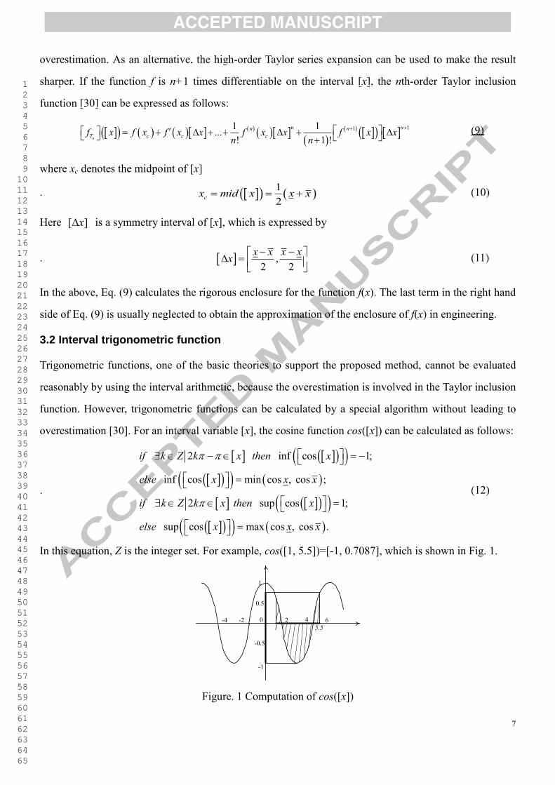
overestimation [30]. For an interval variable [x], the cosine function cos([x]) can be calculated as follows:

.

2 inf cos 1;

inf cos min cos , cos ;

2 sup cos 1;

sup cos max cos , cos .

if k Z k x then x

else x x x

if k Z k x then x

else x x x

(12)

In this equation, Z is the integer set. For example, cos([1, 5.5])=[-1, 0.7087], which is shown in Fig. 1.

2 4 60-2-4

-1

-0.5

0.5

1

1 5.5

Figure. 1 Computation of cos([x])

1 2 3 4 5 6 7 8 9 10 11 12 13 14 15 16 17 18 19 20 21 22 23 24 25 26 27 28 29 30 31 32 33 34 35 36 37 38 39 40 41 42 43 44 45 46 47 48 49 50 51 52 53 54 55 56 57 58 59 60 61 62 63 64 65

8

3.3 Chebyshev inclusion function

If the function f(x) is included in C[a, b], which means f(x) is continuous over [a, b], there exists a

polynomials p(x) which converges to the function f(x) on [a, b] [31], that is

. , ,f x p x x a b

(13)

This expression is validity for any 0 . Let Pn(x) denote the set of polynomials of degree not bigger

than n, for every nonnegative integer n, there exists a unique polynomial *np x in Pn(x), such that

. *n nf x p x f x p x E f

, where ,x a b (14)

For all np x P x other than *np x , nE f , the infimum of maximum error, is defined as

. infn n

n np P

E f f x p x

, where ,x a b (15)

Here *np x is the best uniform approximation of degree n to f(x) on [a, b]. However, it’s difficult to

obtain *np x when the degree of polynomials n>2. The truncate Chebyshev series are very close to the

best uniform approximation polynomials, which are employed to approximate the original function.

The Chebyshev polynomial for ,x a b of degree n is denoted by Cn and defined by [32]

. cosnC x n , where

2arccos 0,

x b ab a

(16)

where n denotes the nonnegative integer. The Chebyshev series can also be expressed as the polynomial

of -1,1x , and the recurrence relations are defined by

0 1

+1 -1

1, ,

2 -n n n

C x C x x

C x xC x C x

. (17)

For the multi-dimensional problem, the polynomials are the tensor product of each one-dimensional

polynomial, e.g. the k-dimensional Chebyshev polynomials of 1,1ix ( 1,2,...,i k ) is defined as:

. 1 2, ,..., 1 2 1 1 2 2, ,..., cos cos ...cos

kn n n k k kC x x x n n n (18)

where arccosi ix . It is noted that the one-dimensional problem with 1,1x is considered here

only for the consideration of simplicity without losing any generality. The Chebyshev series are orthogonal, such that

1 2 3 4 5 6 7 8 9 10 11 12 13 14 15 16 17 18 19 20 21 22 23 24 25 26 27 28 29 30 31 32 33 34 35 36 37 38 39 40 41 42 43 44 45 46 47 48 49 50 51 52 53 54 55 56 57 58 59 60 61 62 63 64 65

9

.

1

21 0

, 02, 0cos cos

1 0,

n m

m nC x C x

dx d m nn mx m n

(19)

where 21 1 x is the weighting function. The function f(x) included in C[a, b] can be approximated as

the truncate Chebyshev series of degree n:

. 01

12

n

n i ii

f x p x f f C x

(20)

where fi are the constant coefficients. The error between the truncated Chebyshev series pn(x) and original

function f(x) is shown as follow [33]:

.

121 !

nn

n ne f f x p x fn

(21)

In the above equation, if n is large enough, ne f can be neglected. The truncated Chebyshev series can

approximate the original function better than the truncated Taylor series, as shown by Example 1 as below.

Similar to the Taylor inclusion function, the Chebyshev inclusion function is defined by

. 0 01 1

1 1 cos2 2n

n n

C i i ii i

f x f f C x f f i

(22)

where[ ] [0, ] . It should be noted that Eq. (22) is not a rigorous inclusion function, because the error

term ne f is not incorporated in the function [ ]([ ])nCf x . Fortunately, in most cases the error can be

neglected, as the error is submerged in the overestimation induced by the lower terms. Since[ ] [0, ] ,

through the algorithm of interval trigonometric functions shown in Section 3.2, Eq. (22) can be calculated

easily. The Chebyshev inclusion function usually produces sharper result than the Taylor inclusion

function, which can be displayed by Example 1. Considering Eqs. (19) and (20), the constant coefficients fi can then be calculated by

.

1

21 0

2 2 cos cos1

ii

f x C xf dx f i d

x

, where 0,1,2,...,i n (23)

Eq. (23) will be calculated through numerical integral methods. Similarly, the multi-dimensional

coefficients can be calculated as follows:

.

1

1 2

1 1 ,...,, ,..., 12 21 1

1

2 ... ...1 ... 1

k

k

ki i

i i i k

k

f Cf dx dx

x x

x x

1 2 3 4 5 6 7 8 9 10 11 12 13 14 15 16 17 18 19 20 21 22 23 24 25 26 27 28 29 30 31 32 33 34 35 36 37 38 39 40 41 42 43 44 45 46 47 48 49 50 51 52 53 54 55 56 57 58 59 60 61 62 63 64 65

10

1 1 1 10 0

2 ... cos ,...,cos cos ...cos ...k

k k k kf i i d d

(24)

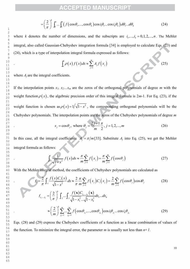
where k denotes the number of dimensions, and the subscripts are 1,..., 0,1,2,...,ki i n . The Mehler

integral, also called Gaussian-Chebyshev integration formula [34] is employed to calculate Eqs. (23) and

(24), which is a type of interpolation integral formula expressed as follows:

. 1

mb

j jaj

x f x dx A f x

(25)

where Aj are the integral coefficients. If the interpolation points x1, x2…xm are the zeros of the orthogonal polynomials of degree m with the

weight function x , the algebraic precision order of this integral formula is 2m-1. For Eq. (23), if the

weight function is chosen as 21 1x x , the corresponding orthogonal polynomials will be the

Chebyshev polynomials. The interpolation points are the zeros of the Chebyshev polynomials of degree m

. 2 1cos , where , 1,2,...,2j j j

jx j mm

(26)

In this case, all the integral coefficients jA m [33]. Substitute Aj into Eq. (25), we get the Mehler

integral formula as follows:

. 1

211 1

1 cos1

m m

j jj j

f x dx f x fm mx

(27)

With the Mehler integral method, the coefficients of Chebyshev polynomials are calculated as

.

1

211 1

2 2 2 cos cos1

m mi

i j i j j jj j

f x C xf dx f x C x f i

m mx

(28)

.

1

1

1 1 ,...,,..., 12 21 1

1

2 ... ...1 ... 1

k

k

ki i

i i k

k

f Cf dx dx

x x

x x

. 1 11

11 1

2 ... cos ,...,cos cos ...cosk k

k

k m m

j j j k jj j

f i im

(29)

Eqs. (28) and (29) express the Chebyshev coefficients of a function as a linear combination of values of

the function. To minimize the integral error, the parameter m is usually not less than n+1.

1 2 3 4 5 6 7 8 9 10 11 12 13 14 15 16 17 18 19 20 21 22 23 24 25 26 27 28 29 30 31 32 33 34 35 36 37 38 39 40 41 42 43 44 45 46 47 48 49 50 51 52 53 54 55 56 57 58 59 60 61 62 63 64 65

11

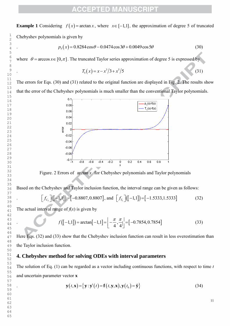
Example 1 Considering arctanf x x , where [ 1,1]x , the approximation of degree 5 of truncated

Chebyshev polynomials is given by

. 5 0.8284cos 0.0474cos3 0.0049cos5p x (30)

where arccos [0, ]x . The truncated Taylor series approximation of degree 5 is expressed by

. 3 55 3 5T x x x x (31)

The errors for Eqs. (30) and (31) related to the original function are displayed in Fig. 2. The results show

that the error of the Chebyshev polynomials is much smaller than the conventional Taylor polynomials.

Figure. 2 Errors of arctan x for Chebyshev polynomials and Taylor polynomials

Based on the Chebyshev and Taylor inclusion function, the interval range can be given as follows:

. 5

1,1 0.8807,0.8807Cf , and 5

1,1 1.5333,1.5333Tf (32)

The actual interval range of f(x) is given by

. 1,1 arctan 1,1 , 0.7854,0.78544 4

f

(33)

Here Eqs. (32) and (33) show that the Chebyshev inclusion function can result in less overestimation than

the Taylor inclusion function.

4. Chebyshev method for solving ODEs with interval parameters

The solution of Eq. (1) can be regarded as a vector including continuous functions, with respect to time t

and uncertain parameter vector x

. 0, : , , ,t t t t y x y y f y x y y (34)

1 2 3 4 5 6 7 8 9 10 11 12 13 14 15 16 17 18 19 20 21 22 23 24 25 26 27 28 29 30 31 32 33 34 35 36 37 38 39 40 41 42 43 44 45 46 47 48 49 50 51 52 53 54 55 56 57 58 59 60 61 62 63 64 65

12

Expanding Eq. (20) to a k-dimensional expression, the approximation of the vector y with respect to the

uncertain parameter vector x can be given as

. 1 1

1

,..., ,...,0 0

1, ...2 k k

k

pn n

i i i ii i

t C

y x y x (35)

where p denotes the total number of zero(s) to be occurred in the subscripts 1,..., ki i , 1 ,..., ki iC x is the

k-dimensional Chebyshev polynomials given in Eq. (18), and 1 ,..., ki iy denotes the vector including the

coefficients of Chebyshev polynomials. The Chebyshev polynomials are only the function of x, so the

coefficients vector 1 ,..., ki iy is the function of time t.

Consider Eq. (29), the coefficients are calculated by

. 1 1 11

,..., 11 1

2 ... ,cos ,...,cos cos ...cosk k k

k

k m m

i i j j j k jj j

t i im

y y (36)

where j denotes the zeros of Chebyshev polynomials with degree m, as shown in Eq. (26). With Eq.

(34), if the uncertain parameter vector is chosen as 1

[cos ,...,cos ]kj j x ,

1( ,cos ,...,cos )

kj jt y in the

above equation will be the solution of Eq. (1). As a result, any conventional numerical methods can be

applied to solve the differential equations. Substituting Eq. (36) into Eq. (35), and using the concept of

interval arithmetic, the interval solution of Eq. (1) can then be obtained. In a briefly description, the proposed method can transform the original each differential equation with

interval parameters into several differential equations of deterministic without any interval parameters.

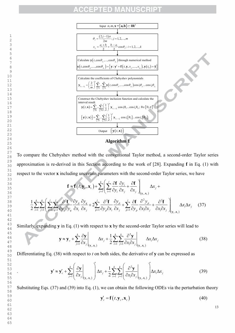
The detailed algorithm of the Chebyshev method can be described as Algorithm 1, which involves four

main steps: (1) to produce the interpolation points through Eq. (26), (2) to solve the differential equations

at the interpolation points to calculate y, (3) to calculate the coefficients of Chebyshev polynomials by Eq.

(29), and (4) to construct the Chebyshev inclusion function and obtain the corresponding interval [y]. From Algorithm 1, we find that the algorithm solving the uncertain problem is similar to a type of

sampling method, but the sampling points (interpolation points) have been defined in advance and the

post-processing are particular. Thus, the proposed method may be used to solve other uncertain dynamic

problems. For example, solving the ODEs system in the third step may be replaced by solving the

algebraic system, DAEs system, or even PDEs system, and then this theory would solve uncertain

multibody systems [35] and uncertain structure systems, and so on. However, the accuracy and efficiency

should be researched further.

1 2 3 4 5 6 7 8 9 10 11 12 13 14 15 16 17 18 19 20 21 22 23 24 25 26 27 28 29 30 31 32 33 34 35 36 37 38 39 40 41 42 43 44 45 46 47 48 49 50 51 52 53 54 55 56 57 58 59 60 61 62 63 64 65

13

Input , , kn m x = a,b IR

2 1; 1,2,...,

2

cos ; 1,2,...,2 2i

j

i i i ij j

jj m

ma b b ax i k

Calculate through numerical method

1 0,cos ,...,cos : , , ,..., ,k i kj j j jt t x x t y y y f y y y

Calculate the coefficients of Chebyshev polynomials

1 1 11

,..., 11 1

2 ... ,cos ,...,cos cos ...cosk k k

k

k m m

i i j j j k jj j

t i im

y y

Construct the Chebyshev inclusion function and calculate the interval result

1

1

11

,..., 1 10 0

,..., 1 10 0

1, ... cos θ ...cos θ ; θ 0,2

1, ... cos θ ...cos θ ;2

kk

kk

pn nk

i i k ki i

pn n

i i k ki i

t i i

t i i

y x y

y x y

1, cos ,..., cos

kj jt y

Output ,t y x

Algorithm 1

To compare the Chebyshev method with the conventional Taylor method, a second-order Taylor series

approximation is re-derived in this Section according to the work of [28]. Expanding f in Eq. (1) with

respect to the vector x including uncertain parameters with the second-order Taylor series, we have

1 1,

, ,c c

k li

c c jj i i j j

yt xy x x

y x

f ff f y x

22 2 2

1 1 1 1 1 1,

1 22

c c

k k l l l lp q p p

i ji j p q p pp q i j p i j p i j i j

y y y yx x

y y x x y x x y x x x x

y x

f f f f (37)

Similarly, expanding y in Eq. (1) with respect to x by the second-order Taylor series will lead to

2

1 1 1, ,

12

c c c c

k k k

c j i jj i jj i j

x x xx x x

y x y x

y yy y (38)

Differentiating Eq. (38) with respect to t on both sides, the derivative of y can be expressed as

.

2

1 1 1, ,

12

c c c c

k k k

c j i jj i jj i j

x x xx x x

y x y x

y yy y (39)

Substituting Eqs. (37) and (39) into Eq. (1), we can obtain the following ODEs via the perturbation theory

, ,c c ct y f y x (40)

1 2 3 4 5 6 7 8 9 10 11 12 13 14 15 16 17 18 19 20 21 22 23 24 25 26 27 28 29 30 31 32 33 34 35 36 37 38 39 40 41 42 43 44 45 46 47 48 49 50 51 52 53 54 55 56 57 58 59 60 61 62 63 64 65

14

1, ,c c c c

li

ij i j j

yx y x x

y x y x

y f f (41)

22 2 2 2

1 1 1 1, ,

2c c c c

l l l lp q p p

p q p pi j p q i j p i j p i j i j

y y y yx x y y x x y x x y x x x x

y x y x

y f f f f (42)

where , 1,...,i j k . Solving the ODEs given from Eq. (40) to Eq. (42) and then substituting the solutions

into Eq. (38), the interval solution of y can be obtained. Both the Chebyshev and Taylor methods transform the ODEs with uncertain parameters into new ODEs

with deterministic parameters. However, the expression of ODEs obtained with the Taylor method is

different from the original ODEs, while the Chebyshev method keeps the expression of the original ODEs

unchanged. Thus, the Chebyshev method is more convenient in the numerical implementation.

5. Numerical examples

The algorithms for the Chebyshev and Taylor methods are programmed using MATLAB tool: INTLAB

[36]. This paper is mainly focused on the presentation of a new interval analysis methodology to solve

uncertain problems of nonlinear dynamic systems. Two numerical examples have been carefully chosen

to demonstrate the effectiveness of the proposed method. Both examples include nonlinear elements, in

particular the pendulum mechanism model which is highly nonlinear. The results obtained by the

Chebyshev and Taylor methods are compared with the results of the scanning method [37].

5.3.1 Vehicle ride analysis

A two-degree-of-freedom quarter-car model [38] is shown in Fig. 3.

ms

mu

kscs

kt

xr

xu

xs

v

Figure. 3 Two-degree-of-freedom quarter car model

1 2 3 4 5 6 7 8 9 10 11 12 13 14 15 16 17 18 19 20 21 22 23 24 25 26 27 28 29 30 31 32 33 34 35 36 37 38 39 40 41 42 43 44 45 46 47 48 49 50 51 52 53 54 55 56 57 58 59 60 61 62 63 64 65

15

The cubic nonlinear characteristic of the spring stiffness can be expressed as follows:

.

3

3

s s s u s s u

t t u r t u r

F k x x K x x

F k x x K x x

(43)

where Fs and Ft denote the suspension force and tyre force, ks and kt are the linear stiffness characteristics

of the suspension and tyre, and Ks and Kt represent the cubic stiffness characteristics of the suspension and

tyre, respectively. The differential equations of the system motion model are expressed as follows:

.

3

3 3

0

0s s s s u s s u s s u

u u s s u s s u s s u t u r t u r

m x c x x k x x K x x

m x c x x k x x K x x k x x K x x

(44)

The initial condition for the above problem are given as: 0( ) 0sx t , 0( ) 0ux t , 0( ) 0sx t and

0( ) 0ux t . Here, ms, mu, and cs are the sprung mass, unsprung mass, and suspension damping rate,

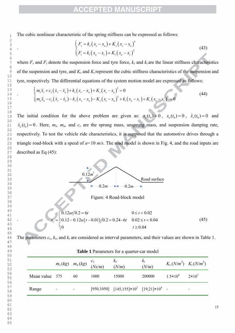
respectively. To test the vehicle ride characteristics, it is supposed that the automotive drives through a

triangle road-block with a speed of u=10 m/s. The road model is shown in Fig. 4, and the road inputs are

described as Eq (45):

0.12m

0.2m 0.2mRoad surface

Figure. 4 Road-block model

.

0.12 0.2 6 0 0.020.12 0.12 0.01 0.2 0.24 - 6 0.02 0.040 0.04

r

ut t tx u t t t

t

(45)

The parameters cs, ks, and kt are considered as interval parameters, and their values are shown in Table 1.

Table 1 Parameters for a quarter-car model

ms (kg) mu (kg) cs

(Ns/m) ks

(N/m) kt

(N/m) Ks (N/m3) Kt (N/m3)

Mean value 375 60 1000 15000 200000 1.5×106 2×107

Range - - [950,1050] [145,155]×102 [19,21]×104 - -

1 2 3 4 5 6 7 8 9 10 11 12 13 14 15 16 17 18 19 20 21 22 23 24 25 26 27 28 29 30 31 32 33 34 35 36 37 38 39 40 41 42 43 44 45 46 47 48 49 50 51 52 53 54 55 56 57 58 59 60 61 62 63 64 65

16

To solve the second-order ODEs, Eq. (44) is transformed into the following first-order ODEs

3

3 3

1

1

s s

u u

s s s u s s u s s us

u s s u s s u s s u t r u t r uu

x vx v

v c v v k x x K x xm

v c v v k x x K x x k x x K x xm

(46)

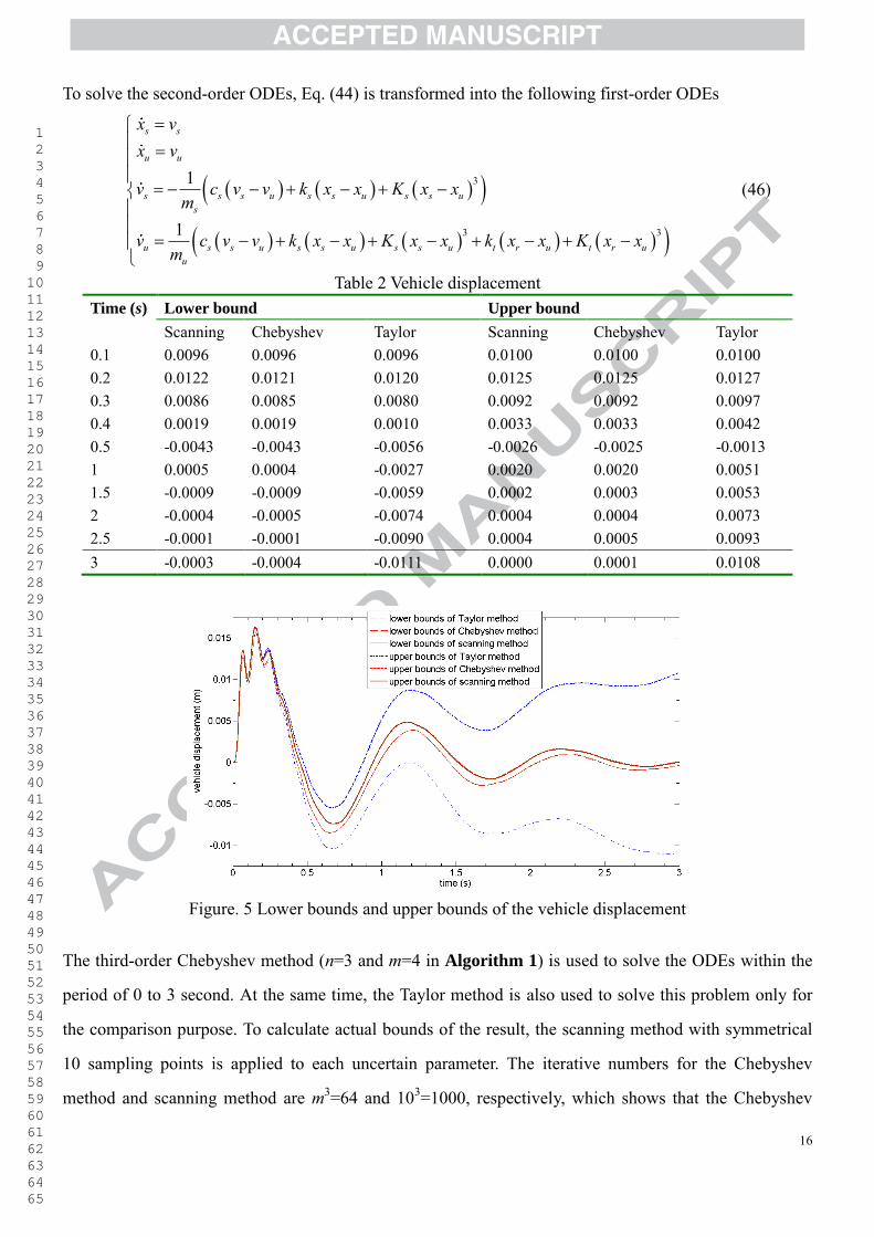
Table 2 Vehicle displacement Time (s) Lower bound Upper bound

Scanning Chebyshev Taylor Scanning Chebyshev Taylor 0.1 0.0096 0.0096 0.0096 0.0100 0.0100 0.0100 0.2 0.0122 0.0121 0.0120 0.0125 0.0125 0.0127 0.3 0.0086 0.0085 0.0080 0.0092 0.0092 0.0097 0.4 0.0019 0.0019 0.0010 0.0033 0.0033 0.0042 0.5 -0.0043 -0.0043 -0.0056 -0.0026 -0.0025 -0.0013 1 0.0005 0.0004 -0.0027 0.0020 0.0020 0.0051 1.5 -0.0009 -0.0009 -0.0059 0.0002 0.0003 0.0053 2 -0.0004 -0.0005 -0.0074 0.0004 0.0004 0.0073 2.5 -0.0001 -0.0001 -0.0090 0.0004 0.0005 0.0093 3 -0.0003 -0.0004 -0.0111 0.0000 0.0001 0.0108

Figure. 5 Lower bounds and upper bounds of the vehicle displacement

The third-order Chebyshev method (n=3 and m=4 in Algorithm 1) is used to solve the ODEs within the

period of 0 to 3 second. At the same time, the Taylor method is also used to solve this problem only for

the comparison purpose. To calculate actual bounds of the result, the scanning method with symmetrical

10 sampling points is applied to each uncertain parameter. The iterative numbers for the Chebyshev

method and scanning method are m3=64 and 103=1000, respectively, which shows that the Chebyshev

1 2 3 4 5 6 7 8 9 10 11 12 13 14 15 16 17 18 19 20 21 22 23 24 25 26 27 28 29 30 31 32 33 34 35 36 37 38 39 40 41 42 43 44 45 46 47 48 49 50 51 52 53 54 55 56 57 58 59 60 61 62 63 64 65

17

method spends less computational time than the scanning method. The vehicle displacement is shown in

Fig. 5, and the other details are listed in Table 2. From Fig. 5 and Table 2, it can be found that the Taylor

method will gradually enlarge the interval range in the numerical process, while the Chebyshev method

can enclose the actual result tight in the entire numerical procedure.

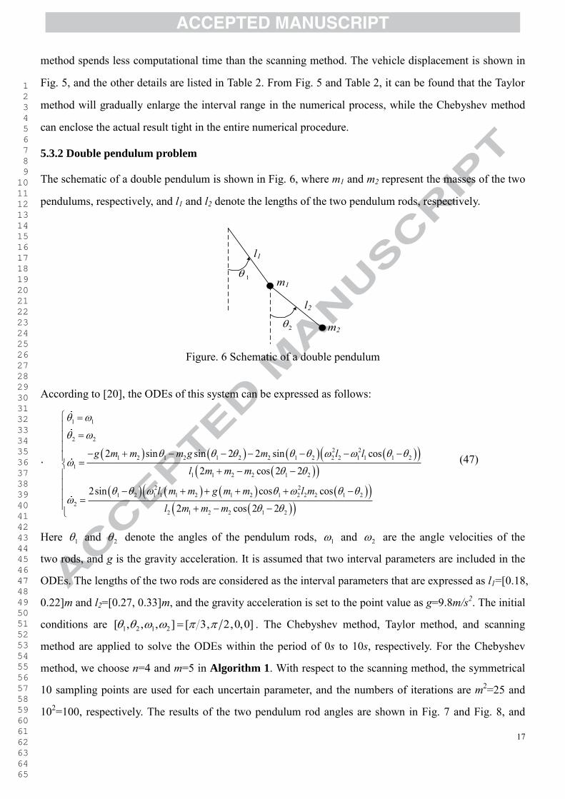
5.3.2 Double pendulum problem

The schematic of a double pendulum is shown in Fig. 6, where m1 and m2 represent the masses of the two

pendulums, respectively, and l1 and l2 denote the lengths of the two pendulum rods, respectively.

l1

1

l2

2

m1

m2

Figure. 6 Schematic of a double pendulum

According to [20], the ODEs of this system can be expressed as follows:

.

1 1

2 2

2 21 2 1 2 1 2 2 1 2 2 2 1 1 1 2

11 1 2 2 1 2

2 21 2 1 1 1 2 1 2 1 2 2 2 1 2

22 1 2 2 1 2

2 sin sin 2 2 sin cos2 cos 2 2

2sin cos cos2 cos 2 2

g m m m g m l ll m m m

l m m g m m l ml m m m

(47)

Here 1 and 2 denote the angles of the pendulum rods, 1 and 2 are the angle velocities of the

two rods, and g is the gravity acceleration. It is assumed that two interval parameters are included in the

ODEs. The lengths of the two rods are considered as the interval parameters that are expressed as l1=[0.18,

0.22]m and l2=[0.27, 0.33]m, and the gravity acceleration is set to the point value as g=9.8m/s2. The initial

conditions are 1 2 1 2[ , , , ] [ 3, 2,0,0] . The Chebyshev method, Taylor method, and scanning

method are applied to solve the ODEs within the period of 0s to 10s, respectively. For the Chebyshev

method, we choose n=4 and m=5 in Algorithm 1. With respect to the scanning method, the symmetrical

10 sampling points are used for each uncertain parameter, and the numbers of iterations are m2=25 and

102=100, respectively. The results of the two pendulum rod angles are shown in Fig. 7 and Fig. 8, and

1 2 3 4 5 6 7 8 9 10 11 12 13 14 15 16 17 18 19 20 21 22 23 24 25 26 27 28 29 30 31 32 33 34 35 36 37 38 39 40 41 42 43 44 45 46 47 48 49 50 51 52 53 54 55 56 57 58 59 60 61 62 63 64 65

18

more detailed results are shown in Table 3 and Table 4, respectively.

Figure. 7(a) The angle of top pendulum

Figure. 7(b) The angle of top pendulum removing the results of Taylor method

Table 3 The angle of top pendulum

Time

(s)

Lower bound Upper bound

Scanning Chebyshev Taylor Scanning Chebyshev Taylor 1 0.0405 0.0109 -0.0936 0.2229 0.2518 0.3551 2 -1.0818 -1.2651 -1.2526 -0.7598 -0.7575 -0.7693 3 -0.7636 -0.9644 -1.5272 0.2360 0.8083 1.1623 4 0.0622 -0.1984 -0.1822 1.0783 1.8313 1.7667 5 -0.6910 -0.9107 -1.2058 1.1097 1.6752 2.3863 6 -1.1744 -2.3797 -12.8006 0.3423 0.8866 11.4587 7 -1.1646 -2.5892 -84.5239 0.9261 2.2411 81.8147 8 -0.3745 -2.0719 -14.1746 1.2055 3.3500 14.7794 9 -1.1335 -2.886 -26.7229 1.1368 2.9360 28.2597

1 2 3 4 5 6 7 8 9 10 11 12 13 14 15 16 17 18 19 20 21 22 23 24 25 26 27 28 29 30 31 32 33 34 35 36 37 38 39 40 41 42 43 44 45 46 47 48 49 50 51 52 53 54 55 56 57 58 59 60 61 62 63 64 65

19

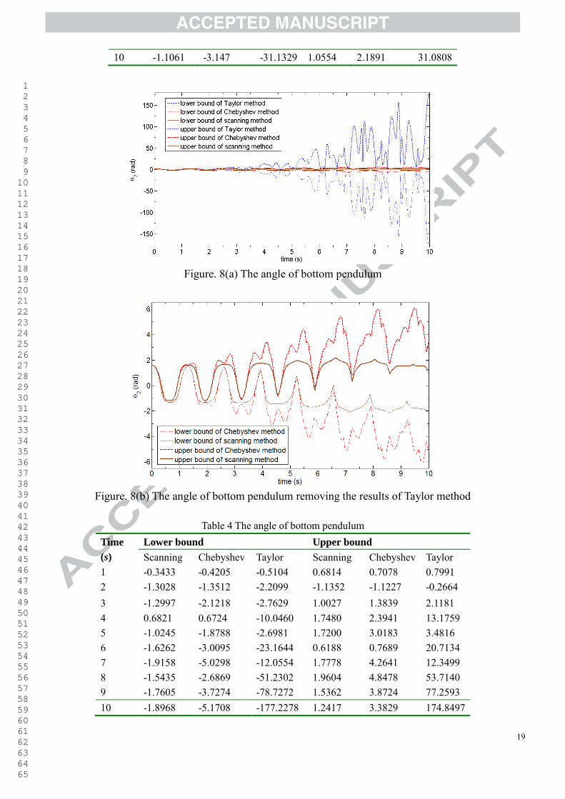
10 -1.1061 -3.147 -31.1329 1.0554 2.1891 31.0808

Figure. 8(a) The angle of bottom pendulum

Figure. 8(b) The angle of bottom pendulum removing the results of Taylor method

Table 4 The angle of bottom pendulum

Time

(s)

Lower bound Upper bound

Scanning Chebyshev Taylor Scanning Chebyshev Taylor 1 -0.3433 -0.4205 -0.5104 0.6814 0.7078 0.7991 2 -1.3028 -1.3512 -2.2099 -1.1352 -1.1227 -0.2664 3 -1.2997 -2.1218 -2.7629 1.0027 1.3839 2.1181 4 0.6821 0.6724 -10.0460 1.7480 2.3941 13.1759 5 -1.0245 -1.8788 -2.6981 1.7200 3.0183 3.4816 6 -1.6262 -3.0095 -23.1644 0.6188 0.7689 20.7134 7 -1.9158 -5.0298 -12.0554 1.7778 4.2641 12.3499 8 -1.5435 -2.6869 -51.2302 1.9604 4.8478 53.7140 9 -1.7605 -3.7274 -78.7272 1.5362 3.8724 77.2593 10 -1.8968 -5.1708 -177.2278 1.2417 3.3829 174.8497

1 2 3 4 5 6 7 8 9 10 11 12 13 14 15 16 17 18 19 20 21 22 23 24 25 26 27 28 29 30 31 32 33 34 35 36 37 38 39 40 41 42 43 44 45 46 47 48 49 50 51 52 53 54 55 56 57 58 59 60 61 62 63 64 65

20

From Figs. 7(a) and 8(a) and Tables 3 and 4, we can find that the Taylor method enlarges the range of

results along with the process of the iteration, while Chebyshev method can enclosure the actual results in

the entire numerical period without large overestimation. However, it is noted that there are still some

overestimation for the proposed Chebyshev method from Figs. 7(b) and 8(b), which cannot be totally

avoided when the interval arithmetic is applied to systems with high nonlinearity, except that additional

design optimization algorithms are incorporated, which will cost the computational effort.

6. Conclusions

A new interval method with the Chebyshev series has been proposed for the analysis of the dynamic

response of nonlinear systems with uncertain-but-bounded parameters. The truncated Chebyshev series

expansion is used to approximate the solution in a general way with higher accuracy than the truncated

Taylor series expansion, especially for non-monotonic solutions. The Chebyshev inclusion function,

based on the Chebyshev polynomials, has better ability to control the overestimation compared with the

conventional Taylor inclusion function. The Mehler numerical integral method is employed to calculate

the coefficients of Chebyshev polynomials. With the Chebyshv polynomials, the set of ODEs with

interval parameters are transformed to a new set of ODEs with deterministic parameters. Then, many

numerical methods for solving ODEs can be applied to obtain the solution. The second-order Taylor

method is also derived by using the perturbation theory, in order to compare with the Chebyshev method. Two typical numerical examples are used to demonstrate the effectiveness of the proposed methodology.

The numerical results show that the Chebyshev method can achieve a tighter enclosure of the results than

the Taylor method, with respect to the scanning method. The proposed Chebyshev method, therefore,

produces less overestimation when applied to solve nonlinear dynamic problems of ODEs. The proposed

interval method can be used to evaluate the dynamic response of nonlinear systems with relatively large

uncertainties. Another advantage of the proposed Chebyshev method is non-intrusive, which can be easily

processed in the numerical implementation, while the Taylor method is intrusive due to the demand of

additional efforts. Our ongoing research is to combine the proposed Chebyshev interval analysis method

with optimization algorithms to achieve more accurate results.

Acknowledgement

This research was partially supported by the National Natural-Science-Foundation-of-China (11172108),

and the Chancellor’s Research Fellowship (2032062), the University of Technology, Sydney (UTS).

1 2 3 4 5 6 7 8 9 10 11 12 13 14 15 16 17 18 19 20 21 22 23 24 25 26 27 28 29 30 31 32 33 34 35 36 37 38 39 40 41 42 43 44 45 46 47 48 49 50 51 52 53 54 55 56 57 58 59 60 61 62 63 64 65

21

Reference

[1] G.I. Schuëller, H.A. Jensen, Computational methods in optimization considering uncertainties - an overview, Computer Methods in Applied Mechanics and Engineering 198 (2008) 2-13. [2] Y. Ben-Haim, I. Elishakoff, Convex models of uncertainty in applied mechanics, Elsevier Science, Amsterdam, 1990. [3] M.A. Valdebenito, G.I. Schuëller, A survey on approaches for reliability-based optimization, Structural and Multidisciplinary Optimization 42 (2010) 645-663. [4] H.-G. Beyer, B. Sendhoff, Robust optimization - A comprehensive survey, Computer Methods in Applied Mechanics and Engineering, 196 (2007) 3190-3218. [5] H. Chen, Stability and chaotic dynamics of a rate gyro with feedback control under uncertain vehicle spin and acceleration, Journal of Sound and Vibration, 273 (2004) 949-968. [6] H. Cheng, A. Sandu, Uncertainty quantification and apportionment in air quality models using the polynomial chaos method, Environmental Modelling & Software, 24 (2009) 917-925. [7] M. Hanss, The transformation method for the simulation and analysis of systems with uncertain parameters, Fuzzy Sets and Systems, 130 (2002) 277-289. [8] W. Chen, R. Jin, A. Sudjianto, Analytical variance-based global sensityivity analysis in simulation-based design under uncertainty, Journal of Mechanical Design, 127 (2005) 875-886. [9] S.S. Isukapalli, A. Roy, P.G. Georgopoulos, Stochastic Response Surface Methods (SRSMs) for uncertainity propagation application to environmental and biological systems, Risk Analysis, 18 (1998) 351-363. [10] A. Sandu, C. Sandu, M. Ahmadian, Modeling Multibody Systems with Uncertainties. Part I: Theoretical and Computational Aspects, Multibody System Dynamics, 15 (2006) 369-391. [11] D. Xiu, G.E. Karniadakis, The Wiener-Askey polynomial chaos for stochastic differential equations, SIAM Journal on Scientific Computing, 24 (2002) 619-644. [12] X. Yin, S. Lee, W. Chen, W.K. Liu, M.F. Horstemeyer, Efficient Random Field Uncertainty Propagation in Design Using Multiscale Analysis, Journal of Mechanical Design, 131 (2009) 021006. [13] D. Moens, D. Vandepitte, A survey of non-probabilistic uncertainty treatment in finite element analysis, Computer Methods in Applied Mechanics and Engineering, 194 (2005) 1527-1555. [14] R.E. Moore, Interval analysis, Prentice-Hall, Englewood Cliffs, New Jersey, 1966. [15] H. Ishibuchi, H. Tanaka, Multiobjective programming in optimization of the interval objective function, European Journal of Operational Research, 48 (1990) 219-225. [16] N.S. Nedialkov, K.R. Jackson, G.F. Corliss, Validated solutions of initial value problems for odinary differential equations., Applied Mathematics and Computation, 105 (1999) 21-68. [17] K.R. Jackson, N.S. Nedialkov, Some recent advances in validated methods for IVPs for ODEs, Applied Mathematics and Computation, 42 (2002) 269-284. [18] G. Alefeld, G. Mayer, Interval analysis: theory and applications, Journal of Computational and Applied Mathmatics, 121 (2000) 421-464. [19] M. Berz, K. Makino, Efficient Control of the Dependency Problem Based on Taylor Model Methods, Reliable Computing, 5 (1999) 3-12. [20] Y. Lin, M.A. Stadtherr, Validated solutions of initial value problems for parametric ODEs, Applied Numerical Mathematics, 57 (2007) 1145-1162. [21] Z. Qiu, X. Wang, Comparison of dynamic response of structures with uncertain-but-bounded parameters using non-probabilistic interval analysis method and probabilistic approach, International Journal of Solids and Structures, 40 (2003) 5423-5439. [22] Z. Qiu, X. Wang, Parameter perturbation method for dynamic responses of structures with uncertain-but-bounded parameters based on interval analysis, International Journal of Solids and Structures, 42 (2005) 4958-4970. [23] J. Hu, Z. Qiu, Non-probabilistic convex models and interval analysis method for dynamic response of a beam with

1 2 3 4 5 6 7 8 9 10 11 12 13 14 15 16 17 18 19 20 21 22 23 24 25 26 27 28 29 30 31 32 33 34 35 36 37 38 39 40 41 42 43 44 45 46 47 48 49 50 51 52 53 54 55 56 57 58 59 60 61 62 63 64 65

22

bounded uncertainty, Applied Mathematical Modelling, 34 (2010) 725-734. [24] Z. Qiu, Two non-probabilistic set-theoretical models to predict the transient vibrations of cross-ply plates with uncertainty, Applied Mathematical Modelling, 32 (2008) 2872-2887. [25] J. Wu, Y. Zhao, S. Chen, An improved interval analysis method for uncertain structures, Structural Engineering and Mechanics, 20 (2005) 713-726. [26] X. Zhang, H. Ding, S. Chen, Interval finite element method for dynamic response of closed-loop system with uncertain parameters, International Journal for Numerical Methods in Engineering, 70 (2007) 543-562.

[27] X. Han, C. Jiang, S. Gong, Y.H. Huang, Transient waves in composite‐laminated plates with uncertain load and material

property, International Journal for Numerical Methods in Engineering, 75 (2008) 253-274. [28] Z. Qiu, L. Ma, X. Wang, Non-probabilistic interval analysis method for dynamic response analysis of nonlinear systems with uncertainty, Journal of Sound and Vibration, 319 (2009) 531-540. [29] K. Makino, M. Berz, Taylor models and other validated functional inclusion methods, International Journal of Pure and Applied Mathematics, 4 (2003) 379-456. [30] L. Jaulin, Applied interval analysis: with examples in parameter and state estimation, robust control and robotics, Springer, New York, 2001. [31] B. Erret, A Generalization of the Stone-Weierstrass theorem, Pacific Journal of Mathematics 11 (1961) 777-783. [32] T.J. Rivlin, An Introduction to the Approximation of Functions, Dover, New York, 1981. [33] E. Jiang, F. Zhao, Y. Shu, Numerical Approximation, Fudan University Press, Shanghai, 2008. [34] M. Abramowitz, I.A. Stegun, Handbook of Mathematical Functions with Formulas, Graphs, and Mathematical Tables, Dover, New York, 1972. [35] J.L. Wu, Y.Q. Zhang, The Dynamic Analysis of Multibody Systems with Uncertain Parameters Using Interval Method, Applied Mechanics and Materials, 152-154 (2012) 1555-1561. [36] G. Hargreaves, I, Interval analysis in MATLAB, in: Numerical Analysis Report, Manchester, 2002, pp. 1-49.

[37] A.J. Buras, M. Jamin, M.E. Lautenbacher, A 1996 Analysis of the CP. Violating Ratio ε′/ε, Physics Letters B, 389 (1996)

749-756. [38] W. Gao, J.C. Ji, N. Zhang, H.P. Du, Dynamic analysis of vehicles with uncertainty, Proceedings of the Institution of Mechanical Engineers, Part D: Journal of Automobile Engineering, 222 (2008) 657-664.