doi: 10.3319/TAO.2012.03.28.02(A)

* Corresponding author E-mail: kuo@as.ntu.edu.tw

Terr. Atmos. Ocean. Sci., Vol. 23, No. 4, 439-450, August 2012

A New Parallel Domain-Decomposed Chebyshev Collocation Method for Atmospheric and Oceanic Modeling

Yu-Ming Tsai1, Hung-Chi Kuo1, *, Yung-Chieh Chang 2, and Yu-Heng Tseng1

1 Department of Atmospheric Sciences, National Taiwan University, Taipei, Taiwan 2 Department of Applied Mathematics, National Chiao Tung University, Hsinchu, Taiwan

Received 19 July 2011, accepted 28 March 2012

AbstrACt

Spectral methods seek the solution to a differential equation in terms of series of known smooth function. The Chebyshev series possesses the exponential-convergence property regardless of the imposed boundary condition, and therefore is suited for the regional modeling. We propose a new domain-decomposed Chebyshev collocation method which facilitates an efficient parallel implementation. The boundary conditions for the individual sub-domains are exchanged through one grid interval overlapping. This approach is validated using the one dimensional advection equation and the inviscid Burgers’ equation. We further tested the vortex formation and propagation problems using two-dimensional nonlinear shallow water equations. The domain decomposition approach in general gave more accurate solutions compared to that of the single domain calculation. Moreover, our approach retains the exponential error convergence and conservation of mass and the quadratic quantities such as kinetic energy and enstrophy. The efficiency of our method is greater than one and increases with the number of processors, with the optimal speed up of 29 and efficiency 3.7 in 8 processors. Efficiency greater than one was obtained due to the reduc-tion the degrees of freedom in each sub-domain that reduces the spectral operational count and also due to a larger time step allowed in the sub-domain method. The communication overhead begins to dominate when the number of processors further increases, but the method still results in an efficiency of 0.9 in 16 processors. As a result, the parallel domain-decomposition Chebyshev method may serve as an efficient alternative for atmospheric and oceanic modeling.

Key words: Chebyshev collocation method, Domain-decomposition, 2-D nonlinear shallow water modelCitation: Tsai, Y. M., H. C. Kuo, Y. C. Chang, and Y. H. Tseng, 2012: A new parallel domain-decomposed Chebyshev collocation method for atmospheric and oceanic modeling. Terr. Atmos. Ocean. Sci., 23, 439-450, doi: 10.3319/TAO.2012.03.28.02(A)

1. INtrODuCtION

Advances in spectral transform methods (Orszag 1970) and Fast Fourier Transform (FFT) brought about success-ful global atmospheric modeling using these methods (e.g., Bourke et al. 1977; Machenhauer 1979). Compared with fi-nite difference and finite element (volume) methods, global spectral models with spherical harmonics can eliminate the singularity of poles and preserve high accuracy and effi-ciency due to the “exponential convergence” property and the easy implementation of the semi-implicit method. The spectral methods also allow the discrete conservation of ki-netic energy and enstrophy, which are important for two-dimensional turbulence.

In addition to the popularity of spectral methods for global models, the modified Fourier method is often used in operational regional spectral models, such as the fore-cast model at the Japan Meteorological Agency (Segami et al. 1989), US NCEP regional spectral model (Juang and Kanamitsu 1994; Juang 2000), and the HIgh-Resolution Limited-Area Model (HIRLAM) in Europe (Haugen and Machenhauer 1993). However, the exponential conver-gence property in these models may reduce to algebraic convergence with O(N -3), which loses the major advantage of the Fourier method. Also, the basis functions used in the modified Fourier method need to be determined by the time-dependent boundary conditions and cannot be selected arbitrarily (Roache 1978; Kuo and Williams 1992; Adcock 2009).

Tsai et al.440

Fulton and Schubert (1987a, b) proposed a Chebyshev spectral method for the limited area (regional) atmospheric modeling. The method successfully handles the time-depen-dent boundary conditions while retaining the advantage of spectral method. The appeal of Chebyshev spectral meth-ods in the regional atmospheric modeling is its efficiency and accuracy due to the fast transform, and the exponential convergence rate for the selected basis function. The con-vergence rate of the Chebyshev method depends mainly on the smoothness of the expanded function, rather than the boundary conditions (Fulton and Schubert 1987a; Kuo and Williams 1992, 1998). Moreover, Chebyshev transforms can be implemented using FFT since they can be reduced to discrete cosine transforms (Fulton and Schubert 1987a; Kopriva 2009).

There are two types of projections for Chebyshev spectral modeling. In the tau approximation, the Chebyshev basis functions need not individually satisfy the boundary conditions; however, these boundary conditions are satis-fied by the whole truncated series. The other is called col-location projection, which requires the residual to vanish on the collocation points and the boundary conditions are implemented in physical space. Kuo and Schubert (1988) studied the stability of cloud-topped boundary layer with a Fourier-Chebyshev tau method based Boussinesq nonhy-drostatic convective model. The method handles the strong gradients of temperature and moisture which are critical in boundary layer convection modeling.

The idea of maintaining the exponential convergence property with domain-decomposition for spectral meth-ods was initiated by Patera (1984). Patera (1984) used the “Patched” method, in which each block spans a single in-terface line between a pair of adjoin domains, to handle the domain interface. Kopriva (1986, 1989) further proposed another composite-grid approach which maps the hyper-bolic equations in the complicated geometries to several squared sub-domains. The spectral method is performed within each domain. The advantages of domain-decompo-sition for Chebyshev spectral method were discussed in Ko-priva (1986, 1989) introduced both “patched” and “overset” methods for solving hyperbolic equations for complicated geometry. A decade later, Kopriva and Kolias (1996) de-veloped a conservative staggered-grid Chebyshev multi-domain method for compressible flows with patched grids. Kopriva (1996) found that within each sub-domain, the polynomial order can be determined independently regard-less of its neighbors. The Chebyshev pseudospectral (collo-cation) method with domain-decomposition is also applied to deal with viscous flow in order to reduce the Gibbs phe-nomena over an entire domain (Yang and Shizgal 1994). These Chebyshev-type spectral approaches with domain-decomposition problems such as hyperbolic equations (Ko-priva 1986, 1989), viscous flow (Yang and Shizgal 1994), and compressible flow (Kopriva 1996; Kopriva and Kolias

1996). However, none has directly applied to atmospheric modeling.

The spectral method with domain-decomposition can be regarded as a variation of “spectral element method” (Deville et al. 2002; Washington and Parkinson 2005; Clau-dio et al. 2007). One of the typical spectral element meth-ods is the discontinuous Galerkin method with Legendre polynomials (Iskandarani et al. 1995; Cockburn 2003; Ramachandran et al. 2005). The major advantage of the discontinuous Galerkin method is that much of the com-putation is local to an element and the conservation prop-erty is maintained. The Galerkin method is also suitable to simulate complex domain geometry. However, the compu-tational cost is expensive due to the spectral element and its parallel implementation requires better load balance. The unique benefit of Chebyshev spectral method lies in its fast transformation (Fulton and Schubert 1987a; Kopriva 2009), which is readily available and efficient. The Chebyshev spectral method uses the non-uniform (Chebyshev) grids with finer resolution near the boundary. It should be noted that equidistant grid points do not guarantee uniform error distribution (Runge phenomenon; Hesthaven et al. 2007), while Chebyshev grids provide uniform error distribution (Fig. 2.3 in Conte and Boor 1980). In addition, the domain-decomposition enhances the homogeneity of the fine resolu-tion as the number of sub-domains increases, which provide more flexibility for further adaptive grid refinement. Thus, the domain-decomposition approach adds the Chebyshev spectral method to the list of spectral element methods.

The traditional domain-decomposition method for Chebyshev spectral modeling is the “Patched” method which overlaps one grid point on the boundary. The numeri-cal flux is calculated from the left and right of the bound-ary to implement the sub-domain boundary condition (Ko-priva 2009). However, this process is complicated as (8.41) and (8.42) in Kopriva (2009). In this study, we follow the CReSS model (Tsuboki and Sakakibara 2002) method, which simply overlaps one-grid width, to exchange bound-ary information along the sub-domain boundaries. The 1-D advection equation, inviscid Burgers’ equation, and the 2-D fully nonlinear shallow water equations are used to check the validity of this new approach.

The main objective of this study is to develop and im-plement a new parallel Chebyshev collocation method with domain-decomposition which is suited for atmospheric and oceanic modeling. The multi-dimensional domain-decom-position provides the most flexible combination and effec-tive performance for the large-scale atmospheric and oce-anic modeling. The spectral operation counts for derivative computation are even reduced for each sub-domain, which leads to a high speed up value. Following the suggestion of Fulton and Schubert (1987a), we have adopted the shal-low water equations in advective form for better accuracy. Because the domain-decomposition is the most efficient

Domain-Decomposed Chebyshev Collocation Method 441

way in parallel computing to improve the computational efficiency, we employed Message Passing Interface (MPI) in this study. The multi-domain calculations are performed using different computing processes simultaneously, which reduces a significant amount of computing time and relieves the memory requirement for a large-scale system from the advantage of parallel computing (Smith et al. 1996; Shonk-wiler and Lefton 2006).

This paper is organized as follows. Section 2 introduc-es the Chebyshev collocation method. The parallel domain-decomposed Chebyshev collocation method is proposed in section 3. Section 4 investigates the accuracy of the parallel domain-decomposed Chebyshev method using advection and inviscid Burgers’ equations. The characteristics are discussed in terms of the exponential convergence of error. Section 5 presents the application of vortex formation and propagation using the 2-D nonlinear shallow water equa-tions. Finally, concluding remarks are given in section 6.

2. MethODs

Spectral methods seek solutions in terms of a series of known basis functions. The essence of choosing basis func-tions is based on the property of “completeness.” Namely, the solution can be represented by a set of functions. Practi-cal consideration of the basis functions for spectral methods is orthogonality and efficient calculation of their projection or inner product. The “orthogonality” of basis functions for spectral methods is practically important in the computation since the coefficients are independent.

Consider the Sturm-Liouville equation in the limited domain [a, b],

L x p x x q x x w x x{ { { m {= - + =l l^ ^ ^ ^ ^ ^ ^h h h h h h h6 @ (1)

where L is a linear operator involving space derivatives, with determined functions p(x), q(x), and w(x) . The prime represents the differentiation with respect to x. Equation (1) has infinite and countable sets of solutions x

n 0{ 3

=^ h , corre-sponding to their eigenvalues n 0m

3= . Therefore, any smooth

function u(x) can be expanded by the basis n n 0{ 3

=" , with ap-propriate coefficients as

u x u xn n n0 {= 3

= t^ ^h h/ (2)

where

,u un n w{=t ^ h (3)

To estimate the magnitude of unt , we substitute n{ in un =t,u n w{^ h from Eq. (1) and implement the integration by parts

twice:

, , ,u u w L B u vn n n n n n ww

1 1 1m { m { {= = +- - -t ^ ^ ^h h h6 @ (4)

where ,B u xp x u x u x xn n n x ax b{ { {= - =

=l l^ ^ ^ ^ ^ ^h h h h h h6 @ and v = w-1 Lu.

The Chebyshev polynomials are the solutions of Chebyshev differential equation which is a special case of the Sturm-Liouville equation with p(x) = (1 - x2)1/2, q(x) = 0 and w(x) = (1 - x2)-1/2. Taking the case having the domain [-1,1] and p(-1) = p(1) = 0, which means B(u, n{ ) equals to 0 no matter what bounded function u is, we can perform integration by parts for the ,vn n w

1m {- ^ h6 @ term repeatedly as long as the function is smooth enough after each inte-gration. Since the (v, n{ )w term is bounded regardless of n and the asymptotic behavior of eigenvalues λn = O(n2) and eigenvectors x O 1n{ =^ ^h h, x O nn{ =l^ ^h h as n " 3, we get u <nt O(n -m) if u is m times differentiable (Courant and Hilbert 1953). This indicates the exponential convergence by definition, i.e., the convergence rate of Chebyshev series only depends on the smoothness of the expanded function regardless of the boundaries. A thorough description of the Chebyshev spectral method is given in Fulton and Schu-bert (1987a, b). If a function is expanded by the truncated Chebyshev series Tn(x)

x T xnN

n n0} }= =t^ ^h h/ (5)

we can obtain the spectral coefficients n}t by the relation

, , , , ...c T n2 0 1nn

n}r}= =t ^ h (6)

where cn = 2 when n = 0, and cn = 1 when n > 0. Equa-tions (5) and (6) can be calculated efficiently by the Fast Chebyshev Transform. Similar to the Fast Fourier Trans-form, the Fast Chebyshev Transform reduces the N degree of freedom transformation to O(N log N) operations instead of O(N2) (Fulton and Schubert 1987a; Kopriva 2009). This advantage favors its potential application in large-scale at-mospheric modeling. Note that Chebyshev spectral method is known as the best method to reduce the point-wise error compared to other polynomial projection methods. It can also eliminate the wild oscillations near the boundary, so called Runge phenomena (i.e., Hesthaven et al. 2007).

3. the PArAllel DOMAIN-DeCOMPOsItION APPrOACh

The development of a parallel domain-decomposi-tion approach for Chebyshev collocation method is novel in atmospheric and oceanic modeling. The computational saving is significant not only due to the distributed com-puting for each domain, but also due to the relaxation for

Tsai et al.442

time constraint (i.e., allowing larger Δt), as mentioned in Kopriva (1986). For a limited domain with a specified de-gree of freedom N, the time step Δt is mainly constrained by the Courant-Friedrichs-Lewy (CFL) criteria. For the non-uniform Chebyshev grid, the minimal Δx is proportional to L/N2, where L is the length of the domain, N is the degrees of freedom. Assuming Δts and Δtm are the ideal time steps for certain numerical methods in a single domain and m domain-decomposed sub-domains, respectively, the propor-tionality of time step to the minimal Δx leads to

t NL

s 2\D (7)

and, similarly,

t N mL m

m NL

m 22\D =^ h (8)

where L/m is the length of each sub-domain and the minimal Δx in sub-domains is proportional to 1 / (N/m)2 (each sub-domain includes only N/m Chebyshev grids). This implies that an m time larger time step can be used when several sub-domains are employed. Ideally, this should result in an m2 speed-up in the distributed platform if no communication cost is taken into account. Apparently, the main advantage of domain-decomposition also favors the use of Chebyshev method.

Minimal communication between sub-domains is re-quired for an efficient atmospheric or oceanic model. Fol-lowing the grid arrangement of the CReSS model (Tsuboki and Sakakibara 2002), a one-grid width overlapped bound-aries is used here for the data exchange between sub-do-mains. Figure 1 shows the (a) one-dimensional and (b) two-dimensional schematic diagrams for the data exchange along the overlapped boundaries. Note that the grids setting match well at the overlapped boundaries. Assuming xMN to be the N th Chebyshev collocation point at M th sub-domain, we assign the data value u xMNa^ h to u x M 1 N+^ ^ hh and assign u x M 1 N Na+ -^ ^ ^ hh h to u xM0^ h, respectively. The length of each sub-domain is

cosL N N N NL

1 2 1 1aD D ar

= - - -^ ^ ^h h h6 @ (9)

where L is the length of the whole domain, Na + 1 is the num-ber of overlapped grids between sub-domains with Na ≥ 1, ND is the number of sub-domains, and N is the degrees of freedom of each sub-domain.

4. test PrObleMs

In order to show the accuracy and convergence of the

new domain-decomposed Chebyshev approach, we first consider the 1-D linear advection equation in the domain [-1, 1]

tu

xu 0

22

22+ = (10)

The initial and boundary conditions are given by the analyti-cal solution

, expu x t A hx x t0

2

= - - -^ `h j8 B (11)

where h = 0.2, x0 = -0.5 and A = h-1/2 (π / 2) -1/4 are selected as in Fulton and Schubert (1987a). The fourth-order Runge-Kutta method is used for the time integration scheme. Here, we also compare our results with the fourth-order finite dif-ference scheme (FD4).

Figure 2 compares the analytical solution and the nu-merical approximation by Chebyshev collocation method and FD4 at time t = 1.0 The domain is divided into two sub-domains with one grid width overlapping, e.g., two over-lapped grids, as shown in Fig. 1a. The degrees of freedom

Fig. 1. Schematic representation of (a) one-dimensional and (b) two-dimensional domain-decomposition and the communication strategy for parallel computations using MPI. The blue shadings represent the overlapped areas (after Tsuboki and Sakakibara 2002).

(a)

(b)

Domain-Decomposed Chebyshev Collocation Method 443

of each sub-domain is now 12. Figure 2a shows that the ap-proximation of Chebyshev collocation method with domain-decomposition is almost identical to the analytical solution in 1-D advection problem without numerical dispersion. Figure 2b further shows the L2 error of the numerical re-sults of Chebyshev collocation method with single domain, double domain, and FD4 method with analytical solution at t = 1.0. As expected, the absolute accuracy is slightly higher in the single domain than the double domains since the ad-vected Gaussian function is centered at x = 0.5, where the double domains have coarser resolution. However, the error convergence in the spectral solutions are uniformly decreas-ing on the order of 10 (-N/4) as N approaches 64, while the error in FD4 decreases on the order of N. The exponential convergence of the spectral method remains regardless of the number of domains. Instead of reproducing the identical result as single domain, the Chebyshev domain decomposi-tion approach shows the numerical convergence (converg-ing to the true solution) when we refine the resolution.

Next, we consider the inviscid Burgers’ equation in the limited domain [-1, 1]

tu u x u

x 022

22+ =^ h (12)

with the initial condition , tanu x u x x0 10= - --^ ^h h. The

boundary conditions are given by the general solution of Eq. (12). Thus, the analytical solution gives

tanu u x ut x10= - - -- ^ h (13)

Furthermore, the time of scale-collapse can be obtained by

differentiating Eq. (13) with respect to x

xu

x x utt u x

11

022

2 2 2= - + - -

-^^

hh

Assuming x x ut0= + and uu = , this gives

xu t x

u1x x ut x x ut0 02

222= - -

= + = +` `j j; E (14)

and then

xu

t t11 1as

x x ut0

" "22 3= - -

= +` j (15)

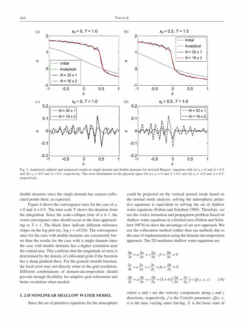
Thus, the time of scale-collapse of u is 1 with the position of scale-collapse at x u0 + . Given the appropriate u and x0, the analytical solution of Eq. (12) at certain x and t can be obtained numerically for desired accuracy. The fourth-order Runge-Kutta method is used for the time integration scheme. Figure 3a shows the numerical results compared with the analytical solution for the case .u 0 5= and x0 = 0 (the scale-collapse occurs at x0 = 0). The general pattern can be obtained by the numerical solution with only 32 de-grees of freedom. Figure 3c shows the corresponding er-ror distribution in the physical space. Note that the error in double domains is larger than that in single domain since the scale collapse (sharp front) is located near coarser col-located points. On the other hand, for another case .u 0 5= and x0 = -0.5, the scale collapse occurs near the center of the simulation domain (Fig. 3b), better results are achieved for

Fig. 2. (a) Comparison between the analytical solution (exact) and numerical results for the linear advection equation. Label “D” represents the Chebyshev collocation method with double domains. The result with the fourth-order finite difference scheme (FD4) is also superimposed. (b) The L2 error for FD4 and Chebyshev collocation method using single domain (S) and double domain (D), respectively.

(a) (b)

Tsai et al.444

double domains since the single domain has coarser collo-cated points there, as expected.

Figure 4 shows the convergence rates for the case of x0 = 0 and .u 0 5= . The time scale T shows the duration from the integration. Since the scale-collapse time of u is 1, the worst convergence rates should occur as the time approach-ing to T = 1. The black lines indicate different reference slopes on the log plot (mn: log y = nN/24). The convergence rates for the case with double domains are consistently bet-ter than the results for the case with a single domain since the case with double domains has a higher resolution near the central area. This confirms that the magnitude of error is determined by the density of collocated grids if the function has a sharp gradient there. For the general smooth function, the local error may not directly relate to the grid resolution. Different combinations of domain-decomposition should provide enough flexibility for adaptive grid refinement and better resolution when needed.

5. 2-D NONlINeAr shAllOw wAter MODel

Since the set of primitive equations for the atmosphere

could be projected on the vertical normal mode based on the normal mode analysis, solving the atmospheric primi-tive equations is equivalent to solving the set of shallow water equations (Fulton and Schubert 1985). Therefore, we use the vortex formation and propagation problem based on shallow water equations in a limited-area (Fulton and Schu-bert 1987b) to show the advantage of our new approach. We use the collocation method (rather than tau method) due to the ease of implementation using the domain-decomposition approach. The 2D nonlinear shallow water equations are

tu u u v y

u fv xh

x 022

22

22

22+ + - + =

0tv u x

v v yv fu y

h22

22

22

22+ + + + =

Q= , ,th u x

h v yh h h x

uyv x y t

22

22

22

22

22+ + + + +^ c ^h m h (16)

where u and v are the velocity components along x and y directions, respectively, f is the Coriolis parameter, Q(x, y, t) is the time varying outer forcing, h is the basic state of

Fig. 3. Analytical solution and numerical results in single domain and double domains for inviscid Burgers’ equation with (a) x0 = 0 and .u 0 5= and (b) x0 = -0.5 and .u 0 5= , respectively. The error distribution in the physical space for (c) x0 = 0 and .u 0 5= and (d) x0 = -0.5 and .u 0 5= , respectively.

(a) (b)

(c) (d)

Domain-Decomposed Chebyshev Collocation Method 445

geopotential, and h is the total height deviation from the ba-sic state .h

We consider the 2-D shallow water equation on the β-plane (f = f0 + βy, where f0 and β are both constants) with gh c2= is 2500 m2 s-2. The domain has the size [xa, xb] × [ya, yb] = [-2000 km, 2000 km] × [-2000 km, 2000 km]. The center y = 0 located at 30°N [ /sinf 2 60 rX= ^ h and b =

/ /cosR2 6rX^ ^h h, where X is the earth rotating rate and R is the radius of earth]. An additional forcing term, Q(x, y, t), is added to simulate the 2-D vortex dynamics, such as the existence of an idealized hurricane:

, ,Q x y t xx x

yy y4 c c t t

00

2

0

2203 2 0= - - - - - -expq t t e^ ` ch j m; E (17)

where q0 = 6250 m2 s-2, t0 = 21600 s, e-folding width x0 = y0 = 200 km and centered at (xc, yc) = (1000 km, -1000 km). Note that the maximum Q(x, y, t) occurs when t = t0. The initial condition is then given as

, , 0 , , ,cosu x y U y yy y v x y 0 0b a

ar=- -

- =^ c ^h m h (18)

where U = 7.5 m s-1. The Q-forcing causes the vortex to vary with time and is advected away from the original location.

We make h in geostrophic balance on the β-plane, i.e.,

, ,yh x y f y0 022

b= - + u^ ^h h (19)

If we set Q(x, y, t) = 0 and Eq. (19) is held for h, the system is in geostrophic balance state on a β-plane continu-ously. The periodic boundary condition is used along x di-rection. The wall boundary condition is then applied along the other direction at y = ya and y = yb, i.e., v = 0 at y = ya

and y = yb.In our simulation, the vortex formation by Q-forcing

is located at (1000 km, -1000 km). All model settings are identical to that in Fulton and Schubert (1987b). The vortex drifts from the easterly background flow to the westerly and recurved due to the β effects and the surrounding vorticity gradient.

The Chebyshev collocation method is used to calculate all derivatives and the fourth-order Runge-Kutta method is used for the time integration. For the domain-decomposi-tion experiments, we exchange the data along x direction initially, followed by y direction. The simulation results (Fig. 5) are interpolated on regular grid points via Cheby-shev interpolation. Figure 5 shows the resulting geopoten-tial field h/c (shown as contours) on 72, 144, and 216 hours,

Fig. 4. Convergence rate of the inviscid Burgers’ equation with a single domain and double domains, respectively. The scale-collapse occurs at x = 0 with .u 0 5= . The convergence gets worse when T is increasing, as expected. Label S represents a single domain case, and label D represents double domains case. The black lines indicate different reference slopes on the log plot (mn: log y = nN/24).

Tsai et al.446

respectively. These results agree well with those in Fulton and Schubert (1987b), and there is almost no difference be-tween single domain, domain-decomposed 2 × 2 domains (DD 2 × 2), and domain-decomposed 4 × 4 domains (DD 4 × 4) simulations. The vortex propagates smoothly across the sub-domain boundaries without noticeable oscillations. Figure 6 shows further analysis of the axisymmetric veloc-ity and vorticity on 72 and 216 hours later, respectively. All results are almost identical within the rounding error.

To analyze the convergence rate, we use the single do-main calculation with degree of freedom N = 192 as the ref-erence state. Figure 7 compares L2 error between the case us-

ing a single domain and the case using double sub-domains, respectively (degrees of freedom is N = 192 for both cases). Only the results of day 2 (48 hours) and day 4 (96 hours) are shown for generality. The accuracy of the domain-de-composed case is slightly less than the single domain re-sults due to the difference in the non-uniform grid spacing. Most importantly, these results confirm that the exponential convergence holds regardless of the number of sub-domains (convergence order of 10-4 in these calculations).

The parallel performance for the 2-D shallow water equations model are summarized in Table 1 with the speed-up defined as SU = T1/Tp, and the efficiency SU/n; T1 and Tp

Fig. 5. The geopotential field h/c for shallow water model with single domain, DD 2 × 2, and DD 4 × 4 on 72, 144, and 216 hours later, respec-tively.

(a) (b) (c)

(d) (e) (f)

(g) (h) (i)

Domain-Decomposed Chebyshev Collocation Method 447

are the CPU time for single domain and p sub-domains with domain-decomposition, respectively, and n is the number of Message Passing Interface (MPI) tasks. The benchmark test is performed on a Linux cluster, in which each computing node has two quad-cores processors. The communication is based on the infiniband connection. Note that the efficiency is greater than 1 and increases with the increasing number of MPI tasks for the number of MPI tasks ≤ 8. This leads to a major advantage of the domain-decomposed Chebyshev method. Note that it requires O(N2) operations to take de-rivatives on N degrees of freedom for the typical Cheby-shev collocation method (using a 1-D calculation as an ex-ample). For each sub-domain, the degrees of freedom can be reduced to N/m, where m is the number of sub-domains. This leads to O(N2/m2) operations simultaneously for each sub-domain and increases the efficiency for a small number of MPI tasks. The communication overhead begins to domi-nate when the number of MPI tasks further increases (e.g.,

Fig. 6. The comparison of axisymmetric velocity (a, b) and vorticity (c, d) of the vortex with single domain, DD 2 × 2, and DD 4 × 4 on Day 3 and Day 9, respectively.

n = 16). This mainly results from more data exchange across the computing nodes.

Table 2 shows the conservation of mass, kinetic en-ergy, and enstrophy in the whole domain after day 3, 6 and 9, respectively, based on the case of DD 4 × 4 over a single domain. The results suggest that the conservation of the first and second moments is reasonably retained using the new domain decomposition approach.

Some weak oscillations are observed in the geopoten-tial field (h/c) in all simulations as noted in Fulton and Schu-bert (1987b). Because this results from the energy cascade to unresolved scales and non-exact boundary conditions, sim-ply increasing model resolution will not completely elimi-nate the oscillations. Using a small amount of dissipation is one alternative to represent the energy cascade process and reduce the effects from the non-exact boundary data. In Fulton and Schubert (1987b) and in our single domain simulation, Chebyshev models could run well without any

(a) (b)

(c) (d)

Tsai et al.448

dissipation. This property still holds for the domain-decom-position simulations.

It should be pointed out that the method used here cannot achieve the “reproducibility” of parallel computing (i.e., Juang et al. 2007). Due to the irregular grid points, the Chebyshev method will not achieve identical results for par-allel domain-decomposition computation (Kopriva 1986, 1989, 1996; Kopriva and Kolias 1996). However, the ma-jor concern of spectral method is the “exponential conver-gence” (converging to the true solution exponentially) when we refine the resolution. The parallel reproducibility may not be that relevant. The approach we have demonstrated in this study takes the advantage of both parallel algorithm and grid rearrangement. Our results (Figs. 2b and 7) suggest the property of exponential convergence even with the sub-domain approach with the spectral method.

6. CONCluDINg reMArks

The choice of numerical method is often governed by the considerations of accuracy and efficiency. Spectral methods have been extensively used in the atmospheric modeling community. Spectral methods seek the solution to a differential equation in terms of series of known smooth functions. The exponential convergent property and the fast transformation calculations are the practical considerations of these methods.

The Chebyshev spectral method uses fast transforma-tion calculations and possesses the exponential-convergence property regardless of the imposed boundary condition, thus is suited for regional modeling. We propose a new domain-decomposed Chebyshev collocation method which facili-tates an efficient parallel implementation. Similar to the CReSS model approach, our sub-domain is connected with one grid width overlapping. Owing to the unique property of Chebyshev grids arrangement and the CFL relation between Δx and Δt , the constraint of Δt with the Chebyshev method in a single domain can be further relaxed in the domain-decomposition approach.

Using the new domain decomposed Chebyshev collo-cation method, we show that the exponential convergence in a 1-D linear advection benchmark problem. In a more strict test of inviscid Burgers’ equation, the model can be integrated successfully until the shock formation. We show that the domain-decomposition approach in general yields accuracy comparable to that of the single domain calcula-tion and still holds the exponential convergence property.

In a more realistic atmospheric modeling with a 2-D nonlinear shallow water model, the domain-decomposed Chebyshev method results also compare favorably to the single domain spectral method results with an L2 error with respect to a very high resolution model run on the order of 10-4. The domain-decomposition also reduces the spectral operation counts for each sub-domain and increases the al-

Fig. 7. The L2 error between the case using a single domain and the case using double sub-domains, respectively (degrees of freedom is N = 192 for both cases). Label S represents the case using single domain, and label D represents the case using double domains.

Table 1. Comparison of computational time, speed-up, and efficiency for different numbers of MPI task in 2-D nonlinear shallow water sim-ulation (degrees of freedom N = 192).

Table 2. Conservation property of mass, kinetic energy, and enstrophy after day 3, 6 and 9.

Number of Processors

time (seconds) speed-up efficiency

1 552.59 1 1

4 89.80 6.15 1.54

8 18.76 29.44 3.68

16 39.97 13.83 0.86

Mass kinetic energy enstrophy

72 hours 99.99% 100.00% 99.94%

144 hours 100.00% 99.92% 99.72%

216 hours 99.99% 99.99% 97.32%

lowed time step in integration, which provides a high speed up value such as 29.4 and higher than one efficiency such as 3.7 when 8 processors are used. The communication overhead begins to dominate when the number of processor

Domain-Decomposed Chebyshev Collocation Method 449

further increases, but the method is still efficient (0.9 with 16 processors). We have also examined the time-splitting method (Wicker and Skamarock 2002) in our 2D shallow water model. Since two-thirds of the derivative terms in (16) need to be calculated in the small gravity wave time step, the time-splitting method is not efficient in this case, and the additional complication may introduce more model instability.

Our approach is in general agreement with the ap-proach of the spectral element method. With the flexible domain arrangement, it is possible to allocate high resolu-tion sub-domains to achieve the exponential convergence of the solution. As noted by Patera (1984), the spectral element method expands the generality of the finite element method with higher spectral accuracy. Compared with highly local-ized methods, such as finite difference methods and finite volume methods, the spectral element method reduces the data exchange across the sub-domain boundary. With these advantages of efficiency, our sub-domain Chebyshev spec-tral method may be useful. Additional work is required to substantiate these advantages for regional atmospheric and oceanic modeling.

Acknowledgements We are grateful to Wayne Schubert and Hao-Tien Chiang for many helpful discussions. This research was supported by the National Science Council of Taiwan through Grants NSC-096-2917-I-002-129.

refereNCes

Adcock, B., 2009: Univariate modified Fourier methods for second order boundary value problems. BIT, 49, 249-280, doi: 10.1007/s10543-009-0224-1. [Link]

Bourke, W., B. McAvaney, K. Puri, and R. Thurling, 1977: Global modeling of atmospheric modeling of atmo-spheric flow by spectral methods. Methods Comput. Phys., 17, 267-324.

Claudio, G. C., M. Y. Hussaini, A. Quarteroni, and T. A. Zang, 2007: Spectral Methods - Evolution to Complex Geometries and Applications to Fluid Dynamics, Sci-entific Computation, Springer, 628 pp.

Cockburn, B., 2003: Discontinuous Galerkin methods. ZAMM, 83, 731-754, doi: 10.1002/zamm.200310088. [Link]

Conte, S. D. and C. Boor, 1980: Elementary Numerical Analysis: An Algorithmic Approach, McGraw-Hill, New York, 408 pp.

Courant, R. and D. Hilbert, 1953: Methods of Mathematical Physics, Vol. 1, Wiley-Interscience.

Deville, M. O., P. F. Fischer, and E. H. Mund, 2002: High-Order Methods for Incompressible Fluid Flow, Cam-bridge Monographs on Applied and Computational Mathematics, Cambridge University Press, 528 pp.

Fulton, S. R. and W. H. Schubert, 1985: Vertical nor-

mal mode transforms: Theory and application. Mon. Weather Rev., 113, 647-658, doi: 10.1175/1520-0493(1985)113<0647:VNMTTA>2.0.CO;2. [Link]

Fulton, S. R. and W. H. Schubert, 1987a: Chebyshev spec-tral methods for limited-area models. Part I: Model problem analysis. Mon. Weather Rev., 115, 1940-1953, doi: 10.1175/1520-0493(1987)115<1940:CSMFLA>2. 0.CO;2. [Link]

Fulton, S. R. and W. H. Schubert, 1987b: Chebyshev spec-tral methods for limited-area models. Part II: Shallow water model. Mon. Weather Rev., 115, 1954-1965, doi: 10.1175/1520-0493(1987)115<1954:CSMFLA>2.0. CO;2. [Link]

Haugen, J. E. and B. Machenhauer, 1993: A spectral limited-area model formulation with time-dependent bound-ary conditions applied to the shallow-water equations. Mon. Weather Rev., 121, 2618-2630, doi: 10.1175/1520-0493(1993)121<2618:ASLAMF>2.0.CO;2. [Link]

Hesthaven, J. S., S. Gottlieb, and D. Gottlieb, 2007: Spectral Methods for Time-Dependent Problems, Cambridge University Press, 284 pp.

Iskandarani, M., D. B. Haidvogel, and J. P. Boyd, 1995: A staggered spectral element model with application to the oceanic shallow water equations. Int. J. Numer. Methods Fluids, 20, 393-414, doi: 10.1002/fld.16502 00504. [Link]

Juang, H.-M. H., 2000: The NCEP mesoscale spectral mod-el: A revised version of the nonhydrostatic regional spectral model. Mon. Weather Rev., 128, 2329-2362, doi: 10.1175/1520-0493(2000)128<2329:TNMSMA>2.0.CO;2. [Link]

Juang, H.-M. H. and M. Kanamitsu, 1994: The NMC nest-ed regional spectral model. Mon. Weather Rev., 122, 3-26, doi: 10.1175/1520-0493(1994)122<0003:TNNRSM>2.0.CO;2. [Link]

Juang, H.-M. H., W. K. Tao, X. Zeng, C. L. Shie, S. Lang, and J. Simpson, 2007: Parallelization of the NASA Goddard cumulus ensemble model for massively par-allel computing. Terr. Atmos. Ocean. Sci., 18, 593-622, doi: 10.3319/TAO.2007.18.3.593(A). [Link]

Kopriva, D. A., 1986: A spectral multidomain method for the solution of hyperbolic systems. Appl. Numer. Math., 2, 221-241, doi: 10.1016/0168-9274(86)90030-9. [Link]

Kopriva, D. A., 1989: Computation of hyperbolic equations on complicated domains with patched and overset Chebyshev grids. SIAM J. Sci. Stat. Comput., 10, 120-132, doi: 10.1137/0910010. [Link]

Kopriva, D. A., 1996: A conservative staggered-grid Cheby-shev multidomain method for compressible flows. II. A semi-structured method. J. Comput. Phys., 128, 475-488, doi: 10.1006/jcph.1996.0225. [Link]

Kopriva, D. A., 2009: Implementing Spectral Methods for Partial Differential Equations: Algorithms for Scien-

Tsai et al.450

tists and Engineers, Scientific Computation, Springer, 435 pp.

Kopriva, D. A. and J. H. Kolias, 1996: A conservative stag-gered-grid Chebyshev multidomain method for com-pressible flows. J. Comput. Phys., 125, 244-261, doi: 10.1006/jcph.1996.0091. [Link]

Kuo, H. C. and W. H. Schubert, 1988: Stability of cloud-topped boundary layers. Q. J. R. Meteorol. Soc., 114, 887-916, doi: 10.1002/qj.49711448204. [Link]

Kuo, H. C. and R. T. Williams, 1992: Boundary effects in regional spectral models. Mon. Weather Rev., 120, 2986-2992, doi: 10.1175/1520-0493(1992)120<2986:BEIRSM>2.0.CO;2. [Link]

Kuo, H. C. and R. T. Williams, 1998: Scale-dependent ac-curacy in regional spectral methods. Mon. Weather Rev., 126, 2640-2647, doi: 10.1175/1520-0493(1998)126<2640:SDAIRS>2.0.CO;2. [Link]

Machenhauer, B., 1979: The spectral method. In: Numerical Methods used in Atmospheric Models, Vol. 2, Global Atmospheric Research Programme, 121-275.

Orszag, S., 1970: Transform method for the calculation of vector-coupled sums: Application to the spectral form of the vorticity equation. J. Atmos. Sci., 27, 890-895, doi: 10.1175/1520-0469(1970)027<0890:TMFTCO> 2.0.CO;2. [Link]

Patera, A. T., 1984: A spectral element method for fluid dynamics: Laminar flow in a channel expansion. J. Comput. Phys., 54, 468-488, doi: 10.1016/0021-9991 (84)90128-1. [Link]

Ramachandran, D. N., S. J. Thomas, and R. D. Loft, 2005: A discontinuous Galerkin transport scheme on the cubed sphere. Mon. Weather Rev., 133, 814-828, doi: 10.11 75/MWR2890.1. [Link]

Roache, P. J., 1978: A pseudo-spectral FFT technique for non-periodic problems, J. Comput. Phys., 27, 204-220, doi: 10.1016/0021-9991(78)90005-0. [Link]

Segami, A., K. Kurihara, H. Nakamura, M. Ueno, I. Takano, and Y. Tatsumi, 1989: Operational mesoscale weather prediction with Japan spectral model. J. Meteorol. Soc. Jpn., 67, 907-923.

Shonkwiler, R. W. and L. Lefton, 2006: An Introduction to Parallel and Vector Scientific Computing, Cambridge Texts in Applied Mathematics, Cambridge University Press, 300 pp.

Smith, B., P. Bjorstad, and W. Gropp, 1996: Domain De-composition: Parallel Multilevel Methods for Elliptic Partial Differential Equations, Cambridge University Press, 224 pp.

Tsuboki, K. and A. Sakakibara, 2002: Large-scale paral-lel computing of cloud resolving storm simulator. In: Zima, H. P., K. Joe, M. Sato, Y. Seo, and M. Shima-saki (Eds.), High Performance Computing, 4th Inter-national Symposium, ISHPC 2002, Kansai Science City, Japan, May 15-17, 2002: Proceedings, Springer, 243-259.

Washington, W. M. and C. L. Parkinson, 2005: An Intro-duction to Three-Dimensional Climate Modeling, Uni-versity Science Books, 368 pp.

Wicker, L. J. and W. C. Skamarock, 2002: Time-splitting methods for elastic models using forward time schemes. Mon. Weather Rev., 130, 2088-2097, doi: 10.1175/1520-0493(2002)130<2088:TSMFEM>2.0.CO;2. [Link]

Yang, H. H. and B. Shizgal, 1994: Chebyshev pseudospec-tral multi-domain technique for viscous flow calcula-tion. Comput. Meth. Appl. Mech. Eng., 118, 47-61, doi: 10.1016/0045-7825(94)90106-6. [Link]