A branch-and-cut algorithm for the pickup and delivery traveling salesman problem with LIFO loading

A Branch-and-Cut Algorithm for the Pickup and DeliveryTraveling Salesman Problem with LIFO Loading

Jean-François CordeauCIRRELT, HEC Montréal, 3000 chemin de la Côte-Sainte-Catherine, Montréal, Canada, H3T 2A7

Manuel IoriDISMI, Università di Modena e Reggio Emilia, Via Amendola 2, Reggio Emilia 42100, Italy

Gilbert LaporteCIRRELT, HEC Montréal, 3000 chemin de la Côte-Sainte-Catherine, Montréal, Canada, H3T 2A7

Juan José Salazar GonzálezDEIOC, Universidad de La Laguna, 38271 La Laguna, Tenerife, Spain

In the Traveling Salesman Problem with Pickup and Deliv-ery (TSPPD) a single vehicle must serve a set of customerrequests, each defined by an origin location where a loadmust be picked up, and a destination location where theload must be delivered. The problem consists of deter-mining a shortest Hamiltonian cycle through all locationswhile ensuring that the pickup of each request is per-formed before the corresponding delivery. This articleaddresses a variant of the TSPPD in which pickups anddeliveries must be performed according to a Last-InFirst-Out (LIFO) policy. We propose three mathematicalformulations for this problem and several families of validinequalities which are used within a branch-and-cut algo-rithm. Computational results performed on test instancesfrom the literature show that most instances with up to17 requests can be solved in less than 10 min, whereasthe largest instance solved contains 25 requests. © 2009Wiley Periodicals, Inc. NETWORKS, Vol. 55(1), 46–59 2010

Keywords: traveling salesman problem; pickup and delivery;LIFO; branch-and-cut

1. INTRODUCTION

In the Traveling Salesman Problem with Pickup and Deliv-ery (TSPPD) a single vehicle must serve a set of customerrequests, each defined by an origin location where a load

Received November 2006; accepted November 2007Correspondence to: G. Laporte; e-mail: [email protected] grant sponsor: Canadian Natural Sciences and EngineeringResearch Council; Contract grant numbers: 227837-04, 39682-05Contract grant sponsor: Spanish Ministerio de Educación; Contract grantnumber: MTM2006-14961-C05-03Contract grant sponsors: Italian Ministero dell’Istruzione, dell’Università edella Ricerca (MIUR)DOI 10.1002/net.20312Published online 6 May 2009 in Wiley InterScience (www.interscience.wiley.com).© 2009 Wiley Periodicals, Inc.

must be picked up, and a destination location where the loadmust be delivered. The problem consists of determining ashortest Hamiltonian cycle through all locations while ensur-ing that the pickup of any given request is performed beforethe corresponding delivery. The vehicle may be capacitatedor uncapacitated. The TSPPD has several practical applica-tions in freight and passenger transportation. It arises, forexample, in urban courier service operations, in less-than-truckload transportation, and in door-to-door transportationservices for the elderly and the disabled (see, [7]).

We address a variant of the TSPPD in which pickups anddeliveries must be performed in Last-In First-Out (LIFO)order. Under this condition, a load being picked up is alwaysplaced at the rear of the vehicle, whereas a delivery can beperformed only if the associated load is currently at the rear.This problem is referred to as the TSPPD with LIFO Loading(TSPPDL).

The TSPPDL arises naturally in the routing of vehiclesthat have a single access point for the loading and unloadingof freight. Avoiding load rearrangements is also particularlyimportant in the case of rear-loading vehicles transportinglarge, heavy or fragile items, or hazardous materials. Anotherapplication arising in industrial contexts is the routing of auto-mated guided vehicles (AGVs) which typically use a stack tomove items between workstations.

Vehicle routing problems with pickup and delivery havebeen studied extensively. For general surveys, we refer thereader to Cordeau et al. [7], Desaulniers et al. [8], and Savels-bergh and Sol [28]. One of the most studied pickup anddelivery problems is the TSPPD which, because of its diffi-culty, has been solved mainly by means of heuristics. Notableexceptions are the branch-and-bound approach of Kalantariet al. [17] and the branch-and-cut algorithms of Ruland andRodin [27] and Dumitrescu et al. [10].

NETWORKS—2010—DOI 10.1002/net

The TSPPDL has, however, received far less attention. Tothe best of our knowledge, the first mention of this problemwas made by Ladany and Mehrez [18] who studied a real-life delivery problem in Israel. These authors have provided adescription of the problem but no mathematical formulation.A similar problem was later investigated by Pacheco [25,26]who proposed a heuristic algorithm with Or-opt exchangesfor the uncapacitated TSPPDL, and reported results on ran-domly generated instances involving up to 120 requests. TheTSPPDL was also recently studied by Cassani [5] who devel-oped greedy heuristics and a variable neighborhood descentalgorithm combining four types of exchanges. Results werepresented on instances with up to 100 customers. Finally,new exchange operators and a variable neighborhood searchheuristic were described by Carrabs et al. [4] who reportedresults on instances with up to 375 requests.

Three exact algorithms have been proposed for the solu-tion of the TSPPDL. All are branch-and-bound methods thatrely on relaxations of the TSP. The first one was developed byPacheco [23, 24] and is an adaptation of the TSPPD branch-and-bound approach of Kalantari et al. [17] which is itselfbased on the branch-and-bound algorithm of Little et al. [22]for the TSP. The second one was proposed by Cassani [5]and uses lower bounds based on minimum spanning tree andassignment problem relaxations. The largest instances solvedby these methods contain 11 requests. More recently, anotherbranch-and-bound algorithm was introduced by Carrabs et al.[3]. This algorithm uses additive lower bounds based onassignment problem and shortest spanning r-arborescenceproblem relaxations. Several filters are also applied at eachnode of the enumeration tree to eliminate arcs that cannotbelong to feasible solutions. This algorithm is capable of solv-ing most instances with 15 requests and some instances withup to 21 requests.

A related stream of research has addressed the schedul-ing of the execution of computer programs, using LIFO stackstorage structures. Volchenkov [29] showed that this problemcan be reduced to finding a planar layout in a given orientedgraph. He proposed an algorithm based on the enumerationof normal covering trees. This approach was later improvedby Levitin [20] through considerations on the permutationstructures. Levitin and Abezgaouz [21] pursued the work ofVolchenkov [29] and Levitin [20] in a different context: therouting of multiple-load AGVs for the distribution of rawmaterials or semi-manufactured products to workstations inindustrial plants. They considered the case of a single AGVoperating in a LIFO fashion and having infinite capacity.They formulated the conditions for the existence of routesin which each workstation is visited once and the LIFO con-straint is satisfied. Finally, they proposed an algorithm forfinding the shortest route and reported computational resultson randomly generated instances involving up to 50 requests.

A form of LIFO constraints has also been considered inthe context of the capacitated vehicle routing problem by Ioriet al. [16] who studied the case where customer demandsconsist of lots of two-dimensional weighted items. In thiscase, one must ensure the existence for each vehicle route of

a feasible placement of the items satisfying the last-in-first-out policy. These authors have proposed a branch-and-cutalgorithm in which the loading phase is solved through anested branch-and-bound search. Tabu search algorithms forthis problem were also described by Gendreau et al. [12,13].Finally, LIFO constraints were considered by Xu et al. [30]in a practical pickup and delivery problem involving multiplevehicles, time windows, and capacity constraints.

The remainder of the article is organized as follows. Thenext section describes the TSPPDL formally and investi-gates its underlying structure. Section 3 introduces threemathematical formulations for the problem. The first one isderived from the classical two-index model for the TSP, withadditional inequalities imposing the LIFO constraints. Thenext two formulations use different approaches which leadto stronger linear programming relaxations. Valid inequali-ties that strengthen these formulations are then described inSection 4. These inequalities are then used within a branch-and-cut algorithm which is described in Section 5 and whosecomputational performance is studied in Section 6.

2. PROBLEM DESCRIPTION

Let n denote the number of requests to be satisfied.The TSPPDL can be defined on a complete directed graphG = (N , A) with node set N = {0, . . . , 2n + 1} and arc setA. Nodes 0 and 2n + 1 represent the origin and destinationdepots (which may have the same location) whereas subsetsP = {1, . . . , n} and D = {n+1, . . . , 2n} represent pickup anddelivery nodes, respectively. Each request i is associated witha pickup node i and a delivery node n + i. Each arc (i, j) ∈ Ahas a routing cost cij.

The TSPPDL consists of finding a minimum cost routestarting from the origin depot 0, visiting every node in P ∪ Dexactly once, and finishing at the destination depot 2n+1. Inaddition, this route must satisfy precedence and LIFO con-straints. Precedence constraints require that for any givenrequest the pickup node of the request must be visited beforethe delivery node. LIFO constraints may be defined for-mally by considering a stack and enforcing the followingdiscipline:

a) when visiting a pickup node, the load being picked up is placedat the top of the stack;

b) visiting a delivery node is possible only if the load to bedelivered is located at the top of the stack.

The TSPPDL is clearly NP-hard because the well-knownAsymmetric TSP (ATSP) can be reduced to the TSPPDLby associating each ATSP customer i with two nodes i andn + i and using a modified cost matrix (dij), where di,n+i =0, dn+i,i = ∞, for all i ∈ P, and dij = di,n+j = dn+i,n+j = ∞,dn+i,j = cij, for all i, j ∈ P, i �= j.

As in the work of Pacheco [23–26], Cassani [5], andCarrabs et al. [4], we focus here on the uncapacitated case.

2.1. The Structure of the TSPPDL

To investigate the structure of the problem, we first intro-duce the following definitions: a PP arc is an arc (i, j)

NETWORKS—2010—DOI 10.1002/net 47

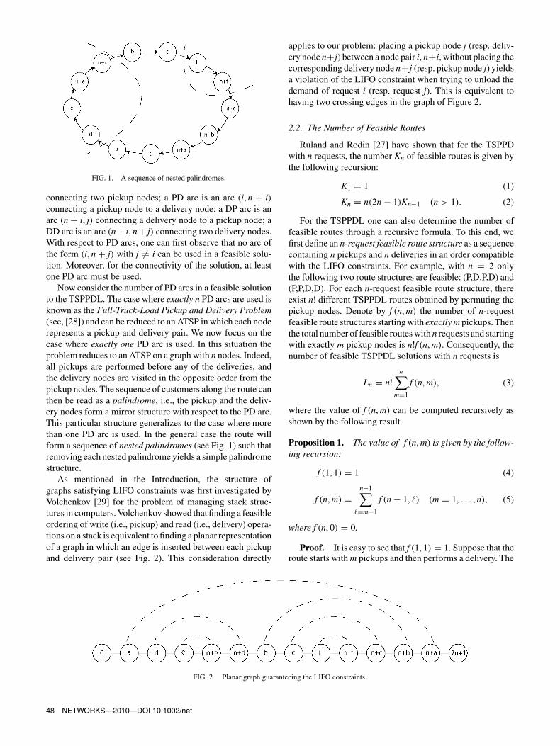
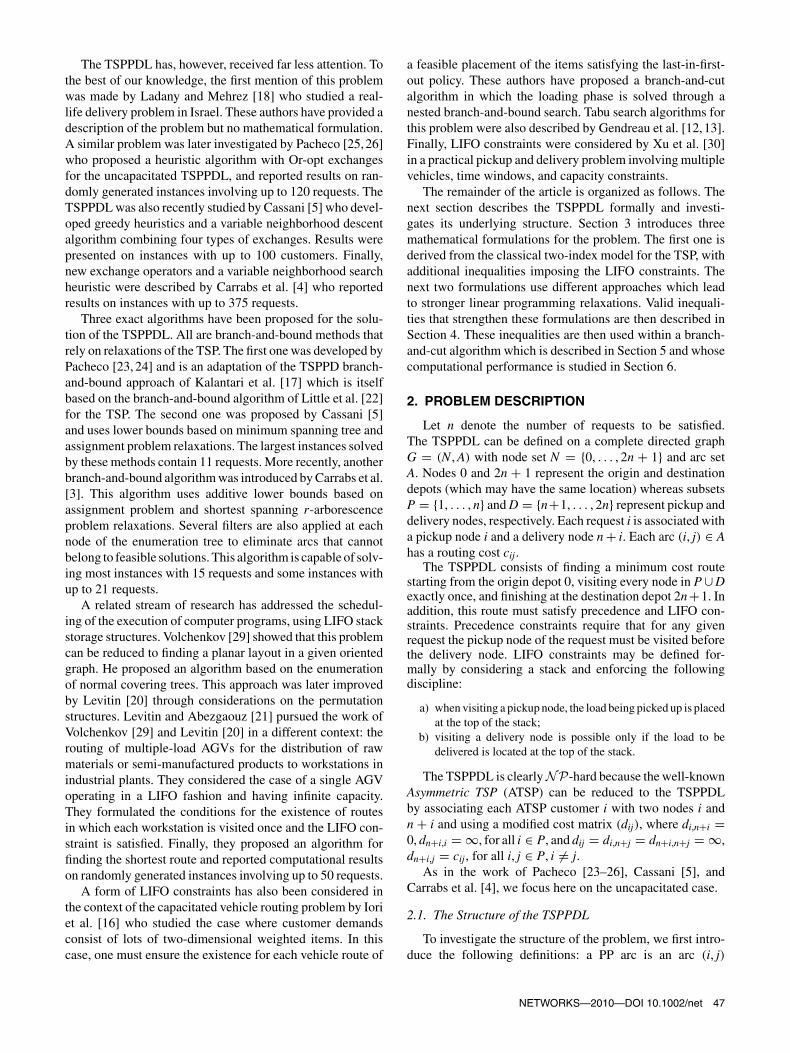
FIG. 1. A sequence of nested palindromes.

connecting two pickup nodes; a PD arc is an arc (i, n + i)connecting a pickup node to a delivery node; a DP arc is anarc (n + i, j) connecting a delivery node to a pickup node; aDD arc is an arc (n + i, n + j) connecting two delivery nodes.With respect to PD arcs, one can first observe that no arc ofthe form (i, n + j) with j �= i can be used in a feasible solu-tion. Moreover, for the connectivity of the solution, at leastone PD arc must be used.

Now consider the number of PD arcs in a feasible solutionto the TSPPDL. The case where exactly n PD arcs are used isknown as the Full-Truck-Load Pickup and Delivery Problem(see, [28]) and can be reduced to an ATSP in which each noderepresents a pickup and delivery pair. We now focus on thecase where exactly one PD arc is used. In this situation theproblem reduces to an ATSP on a graph with n nodes. Indeed,all pickups are performed before any of the deliveries, andthe delivery nodes are visited in the opposite order from thepickup nodes. The sequence of customers along the route canthen be read as a palindrome, i.e., the pickup and the deliv-ery nodes form a mirror structure with respect to the PD arc.This particular structure generalizes to the case where morethan one PD arc is used. In the general case the route willform a sequence of nested palindromes (see Fig. 1) such thatremoving each nested palindrome yields a simple palindromestructure.

As mentioned in the Introduction, the structure ofgraphs satisfying LIFO constraints was first investigated byVolchenkov [29] for the problem of managing stack struc-tures in computers. Volchenkov showed that finding a feasibleordering of write (i.e., pickup) and read (i.e., delivery) opera-tions on a stack is equivalent to finding a planar representationof a graph in which an edge is inserted between each pickupand delivery pair (see Fig. 2). This consideration directly

applies to our problem: placing a pickup node j (resp. deliv-ery node n+j) between a node pair i, n+i, without placing thecorresponding delivery node n+j (resp. pickup node j) yieldsa violation of the LIFO constraint when trying to unload thedemand of request i (resp. request j). This is equivalent tohaving two crossing edges in the graph of Figure 2.

2.2. The Number of Feasible Routes

Ruland and Rodin [27] have shown that for the TSPPDwith n requests, the number Kn of feasible routes is given bythe following recursion:

K1 = 1 (1)

Kn = n(2n − 1)Kn−1 (n > 1). (2)

For the TSPPDL one can also determine the number offeasible routes through a recursive formula. To this end, wefirst define an n-request feasible route structure as a sequencecontaining n pickups and n deliveries in an order compatiblewith the LIFO constraints. For example, with n = 2 onlythe following two route structures are feasible: (P,D,P,D) and(P,P,D,D). For each n-request feasible route structure, thereexist n! different TSPPDL routes obtained by permuting thepickup nodes. Denote by f (n, m) the number of n-requestfeasible route structures starting with exactly m pickups. Thenthe total number of feasible routes with n requests and startingwith exactly m pickup nodes is n!f (n, m). Consequently, thenumber of feasible TSPPDL solutions with n requests is

Ln = n!n∑

m=1

f (n, m), (3)

where the value of f (n, m) can be computed recursively asshown by the following result.

Proposition 1. The value of f (n, m) is given by the follow-ing recursion:

f (1, 1) = 1 (4)

f (n, m) =n−1∑

�=m−1

f (n − 1, �) (m = 1, . . . , n), (5)

where f (n, 0) = 0.

Proof. It is easy to see that f (1, 1) = 1. Suppose that theroute starts with m pickups and then performs a delivery. The

FIG. 2. Planar graph guaranteeing the LIFO constraints.

48 NETWORKS—2010—DOI 10.1002/net

TABLE 1. The number of feasible solutions with n requests.

n ATSP TSPPD TSPPDL

1 2 1 12 24 6 43 720 90 304 40,320 2,520 3365 3,628,800 113,400 5,0406 479,001,600 7,484,400 95,0407 87,178,291,200 681,080,400 2,162,1608 20,922,789,888,000 81,729,648,000 57,657,600

request just completed can be removed from further consid-eration. The vehicle then contains the first m −1 pickups andthere are two possible ways to extend the route:

a) Perform a delivery: the number of ways to extend the route inthis way is f (n − 1, m − 1) because m − 1 pickups have beenperformed and the corresponding deliveries have not yet beenperformed.

b) Perform one or more pickups. The number of ways to extendthe route in this way is

∑n−1�=m f (n − 1, �).

Hence

f (n, m) = f (n−1, m−1)+n−1∑�=m

f (n−1, �) =n−1∑

�=m−1

f (n−1, �).

■

Table 1 reports the number of feasible ATSP, TSPPD, andTSPPDL solutions for different values of n. For the ATSP, weindicate the number of feasible solutions in an instance with2n + 1 nodes (including the depot). Carrabs et al. [3] haveproposed a different (but equivalent) recursion for computingthe number of feasible routes in the TSPPDL.

3. MATHEMATICAL FORMULATIONS

In this section we first recall a classical formulation forthe TSPPD. We then introduce three different formulationsfor the (uncapacitated) TSPPDL.

To formulate the TSPPD, we associate to each arc (i, j) ∈A a binary variable xij taking value 1 if and only if nodej is visited immediately after node i. As usual, we defineS̄ = N \ S, x(S) = ∑

i,j∈S xij, x(δ+(S)) = ∑i∈S,j �∈S xij

and x(δ−(S)) = ∑i �∈S,j∈S xij. For any node i ∈ N , let

also x(i, S) = ∑j∈S xij and x(S, i) = ∑

j∈S xji. We alsodefine the collection S of all node subsets S ⊂ N such that0 ∈ S, 2n + 1 �∈ S and there exists a node i such that i �∈ Sand n + i ∈ S.

Using this notation, the TSPPD can then be formulated asthe following integer program:

(TSPPD) Minimize∑

(i,j)∈A

cijxij (6)

subject to

x(δ+(i)) = 1 ∀i ∈ P ∪ D ∪ {0} (7)

x(δ−(i)) = 1 ∀i ∈ P ∪ D ∪ {2n + 1} (8)

x(S) ≤ |S| − 1 ∀S ⊆ P ∪ D, |S| ≥ 2 (9)

x(S) ≤ |S| − 2 ∀S ∈ S (10)

xij ∈ {0, 1} ∀(i, j) ∈ A. (11)

The objective function (6) minimizes the total routing cost.Constraints (7) and (8) ensure that each pickup and deliv-ery node is visited exactly once. Constraints (9) ensure theconnectivity of the solution whereas constraints (10) imposethe precedence relationships between pickups and deliver-ies. Precedence constraints (10) were introduced by Balaset al. [2] in the context of the TSP with precedence con-straints, and by Ruland and Rodin [27] in the context of theTSPPD. Since the TSPPDL is a restriction of the TSPPD,these constraints are also valid for the former problem.

The TSPPDL can be formulated by introducing additionalsets of constraints in model (6)–(11). We now describe threesuch sets of constraints, giving rise to as many different for-mulations. The first two formulations require a polynomialnumber of additional variables and constraints whereas thethird one requires an exponential number of constraints butno new variable.

To describe the first and second formulations (which canhandle both the capacitated and uncapacitated versions ofthe problem), we associate each node i ∈ N with a demandparameter qi �= 0, such that qi = −qn+i for i = 1, . . . , n.The demand qi is positive for every pickup node i and isequal to −qi for the corresponding delivery node n + i. If theproblem is uncapacitated, one may simply set qi = 1, ∀i ∈ Pand qi = −1, ∀i ∈ D. We assume q0 = q2n+1 = 0. Toeach node i ∈ N , we also associate a continuous variableQi representing the load of the vehicle upon its departurefrom node i. Finally, we denote the vehicle capacity by Q.Again, if the TSPPDL is uncapacitated, one may simply setQ = n. Given this notation, LIFO constraints may be imposedthrough the following sets of constraints:

Qj ≥ (Qi + qj)xij ∀(i, j) ∈ A (12)

Qn+i = Qi − qi ∀i ∈ P (13)

max{0, qi} ≤ Qi ≤ min{Q, Q + qi} ∀i ∈ N . (14)

We denote model (6)–(14) by (TSPPDL1). The consis-tency of the load variables Qi is ensured through constraints(12), whereas constraints (13) enforce the LIFO policy.Finally, vehicle capacity is imposed through constraints (14).The following result demonstrates that constraints (7)–(14)properly define the LIFO policy.

Proposition 2. Constraints (10)–(13) are satisfied if andonly if the loading and unloading operations satisfy the LIFOpolicy.


Proof. Consider first a solution in which loading andunloading satisfy the LIFO constraints. It is clear that in sucha solution, the load of the vehicle immediately after visitingnode n + i is equal to Qi − qi. Indeed, if a pickup node jis visited between nodes i and n + i, then the correspondingdelivery node must also be visited, and vice-versa. As a result,the load of the vehicle upon arrival at node n + i is equal toits load upon departure from node i and hence (13).

Now consider a solution satisfying constraints (12)–(14).In this case, the net amount delivered between each pair i, n+iis equal to 0. Suppose that this solution does not satisfy theLIFO constraints. Then, one can find a node pair i, n + i suchthat at least one pickup node j is visited between i and n+i butnot the delivery node n + j. Let i′, n + i′ denote the first nodepair for which this condition is satisfied in the solution and letP̃ ⊂ P represent the set of pickup nodes for which the deliverynode is not visited between i′ and n + i′. Define q(P̃) =∑

j∈P̃ qj. Because the precedence constraints are satisfied,one cannot find a delivery node n + j between i′ and n + i′ ifthe corresponding pickup node j is not also visited between i′and n + i′. As a result, it follows that Qn+i = Qi − qi + q(P̃),a contradiction because q(P̃) > 0 and constraints (13) areassumed to hold. ■

Formulation (6)–(14) is nonlinear because of constraints(12). However, these constraints can be linearized as follows:

Qj ≥ Qi + qj − Wj(1 − xij) ∀i ∈ N , j ∈ N , (15)

where Wj = min{Q, Q + qj}. Moreover, Desrochers andLaporte [9] have shown that the inequalities (15) can be liftedby considering the reverse arc and imposing

Qj ≥ Qi + qj − Wj(1 − xij) + (Wj − qi − qj)xji ∀(i, j) ∈ A.(16)

Nevertheless, this formulation is likely to be weak becauseof the introduction of the Wj constants which typically leadto poor linear programming relaxation lower bounds.

A different formulation can be obtained by dropping the Qi

variables and associating with each arc (i, j) ∈ A a continuousvariable fij representing the load of the vehicle on that arc.Then, constraints (12)–(14) are replaced with the followingsets of linear constraints:

∑j∈N

fij −∑j∈N

fji = qi ∀i ∈ P ∪ D (17)

∑j∈N

fji −∑j∈N

fn+i,j = 0 ∀i ∈ P (18)

max{0, qi, −qj}xij ≤ fij ≤ min{Q, Q + qi, Q − qj}xij

∀(i, j) ∈ A. (19)

We denote the resulting formulation, (6)–(11) and (17)–(19), by (TSPPDL2). It is in fact inspired from the one-commodity flow formulation for the vehicle routing probleminitially proposed by Gavish and Graves [11].

Formulations (TSPPDL1) and (TSPPDL2) both requirethe introduction of additional variables in model (6)–(11).

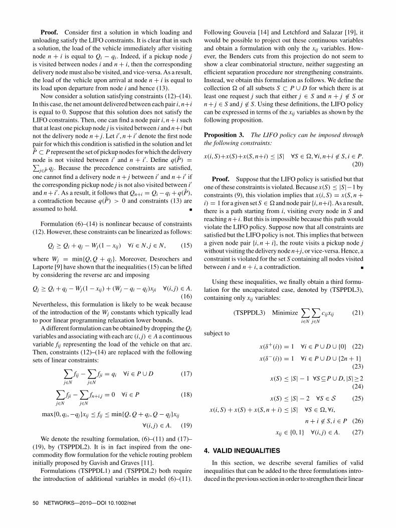
Following Gouveia [14] and Letchford and Salazar [19], itwould be possible to project out these continuous variablesand obtain a formulation with only the xij variables. How-ever, the Benders cuts from this projection do not seem toshow a clear combinatorial structure, neither suggesting anefficient separation procedure nor strengthening constraints.Instead, we obtain this formulation as follows. We define thecollection � of all subsets S ⊂ P ∪ D for which there is atleast one request j such that either j ∈ S and n + j �∈ S orn + j ∈ S and j �∈ S. Using these definitions, the LIFO policycan be expressed in terms of the xij variables as shown by thefollowing proposition.

Proposition 3. The LIFO policy can be imposed throughthe following constraints:

x(i, S)+x(S)+x(S, n+i) ≤ |S| ∀S ∈ �, ∀i, n+i �∈ S, i ∈ P.(20)

Proof. Suppose that the LIFO policy is satisfied but thatone of these constraints is violated. Because x(S) ≤ |S|−1 byconstraints (9), this violation implies that x(i, S) = x(S, n +i) = 1 for a given set S ∈ � and node pair {i, n+i}. As a result,there is a path starting from i, visiting every node in S andreaching n+ i. But this is impossible because this path wouldviolate the LIFO policy. Suppose now that all constraints aresatisfied but the LIFO policy is not. This implies that betweena given node pair {i, n + i}, the route visits a pickup node jwithout visiting the delivery node n+j, or vice-versa. Hence, aconstraint is violated for the set S containing all nodes visitedbetween i and n + i, a contradiction. ■

Using these inequalities, we finally obtain a third formu-lation for the uncapacitated case, denoted by (TSPPDL3),containing only xij variables:

(TSPPDL3) Minimize∑i∈N

∑j∈N

cijxij (21)

subject to

x(δ+(i)) = 1 ∀i ∈ P ∪ D ∪ {0} (22)

x(δ−(i)) = 1 ∀i ∈ P ∪ D ∪ {2n + 1}(23)

x(S) ≤ |S| − 1 ∀S ⊆P ∪ D, |S|≥2(24)

x(S) ≤ |S| − 2 ∀S ∈ S (25)

x(i, S) + x(S) + x(S, n + i) ≤ |S| ∀S ∈ �, ∀i,

n + i �∈ S, i ∈ P (26)

xij ∈ {0, 1} ∀(i, j) ∈ A. (27)

4. VALID INEQUALITIES

In this section, we describe several families of validinequalities that can be added to the three formulations intro-duced in the previous section in order to strengthen their linear


programming relaxation. We first describe known inequali-ties for the TSPPD and we then introduce new inequalitiesthat rely on the particular structure of the TSPPDL.

4.1. Known Inequalities for the TSPPD

Because the TSPPDL is a restriction of the TSPPD,valid inequalities for the latter problem are also valid forthe former. We now describe three known families of validinequalities for the TSPPD: strengthened subtour eliminationconstraints, strengthned cycle inequalities, and generalizedorder constraints.

The subtour elimination constraints (9) can be lifted in dif-ferent ways by considering the precedence relations betweenpickup i and delivery n + j. Let π(S) = {i ∈ P|n + i ∈ S}and σ(S) = {n + i ∈ D|i ∈ S} denote the sets of predeces-sors and successors of a given subset S ⊆ P∪D, respectively.Balas et al. [2] have introduced the following predecessor andsuccessor inequalities for the precedence-constrained ATSP:

x(S) +∑i∈S

∑

j∈S̄∩π(S)

xij +∑

i∈S∩π(S)

∑

j∈S̄\π(S)

xij ≤ |S| − 1,

(28)

x(S) +∑

i∈S̄∩σ(S)

∑j∈S

xij +∑

i∈S̄\σ(S)

∑j∈S∩σ(S)

xij ≤ |S| − 1.

(29)

Cycle inequalities for the ATSP can be strengthened asexplained by Grötschel and Padberg [15]. For a given orderedset S = {i1, i2, . . . , ik} ⊆ N , with k ≥ 3, they proposed twofamilies of valid inequalities, called D+

k and D−k inequalities:

k−1∑h=1

xih,ih+1 + xik ,i1 + 2k−1∑h=2

xih,i1 +k−1∑h=3

h−1∑l=2

xih,il ≤ k − 1,

(30)

k−1∑h=1

xih,ih+1 + xik ,i1 + 2k∑

h=3

xi1,ih +k∑

h=4

h−1∑l=3

xih,il ≤ k − 1.

(31)

Cordeau [6] has shown that because of precedence con-straints the latter inequalities can be strengthened by consid-ering the sets π(S) and σ(S) as in inequalities (28) and (29),leading to:

k−1∑h=1

xih,ih+1 + xik ,i1 + 2k−1∑h=2

xih,i1 +k−1∑h=3

h−1∑l=2

xih,il

+∑

n+ip∈S̄∩σ(S)

xn+ip,i1 ≤ k − 1, (32)

k−1∑h=1

xih,ih+1 + xik ,i1 + 2k∑

h=3

xi1,ih +k∑

h=4

h−1∑l=3

xih,il

+∑

ip∈S̄∩π(S)

xi1,ip ≤ k − 1. (33)

Finally, let U1, . . . , Uk ⊂ P ∪ D be mutually disjointsubsets such that i1, . . . , ik ∈ P are requests for whichil, n + il+1 ∈ Ul for l = 1, . . . , k (where ik+1 = i1). Thefollowing precedence cycle breaking inequalities were intro-duced by Balas et al. [2] for the precedence-constrainedTSP:

k∑l=1

x(Ul) ≤k∑

l=1

|Ul| − k − 1. (34)

Equivalent inequalities, called generalized order con-straints were introduced by Ruland and Rodin [27] for theundirected TSPPD.

Several other families of valid inequalities for the TSPPDhave been described by Ruland and Rodin [27] and byDumitrescu et al. [10]. However, our experiments have shownthat they have a negligible impact in a branch-and-cut algo-rithm for the TSPPDL. In the next section we thus introducenew inequalities that take advantage of the particular structureof the problem.

4.2. New Inequalities for the TSPPDL

We now describe three new families of inequalities for theTSPPDL. Throughout this section, we denote by i ≺ j thefact that node i is a predecessor of node j in a route.

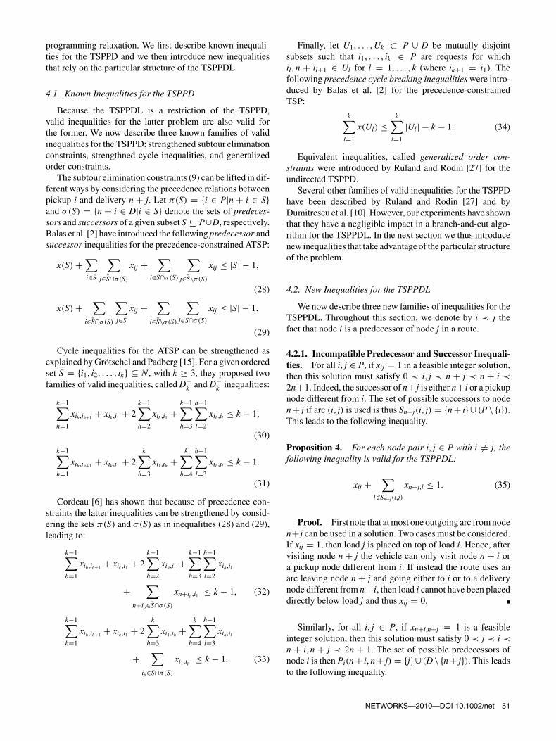
4.2.1. Incompatible Predecessor and Successor Inequali-ties. For all i, j ∈ P, if xij = 1 in a feasible integer solution,then this solution must satisfy 0 ≺ i, j ≺ n + j ≺ n + i ≺2n+1. Indeed, the successor of n+j is either n+i or a pickupnode different from i. The set of possible successors to noden + j if arc (i, j) is used is thus Sn+j(i, j) = {n + i} ∪ (P \ {i}).This leads to the following inequality.

Proposition 4. For each node pair i, j ∈ P with i �= j, thefollowing inequality is valid for the TSPPDL:

xij +∑

l �∈Sn+j(i,j)

xn+j,l ≤ 1. (35)

Proof. First note that at most one outgoing arc from noden+ j can be used in a solution. Two cases must be considered.If xij = 1, then load j is placed on top of load i. Hence, aftervisiting node n + j the vehicle can only visit node n + i ora pickup node different from i. If instead the route uses anarc leaving node n + j and going either to i or to a deliverynode different from n+ i, then load i cannot have been placeddirectly below load j and thus xij = 0. ■

Similarly, for all i, j ∈ P, if xn+i,n+j = 1 is a feasibleinteger solution, then this solution must satisfy 0 ≺ j ≺ i ≺n + i, n + j ≺ 2n + 1. The set of possible predecessors ofnode i is then Pi(n + i, n + j) = {j}∪ (D \ {n + j}). This leadsto the following inequality.


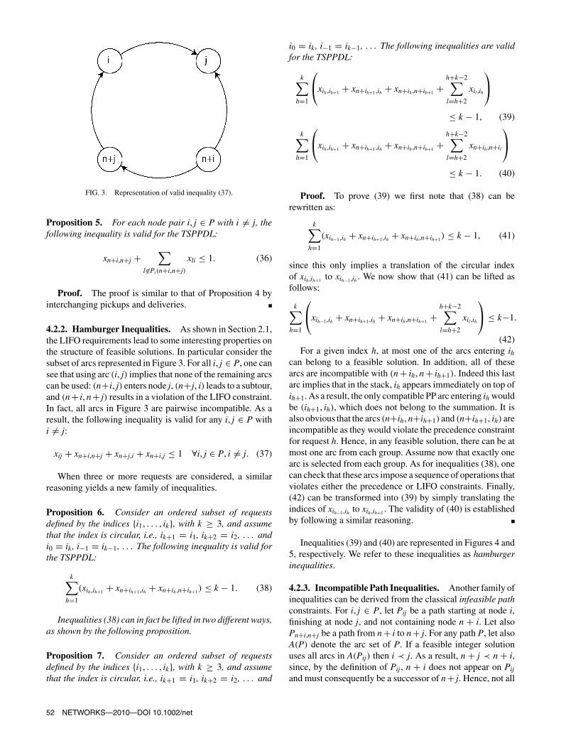
FIG. 3. Representation of valid inequality (37).

Proposition 5. For each node pair i, j ∈ P with i �= j, thefollowing inequality is valid for the TSPPDL:

xn+i,n+j +∑

l �∈Pi(n+i,n+j)

xli ≤ 1. (36)

Proof. The proof is similar to that of Proposition 4 byinterchanging pickups and deliveries. ■

4.2.2. Hamburger Inequalities. As shown in Section 2.1,the LIFO requirements lead to some interesting properties onthe structure of feasible solutions. In particular consider thesubset of arcs represented in Figure 3. For all i, j ∈ P, one cansee that using arc (i, j) implies that none of the remaining arcscan be used: (n+i, j) enters node j, (n+j, i) leads to a subtour,and (n+ i, n+ j) results in a violation of the LIFO constraint.In fact, all arcs in Figure 3 are pairwise incompatible. As aresult, the following inequality is valid for any i, j ∈ P withi �= j:

xij + xn+i,n+j + xn+j,i + xn+i,j ≤ 1 ∀i, j ∈ P, i �= j. (37)

When three or more requests are considered, a similarreasoning yields a new family of inequalities.

Proposition 6. Consider an ordered subset of requestsdefined by the indices {i1, . . . , ik}, with k ≥ 3, and assumethat the index is circular, i.e., ik+1 = i1, ik+2 = i2, . . . andi0 = ik , i−1 = ik−1, . . . The following inequality is valid forthe TSPPDL:

k∑h=1

(xih,ih+1 + xn+ih+1,ih + xn+ih,n+ih+1) ≤ k − 1. (38)

Inequalities (38) can in fact be lifted in two different ways,as shown by the following proposition.

Proposition 7. Consider an ordered subset of requestsdefined by the indices {i1, . . . , ik}, with k ≥ 3, and assumethat the index is circular, i.e., ik+1 = i1, ik+2 = i2, . . . and

i0 = ik , i−1 = ik−1, . . . The following inequalities are validfor the TSPPDL:

k∑h=1

xih,ih+1 + xn+ih+1,ih + xn+ih,n+ih+1 +

h+k−2∑l=h+2

xil ,ih

≤ k − 1, (39)

k∑h=1

xih,ih+1 + xn+ih+1,ih + xn+ih,n+ih+1 +

h+k−2∑l=h+2

xn+ih,n+il

≤ k − 1. (40)

Proof. To prove (39) we first note that (38) can berewritten as:

k∑h=1

(xih−1,ih + xn+ih+1,ih + xn+ih,n+ih+1) ≤ k − 1, (41)

since this only implies a translation of the circular indexof xih,ih+1 to xih−1,ih . We now show that (41) can be lifted asfollows:

k∑h=1

xih−1,ih + xn+ih+1,ih + xn+ih,n+ih+1 +

h+k−2∑l=h+2

xil ,ih

≤ k−1.

(42)For a given index h, at most one of the arcs entering ih

can belong to a feasible solution. In addition, all of thesearcs are incompatible with (n + ih, n + ih+1). Indeed this lastarc implies that in the stack, ih appears immediately on top ofih+1. As a result, the only compatible PP arc entering ih wouldbe (ih+1, ih), which does not belong to the summation. It isalso obvious that the arcs (n+ih, n+ih+1) and (n+ih+1, ih) areincompatible as they would violate the precedence constraintfor request h. Hence, in any feasible solution, there can be atmost one arc from each group. Assume now that exactly onearc is selected from each group. As for inequalities (38), onecan check that these arcs impose a sequence of operations thatviolates either the precedence or LIFO constraints. Finally,(42) can be transformed into (39) by simply translating theindices of xih−1,ih to xih,ih+1 . The validity of (40) is establishedby following a similar reasoning. ■

Inequalities (39) and (40) are represented in Figures 4 and5, respectively. We refer to these inequalities as hamburgerinequalities.

4.2.3. Incompatible Path Inequalities. Another family ofinequalities can be derived from the classical infeasible pathconstraints. For i, j ∈ P, let Pij be a path starting at node i,finishing at node j, and not containing node n + i. Let alsoPn+i,n+j be a path from n + i to n + j. For any path P, let alsoA(P) denote the arc set of P. If a feasible integer solutionuses all arcs in A(Pij) then i ≺ j. As a result, n + j ≺ n + i,since, by the definition of Pij, n + i does not appear on Pij

and must consequently be a successor of n+ j. Hence, not all


FIG. 4. Hamburger inequality (39) with four requests.

arcs in A(Pn+i,n+j) can be used. This observation proves thefollowing proposition.

Proposition 8. Consider two requests i, j ∈ P. For any pathPij = (k1, . . . , kp) with k1 = i, kp = j and kh �= n+i, 2 ≤ h ≤p−1, and any path Pn+i,n+j = (l1, . . . , lq) with l1 = n+i andlq = n + j, the following inequality is valid for the TSPPDL:

p−1∑h=1

xkh,kh+1 +q−1∑h=1

xlh,lh+1 ≤ |A(Pij)|+|A(Pn+i,n+j)|−1. (43)

These inequalities can in fact be lifted by following thestrengthening of infeasible path constraints into tournamentinequalities introduced by Ascheuer et al. [1]. This idea leadsto the following form:

p−1∑h=1

p∑r=h+1

xkh,kr +q−1∑h=1

q∑r=h+1

xlh,lr ≤ |A(Pij)|+|A(Pn+i,n+j)|−1.

(44)

5. BRANCH-AND-CUT ALGORITHM

The formulations presented in Section 3 and the validinequalities introduced in Section 4 are used within a branch-and-cut algorithm which we now describe in detail.

5.1. Preprocessing and Cut Pool

As noted earlier, no delivery node n + j can be the directsuccessor of a pick-up node i when j �= i. As a result, arcs ofthe form (i, n + j) with i �= j can be removed from the graph.

Before starting the algorithm, we add the following setof inequalities to the models. Because there is a quadraticnumber of inequalities (35) and (36), these are all introduced

into the cut pool. Similarly, we include all subtour eliminationconstraints (9) with |S| = 2 as well as all constraints (37)whose number is also quadratic. We also add to the modelthe simple predecessor and successor inequalities, obtainedby setting S equal to {i, j}, {i, n + j} and {i, n + i, j} in (28),and to {n + i, n + j}, {i, n + j} and {i, n + i, n + j} in (29).Finally, we include simple cases of the strengthened D+

h andD−

h inequalities: xn+i,j +xji+xi,n+i+xn+j,n+i ≤ 2 and xi,n+i+xn+i,n+j + xn+j,i + xi,j ≤ 2.

5.2. Separation Procedures

In our branch-and-cut algorithm, we use exact separationprocedures for subtour elimination constraints (9), prece-dence constraints (10), and LIFO constraints (26). The firsttwo groups of constraints are required to ensure feasibilityin all three formulations, whereas the third group of con-straints is necessary for formulation (TSPPDL3). For theseparation of inequalities (28)–(29), (32)–(34), (39), (40),and (43), however, we use heuristics.

5.2.1. Exact Separation Procedures. Constraints (9) areseparated exactly in the classical way. Given a (fractional)solution x∗, we create a supporting graph G∗ = (N , A∗),where an arc (i, j) ∈ A∗ has capacity equal to x∗

ij. We thensolve a max-flow problem on G∗, from 0 to each pickup i,and from each delivery n + i to 2n + 1 (i = 1, . . . , n).

Constraints (10) are separated exactly for each i ∈ P inthe following way:

1. create the supporting graph G∗;2. connect 0 to n + i and i to 2n + 1 (i = 1, . . . , n) with arcs of

capacity 2;3. solve the max-flow problem from 0 to 2n + 1 and obtain a

set S∗ containing 0 (note that by construction i �∈ S∗ andn + i ∈ S∗). If the max-flow value is smaller than 2, then S∗defines a violated inequality (10).

FIG. 5. Hamburger inequality (40) with four requests.


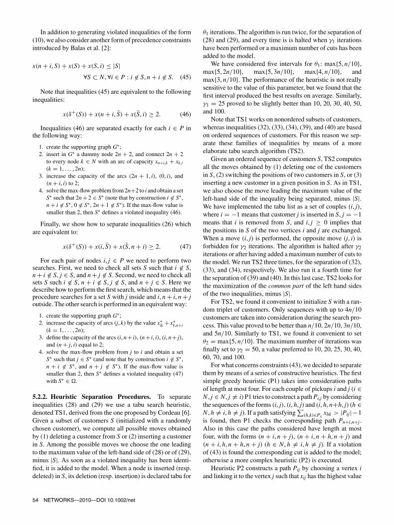
In addition to generating violated inequalities of the form(10), we also consider another form of precedence constraintsintroduced by Balas et al. [2]:

x(n + i, S) + x(S) + x(S, i) ≤ |S|∀S ⊂ N , ∀i ∈ P : i �∈ S, n + i �∈ S. (45)

Note that inequalities (45) are equivalent to the followinginequalities:

x(δ+(S)) + x(n + i, S̄) + x(S̄, i) ≥ 2. (46)

Inequalities (46) are separated exactly for each i ∈ P inthe following way:

1. create the supporting graph G∗;2. insert in G∗ a dummy node 2n + 2, and connect 2n + 2

to every node k ∈ N with an arc of capacity xn+i,k + xk,i

(k = 1, . . . , 2n);3. increase the capacity of the arcs (2n + 1, i), (0, i), and

(n + i, i) to 2;4. solve the max-flow problem from 2n+2 to i and obtain a set

S∗ such that 2n + 2 ∈ S∗ (note that by construction i �∈ S∗,n + i �∈ S∗, 0 �∈ S∗, 2n + 1 �∈ S∗). If the max-flow value issmaller than 2, then S∗ defines a violated inequality (46).

Finally, we show how to separate inequalities (26) whichare equivalent to:

x(δ+(S)) + x(i, S̄) + x(S̄, n + i) ≥ 2. (47)

For each pair of nodes i, j ∈ P we need to perform twosearches. First, we need to check all sets S such that i �∈ S,n + i �∈ S, j ∈ S, and n + j �∈ S. Second, we need to check allsets S such i �∈ S, n + i �∈ S, j �∈ S, and n + j ∈ S. Here wedescribe how to perform the first search, which means that theprocedure searches for a set S with j inside and i, n + i, n + joutside. The other search is performed in an equivalent way:

1. create the supporting graph G∗;2. increase the capacity of arcs (j, k) by the value x∗

ik + x∗k,n+i

(k = 1, . . . , 2n);3. define the capacity of the arcs (i, n+ i), (n+ i, i), (i, n+ j),

and (n + j, i) equal to 2;4. solve the max-flow problem from j to i and obtain a set

S∗ such that j ∈ S∗ (and note that by construction i �∈ S∗,n + i �∈ S∗, and n + j �∈ S∗). If the max-flow value issmaller than 2, then S∗ defines a violated inequality (47)with S∗ ∈ �.

5.2.2. Heuristic Separation Procedures. To separateinequalities (28) and (29) we use a tabu search heuristic,denoted TS1, derived from the one proposed by Cordeau [6].Given a subset of customers S (initialized with a randomlychosen customer), we compute all possible moves obtainedby (1) deleting a customer from S or (2) inserting a customerin S. Among the possible moves we choose the one leadingto the maximum value of the left-hand side of (28) or of (29),minus |S|. As soon as a violated inequality has been identi-fied, it is added to the model. When a node is inserted (resp.deleted) in S, its deletion (resp. insertion) is declared tabu for

θ1 iterations. The algorithm is run twice, for the separation of(28) and (29), and every time is is halted when γ1 iterationshave been performed or a maximum number of cuts has beenadded to the model.

We have considered five intervals for θ1: max{5, n/10},max{5, 2n/10}, max{5, 3n/10}, max{4, n/10}, andmax{3, n/10}. The performance of the heuristic is not reallysensitive to the value of this parameter, but we found that thefirst interval produced the best results on average. Similarly,γ1 = 25 proved to be slightly better than 10, 20, 30, 40, 50,and 100.

Note that TS1 works on nonordered subsets of customers,whereas inequalities (32), (33), (34), (39), and (40) are basedon ordered sequences of customers. For this reason we sep-arate these families of inequalities by means of a moreelaborate tabu search algorithm (TS2).

Given an ordered sequence of customers S, TS2 computesall the moves obtained by (1) deleting one of the customersin S, (2) switching the positions of two customers in S, or (3)inserting a new customer in a given position in S. As in TS1,we also choose the move leading the maximum value of theleft-hand side of the inequality being separated, minus |S|.We have implemented the tabu list as a set of couples (i, j),where i = −1 means that customer j is inserted in S, j = −1means that i is removed from S, and i, j ≥ 0 implies thatthe positions in S of the two vertices i and j are exchanged.When a move (i, j) is performed, the opposite move (j, i) isforbidden for γ2 iterations. The algorithm is halted after γ2

iterations or after having added a maximum number of cuts tothe model. We run TS2 three times, for the separation of (32),(33), and (34), respectively. We also run it a fourth time forthe separation of (39) and (40). In this last case, TS2 looks forthe maximization of the common part of the left hand sidesof the two inequalities, minus |S|.

For TS2, we found it convenient to initialize S with a ran-dom triplet of customers. Only sequences with up to 4n/10customers are taken into consideration during the search pro-cess. This value proved to be better than n/10, 2n/10, 3n/10,and 5n/10. Similarly to TS1, we found it convenient to setθ2 = max{5, n/10}. The maximum number of iterations wasfinally set to γ2 = 50, a value preferred to 10, 20, 25, 30, 40,60, 70, and 100.

For what concerns constraints (43), we decided to separatethem by means of a series of constructive heuristics. The firstsimple greedy heuristic (P1) takes into consideration pathsof length at most four. For each couple of pickups i and j (i ∈N , j ∈ N , j �= i) P1 tries to construct a path Pi,j by consideringthe sequences of the forms (i, j), (i, h, j) and (i, h, n+h, j) (h ∈N , h �= i, h �= j). If a path satisfying

∑(h,k)∈Pij

xhk > |Pij|−1is found, then P1 checks the corresponding path Pn+i,n+j.Also in this case the paths considered have length at mostfour, with the forms (n + i, n + j), (n + i, n + h, n + j) and(n + i, h, n + h, n + j) (h ∈ N , h �= i, h �= j). If a violationof (43) is found the corresponding cut is added to the model;otherwise a more complex heuristic (P2) is executed.

Heuristic P2 constructs a path Pij by choosing a vertex iand linking it to the vertex j such that xij has the highest value


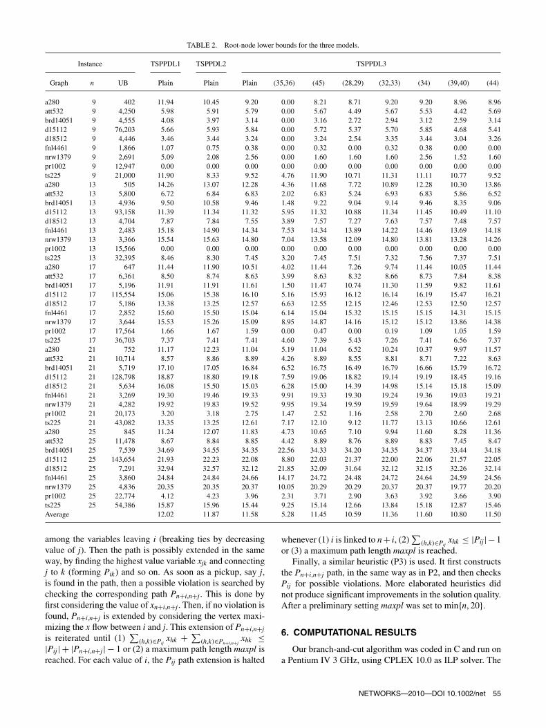
TABLE 2. Root-node lower bounds for the three models.

Instance TSPPDL1 TSPPDL2 TSPPDL3

Graph n UB Plain Plain Plain (35,36) (45) (28,29) (32,33) (34) (39,40) (44)

a280 9 402 11.94 10.45 9.20 0.00 8.21 8.71 9.20 9.20 8.96 8.96att532 9 4,250 5.98 5.91 5.79 0.00 5.67 4.49 5.67 5.53 4.42 5.69brd14051 9 4,555 4.08 3.97 3.14 0.00 3.16 2.72 2.94 3.12 2.59 3.14d15112 9 76,203 5.66 5.93 5.84 0.00 5.72 5.37 5.70 5.85 4.68 5.41d18512 9 4,446 3.46 3.44 3.24 0.00 3.24 2.54 3.35 3.44 3.04 3.26fnl4461 9 1,866 1.07 0.75 0.38 0.00 0.32 0.00 0.32 0.38 0.00 0.00nrw1379 9 2,691 5.09 2.08 2.56 0.00 1.60 1.60 1.60 2.56 1.52 1.60pr1002 9 12,947 0.00 0.00 0.00 0.00 0.00 0.00 0.00 0.00 0.00 0.00ts225 9 21,000 11.90 8.33 9.52 4.76 11.90 10.71 11.31 11.11 10.77 9.52a280 13 505 14.26 13.07 12.28 4.36 11.68 7.72 10.89 12.28 10.30 13.86att532 13 5,800 6.72 6.84 6.83 2.02 6.83 5.24 6.93 6.83 5.86 6.52brd14051 13 4,936 9.50 10.58 9.46 1.48 9.22 9.04 9.14 9.46 8.35 9.06d15112 13 93,158 11.39 11.34 11.32 5.95 11.32 10.88 11.34 11.45 10.49 11.10d18512 13 4,704 7.87 7.84 7.55 3.89 7.57 7.27 7.63 7.57 7.48 7.57fnl4461 13 2,483 15.18 14.90 14.34 7.53 14.34 13.89 14.22 14.46 13.69 14.18nrw1379 13 3,366 15.54 15.63 14.80 7.04 13.58 12.09 14.80 13.81 13.28 14.26pr1002 13 15,566 0.00 0.00 0.00 0.00 0.00 0.00 0.00 0.00 0.00 0.00ts225 13 32,395 8.46 8.30 7.45 3.20 7.45 7.51 7.32 7.56 7.37 7.51a280 17 647 11.44 11.90 10.51 4.02 11.44 7.26 9.74 11.44 10.05 11.44att532 17 6,361 8.50 8.74 8.63 3.99 8.63 8.32 8.66 8.73 7.84 8.38brd14051 17 5,196 11.91 11.91 11.61 1.50 11.47 10.74 11.30 11.59 9.82 11.61d15112 17 115,554 15.06 15.38 16.10 5.16 15.93 16.12 16.14 16.19 15.47 16.21d18512 17 5,186 13.38 13.25 12.57 6.63 12.55 12.15 12.46 12.53 12.50 12.57fnl4461 17 2,852 15.60 15.50 15.04 6.14 15.04 15.32 15.15 15.15 14.31 15.15nrw1379 17 3,644 15.53 15.26 15.09 8.95 14.87 14.16 15.12 15.12 13.86 14.38pr1002 17 17,564 1.66 1.67 1.59 0.00 0.47 0.00 0.19 1.09 1.05 1.59ts225 17 36,703 7.37 7.41 7.41 4.60 7.39 5.43 7.26 7.41 6.56 7.37a280 21 752 11.17 12.23 11.04 5.19 11.04 6.52 10.24 10.37 9.97 11.57att532 21 10,714 8.57 8.86 8.89 4.26 8.89 8.55 8.81 8.71 7.22 8.63brd14051 21 5,719 17.10 17.05 16.84 6.52 16.75 16.49 16.79 16.66 15.79 16.72d15112 21 128,798 18.87 18.80 19.18 7.59 19.06 18.82 19.14 19.19 18.45 19.16d18512 21 5,634 16.08 15.50 15.03 6.28 15.00 14.39 14.98 15.14 15.18 15.09fnl4461 21 3,269 19.30 19.46 19.33 9.91 19.33 19.30 19.24 19.36 19.03 19.21nrw1379 21 4,282 19.92 19.83 19.52 9.95 19.34 19.59 19.59 19.64 18.99 19.29pr1002 21 20,173 3.20 3.18 2.75 1.47 2.52 1.16 2.58 2.70 2.60 2.68ts225 21 43,082 13.35 13.25 12.61 7.17 12.10 9.12 11.77 13.13 10.66 12.61a280 25 845 11.24 12.07 11.83 4.73 10.65 7.10 9.94 11.60 8.28 11.36att532 25 11,478 8.67 8.84 8.85 4.42 8.89 8.76 8.89 8.83 7.45 8.47brd14051 25 7,539 34.69 34.55 34.35 22.56 34.33 34.20 34.35 34.37 33.44 34.18d15112 25 143,654 21.93 22.23 22.08 8.80 22.03 21.37 22.00 22.06 21.57 22.05d18512 25 7,291 32.94 32.57 32.12 21.85 32.09 31.64 32.12 32.15 32.26 32.14fnl4461 25 3,860 24.84 24.84 24.66 14.17 24.72 24.48 24.72 24.64 24.59 24.56nrw1379 25 4,836 20.35 20.35 20.37 10.05 20.29 20.29 20.37 20.37 19.77 20.20pr1002 25 22,774 4.12 4.23 3.96 2.31 3.71 2.90 3.63 3.92 3.66 3.90ts225 25 54,386 15.87 15.96 15.44 9.25 15.14 12.66 13.84 15.18 12.87 15.46Average 12.02 11.87 11.58 5.28 11.45 10.59 11.36 11.60 10.80 11.50

among the variables leaving i (breaking ties by decreasingvalue of j). Then the path is possibly extended in the sameway, by finding the highest value variable xjk and connectingj to k (forming Pik) and so on. As soon as a pickup, say j,is found in the path, then a possible violation is searched bychecking the corresponding path Pn+i,n+j. This is done byfirst considering the value of xn+i,n+j. Then, if no violation isfound, Pn+i,n+j is extended by considering the vertex maxi-mizing the x flow between i and j. This extension of Pn+i,n+j

is reiterated until (1)∑

(h,k)∈Pijxhk + ∑

(h,k)∈Pn+i,n+jxhk ≤

|Pij| + |Pn+i,n+j| − 1 or (2) a maximum path length maxpl isreached. For each value of i, the Pij path extension is halted

whenever (1) i is linked to n+ i, (2)∑

(h,k)∈Pijxhk ≤ |Pij|−1

or (3) a maximum path length maxpl is reached.Finally, a similar heuristic (P3) is used. It first constructs

the Pn+i,n+j path, in the same way as in P2, and then checksPij for possible violations. More elaborated heuristics didnot produce significant improvements in the solution quality.After a preliminary setting maxpl was set to min{n, 20}.

6. COMPUTATIONAL RESULTS

Our branch-and-cut algorithm was coded in C and run ona Pentium IV 3 GHz, using CPLEX 10.0 as ILP solver. The


tests were executed on the instances introduced by Carrabset al. [3], by considering up to 25 requests (52 nodes), leadingto a total of 45 instances.

To reduce the CPU time spent by the separation proce-dures, at each node of the branch-and-cut tree we stop lookingfor violated valid inequalities after 8 violated inequalitieshave been added to the model. This value was chosen experi-mentally by performing sensitivity analyses on our set of testinstances.

Table 2 presents the root-node lower bounds obtained forthe three models presented in the previous sections. Thenames of the original TSP instances used to produce validTSPPDL instances are given in column Graph. In column nwe give the number of requests and in column UB we reportthe best upper bound that we obtained for each instance.

Our algorithm takes as an initial upper bound the valueobtained by the VNS heuristic of Carrabs et al. [4]. Theseupper bounds are identical to the ones in Column UB,except for three cases where our algorithm could improve thesolution found by the heuristic. In particular, for instancesnrw1379 with n = 17, att532 with n = 25, and ts225with n = 25, we obtained solutions with cost 3644 (versus3652), 11478 (versus 11,484) and 54,386 (versus 54,629),respectively.

The values in the remaining columns are given as per-centage gaps between the lower bound obtained by a modeland UB, computed as 100(UB − LB)/UB. In particular, wereport the percentage gap obtained by each of the plainformulations TSPPDL1, TSPPDL2, and TSPPDL3. For TSP-PDL3 we also report the percentage gaps obtained by addingone family of inequalities at a time to the plain formula-tion (e.g., column (35,36) reports the value obtained withformulation TSPPDL3 plus constraints (35) and (36)). Thethree plain formulations present similar percentage gaps, withTSPPDL3 obtaining a slightly better average value (11.58%).This value is consistently improved by the quadratic familiesof inequalities (35) and (36) which together lead to a gap of5.28%. Smaller improvements are obtained by consideringthe other inequalities, with the generalized order constraints(34) being the least effective family, leading to no significantimprovement.

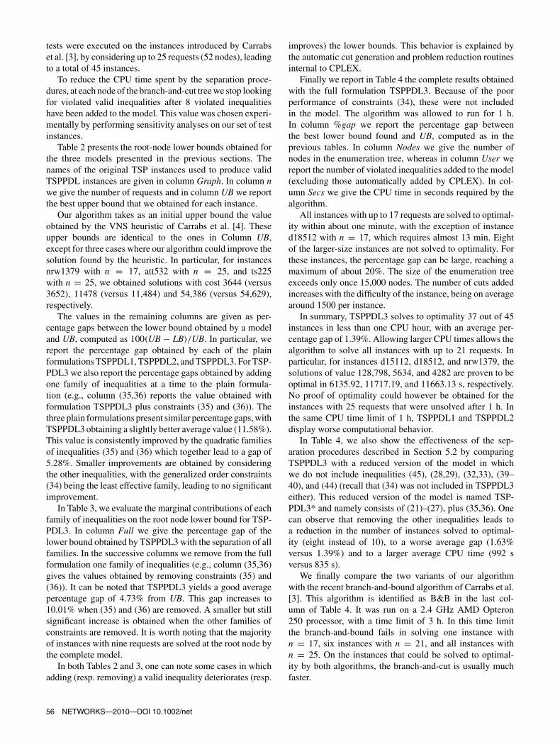
In Table 3, we evaluate the marginal contributions of eachfamily of inequalities on the root node lower bound for TSP-PDL3. In column Full we give the percentage gap of thelower bound obtained by TSPPDL3 with the separation of allfamilies. In the successive columns we remove from the fullformulation one family of inequalities (e.g., column (35,36)gives the values obtained by removing constraints (35) and(36)). It can be noted that TSPPDL3 yields a good averagepercentage gap of 4.73% from UB. This gap increases to10.01% when (35) and (36) are removed. A smaller but stillsignificant increase is obtained when the other families ofconstraints are removed. It is worth noting that the majorityof instances with nine requests are solved at the root node bythe complete model.

In both Tables 2 and 3, one can note some cases in whichadding (resp. removing) a valid inequality deteriorates (resp.

improves) the lower bounds. This behavior is explained bythe automatic cut generation and problem reduction routinesinternal to CPLEX.

Finally we report in Table 4 the complete results obtainedwith the full formulation TSPPDL3. Because of the poorperformance of constraints (34), these were not includedin the model. The algorithm was allowed to run for 1 h.In column %gap we report the percentage gap betweenthe best lower bound found and UB, computed as in theprevious tables. In column Nodes we give the number ofnodes in the enumeration tree, whereas in column User wereport the number of violated inequalities added to the model(excluding those automatically added by CPLEX). In col-umn Secs we give the CPU time in seconds required by thealgorithm.

All instances with up to 17 requests are solved to optimal-ity within about one minute, with the exception of instanced18512 with n = 17, which requires almost 13 min. Eightof the larger-size instances are not solved to optimality. Forthese instances, the percentage gap can be large, reaching amaximum of about 20%. The size of the enumeration treeexceeds only once 15,000 nodes. The number of cuts addedincreases with the difficulty of the instance, being on averagearound 1500 per instance.

In summary, TSPPDL3 solves to optimality 37 out of 45instances in less than one CPU hour, with an average per-centage gap of 1.39%. Allowing larger CPU times allows thealgorithm to solve all instances with up to 21 requests. Inparticular, for instances d15112, d18512, and nrw1379, thesolutions of value 128,798, 5634, and 4282 are proven to beoptimal in 6135.92, 11717.19, and 11663.13 s, respectively.No proof of optimality could however be obtained for theinstances with 25 requests that were unsolved after 1 h. Inthe same CPU time limit of 1 h, TSPPDL1 and TSPPDL2display worse computational behavior.

In Table 4, we also show the effectiveness of the sep-aration procedures described in Section 5.2 by comparingTSPPDL3 with a reduced version of the model in whichwe do not include inequalities (45), (28,29), (32,33), (39–40), and (44) (recall that (34) was not included in TSPPDL3either). This reduced version of the model is named TSP-PDL3* and namely consists of (21)–(27), plus (35,36). Onecan observe that removing the other inequalities leads toa reduction in the number of instances solved to optimal-ity (eight instead of 10), to a worse average gap (1.63%versus 1.39%) and to a larger average CPU time (992 sversus 835 s).

We finally compare the two variants of our algorithmwith the recent branch-and-bound algorithm of Carrabs et al.[3]. This algorithm is identified as B&B in the last col-umn of Table 4. It was run on a 2.4 GHz AMD Opteron250 processor, with a time limit of 3 h. In this time limitthe branch-and-bound fails in solving one instance withn = 17, six instances with n = 21, and all instances withn = 25. On the instances that could be solved to optimal-ity by both algorithms, the branch-and-cut is usually muchfaster.


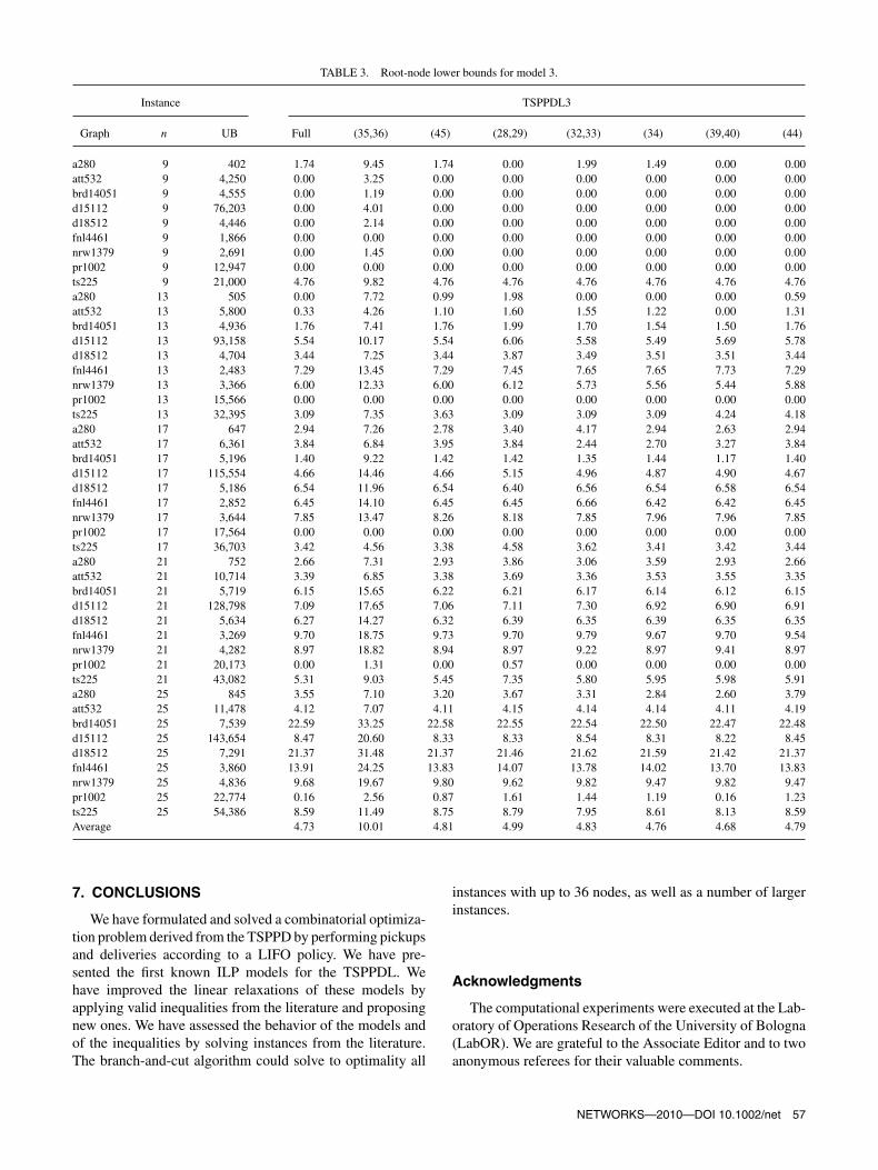
TABLE 3. Root-node lower bounds for model 3.

Instance TSPPDL3

Graph n UB Full (35,36) (45) (28,29) (32,33) (34) (39,40) (44)

a280 9 402 1.74 9.45 1.74 0.00 1.99 1.49 0.00 0.00att532 9 4,250 0.00 3.25 0.00 0.00 0.00 0.00 0.00 0.00brd14051 9 4,555 0.00 1.19 0.00 0.00 0.00 0.00 0.00 0.00d15112 9 76,203 0.00 4.01 0.00 0.00 0.00 0.00 0.00 0.00d18512 9 4,446 0.00 2.14 0.00 0.00 0.00 0.00 0.00 0.00fnl4461 9 1,866 0.00 0.00 0.00 0.00 0.00 0.00 0.00 0.00nrw1379 9 2,691 0.00 1.45 0.00 0.00 0.00 0.00 0.00 0.00pr1002 9 12,947 0.00 0.00 0.00 0.00 0.00 0.00 0.00 0.00ts225 9 21,000 4.76 9.82 4.76 4.76 4.76 4.76 4.76 4.76a280 13 505 0.00 7.72 0.99 1.98 0.00 0.00 0.00 0.59att532 13 5,800 0.33 4.26 1.10 1.60 1.55 1.22 0.00 1.31brd14051 13 4,936 1.76 7.41 1.76 1.99 1.70 1.54 1.50 1.76d15112 13 93,158 5.54 10.17 5.54 6.06 5.58 5.49 5.69 5.78d18512 13 4,704 3.44 7.25 3.44 3.87 3.49 3.51 3.51 3.44fnl4461 13 2,483 7.29 13.45 7.29 7.45 7.65 7.65 7.73 7.29nrw1379 13 3,366 6.00 12.33 6.00 6.12 5.73 5.56 5.44 5.88pr1002 13 15,566 0.00 0.00 0.00 0.00 0.00 0.00 0.00 0.00ts225 13 32,395 3.09 7.35 3.63 3.09 3.09 3.09 4.24 4.18a280 17 647 2.94 7.26 2.78 3.40 4.17 2.94 2.63 2.94att532 17 6,361 3.84 6.84 3.95 3.84 2.44 2.70 3.27 3.84brd14051 17 5,196 1.40 9.22 1.42 1.42 1.35 1.44 1.17 1.40d15112 17 115,554 4.66 14.46 4.66 5.15 4.96 4.87 4.90 4.67d18512 17 5,186 6.54 11.96 6.54 6.40 6.56 6.54 6.58 6.54fnl4461 17 2,852 6.45 14.10 6.45 6.45 6.66 6.42 6.42 6.45nrw1379 17 3,644 7.85 13.47 8.26 8.18 7.85 7.96 7.96 7.85pr1002 17 17,564 0.00 0.00 0.00 0.00 0.00 0.00 0.00 0.00ts225 17 36,703 3.42 4.56 3.38 4.58 3.62 3.41 3.42 3.44a280 21 752 2.66 7.31 2.93 3.86 3.06 3.59 2.93 2.66att532 21 10,714 3.39 6.85 3.38 3.69 3.36 3.53 3.55 3.35brd14051 21 5,719 6.15 15.65 6.22 6.21 6.17 6.14 6.12 6.15d15112 21 128,798 7.09 17.65 7.06 7.11 7.30 6.92 6.90 6.91d18512 21 5,634 6.27 14.27 6.32 6.39 6.35 6.39 6.35 6.35fnl4461 21 3,269 9.70 18.75 9.73 9.70 9.79 9.67 9.70 9.54nrw1379 21 4,282 8.97 18.82 8.94 8.97 9.22 8.97 9.41 8.97pr1002 21 20,173 0.00 1.31 0.00 0.57 0.00 0.00 0.00 0.00ts225 21 43,082 5.31 9.03 5.45 7.35 5.80 5.95 5.98 5.91a280 25 845 3.55 7.10 3.20 3.67 3.31 2.84 2.60 3.79att532 25 11,478 4.12 7.07 4.11 4.15 4.14 4.14 4.11 4.19brd14051 25 7,539 22.59 33.25 22.58 22.55 22.54 22.50 22.47 22.48d15112 25 143,654 8.47 20.60 8.33 8.33 8.54 8.31 8.22 8.45d18512 25 7,291 21.37 31.48 21.37 21.46 21.62 21.59 21.42 21.37fnl4461 25 3,860 13.91 24.25 13.83 14.07 13.78 14.02 13.70 13.83nrw1379 25 4,836 9.68 19.67 9.80 9.62 9.82 9.47 9.82 9.47pr1002 25 22,774 0.16 2.56 0.87 1.61 1.44 1.19 0.16 1.23ts225 25 54,386 8.59 11.49 8.75 8.79 7.95 8.61 8.13 8.59Average 4.73 10.01 4.81 4.99 4.83 4.76 4.68 4.79

7. CONCLUSIONS

We have formulated and solved a combinatorial optimiza-tion problem derived from the TSPPD by performing pickupsand deliveries according to a LIFO policy. We have pre-sented the first known ILP models for the TSPPDL. Wehave improved the linear relaxations of these models byapplying valid inequalities from the literature and proposingnew ones. We have assessed the behavior of the models andof the inequalities by solving instances from the literature.The branch-and-cut algorithm could solve to optimality all

instances with up to 36 nodes, as well as a number of largerinstances.

Acknowledgments

The computational experiments were executed at the Lab-oratory of Operations Research of the University of Bologna(LabOR). We are grateful to the Associate Editor and to twoanonymous referees for their valuable comments.


TABLE 4. Summary of computational results over 45 instances.

Instance TSPPDL3 TSPPDL3* B&B [3]

Graph n UB %gap Nodes User Secs %gap Nodes User Secs Secs

a280 9 402 0.00 4 48 0.89 0.00 0 23 0.30 0.02att532 9 4,250 0.00 0 13 0.09 0.00 0 11 0.03 0.03brd14051 9 4,555 0.00 0 8 0.03 0.00 0 11 0.03 1.22d15112 9 76,203 0.00 0 35 0.27 0.00 0 18 0.16 0.10d18512 9 4,446 0.00 0 75 0.31 0.00 0 17 0.13 0.04fnl4461 9 1,866 0.00 0 34 0.14 0.00 0 16 0.06 0.01nrw1379 9 2,691 0.00 0 0 0.03 0.00 0 0 0.02 0.05pr1002 9 12,947 0.00 0 41 0.13 0.00 0 8 0.02 0.01ts225 9 21,000 0.00 6 90 0.38 0.00 8 38 0.14 0.03a280 13 505 0.00 1 85 1.53 0.00 15 44 1.25 1.00att532 13 5,800 0.00 7 62 1.70 0.00 12 47 0.69 6.95brd14051 13 4,936 0.00 15 120 2.30 0.00 8 24 0.73 149.00d15112 13 93,158 0.00 187 402 12.61 0.00 327 247 7.20 15.82d18512 13 4,704 0.00 139 410 11.28 0.00 217 239 6.83 141.47fnl4461 13 2,483 0.00 262 373 12.83 0.00 361 173 5.78 3.56nrw1379 13 3,366 0.00 56 217 6.27 0.00 1, 792 576 25.63 311.32pr1002 13 15,566 0.00 0 74 0.33 0.00 0 38 0.13 0.43ts225 13 32,395 0.00 13 155 1.95 0.00 25 67 1.19 5.32a280 17 647 0.00 22 203 8.17 0.00 40 61 4.17 24.42att532 17 6,361 0.00 64 273 11.20 0.00 143 311 7.98 1,671.03brd14051 17 5,196 0.00 29 89 8.36 0.00 38 105 3.95 4,958.67d15112 17 115,554 0.00 437 628 46.16 0.00 623 413 23.20 1,935.22d18512 17 5,186 0.00 5,254 2, 621 731.30 0.00 10, 696 2, 555 984.09 9,252.33fnl4461 17 2,852 0.00 310 399 31.38 0.00 427 243 15.80 178.50nrw1379 17 3,644 0.00 537 849 66.78 0.00 22, 180 3, 382 1,678.97 >10,800pr1002 17 17,564 0.00 0 133 0.89 0.00 0 80 0.52 28.75ts225 17 36,703 0.00 38 237 9.27 0.00 43 174 5.09 149.39a280 21 752 0.00 28 228 16.03 0.00 131 138 12.55 3,918.54att532 21 10,714 0.00 544 973 122.84 0.00 20, 818 4, 266 2,069.36 >10,800brd14051 21 5,719 0.00 4,200 2,797 898.53 0.00 14, 725 3, 611 1,993.53 >10,800d15112 21 128,798 1.80 12,591 6,106 >3,600 2.38 17, 435 4, 358 >3,600 >10,800d18512 21 5,634 2.01 11,241 4,550 >3,600 0.80 17, 738 3, 838 >3,600 >10,800fnl4461 21 3,269 0.00 16,284 3,014 2634.72 0.00 19, 180 1, 731 1,694.34 >10,800nrw1379 21 4,282 1.63 10,522 4,566 >3,600 6.45 14, 642 5, 334 >3,600 >10,800pr1002 21 20,173 0.00 0 193 4.84 0.00 19 154 6.28 2,435.54ts225 21 43,082 0.00 298 676 56.11 0.00 849 673 56.45 6,120.99a280 25 845 0.00 40 229 33.27 0.00 154 144 23.92 >10,800att532 25 11,478 0.00 2,065 1, 638 582.91 1.31 15, 517 5, 140 >3,600 >10,800brd14051 25 7,539 20.10 6,697 8,600 >3,600 20.52 9, 083 7, 489 >3,600 >10,800d15112 25 143,654 4.18 9,188 4,721 >3,600 5.42 12, 208 4, 267 >3,600 >10,800d18512 25 7,291 18.94 5,173 7,904 >3,600 18.87 6, 149 7, 416 >3,600 >10,800fnl4461 25 3,860 9.66 8,532 4,813 >3,600 8.68 12, 674 4, 087 >3,600 >10,800nrw1379 25 4,836 4.20 6,409 5,764 >3,600 6.64 9, 263 5, 774 >3,600 >10,800pr1002 25 22,774 0.00 16 344 26.02 0.00 138 339 27.23 >10,800ts225 25 54,386 0.00 10,758 3,454 3413.11 2.34 15, 363 5, 444 >3,600 >10,800Average 21,424 1.39 2,488 1,517 1.63 4, 956 1, 625 992.47

REFERENCES

[1] N. Ascheuer, M. Fischetti, and M. Grötschel, A polyhedralstudy of the asymmetric traveling salesman problem withtime windows, Networks 36 (2000), 69–79.

[2] E. Balas, M. Fischetti, and W.R. Pulleyblank, Theprecedence-constrained asymmetric traveling salesman poly-tope, Math Program 68 (1995), 241–265.

[3] F. Carrabs, R. Cerulli, and J.-F. Cordeau, An additive branch-and-bound algorithm for the pickup and delivery travelingsalesman problem with LIFO loading, INFOR 45 (2007),223–238.

[4] F. Carrabs, J.-F. Cordeau, and G. Laporte, Variable neigh-bourhood search for the pickup and delivery traveling sales-man problem with LIFO loading, INFORMS J Comput 19(2007), 618–632.

[5] L. Cassani, Algoritmi euristici per il TSP with rear-loading,Degree thesis, DTI - Università degli Studi di Milano, 2004.

[6] J.-F. Cordeau, A branch-and-cut algorithm for the dial-a-rideproblem, Oper Res 54 (2006), 573–586.

[7] J.-F. Cordeau, G. Laporte, J.-Y. Potvin, and M.W.P. Savels-bergh, “Transportation on demand,” Handbooks in operationsresearch and management science, Vol. 14: Transportation,


C. Barnhart and G. Laporte, editors, Elsevier, Amsterdam,2007, pp. 429–466.

[8] G. Desaulniers, J. Desrosiers, A. Erdmann, M.M. Solomon,and F. Soumis, “VRP with pickup and delivery,” The vehi-cle routing problem, P. Toth and D. Vigo, editors, SIAMMonographs on Discrete Mathematics and Applications,Philadelphia, 2002, pp. 225–242.

[9] M. Desrochers and G. Laporte, Improvements and extensionsto the Miller-Tucker-Zemlin subtour elimination constraints,Oper Res Lett 10 (1991), 27–36.

[10] I. Dumitrescu, S. Ropke, J.-F. Cordeau, and G. Laporte, Thetraveling salesman problem with pickup and delivery: Poly-hedral results and a branch-and-cut algorithm, Math program121 (2010), 269–305.

[11] B. Gavish and S. Graves, The travelling salesman problemand related problems, Technical Report 078-78, OperationsResearch Center, Massachussetts Institute of Technology,1978.

[12] M. Gendreau, M. Iori, G. Laporte, and S. Martello, A tabusearch algorithm for a routing and container loading problem,Transport Sci 40 (2006), 342–350.

[13] M. Gendreau, M. Iori, G. Laporte, and S. Martello, Atabu search heuristic for the vehicle routing problem withtwo-dimensional loading constraints, Networks 51 (2008),4–18.

[14] L. Gouveia, A result on projection for the vehicle routingproblem, Eur J Oper Res 85 (1995), 610–624.

[15] M. Grötschel and M.W. Padberg, “Polyhedral theory,” Thetraveling salesman problem, E.L. Lawler, J.K. Lenstra,A.H.G. Rinnooy Kan, and D.B. Shmoys, editors, Wiley, NewYork, 1985, pp. 251–305.

[16] M. Iori, J.J. Salazar González, and D. Vigo, An exactapproach for the vehicle routing problem with two-dimensional loading constraints, Transport Sci 41 (2007),253–264.

[17] B. Kalantari, A.V. Hill, and S.R. Arora, An algo-rithm for the traveling salesman problem with pickupand delivery customers, Eur J Oper Res 22 (1985),377–386.

[18] S.P. Ladany and A. Mehrez, Optimal routing of a single vehi-cle with loading constraints, Transport Planning Technol 8(1984), 301–306.

[19] A.N. Letchford and J.J. Salazar, Projection results for vehiclerouting, Math Program 105 (2006), 251–274.

[20] K. Levitin, Organization of computations that enables one touse stack memory optimally, Soviet J Comput Syst Sci 24(1986), 151–159.

[21] K. Levitin and R. Abezgaouz, Optimal routing of multiple-load AGV subject to LIFO loading constraints, Comput OperRes 30 (2003), 397–410.

[22] J.D.C. Little, K.G. Murty, D.W. Sweeney, and C. Karel, Analgorithm for the traveling salesman problem, Oper Res 11(1963), 972–989.

[23] J.A. Pacheco, Problemas de rutas con ventanas de tiempo,PhD thesis, Departamento de Estadística e InvestigaciónOperativa, Universidad Complutense de Madrid, 1994.

[24] J.A. Pacheco, Problemas de rutas con carga y descarga ensistemas LIFO: soluciones exactas, Estudios de EconomíaAplicada 3 (1995), 69–86.

[25] J.A. Pacheco, Heuristico para los problemas de ruta con cargay descarga en sistemas LIFO, SORT, Stat Oper Res Trans 21(1997), 153–175.

[26] J.A. Pacheco, Metaheuristic based on a simulated anneal-ing process for one vehicle pick-up and delivery problem inLIFO unloading systems, Proceedings of the Tenth Meet-ing of the European Chapter of Combinatorial Optimization(ECCO X), Tenerife, Spain, 1997.

[27] K.S. Ruland and E.Y. Rodin, The pickup and delivery prob-lem: Faces and branch-and-cut algorithm, Comput Math Appl33 (1997), 1–13.

[28] M.W.P. Savelsbergh and M. Sol, The general pickup anddelivery problem, Transport Sci 29 (1995), 17–29.

[29] Y. Volchenkov, Organization of calculations that allows theuse of stack memory, Eng Cybernetics, Soviet J Comput SystSci 20 (1982), 109–115.

[30] H. Xu, Z.-L. Chen, S. Rajagopal, and S. Arunapuram, Solvinga practical pickup and delivery problem, Transport Sci 37(2003), 347–364.


A branch-and-cut algorithm for the pickup and delivery traveling salesman problem with LIFO loading

Documents

Transcript of A branch-and-cut algorithm for the pickup and delivery traveling salesman problem with LIFO loading