A Berry-Esseen Theorem for the Lightbulb Processbcf.usc.edu/~larry/talks/ltb.pdf · A Berry-Esseen...
31
A Berry-Esseen Theorem for the Lightbulb Process Larry Goldstein, Haimeng Zhang http://arxiv.org/abs/1001.0612
Transcript of A Berry-Esseen Theorem for the Lightbulb Processbcf.usc.edu/~larry/talks/ltb.pdf · A Berry-Esseen...

A Berry-Esseen Theorem for theLightbulb Process
Larry Goldstein, Haimeng Zhang
http://arxiv.org/abs/1001.0612
1

The Lightbulb Process
Motivated by a study in the pharmaceutical industry on theeffects of dermal patches designed to activate targetedreceptors. An active receptor will become inactive, and aninactive one active, if it receives a dose of medicine releasedfrom the dermal patch.
2

The Lightbulb Process
Motivated by a study in the pharmaceutical industry on theeffects of dermal patches designed to activate targetedreceptors. An active receptor will become inactive, and aninactive one active, if it receives a dose of medicine releasedfrom the dermal patch.
In the lightbulb process of Rao, Rao and Zhang, on daysr = 1, . . . , n, out of n lightbulbs, all initially off, exactly rbulbs, selected uniformly and independent of the past, havetheir status changed from off to on, or vice versa.
3

The Lightbulb Process
The random variable of interest is X, the number of bulbson at the terminal time n.
4

The Lightbulb Process
The random variable of interest is X, the number of bulbson at the terminal time n.
Rao, Rao and Zhang found expressions for the mean andvariance of X, and recursions for the exact distribution as afunction of n.
5

The Lightbulb Process
The random variable of interest is X, the number of bulbson at the terminal time n.
Rao, Rao and Zhang found expressions for the mean andvariance of X, and recursions for the exact distribution as afunction of n.
Their histograms indicated that X is asymptoticallynormal, but left the question open. ‘Out of the box’ centrallimit theorems seem to not apply easily to this process.
6

Mean and Variance
For s = 1, . . . , n, let
λn,1,s = 1− 2s
nand λn,2,s = 1− 4s
n+
4s(s− 1)
n(n− 1),
and λn,b,s =∏nr=1 λn,b,sr . Then with switch pattern
s = (s1, . . . , sn),
EXs =n
2(1− λn,1,s)
and
Var(Xs) =n
4(1− λn,2,s) +
n2
4(λn,2,s − λ 2
n,1,s).
7

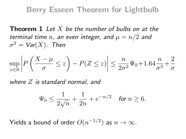
Berry Esseen Theorem for Lightbulb
Theorem 1 Let X be the number of bulbs on at theterminal time n, an even integer, and µ = n/2 andσ2 = Var(X). Then
supz∈R
∣∣∣∣P (X − µσ≤ z)− P (Z ≤ z)
∣∣∣∣ ≤ n
2σ2Ψ0+1.64
n
σ3+
2
σ
where Z is standard normal and
Ψ0 ≤1
2√n
+1
2n+ e−n/2 for n ≥ 6.
Yields a bound of order O(n−1/2) as n→∞.
8

Composition Markov chains of multinomialtype
Considered by Zhou and Lange, such chains in general arebased on a d× d Markov transition matrix P whichdescribes the transition of a single particle in a system of nidentical particles, a subset of which is selected uniformly toundergo transition at each time step according to P .
Very complete spectral decompositions of such chains maybe available; this decomposition becomes essential to thecalculation of the Berry Esseen bound for this problem.
Ehrenfest chains, Hoare-Rahman chains, Kimura’s modelfor DNA base-pair substitution.
9
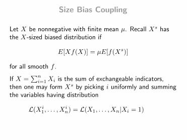
Size Bias Coupling
Let X be nonnegative with finite mean µ. Recall Xs hasthe X-sized biased distribution if
E[Xf(X)] = µE[f(Xs)]
for all smooth f .
If X =∑ni=1Xi is the sum of exchangeable indicators,
then one may form Xs by picking i uniformly and summingthe variables having distribution
L(Xi1, . . . , X
in) = L(X1, . . . , Xn|Xi = 1)
10

Size biased Coupling
With W = (X − µ)/σ, and W s = (Xs − µ)/σ,
E (h(W )− Eh(Z))
= E (f ′(W )−Wf(W ))
= E(f ′(W )− µ
σ(f(W s)− f(W ))
)= E
(f ′(W )(1− µ
σ(W s −W ))
−µσ
∫ W s−W
0
(f ′(W + t)− f ′(W ))dt
).
When monotone W s ≥W .
11

Concentration Inequality
Size bias version of exchangeable pair concentrationinequality of Shao and Su (2005).
Lemma 1 Let X be a nonnegative random variable withmean µ and variance σ2, both finite and positive, and letXs be given on the same space as X, having the X sizebiased distribution and satisfying Xs ≥ X. Then withW = (X − µ)/σ and W s = (Xs − µ)/σ,for any z ∈ R and a ≥ 0,
µ
σE(W s −W )1{W s−W≤a}1{z≤W≤z+a} ≤ a.
12
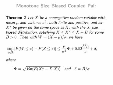
Monotone Size Biased Coupled Pair
Theorem 2 Let X be a nonnegative random variable withmean µ and variance σ2, both finite and positive, and letXs be given on the same space as X, with the X sizebiased distribution, satisfying X ≤ Xs ≤ X +B for someB > 0. Then with W = (X − µ)/σ, we have
supz∈R|P (W ≤ z)− P (Z ≤ z)| ≤ µ
σ2Ψ + 0.82
δ2µ
σ+ δ,
where
Ψ =√
Var(E(Xs −X|X)) and δ = B/σ.
13

Size biased coupling: Lightbulb
The number of bulbs on at time n is
X =
n∑k=1
Xk,
where Xk is the indicator that bulb k is on. Need to selectbulb at random, and turn it on if not already, keepingcorrect conditional distribution, and without greatlyaffecting the status of the other bulbs.
14

Size biased coupling: Lightbulb
The number of bulbs on at time n is
X =
n∑k=1
Xk,
where Xk is the indicator that bulb k is on. Need to selectbulb at random, and turn it on if not already, keepingcorrect conditional distribution, and without greatlyaffecting the status of the other bulbs.
With Xrk the switch variable of bulb k at time r, we have
Xk =
(n∑r=0
Xrk
)mod 2.
15

Size biased coupling: Lightbulb
Let n = 2m and X = {Xrk, r, k = 1, . . . , n}. For givenbulb i, if Xi = 1 then set Xi = X.
Otherwise J i ∼ U{j : Xn/2,j = 1−Xn/2,i}, independentof {Xrk : r 6= n/2, k = 1, . . . , n}. Let Xi have components
Xirk =
Xrk r 6= n/2Xn/2,k r = n/2, k 6∈ {i, J i}Xn/2,Ji r = n/2, k = iXn/2,i r = n/2, k = J i.
16

Size biased coupling: Lightbulb
In words, if Xi = 0 then uniformly select a j whose switchvariable Xn/2,j at stage n/2 is opposite to Xn/2,i, andinterchange.
17

Size biased coupling: Lightbulb
In words, if Xi = 0 then uniformly select a j whose switchvariable Xn/2,j at stage n/2 is opposite to Xn/2,i, andinterchange.
If I is the uniformly chosen index, and J the index of thebulb with opposite status at stage n/2, then
Xs −X = 21{XI=0,XJ=0}.
The coupling is monotone and bounded.
18

Conditional Variance Calculation, n = 2m
With F the σ-algebra generated by the switch variables X,
E
(Xs −X
∣∣∣∣ F) =4
n2
∑i 6=j
1{Xi=0,Xj=0,Xn/2,i=0,Xn/2,j=1}.
19

Conditional Variance Calculation, n = 2m
With F the σ-algebra generated by the switch variables X,
E
(Xs −X
∣∣∣∣ F) =4
n2
∑i 6=j
1{Xi=0,Xj=0,Xn/2,i=0,Xn/2,j=1}.
The variance calculation requires the computation of (four)joint probabilities such as g2,2,n,(1,...,n),n/2,(gα,β,n,s,l)
P (Xi1 = 0, Xj1 = 0, Xi2 = 0, Xj2 = 0,
Xn/2,i1 = 0, Xn/2,j1 = 1, Xn/2,i2 = 0, Xn/2,j2 = 1).
Conditioning on switches at stage n/2 they later become‘initial conditions.’
20

Spectral Decomposition
For a given subset of b of the n bulbs, the eigenvalues ofone, and multiple steps of the chain are given by
λn,b,s =
b∑t=0
(b
t
)(−2)t
(s)t(n)t
and λn,b,s =
k∏r=1
λn,b,sr ,
where (n)k = n(n− 1) · · · (n− k + 1) denotes the fallingfactorial, and the empty product is 1.
21

Spectrum of Composition Markov Chains ofMultinomial Type
In the case of the lightbulb chain there are d = 2 states andthe transition matrix P of a single bulb is given by
P =
[0 11 0
].
With b ∈ {0, 1, . . . , n} let Pn,b,s be the 2b × 2b transitionmatrix of a subset of size b of the n total lightbulbs when sof the n bulbs are selected uniformly to be switched.Letting Pn,0,s = 1 for all n and s, and I2 the 2× 2 identitymatrix, for n ≥ 1 the matrix Pn,b,s is given recursively by
Pn,b,s =s
n(P ⊗ Pn−1,b−1,s−1) + (1− s
n) (I2 ⊗ Pn−1,b−1,s) .
22

Spectral Decomposition
Transition matrices are simultaneously diagonalizable by
Pn,b,s = ⊗bT−1Γn,b,s ⊗b T,
where Γn,b,s = diag(λn,a1,s, . . . , λn,a2b ,s), e.g.,
a1 = (0, 1), a2 = (0, 1, 1, 2) and a3 = (0, 1, 1, 2, 1, 2, 2, 3),
and
T =1√2
[1 1−1 1
].
23

Spectral Decomposition
For calculation of g2,2,n,(1,...,n),n/2,
P (Xi1 = 0, Xj1 = 0, Xi2 = 0, Xj2 = 0,
Xn/2,i1 = 0, Xn/2,j1 = 1, Xn/2,i2 = 0, Xn/2,j2 = 1),
spectral decomposition yields
g2,2,n,s,l =1
16(1− 2λn,2,sl + λn,4,sl)
(sl)2(n− sl)2(n)4
,
where
sl = (s1, . . . , sl−1, sl+1, . . . , sn).
24
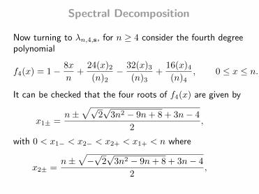
Spectral Decomposition
Now turning to λn,4,s, for n ≥ 4 consider the fourth degreepolynomial
f4(x) = 1− 8x
n+
24(x)2(n)2
− 32(x)3(n)3
+16(x)4(n)4
, 0 ≤ x ≤ n.
It can be checked that the four roots of f4(x) are given by
x1± =n±
√√2√
3n2 − 9n+ 8 + 3n− 4
2,
with 0 < x1− < x2− < x2+ < x1+ < n where
x2± =n±
√−√
2√
3n2 − 9n+ 8 + 3n− 4
2,
25
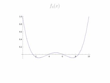
f4(x)
2 4 6 8 10
0.2
0.4
0.6
0.8
1.0
26

Need Bounds to compute ConditionalVariance
|f4(x)| ≤{ 6
(n−3)2 for x ∈ [x1−, x1+]
f22 (x) for x 6∈ [x1−, x1+], x ∈ [0, n].
where
f2(x) = 1− 4x
n+
4(x)2(n)2
, 0 ≤ x ≤ n.
27

λn,4,s
|λn,4,s| =bx1−c∏s=0
|λn,4,s|∏s∈u|λn,4,s|
n∏s=dx1+e
|λn,4,s|
Obtain
|λn,4,s| ≤1
2e−n for n ≥ 6,
for s = (1, 2, . . . , n/2− 1, n/2 + 1, . . . , n).
28
Berry Esseen Theorem for Lightbulb
Theorem 1 Let X be the number of bulbs on at theterminal time n, an even integer, and µ = n/2 andσ2 = Var(X). Then
supz∈R
∣∣∣∣P (X − µσ≤ z)− P (Z ≤ z)
∣∣∣∣ ≤ n
2σ2Ψ0+1.64
n
σ3+
2
σ
where Z is standard normal, and
Ψ0 ≤1
2√n
+1
2n+ e−n/2 for n ≥ 6.
Yields a bound of order O(n−1/2) as n→∞.
29

Stein’s Method for the Lightbulb Process
I hope that the talk was clear and illuminating
30

To Louis:
Thank you for all your hard work, and Happy Birthday!
31