A benchmark comparison of spontaneous subduction models – Towards a

free surface

H. Schmeling1, A.Y. Babeyko1,2, A. Enns1, C. Faccenna3, F. Funiciello3, T. Gerya4, G.J.

Golabek1,4, S. Grigull1,5 , B.J.P. Kaus4,7, G. Morra3,4, S. M. Schmalholz6, J. van Hunen8

1Goethe University, Institute of Earth Sciences, Frankfurt, Germany, Altenhöferallee 1, 60438 Frankfurt, schmeling@geophysik.uni-frankfurt.de

2Deutsches GeoForschungsZentrum, Telegrafenberg, 14473 Potsdam, Germany

3Dip. Scienze Geologiche, Università degli Studi « Roma TRE , Largo S.Leonardo Murialdo

1, 00146 Roma, Italy (ffunicie@uniroma3.it; faccenna@uniroma3.it)

4Geophysical Fluid Dynamics Group, Institute of Geophysics, Department of Geosciences, Swiss Federal Institute of Technology (ETH-Zurich), CH-8093 Zurich, Switzerland,

taras.gerya@erdw.ethz.ch, kaus@erdw.ethz.ch

5School of Geography, Environment and Earth Sciences (SGEES), Victoria University of Wellington, PO Box 600, Wellington, New Zealand

6 Geological Institut, ETH Zurich, Leonhardstrasse 19, 8092-Zurich Switzerland schmalholz@erdw.ethz.ch

7Department of Earth Sciences, University of Southern California, 3651 Trousdale Parkway, Los Angeles, CA-90089-740, USA.

8 Durham University, Department of Earth Sciences, Science Site, Durham, DH1 3LE, United

Kingdom, jeroen.van-hunen@durham.ac.uk

Preprint

Aug, 2008

Phys. Earth Planet. Int., in press.

2

Abstract

Numerically modelling the dynamics of a self-consistently subducting lithosphere is a

challenging task because of the decoupling problems of the slab from the free surface. We

address this problem with a benchmark comparison between various numerical codes

(Eulerian and Lagrangian, Finite Element and Finite Difference, with and without markers) as

well as a laboratory experiment. The benchmark test consists of three prescribed setups of

viscous flow, driven by compositional buoyancy, and with a low viscosity, zero-density top layer

to approximate a free surface. Alternatively, a fully free surface is assumed. Our results with a

weak top layer indicate that the convergence of the subduction behaviour with increasing

resolution strongly depends on the averaging scheme for viscosity near moving rheological

boundaries. Harmonic means result in fastest subduction, arithmetic means produces slow

subduction and geometric mean results in intermediate behaviour. A few cases with the

infinite norm scheme have been tested and result in convergence behaviour between that of

arithmetic and geometric averaging. Satisfactory convergence of results is only reached in one

case with a very strong slab, while for the other cases complete convergence appears mostly

beyond presently feasible grid resolution. Analysing the behaviour of the weak zero-density top

layer reveals that this problem is caused by the entrainment of the weak material into a

lubrication layer on top of the subducting slab whose thickness turns out to be smaller than

even the finest grid resolution. Agreement between the free surface runs and the weak top

layer models is satisfactory only if both approaches use high resolution. Comparison of

numerical models with a free surface laboratory experiment shows that (1) Lagrangian-based

free-surface numerical models can closely reproduce the laboratory experiments provided that

sufficient numerical resolution is employed and (2) Eulerian-based codes with a weak surface

layer reproduce the experiment if harmonic or geometric averaging of viscosity is used. The

harmonic mean is also preferred if circular high viscosity bodies with or without a lubrication

layer are considered. We conclude that modelling the free surface of subduction by a weak

zero-density layer gives good results for highest resolutions, but otherwise care has to be

taken in 1) handling the associated entrainment and formation of a lubrication layer and 2)

choosing the appropriate averaging scheme for viscosity at rheological boundaries.

3

1. Introduction

While dynamically modelling of subduction has been an issue in the geodynamical literature

since a long time (e.g. Jacoby 1976; Jacoby and Schmeling, 1982) only recently a vast

number of numerical and laboratory models have been developed in an attempt to understand

the dynamics of self-consistently forming subduction zones (Bellahsen et al., 2005,

Funiciello, et al., 2003a,b, Schmeling et al., 1999, Tetzlaff and Schmeling, 2001, Capitanio et

al., 2007, and others). The term "self-consistent" emphasizes that the formation of the trench

and the sinking of the slab is driven by internal forces only and without invoking prescribed

zones of weakness. One of the major problems in all models is to formulate and apply a

method to decouple the subducting slab from the surface or the overriding plate. While early

modellers simply assumed a sufficiently large region near the trench in which the mantle was

artificially weakened, other models invoked more complex rheologies or neglected the

overriding plate at all (Schmeling and Jacoby, 1981, Becker at al, 1999; Funiciello, et al.,

2004; 2006; Kincaid & Olson, 1987; Martinod et al, 2005; Schellart et al., 2004a, b, 2005;

Stegman et al., 2006).

Laboratory models have the possibility to simulate realistic geologic features using complex

rheologies and at the same time having the advantage of an intrinsically 3-D approach.

However, 3-D aspects are often suppressed using laterally homogeneous slabs affected by box

boundary effects (Kincaid and Olson, 1987; Shemenda, 1992) or by using 2-D feeding pipes

to inject the slab into a density/viscosity layered fluid (Griffiths and Turner, 1988; Griffiths et

al., 1995; Guillou-Frottier et al., 1995). 3-D laboratory models including lateral slab migration

have been recently realized prescribing kinematically the trench movement by Buttles and

Olson, (1998) and Kincaid and Griffith (2003) and dynamically self-consistently by Faccenna

et al., (2001) and Funiciello et al., (2003; 2004, 2005) and Schellart, (2004a, b, 2005). 3-D

numerical subduction models have been studied e.g. by a Stegman et al. (2006), Schellart et

al. (2007).

All these approaches can be divided into two classes: In one class subduction is

kinematically or rheologically prescribed by kinematic boundary conditions of weak

decoupling zones. In the other class the decoupling zones evolves self-consistently. Our

benchmark addresses this second class of models. Furthermore our setup studies a slab

without an overriding plate. Thus the dynamics reveals the behaviour of a subducting slab as

it decouples from the free surface without being influenced by another plate.

Although our benchmark definition might look quite simple, as it describes a purely

viscous, isothermal fluid dynamical problem with linear creeping rheology, and the viscosity

4

contrasts are 104 at most, it turns out to be a very challenging test. This is because of the

decoupling mechanism acting in real systems in which dense bodies detach from a surface,

even if they are purely viscous: Layers of different composition interact dynamically, are

smeared out and turn into lubrication layers. As the numerical resolution of our codes is

limited, such fluid dynamical scenarios easily exceed the limitations of even high resolution

runs. To explore how these limits are reached by different codes and what can be done to

tackle these resolution problems is one of the motivations of the present benchmark.

Our approach is three-fold. In one set of tests (case 1) we try to benchmark the process of

subduction approximating the subduction zone to be overlain by a soft buoyant layer (“sticky

air” or an artificial layer whose lowermost part consists of water rich, weak sediments, in

short "soft sediments") and compare it to subduction models with a free surface. As it will

turn out, the soft material will be entrained, lubricating the subducting slab, and the

subducting slab is decoupled from the overriding mantle in a self-consistent way. However,

the lubricating layer will be very thin, its thickness is beyond the resolution of our models.

Consequently, to achieve convergence of the different codes will be difficult.

Notwithstanding, such model approaches are frequently discussed in the literature. Therefore,

it is interesting to study how the different methods deal with this decoupling / lubricating

problem, how the algorithms of determining the effective viscosity at the lubrication region

handle the problem, and how they compare to models with a free surface.

In a second approach (case 2), an attempt is made to achieve convergent results of the

different codes. We will define a modified setup, namely one without the formation of a thin

lubricating layer. In this setup, the viscosity of the overlying layer will be chosen as equal to

the mantle viscosity. Consequently, no lubrication layer can form, and one should expect that

the resulting evolution of subduction should converge among the different codes. It should be

emphasized, that we do not suggest this setup to be realistic in the sense of subduction

dynamics, but it is a reasonable fluid dynamic setup to test codes which model the evolution

of a triple point associated with a subduction zone. For constant viscosity thermal convection

the role of such a triple point on entrainment of material with a different density has already

been benchmarked by van Keken et al. (1997).

Thirdly (case 3), we benchmark a laboratory subduction model with a free surface and try to

reproduce it as close as possible by numerical models with a weak top layer or with free

surface numerical models.

5

In the section 5, we present a well resolved case of a Stokes flow problem with and without

a lubrication layer to test the applicability of our algorithms of determining the effective

viscosity near compositional rheological boundaries.

2. Definition of cases

2.1 Governing equations

The benchmark is defined as a purely viscous fluid dynamic problem. We assume an

incompressible fluid, in which driving density fields are advected with the flow. Then the

problem can be described by the equations of conservation of mass

)1(0v =⋅∇rr

and the equation of momentum

)2(0egxv

xv

xP 3k

i

j

j

ik

j=−

⎥⎥⎦

⎤

⎢⎢⎣

⎡

⎟⎟⎠

⎞⎜⎜⎝

⎛

∂

∂+

∂∂

∂∂

+∇−rr

ρη

where is the velocity, P the pressure, x the coordinates, ηvr k the viscosity of composition k,

ρk the density of composition k, g gravity acceleration, and 3er the unit vector in vertical

upward direction. The viscosity and the density are advected with the flow. The

corresponding advection equation is given by

)3(0Cvt

Ck

k =∇⋅+∂∂ rr

where Ck is the concentration of the k-th composition. Ck is equal 1 in a region occupied by

composition k and 0 elsewhere.

2.2 Model setup

The 2D model setup for case 1 and 2 is shown in Fig. 1. It is defined by a layer of 750 km

thickness and 3000 km width. The initial condition is specified by a mantle of 700 km

thickness, overlain by a 50 km thick soft surface layer mimicking "sticky air" or "soft

sediments". The mantle layer consists of a highly viscous, dense lithosphere (ρl = 3300 kg/m3,

6

ηl = 1023 Pa s, initial thickness of 100 km) and an ambient mantle with ρm = 3200 kg/m3, ηm =

1021 Pa s. The surface layer of initially 50 km thickness has a density ρs = 0 kg/m3 and a

viscosity of either ηs = 1019 Pa s or ηs = 1021 Pa s and a free slip top. In order to trigger

subduction and mechanical decoupling of the slab from the surface in a most direct and

simple way the slab tip is already penetrating into the mantle as deep as 200 km (from the top

of the mantle). This configuration with a 90° corner avoids that time-dependent bending

might mask the detachment of the slab from the surface. The mechanical boundary conditions

are reflective (free slip), implying the slab being attached to the right boundary.

The model setup for the free surface case is identical to the setup described above, only the

weak surface layer is removed, and the surface boundary condition is free.

The model setup for the laboratory experiments and the corresponding numerical

experiments (case 3) is somewhat different and will be described in detail in section 3.3.

3. Methods

3.1. The participating codes

FDCON

The code FDCON (used by authors Schmeling, Golabek, Enns, and Grigull) is a finite

difference code. Equations 1 and 2 are rewritten as the biharmonic equation in terms of the

stream function and variable viscosity (e.g. Schmeling and Marquart, 1991). The FD

formulation of the biharmonic equation results in a symmetric system of linear equations,

which is directly solved by Cholesky decomposition. The advection equation is solved by a

marker approach (e.g. Weinberg and Schmeling, 1992). The region is filled completely with

markers which carry the information of composition k. The concentration Ck of composition k

at any FD grid point is determined by the number of markers of composition k found within a

FD-cell sized area around the grid point divided by the total number of markers present in the

same cell. The density and viscosity at any grid point are determined by Ck - weighted

averaging using either the harmonic, the geometric or the arithmetic mean (see below). The

markers are advanced by a 4-th order Runge-Kutta-scheme, combined with a predictor-

corrector step. For this predictor-corrector step, markers are provisionally advanced by two

first order Eulerian steps. The Navier Stokes equation is solved for these preliminary steps to

obtain the corresponding velocity fields. These velocity fields are then taken for the full 4th

order Runge-Kutta step to advance the markers.

7

I2VIS, I2ELVIS

Both the viscous code I2VIS (used by author Gerya) and the viscoelastic code I2ELVIS are

based on a combination of finite-differences (pressure-velocity formulation on fully staggered

grid) with marker-in-cell technique (Gerya and Yuen, 2003a: Gerya and Yuen, 2007).

Markers carry information on composition (which is used to define density, viscosity and

shear modulus) and stresses (in viscoelastic case). Viscosity, density and stresses (in

viscoelastic case) are interpolated from markers to nodes by using bilinear distance-dependent

schemes. In I2ELVIS the shear modulus for viscous runs was taken 6.7⋅1030 Pa and the bulk

modulus was taken infinity (incompressible fluid). Obviously with a time step of 104 years

and a viscosity of the slab of 1023 Pa s there is no elastic deformation component. The

markers are advanced by a 4-th order in space 1st order in time Runge-Kutta-scheme. The

runs done with I2ELVIS differ from those with I2VIS in that they average the viscosity

around nodes more locally. In I2ELVIS averaging from markers to a node is done from

markers found in 1 grid cell around the node (i.e. within 0.5 grid step). Averaging in I2ELVIS

is done separately for different nodal points corresponding to shear (interceptions of grid

lines) and normal (centres of cells) stress components. In I2VIS averaging from markers to

nodes is first uniformly done for nodal points corresponding to shear stress components (i.e.

for intersections of grid lines) from markers found in 2x2=4 grid cells around each nodes (i.e.

within 1.0 grid step). Then viscosity for normal stress components is computed for centres of

cells by averaging viscosity from 4 surrounding “shear viscosity nodes” (i.e. averaging is

effectively from 3x3=9 cells, within 1.5 grid step). Both codes use the optional possibility of

refinement locally in a 100-800 km wide and 10-20 km deep area (Swiss-cross-grid following

the trench). Therefore, the subsequent models converge better for the initial 10-20 Myr of the

model development.

LAPEX-2D

This code (used by author Babeyko) solves for balances of mass, momentum and energy

through an explicit Lagrangian finite difference technique (FLAC-type) (Cundall & Board

1988; Poliakov et al. 1993; Babeyko et al. 2002) combined with particle-in-cell method

(Sulsky et al., 1995). The solution proceeds on a moving Lagrangian grid by explicit time

integration of conservation equations. For that reason, the inertial term tviinert ∂∂ρ is

included into the right-hand side of the momentum conservation equation (Eq.2). Here inertial

density actually plays a role of parameter of dynamic relaxation. Incorporation of the

inertial term allows explicit time integration of nodal velocities and displacement

inertρ

8

increaments, thus “driving” the solution towards quasi-static equilibrium. The magnitude of

the inertial term is kept small in comparison to tectonic forces, typically, 10-3 – 10-5, so the

solution remains quasi-static. In comparison to the classical implicit finite element algorithm,

memory requirements of this method are very moderate, since no global matrices are formed

and inverted. Accordingly, computational costs for one time step are very low. However,

explicit time integration imposes very strict restrictions on the magnitude of the calculational

time step – for typical geodynamic application the stable Courant time step has an order of 1-

10 years. Being a disadvantage of this method, the small computational time step allows,

however, treatment of any physical non-linearity (such as plastic flow, for example) in a

natural way, without any additional iterations and problems with convergence. A principal

restriction in LAPEX-2D, which partly limited it's suitability for the present benchmark setup,

is the requirement of non-zero material density. Thus benchmarks with zero-density 'sticky

air' soft layer were not performed with LAPEX-2D. The algorithm is easy parallelizable.

LAPEX-2D has a principally visco-elastic solver. The explicit numerical scheme of stress

update at each computational time step directly exploits the elastic constitutional law. Thus,

elasticity cannot be completely 'switched-off'. In the present models, the slab was assigned the

elastic properties of olivine, i.e., Young's modulus E=184 GPa and Poisson's ratio of 0.244.

Together with slab viscosity of 1023 Pa s these elastic properties correspond to the Maxwell

relaxation time of 40 kyr, which is much less than the characteristic model time. Thus, the

behaviour of the slab in LAPEX-2D is effectively viscous.

Solution on the moving Lagrangian grid becomes non-accurate when the grid becomes too

distorted. At this point remeshing should take place. During remeshing the new grid is built,

and solution variables are interpolated from the old distorted grid. This procedure of

remeshing is inevitably related to the problem of numerical diffusion. In the case of history-

dependent solution, like presence of elastic stresses, and strong stress gradients (e.g.,

subducting slab versus its surrounding), uncontrollable numerical diffusion might strongly

affect the solution. In order to sustain it, we have implemented in our code a particle-in-cell,

or material point technique (Sulsky et al., 1995). In this approach, particles, which are

distributed throughout the mesh, are more than simple material tracers. In LAPEX-2D,

particles, typically 30 - 60 per element, track not only material properties but also all history-

depending variables including full strain and stress tensors. Between remeshings, particles

provide no additional computational costs since they are frozen into the moving Lagrangian

grid composed of constant-stress triangles, and there is no need to update particle properties at

this stage. Additional computational efforts arise only during remeshing. First, stress and

9

strain increments accumulated since the previous remeshing are mapped from Lagrangian

elements to particles. After the new mesh is constructed, stresses and strains are back-

projected from particles onto the new grid.

CITCOM

The code Citcom (used by author van Hunen) is a finite element code (Moresi and Solomatov,

1995; Moresi and Gurnis, 1996; Zhong et al., 2000). The finite elements are bi-linear

rectangles, with a linear velocity and a constant pressure. Interpolation of composition is done

per element and directly applied to the integration points. The code uses an iterative multigrid

solution method for the Stokes Equation. Equations (1) and (2) in their discrete form are

written as:

)4(fBpAu =+

)5(0=uBT

This system of equations is solved with some form of the Uzawa iteration scheme: Equation

4 is solved iteratively with a Gauss-Seidel multigrid method, while applying Equation 5 as a

constraint. The augmented Lagrangian formulation is used to improve convergence of the

pressure field for large viscosity variations. A marker approach is used to solve the advection

equation (3): the computational domain is filled completely with markers (approximately 40

markers per finite element), which carry the composition. Markers are advected using a

second order Runge-Kutta scheme. Interpolation from the markers onto the integration points

of the finite element mesh is done by a geometric weighted average of the marker values over

each element (i.e. one value per element).

ABAQUS with remeshing

An adaptive solid mechanical Finite Element Method (Abaqus Standard) (used by author

Morra) that uses the tangent operator matrix is employed for calculating the deformation of

the mantle. In order to avoid excessive deformation, every 1Ma a remeshing algorithm re-

interpolates the variables to the initial mesh. The materials are traced using a field defined at

the nodes (field1: 0=air, 1 = mantle ; field2: 0 = mantle, 1=lithosphere) and the material

properties are calculated interpolating the field at the 4 nodes around each linear quadratic

element. Rheology is implemented in all configurations, using geometric, arithmetic and

10

harmonic mean. For the viscous runs the elastic modulus is increased by of 2 orders of

magnitude compared to the real value in nature (i.e. 1013 Pa vs.. 1011 Pa), which reduces the

Maxwell time by 2 orders of magnitude, therefore inhibiting elasticity (stresses are dissipated

immediately, with virtually no delay). .

LaMEM

LaMEM (used by author Kaus) is a thermo-mechanical finite element code that solves the

governing equations for Stokes flow in parallel in a 3D domain using Uzawa iterations for

incompressibility and direct, iterative or multigrid solvers (based on the PETSc package). A

velocity-pressure formulation is employed with either Q1P0 (linear) elements or Q2P-1

elements (quadratic for velocity and linear discontinuous for pressure). To facilitate

comparison with similar FEM methods in this benchmark study (such as CitCOM), all

computations have been performed with linear elements. Tracers are used to advect material

properties as well as stress tensors. Material properties are computed at integration points by

arithmetic averaging from the nearest tracers. In free surface runs, the properties at the

integration points are employed for calculations. In selected cases, the values from all

integration points in an element are homogenized through arithmetic, geometric or harmonic

averaging (which thus yields one value of viscosity per cell). Tracer advection is done

through mapping of global tracer coordinates to local ones, after which the element is

deformed, and tracer locations are mapped back to global coordinates. LaMEM can be

employed in an Eulerian mode, in a purely Lagrangian mode, or in an Arbitrary Lagrangian-

Eulerian (ALE) mode, in which some elements are deformed (typically close to the free

surface) but others are fix. The ALE mode employs remeshing after each time step.

An advantage of LaMEM is that it can handle self-consistent free surface deformation, while

simultaneously solving the Stokes equation in an implicit manner. In free-surface simulations

the ALE approach is used with remeshing based on the free-surface deformations. Remeshing

is done at each timestep, and a new free surface is created from the old one by linear

interpolation on regular x- coordinates. If angles larger than 25 degrees occur at the free

surface after remeshing, a kinematic redistribution algorithm is employed that distributes the

fluid over adjacent nodes in a mass conservative manner (until angles<25 degrees).

FEMS-2D

FEMS-2D (used by author Schmalholz) is a finite element code for simulating slow

incompressible flows in two dimensions (Frehner and Schmalholz, 2006; Schmalholz, 2006)

11

and is written in MATLAB (The MathWorks). The algorithm is based on a mixed velocity-

pressure formulation (e.g., Hughes, 1987). Two different elements can be used: (i) the

isoparametric Q2-P1 9-node quadrilateral element using 9 integration points, a biquadratic

velocity approximation and a linear discontinuous pressure approximation or (ii) the

isoparameteric P2-P1 7-node triangular element using 7 integration points, a quadratic velocity

approximation and a linear discontinuous pressure approximation (e.g., Cuvelier et al. 1986;

Hughes, 1987; Bathe, 1996). The higher order elements for the velocities are used in

combination with linear elements for the pressure. This so-called mixed velocity-pressure

formulation is especially accurate for pressure calculations for incompressible flows (which

are not calculated using a stream function Ansatz). The higher order elements should here not

matter concerning the overall accuracy of the calculated flow field. Both elements satisfy the

inf-sup condition guaranteeing numerical stability for incompressible flows. Uzawa-type

iterations are used to achieve incompressible flow. For both elements the pressure is

eliminated on the element level. For the presented numerical subduction simulations the

triangular elements are used. The applied mesh generator is Triangle developed by J.

Shewchuk (Shewchuk, 1996, www.cs.cmu.edu/~quake/triangle.html). An algorithm written

in MATLAB (developed and provided by Dani Schmid, PGP, University of Oslo, Norway) is

used to link the mesh generator Triangle with FEMS-2D. After each time step the coordinates

of the nodes are updated by adding the corresponding displacements which result from the

product of the calculated velocities times the time step (explicit time integration). The new

velocity field is then calculated for the new nodal coordinates.

Recently, the matrix assembly algorithm and solver developed by Dabrowski et al. (2008)

was implemented in FEMS-2D which shortened the computation time significantly. This

version has been named MILAMIN (used by authors Schmalholz and Kaus). Tests have

shown that the results are identical to models with FEMS-2D.

Due to the applied Lagrangian approach the numerical mesh is deformed with the

calculated velocities. When the finite element triangles are too strongly deformed, the finite

element mesh is re-meshed but the contour lines defining the geometry of the mantle and the

slab remain unchanged. There is also one point at the free surface at which the mantle surface

and the slab surface are identical, i.e. the point defining the trench. During the slab subduction

the mantle is overriding the slab and the contour line defining the free surface of the mantle

gets overturned, which is unrealistic. Therefore, once the mantle surface exceeds a critical

angle (between 10 and 90 degrees), the trench point is moved upwards along the contour line

defining the slab surface. Two different approaches have been applied: in the first approach

12

the trench point is simply moved upwards to the next nodal point on the contour line of the

slab surface and the mantle surface is additionally smoothed. This approach does not

guarantee a strict mass conservation. In the second approach, a new trench point is generated

at the slab surface so that the surface of the mantle exhibits a predefined angle at the trench

(here 10 degrees) and additionally the mass of mantle material is conserved. It was found that

when the numerical resolution is sufficiently large (i.e. the results of each algorithm do not

change significantly anymore with higher resolution) around the trench, both approaches yield

nearly identical results. The stepwise change of the trench location caused by the adjustment

of the contour lines can be physically interpreted with some kind of stick-slip behaviour,

where stresses first build up and are then released by the slip of mantle material along the

surface of the slab.

3.2. Viscosity averaging

At compositional boundaries all codes have the problem of either to map the viscosity (and

density) advected by the markers to the FD- or FE grid, or to interpolate viscosities from a

deformed mesh to a remeshed configuration. This is done by using either of the following

averaging laws:

Harmonic mean:

)6(1

2

2

1

1

ηηηCC

ave

+=

Arithmetic mean:

)7(2211 ηηη CCave +=

Geometric mean:

)8(2121CC

ave ηηη =

Here ηi is the viscosity of composition i, and Ci is the relative volumetric fraction of

composition i in the vicinity of the FE- or FD-node at which the effective viscosity ηave is

needed. A physical discussion of the above laws will be presented below.

Another viscosity averaging scheme which deliberately avoids any a priori assumptions

about the averaging process, or any information about marker distributions on a scale below

the grid resolution is the "infinite norm average":

)9(,...,1,:, matikkave niCCkwith =≥=ηη

13

where nmat is the total number of compositions. Equation (9) simply states that the material

which has most particles in a cell determines the material properties of that cell.

In the subsequent sections we essentially use and compare models with the harmonic,

arithmetic and geometric means, and apply the infinite norm average only in one resolution

test. In section 5 (Discussion) the infinite norm scheme is discussed and quantified for a 2D-

Stokes flow problem..

3.3 Laboratory experiments and set up of corresponding numerical runs

We (authors Funiciello and Faccenna) use silicone putty (Rhodrosil Gomme, PBDMS + iron

fillers) and glucose syrup as analogue of the lithosphere and upper mantle, respectively.

Silicone putty is a visco-elastic material behaving viscously at experimental strain rates

(Weijermars and Schmeling, 1986) since the deformation time-scale is always larger than its

Maxwell relaxation time (about 1 s). Glucose syrup is a transparent Newtonian low-viscosity

fluid. These materials have been selected to achieve the standard scaling procedure for

stresses scaled down for length, density and viscosity in a natural gravity field (gmodel = gnature)

as described by Weijermars and Schmeling (1986) and Davy and Cobbold (1991).

The layered system, where densities and viscosities are assumed as constant over the

thickness of the individual layers, is arranged in a transparent Plexiglas tank (Fig. 2a). The

subducting plate is fixed to the box in the far field ("fixed ridge" see Kincaid and Olson,

1987). 3-D natural aspects of laboratory models are minimized using slabs as large as the

width of the box (w = b). It allows to consider in first approximation the system as two-

dimensional for comparison with the numerical models of the present benchmark. The box

sides are lubricated with Vaseline to avoid sticking effects of the slab with the box

boundaries.

The subduction process is manually started by forcing downward the leading edge of the

silicone plate into the glucose to a depth of 3.1 cm (corresponding to about 200 km in nature)

at an angle of ~30o. In Figure 2a and Table 1 we summarized the characteristics of the

selected experiment we describe in the present paper. For more detailed explanations see

Funiciello et al., 2003, 2004. The experiment is monitored over its entire duration by two

digital cameras both in the lateral and top views. Kinematic and geometric parameters (trench

retreat, dip of the slab) are afterwards quantified by means of image analysis tools (software

DIAna Image Analysis). The measurement error was ±0.1 cm.

The laboratory set up is taken to define a corresponding 2D numerical set up (Fig. 2b). As

these experiments are carried out by both the codes with a free surface and with a soft surface

14

layer ("sticky air"), both alternative setups are depicted in Fig 2b. Based on the photograph of

the laboratory model at time equal zero, the initial dip angle and length of the leading edge of

the slab are chosen as 34° and 6 cm, respectively,

4. Results

We first present results of case 1 with a weak decoupling layer (1019 Pa s), which leads to the

entrainment of weak material and effective lubrication of the upper side of the subducting

slab. We then show the results of the free surface runs. This will be followed by the non-

lubrication models (case 2) with a “weak layer” of 1021 Pa s. Finally (case 3) the laboratory

result and the corresponding numerical runs will be shown.

4.1 Models with weak decoupling layer (case 1)

These models have been run with different resolutions by the codes and are summarized in

Table 2. The typical behaviour of a case 1 model is shown in Fig 3. At time 0 instantaneously

high vertical flow velocities of the order of 5.4 cm/a are observed as the originally flat

mantle/lithosphere surface relaxes towards an isostatic equilibrium. This equilibrium is

approached after about 100 to 200 kyr, and is associated with a vertical offset at the trench of

about 4 km. This isostatic relaxation is confirmed by the codes FDCON (3.8 km after

180kyr), CITCOM (3.9km after 183 kyr),, I2ELVIS (4.7 km after 400 kyr) with an accuracy

of approximately 100 m, as well as by the free surface model LaMEM and FEMS-2D (both 4

km after 200 kyr) and LAPEX-2D (5.2 km after 2 Ma). During the following 20 Mio years

vertical velocities are small (order of 0.25 cm/yr). It takes a few tens of Mio years until the

slab successfully detaches from the surface. Rapidly it subducts through the upper mantle and

reaches the bottom of the box after some tens of Mio years. As the slab is fixed at the right

side of the model box, subduction is accompanied by considerable roll back with a horizontal

velocity of the order of 1 cm/yr.

4.1.1 Comparison of slab shapes

First we compare the shapes of the subducting slabs. As the temporal behaviour is different

(see below) we chose snapshots for stages at which the subducting slab has reached a depth of

approximately 400 km. As can be seen in Fig 4, the similar stages are reached at different

times. The geometries are quite similar on first order, but a detailed examination reveals some

15

differences: the FDCON case shows a slightly stronger thickening of the horizontal part of the

plate, associated with a larger trench retreat compared to the I2ELVIS-model. In the FDCON-

model the originally right angles at the edges of the slab front are less deformed than in the

I2ELVIS case. The CITCOM model has already subducted to a slightly greater depth than the

other two models, however, the trench retreat the same as for FDCON. A careful examination

of the three models shows that a thin layer of soft surface material is entrained on top of the

subducting slab. As will be discussed more in detail below, this layer is thinner than the grid

resolution of all of the models, thus its lubricating effect may differ from code to code. Most

importantly the lubrication effect depends on the way of determining the effective viscosity in

the entrainment region (see section 3.2). All three models shown in Fig 4 used geometric

means (equ. 8) for viscosity averaging, that is the reason for the first order similarity of the

geometries.

Fig. 5 show the effect of viscosity averaging on the shapes of the slabs. Note that the

snapshots are taken at different times, so that the slab tips have reached comparable levels.

The deformation of the slab tip is strongest for the case with the harmonic mean, which yields

the weakest effective viscosity, while the original shape of the rectangular slab is best

preserved for the stiffer arithmetic mean case. In arithmetic case, the bending is more

localized near the trench, as deeper parts of the slab have already undergone unbending during

the more slowly subduction. In the harmonic case, which are taken at shorter times,

unbending has not proceeded that far. The geometric mean case shows characteristics just in

between the other two cases.

4.1.2 Comparison of temporal behaviour

To compare the temporal behaviour of the different models Fig 6 shows the depth of the slab

as a function of time for different codes and highest resolutions each. Diagrams of the full set

of models with different resolutions is given in the Appendix A. In contrast to the others,

I2VIS and I2ELVIS also used of local refinement (curves with symbols). All models

(FDCON, I2VIS, I2ELVIS, CITCOM, LAPEX2D) using geometric mean (greenish curves)

lie close together and reach the 400 km depth level after 35 – 41 Myr. Interestingly

LAPEX2D used a higher weak layer viscosity of 1020 Pa s instead of 1019 and still shows

good agreement with the others who used the geometric mean.

The highest resolution uniform grid models using arithmetic mean for viscosity averaging

(FDCON and I2ELVIS) (bluish curves) show a significant slower subduction. Increasing the

grid resolution locally (on the expense of grid resolution far away from the trench area),

16

I2VIS with arithmetic means (blue curve with diamonds) shows a significant faster

subduction compared to the uniform grid, arithmetic mean models (blue curves) and lies close

to the slowest models with geometric means (greenish curves). Averaging the viscosity near

boundaries even more locally as is done by I2ELVIS (blue curve with squares) speeds up

subduction even more, entering the field of curves with the geometric mean.

However, testing the harmonic mean as a third reasonable possibility shows again a

dramatic effect: FDCON, I2VIS and I2ELVIS highest resolution models show (redish curves)

that subduction is now much faster than in the previous cases, even when using the highest

resolutions. However, locally refined models now show the tendency towards slower

subduction, these curves lie on the slower side of the set of the harmonic averaging models.

A resolution test of the models of case 1 with a weak top layer is shown in Fig 7 which

shows the time at which the slab tip passes the 400 km level as a function of the characteristic

grid size used in the runs. Increasing the resolution clearly shows that the curves with the

geometric or arithmetic means converge from high values towards a time between 34 and 38

Myr. The I2VIS and I2ELVIS runs with the harmonic mean show a trend of coming from

small values converging towards an asymptotic value between 25 and 30 Myr. FDCON

(harmonic) has the same asymptotic trend, but shows characteristic oscillations which are

strongly damped as the resolution increases. The frequency of these oscillations, which are

also observed for the geometric averaging models of FDCON, correlates with the frequency

with which a FD-grid line coincides with the compositional interface between the lithosphere

and the soft layer (non-connected crosses in Fig 7). The convergence behaviour of FDCON

with infinite norm scheme is similar to arithmetic averaging models, but the asymptotic trend

is not well defined.

In Fig 8. we show the temporal behaviour of the trench rollback evolution of our highest

resolution models for different rheological averaging schemes used. Only the results of

I2ELVIS and I2VIS are shown, as those allow for local grid refinement in the trench region.

During the first 15 - 20 Myr all models with local refined grids agree well with each other and

follow roughly the evolution of the uniform grid run with geometric mean. The uniform grid

models with harmonic or arithmetic mean significantly differ already from the beginning. At

later stages, t > 20 Myr, the retreat curves diverge, with the harmonic mean models retreating

fastest (redish curves) and the arithmetic mean curves retreating slowest (bluish curves). The

full set of models with different resolutions is shown in Appendix A, Fig. A2a to A2c.

From this comparison it becomes clear that the codes have some problems in correctly

solving the stated fluid dynamical problem (which should have a unique solution). They only

17

converge to roughly comparable subduction histories if the resolution is drastically increased.

Harmonic and arithmetic mean runs approach the geometric solution from opposite sides, runs

with geometric mean often seem to start from values closer to the asymptotic value. Yet,

extrapolation of these runs towards the exact solution is not fully satisfactory as the

differences between results obtained by different viscosity averaging methods are still large,

and asymptotic values of harmonic and other means do not yet coincide for the resolutions

used. In the next section we give an explanation for the diverse behaviour of our models in

terms of decoupling and lubrication.

4.1.3 Decoupling from the top - the role of entrainment of weak material

In order to examine the reason for the differences among the models with different viscosity

averaging, Fig. 9 presents a closer look at the details of one of our models. The marker

distributions show that a thin layer of the weak surface material is entrained on top of the

downgoing slab. This layer is only one to three markers wide (in this example, every 4th

marker is shown in every direction), thus lies below the resolution of the FD grid. As the

weak surface layer markers carry weak rheology, they decrease the effective viscosity within

a layer immediate above the downgoing slab, but only irregularly within distinct FD grid cells

as is visible by the irregular distribution of bluish FD cells (Fig 9 left). This lubrication helps

the subduction of the slab, however, it cannot be resolved adequately as the lubrication layer

is thinner than the grid resolution. We believe that such differences in non-resolvable

lubrication behaviour is the reason for the significant differences between the models if

different rheological averaging methods are used, and if the resolution is varied.

4.2 Free surface models

Case 1 has also been modeled by LAPEX2D, LaMEM and FEMS-2D assuming a free surface

instead of the weak surface layer (Fig. 10). These runs point out that the results depend

strongly on the numerical resolution that is employed. Low resolution is accompanied by a

higher resistance of the mantle at the trench region to flow and spread on top of the sinking

slab. Coarse elements do not well approximate the high curvatures at the tip of the

"overrolling" mantle wedge building up near the trench and make the surface geometrically

stiffer (or less flexible). This requires more strain until one of the surface elements at the tip

of the wedge gets overturned and re-meshing (i..e. 'slip' of one element) is performed. Large

elements cannot resolve this overturning and lead to ‘numerical locking’ – severe

underestimation of the correct solution by the accepted numerical approximation. This

18

numerical ‘locking effect’ is especially pronounced in the beginning of the slab sinking

process, when the mantle wedge loading is still small. Moreover, the results in Fig. 10 show

that low-resolution LaMEM and LAPEX2D runs probably demonstrate pertinent locking at

the mantle wedge even at later stages of subduction. Larger velocities and full decoupling of

the slab from the surface are only obtained for higher resolutions and re-meshing near the

trench.

In the FEMS-2D runs an unstructured mesh with a high resolution around the slab and low

resolution away from the slab has been used. Increasing the resolution in these runs mainly

increased the resolution away from the slab and made the mesh more regular. As the number

of markers in the marker chain specifying the slab shape was the same in the different runs,

the resolution directly around the slab was nearly identical in the runs. This is the reason for

almost identical curves for different resolutions. Thus, increasing the resolution in areas away

from the slab does not change the results. On the other hand, the time step has some effect on

the behaviour because remeshing is done once the light material becomes "overturned" while

overriding the slab. Bigger time steps lead to an earlier remeshing because the light material

becomes faster overturned.

Even for the highest resolutions there are still significant differences between the different

codes. We believe that these differences are due to the different remeshing schemes used,

particularly near the trench (see section 3.1). However, once the decoupling reached a quasi-

steady state, the subduction velocities of the FEMS-2D and LaMEM models are similar.

4.3 Models without a lubrication layer (case 2)

As has been shown in section 4.1, the entrainment of weak material helped decoupling of the

slab from the surface but did not lead to fully converging results when using different

viscosity averaging methods. Therefore we carried out a second comparison of results (case 2

models) for a model in which the “soft layer” had the viscosity ηs = 1021 Pa s, i.e. the same

viscosity as the mantle. The idea was, that if any entrainment of this layer takes place there

will be no lubrication between the slab and the ambient mantle. This model setup has been run

with different resolutions by the codes summarized in Table 3.

4.3.1 Comparison of slab shapes and temporal behaviour

The general behaviour of this case is shown in Fig. 11. During the first 40 Myr the leading,

vertical part of the slab stretches in a Rayleigh-Taylor-like fashion, while the surface part of

the lithosphere stays near the original surface. Between 40 and 60 Myr the original trench part

19

of the slab (i.e. the triple point between lithosphere, mantle and surface layer) detaches from

the initial surface and starts to sink into the mantle. However, the coupling to the surface is

still so strong that the deeper parts of the slab continue to further stretch and thin. Trench

retreat is less efficient than in the case 1.

Fig. 12 shows a comparison of shapes of several case 2 models run with different codes, all

using the geometric mean for viscosity averaging. The snapshots have been taken around 60

Myr and the shapes are quite similar. They all agree that the deformation of the slab tip is

significantly less than in case 1 models, however, the slab is more stretched than in series 1.

The detachment from the surface is significantly delayed.

Fig. 13 shows the temporal behaviour of the case 2 models of our best resolution models. In

contrast to the case 1 curves, subduction is significantly slower. Compared to case 1 the

results fall into a narrow range of solutions. Choosing the same (here geometric) averaging

scheme, the difference between the codes is small, the 400 km depth level is passed within the

time interval 60 to 68 Myrs or reach the bottom after times between 93 to 105 Myrs, LaMEM

and LAPEX2D lying on the slower side of the set of curves. However, inspecting curves with

different rheological averaging schemes at compositional boundaries shows notable but

consistent differences: Harmonic averaged models are fastest, arithmetic averaged models are

slowest. As for these variances slabs reach the bottom of the box after times between 80 Myr

(harmonic mean runs) and 110 Myr (arithmetic mean runs).

We now address the question about the reason for the still notable differences between

the different case 2 - curves of Fig. 13. They are smaller than in the case 1, however, they are

surprising since no lubrication layer is involved in case 2 models. An examination of the triple

point between the three different materials reveals, that using the arithmetic (stiff) mean leads

to piling up of surface material near the triple point, whereas for harmonic averaging a thin

layer of light surface material is entrained. Obviously piling up of light material produces

sufficient buoyancy to delay subduction of the triple point, while with harmonic (soft)

averaging the surface material near the boundary can more easily be smeared out. This

smearing out distributes buoyancy over a wider distance allowing earlier subduction of the

triple point. The role of the appropriate averaging method will be discussed below

4.4 Results of laboratory experiments and comparison with numerical models (case 3)

In this section we present some laboratory results and compare them with numerical results

obtained under the same initial conditions.

20

The experimental subduction process during the free sink of the lithosphere into the upper

mantle is similar to what has been already described in details in previous experiments

(Faccenna et al., 2001; Funiciello et al., 2003, 2004). During the first phase of the experiment,

the trench retreats with a fast rate that increases progressively in time with the amount of

subducted material (Fig. 14). The dip of the slab also increases, reaching a maximum value of

about 60°. The retrograde slab motion is always associated with a significant displacement of

the mantle driven by the subducting lithosphere. Resulting mantle circulation is organized in

two different components, poloidal and toroidal, both active since the beginning of the

experiment (see Funiciello et al, 2006 for details).

When the leading edge of the slab approaches the bottom boundary (texp ~ 3 min), the slab

reduces its rate of retreat and its dip by about 15o (see Fig 14). Afterwards, the slab touches

the bottom boundary and the trend of the trench retreat changes slowing down for about 12

min. After the interaction the trench starts to bend laterally into an arc shape allowing lateral

circulation of mantle material around the slab and resuming the trench retreat. This 3D nature

of the laboratory model is shown in a surface view (Fig. 15). Due to the arc shape the

subduction process continues in the central part, that otherwise would be inhibited. This

arcuation can create small delay of the time necessary for the slab tip near the sides to reach

the bottom of the box compared to the central part of the plate. From this moment, the trench

retreat velocity is approximately constant and the slab dip reaches steady state values of about

45o, while the slab tip lies horizontally on top of the analogue of the 660 discontinuity.

We now compare the laboratory results to numerical models using the same physical

parameters and a similar initial configuration (c.f. Fig. 2 and Tab. 1). To mimic the free

laboratory surface the FDCON-series was run with a weak surface layer of 0.8 cm thickness,

zero density and a viscosity of 3.2 Pa s (i.e. 1/10th of the mantle viscosity). These numerical

experiments used the arithmetic, the geometric and harmonic mean for the calculation of the

viscosity. We also performed numerical simulations with LaMEM and FEMS-2D

(MILAMIN), employing a true free surface (which is however remeshed regularly).

Both the numerical free surface and the soft surface layer results with harmonic viscosity

averaging show a similar sinking behaviour as the analogue model until the slab reaches the

bottom (cf. Fig. 14 and Fig 16). All models show an accelerating phase during which the slab

dip increases. The bottom is first reached by the central part of the slab in the lab model after

about 4 min, while the sides of the laboratory slab and the numerical slab reach the bottom

approximately after 6 min. As a remnant from the initial geometry, the numerical slabs still

show a weak kink after 6 min. This is missing in the laboratory models, which started from a

21

smooth initial geometry (c.f. Fig. 2). The retreat of the numerical models shows a good

agreement with the laboratory results until the experimental slab reaches the bottom of the

experimental box (see Fig. 14, 16). At later stages (t > 6 min) the laboratory model is

dominated by 3D flow structures which cannot be reproduced numerically using a 2D code.

As a consequence, the amount of retreat in both models starts to diverge drastically after slab

interaction with the bottom.

It is interesting to compare the development of the slab dips of the analogue experiment

with the numerical model (see Fig. 14, 16). During the early stage (2-4 min) the slab dip

increases to values between 70 and 80° in the numerical model which is steeper than in the

analogue model (~60°), but then, in agreement with the laboratory model, decreases to a value

of about 45° approaching the bottom boundary (around 5 - 6 min).

A significant difference also arises in the deflection (horizontal flattening) of the slab after it

reaches the bottom boundary. The analogue slab shows a quite large horizontal flattening at

late stages whereas the numerical slab flattens out only negligibly. We explain this difference

again by the 2D confinement of the sublithospheric mantle material on the right hand side of

the numerical slab: Flattening of the front part of the slab in the lab model is accompanied by

progressive trench retreat, and thus requires considerable decrease in mantle volume beneath

the retreating slab. While this mass flux is achieved by 3D flow in the lab model, the 2D

confinement of the numerical model does not allow this mantle region, captured by the slab,

to decrease in volume. As a result, the late stage of the numerical model is characterized by a

straight, gently dipping slab, whose dip angle only changes slowly with time as the trench

slowly migrates to the right.

Fig. 17 and 18 show the temporal behaviour of the depth of the slab tip and of the position

of the retreating trench, respectively. Note that the starting position of the numerical and the

laboratory models are slightly different due to the slight differences in initial geometry

(curvature of the leading part of the slab). Generally, the free-surface numerical results are in

good agreement with the laboratory experiments, if a resolution of at least 256x64 nodes is

employed or local mesh refinement near the trench is used. Smaller resolutions result in much

slower subduction rates. An examination of the numerical results revealed that the critical part

of the free surface simulation is the formation of a cusp-like triple point, i. e. the trench, above

the subducting slab. Once this point has been formed, the mantle 'overflows' the subducting

slab in a fairly steady manner. If the triple point cannot be resolved, due to for example

insufficient resolution, a more oscillatory behavior is observed which results in drastically

slower rates of subduction.

22

It is interesting to note that the numerical results using the arithmetic and geometric mean

differ dramatically (for FDCON) or considerably (for I2ELVIS) from the experimental results

in both retreat and slab tip depth (see Fig. 17 and 18). These slabs are also slightly to

significantly slower than the runs with harmonic mean. The best agreement between the

laboratory and numerical models is obtained with the harmonic mean – models (Fig. 17a) and

with harmonic or geometric mean –models with local refinement (Fig. 17b) during the first

200 - 300 s. During this time, which is characterized by progressive slab bending and trench

retreat, the best numerical models consistently show a slightly slower sinking velocity of the

slab tip, and a slightly higher retreat velocity compared to the lab model. As the differences

are small we cannot distinguish whether they are due to small errors in material properties

(e.g. 20% uncertainty in the determination of silicone putty or glucose syrup viscosity),

differences in initial geometry or unaccounted effects such as surface tension. After 300s the

laboratory slab tip depth (which is determined as an average along the visible leading edge,

c.f. Fig. 14) increases slower than the numerical ones. We explain this difference as being due

to the 3D-flow structure of the laboratory model. After 200 – 300 s the numerical trench

retreat is faster than the retreat of the laboratory model. Again, this may be due to the 3D-flow

structure associated with a arcuate shape of the trench. Later (t > 1200 s) trench migration of

the numerical models decreases due to 2D-confinement, while the increasing 3D-flow

contribution of the laboratory model allows a slight speed up of trench migration.

We may summarize this comparison by stating that the first, 2D-dominated stage of the

laboratory slab could be well reproduced by numerical models which either have a free

surface and sufficient resolution (at least 256x64 nodes) or which simulate the free surface by

a weak zero-density layer and take the harmonic viscosity averaging. Later, 3D effects

accelerate the trench retreat, decelerate slab sinking, and lead to a flattening of the subducted

slab, a feature which in principle cannot be reproduced by 2D numerical models. Finally, it

should be noted that, given sufficient resolution and using the harmonic mean, the free surface

models and the soft surface layer models (both with 1/10 and 1/100 of the mantle viscosity)

show a high degree of agreement.

5. Discussion

5.1 The problem of viscosity averaging at compositional boundaries

The physical meaning of the different averaging laws

One important result of this work is the extremely strong effect of the viscosity averaging

scheme applied to regions which contain compositional boundaries (c.f. section 3.2). Here we

23

provide a physical explanation of these different methods. As illustrated in Fig. 19, the

harmonic mean of two viscosities is equivalent to taking the effective viscosity of a

rheological model with two viscous elements in series. Such a model correctly describes the

volume-averaged deformation of a channel flow containing a flow-parallel compositional

interface, i.e. undergoing simple shear. It corresponds to a weak effective viscosity. Thus, in

any fluid dynamical setup with compositional boundaries an effective viscosity based on

harmonic means will be realized in those local regions in which the compositional interface is

undergoing interface-parallel shearing. On the other hand, if the viscous stress at the interface

is characterized by pure shear, the effective viscosity of this configuration is given by a

rheological model with two viscous elements in parallel, i.e. the arithmetic mean. Such a

model correctly describes the volume-averaged stress of a region containing a compositional

interface undergoing interface-parallel pure shear. This model corresponds to a stiff effective

viscosity. Thus, for all slab regions undergoing interface-parallel pure shear, the arithmetic

mean is the appropriate averaging method.

A realistic slab is expected to contain interface sections which are both under simple and

pure shear, thus its net behaviour will lie between these two cases. However, interface parallel

simple shear may be dominant in several circumstances: a) Near the trench the flow in the

cusp like wedge may be approximated by a simple corner flow. For low angle corner flow it

can be shown that interface parallel simple shear is dominant within the flow and at the

interface to the slab. b) In case of a large viscosity contrast between slab and overriding

mantle, the low viscous region might "see" the high viscous region as a rigid interface in first

approximation. Due to the incompressibility condition ( 0=∇vrr

) normal deviatoric stresses in

the low viscous region drop to 0 near a rigid boundary in a local coordinate system parallel to

the interface, while tangential shear stresses do not.

For these reasons, the harmonic mean is suggested to be more appropriate for high viscosity

contrasts such as 104 and flows dominated by cusp like overriding wedges, as is also evident

from the comparison of the laboratory and numerical results (section 4.4) .

Apparent shift of rheological boundaries, "2D-Stokes flow"

Fig. 20 illustrates, that the geometric mean lies in the middle between the arithmetic and

harmonic mean. A Finite Difference or Finite Element cell lying on the interface will

essentially have a stiff effective viscosity if the arithmetic mean is used, or a weak effective

viscosity if the harmonic mean is used. Alternatively, its viscosity will be of intermediate

order of magnitude (arithmetic mean of log10-viscosity) if the geometric mean is used. There

24

is no simple rheological model for the geometric mean. As a result of this consideration, a

model with arithmetic mean apparently shifts the rheological boundary into the weak region,

while the harmonic mean shifts the boundary into the stiff medium. We explain the behaviour

of case 2 models by this effect: in the arithmetic mean case the critical triple point at the

trench is part of the effectively stiff region, the formation of a cusp is impeded, and

subduction is delayed, while in the harmonic mean case it is part of the weak region, and

subduction is facilitated

For comparison, the infinite norm average (c.f. equ. 9) is also shown (Fig. 20a,b, dashed).

This scheme can be regarded as a zero order approximation of the harmonic mean for C2 <

0.5, changing to a zero order approximation of the arithmetic mean for C2 > 0.5. Thus, the

apparent shift of the rheological boundary into either the strong or the weak region along a

macroscopically large section of the compositional boundary is expected to be statistically

balanced at sufficiently high resolution.

Fig. 20a and especially 20b illustrate, that care has to be taken when using the different

averaging schemes. For example, already a very minor fraction of C2-material present in a

numerical cell may increase its effective viscosity dramatically, if arithmetic means are taken,

or, conversely, a very minor fraction of C1-material present in a numerical cell may decrease

its effective viscosity dramatically, if harmonic means are taken. While these effects are still

consistent with fluid dynamics if these numerical cells experience pure shear or simple shear

deformation, respectively, spurious effects may arise for arbitrary deformation configurations,

and higher grid resolutions or more sophisticated rheology schemes are required.

On the other hand, a careful consideration of choosing an appropriate averaging scheme

may allow to obtain reasonable results even for cases in which features such as a cusp-like

triple point separating regions with strong viscosity contrasts, or a thin lubrication layer as in

the case 1 models are not well resolved by the FD or FE grids. While at coarse resolution such

a layer has no effect on lubrication when taking the arithmetic or geometric averaging,

harmonic averaging effectively accounts for the lubrication viscosity.

We have tested and confirmed this conclusion by carrying out resolution tests with a 2D-

circular shaped bodies ("2D Stokes flow") of different density with and without a surrounding

lubrication layer moving in a viscous medium (Fig. 21a and b, respectively). For this test we

used FDCON. As long as the grid size is larger than the lubrication layer, the arithmetic and

geometric means model do not "see" the lubrication layer and seem to converge to almost the

same asymptotic value, while the harmonic means models converge towards a significantly

different value. As the grid resolution becomes fine enough to see the lubrication layer, the

25

slopes of resolution curves of the arithmetic and geometric mean change and converge

towards the same value as the harmonic mean models. Thus, for a simple body surrounded by

a lubrication layer the harmonic mean provides an appropriate averaging scheme, and coarse

resolution models are already closer to the asymptotic value than the other averaging

schemes. The convergence behaviour of the infinite norm scheme lies somewhere between the

convergence behaviour of the arithmetic and geometric means (as already seen in the

convergence test of case 1), i.e. it requires a very high resolution to reasonably account for the

lubrication layer.

Similar resolution tests for circular bodies without lubrication layer ("2D-Stokes flow")

have been carried out (Fig. 21b). For a highly viscous body all four means show a well

behaved convergence behaviour towards the same asymptotic velocity even for coarse

resolution , but they start from different distances to the asymptotic value. For a weak viscous

body the different schemes converge monotonically only for resolutions better than about 0.3

(grid size / radius). Comparing the different schemes shows that, at same resolution, a low

viscous sphere is best approximated by using the arithmetic, geometric, or infinite norm

scheme, while a highly viscous sphere in a low viscous medium is best approximated by using

the harmonic mean. In the latter case all four means converge towards the asymptotic value

from below. This general convergence behaviour for a 2D-Stokes flow has also been verified

by another code (ABAQUS). Therefore we conclude that the above statements are generally

valid, and only details of the convergence paths will depend on the numerical schemes.

Which averaging scheme is to be preferred?

What can we learn from these considerations? From Fig 19 we conjecture that an

appropriate way of averaging at an interface would be to switch between arithmetic and

harmonic mean depending on the local state of stress and strain rate at the interface.

Numerically this is somewhat cumbersome. Our resolution tests with models with moderate

viscosity contrast (2 orders of magnitude) demonstrate, that the arithmetic and geometric

means seem to converge from below towards a subduction rate, which, however, is still

slower than the asymptotic value from harmonic mean models. We therefore have to leave it

open whether for case 1 type models we suggest the harmonic or geometric mean as the most

appropriate scheme. If the viscosity contrasts are higher (4 orders of magnitude) our case 3

models show that harmonic averaging converges satisfactorily and agrees best with the lab

model results and with free surface models. If detached highly viscous bodies with or without

lubrication layers are studied, preference to the harmonic mean is suggested by the "2D-

26

Stokes flow" resolution tests. Similar conclusions were reached in a study by Deubelbeiss

and Kaus (this volume), in which the accuracy of various finite difference and finite elements

methods were compared with analytical solutions.

It should, however, be noted, that in any case the different means have to converge to the

same asymptotic behaviour. Preference of one or the other scheme just gives better results at

coarser resolution. For a simple Stokes flow with a lubrication layer and for case 3 our models

show that convergence can be reached, for our case 1 and case 2 models our models came

only close to convergent results.

5.2 Simulating a free surface

Obviously a free surface plays an important role in subduction: It produces a topography step

of the order of 4 km at the trench. As the overriding material (viscous mantle in our numerical

and laboratory cases) deforms and spreads on top of the slab it aids the bending and

downgoing of the highly viscous slab.

Comparing the cases with the soft layer (Fig. 6) with the free surface models (Fig. 10)

suggests that not all approaches have fully converged, but that the temporal subduction

behaviour tends to become quite similar for increasing resolution: The 400 km levels is

reached after 25 – 38 Myr by the highest resolution models with a soft layer (Fig. 7), while it

is reached by the free surface models around 33 Myr. Given the present uncertainties these

numbers are regarded to be in good agreement.

Thus, assuming a zero-density weak zone to mimic a free surface has been shown to be a

reasonably good approach, surprisingly, even a highly viscous zero-density layer does a

relatively good job (case 2). However, we encountered practical problems with this approach:

as consequence of the weak surface layer approach the subduction of the triple point (between

slab, overriding mantle and surface layer) always drags down a thin layer of surface material.

While this effect is fluid dynamically consistent, its lubrication effect has no physical

equivalence in models with a real free surface. However, if free surface codes invoke a local

remeshing scheme which moves the triple point along the surface of the subducting slab (c.f.

LaMEM and FEMS-2D, section 3.1), this localized stick slip behaviour may be regarded as an

equivalent to trench lubrication as present in the soft surface layer models. The importance of

this lubrication effect at greater depth seems to be minor in comparison with the decoupling

effect close to the trench. This can be inferred from comparing the models with the weak layer

with the free surface models (Fig. 6, 10): the free surface models are only marginally slower

compared to the highest resolutions models with a soft top layer. The difference lies within

27

the present numerical uncertainty, but if it is due the lubrication between slab and mantle at

greater depth, then this effect can be regarded as being of minor importance. A possible way

to test the role of entrainment of the weak zero density material would be to allow

entrainment and decoupling near the trench, but to switch off this effect (both density and

weak viscosity) by transferring those markers into lithosphere markers. Although this

procedure violates conservation of composition and mass, this violation is usually negligible

as the entrained layer is very thin. This procedure has successful been used by Gerya and

Yuen (2003b).

On the other hand, entrainment and subduction of a weak lubrication layer might have some

geophysical significance. Upon subduction water rich oceanic crust or sediments may produce

a several km thick weak serpenthenized subduction channel on top of the subducting slab (e.g.

Gerya et al., 2002; Gerya and Yuen, 2003b), similar to our lubrication layer. Thus

coincidently, the side effect of mimicking a free surface by a weak layer might indeed lead to

a rheologically reasonable scenario.

5.3 Role of viscoelasticity

As the present subduction benchmark study is based on purely viscous rheology, the question

arises whether the effect of visco-elasticity might be important (OzBench et al., this issue). A

complete rheological treatment embedding elasticity cannot in general be yet embedded in a

large scale subduction model, being unclear if elastic stored energy might allow the

localization of deformation at a smaller scale then the resolutions today accessible. It is

however possible to test the effect of a mean-field elastic stress by some of the codes

benchmarked in this paper. Using the "Abaqus+remeshing" setup, a Maxwell body

viscoelastic rheology has been tested, varying Young modulus for several lithospheric

viscosity profiles, to test if the addition of Earth-like elastic parameters would alter the

obtained results. We find that the results are not altered by visco-elasticity for the viscous

parameters defined in case 1. The viscosity of the central core part of the lithosphere has to be

increased to 1024 or 1025 Pa s to see some effect of visco-elasticity assuming a reasonable

Youngs modulus. The detailed models can be found in appendix B.

6. Conclusions

In conclusion, using a variety of different numerical codes and one laboratory model, we

benchmark a rather simple isothermal, purely viscous spontaneous subduction setup. This

28

setup either assumes a free surface or mimics a free surface by adding a weak, zero-density

layer on top of the subduction model. The conclusions may be summarized as follows:

1. Comparing the results of these two numerical and one laboratory approaches shows that

adding a weak zero density layer on top of a numerical subduction model satisfactorily

catches the important effect of a fully free surface, however, care has to be taken:

2. The effect of including this surface layer may result in severe resolution problems. We

attribute these problems to be due to specific rheological averaging schemes used by the

different codes. When increasing resolution the models of our different codes almost

converged for case 1 and 2, full convergence being beyond the present grid resolution.

Satisfactory convergence was observed in case 3, which was characterized by a higher

viscosity contrast between slab and mantle.

3. When modeling the free surface by including a weak zero-density layer, entrainment of

this weak layer forms a lubrication layer on top of the subducting slab, which helps to

decouple the slab from the surface. This lubrication is most important for effective

subduction if present in a region close to the trench. In reality the lubrication layer might

represent a weak subduction channel.

4. Case 2 models avoid this weakening effect by assigning a high viscosity to the zero-

density layer. Surprisingly, even without the lubrication layer full convergence was

difficult to achieve, when different rheological schemes are used. We attribute this effect

to the role of the triple point between slab, overriding mantle and surface, in particular to

the impeded formation of a cusp between slab and overriding mantle.

5. For some cases (resolutions) dramatically different results are produced, depending on the

viscosity averaging scheme used at rheological interfaces. Usually, harmonic averaging

gives fast subduction models, arithmetic averaging gives slowly subducting slabs, and

geometric averaging gives results in between. Resolution tests for case 1 suggest, that

these three averaging schemes converge to a common behaviour. Models with geometric

or harmonic mean seem to lie closest to the asymptotic behaviour.

6. Comparing free surface laboratory results with numerical models shows that good

agreement is obtained between the two approaches if the numerical code with a free

surface has sufficient resolution at the trench. If an Eulerian numerical code is employed,

in which the free surface is approximated with a weak layer, harmonic averaging yields

similarly good results.

29

7. Few tests with an infinite norm scheme for determining viscosity at grid points near a

rheological boundary show that the convergence behaviour lies roughly between that of

arithmetic or geometric averaging schemes.

In conclusion, our case studies provide an extensive set of tests for different approaches to

model a free surface at subduction zone environments and for different rheological averaging

schemes. It suggests which scheme to be used under which circumstances, and will provide a

practical guide for future studies of fully dynamic subduction systems with large viscosity

contrasts at compositional boundaries.

Acknowledgements

We are grateful to two constructive and thoughtful reviews by S. Buiter and R. Huismans

which significantly improved the paper. We gratefully acknowledge the German Science

Foundation (DFG) grant Schm721/14, ETH Research Grants TH-12/04-1, TH-12/05-3, SNF

Research Grant 200021-113672/1

7. References

Babeyko, A. Yu., Sobolev, S.V., Trumbull, R.B, Oncken, O., and Lavier, L.L, 2002, Numerical models of crustal-scale convection and partial melting beneath the Altiplano-Puna plateau: Earth. Planet. Sci. Lett., v. 199, p. 373-388.

Bathe, K.-J., 1996. Finite Element Procedures. Prentice Hall, Upper Saddle River, New Jersey.

Becker T.W., C. Faccenna, D. Giardini, R. O'Connell (1999), The development of slabs in the upper mantle: insights from numerical and laboratory experiments, J.. Geophys. Res.,. 10415207-15226.

Bellahsen, N., Faccenna, C., Funiciello, F., 2005: Dynamics of subduction and plate motion in laboratory experiments: Insights into the "plate tectonics" behavior of the Earth J. Geophys. Res., Vol. 110, No. B1, B01401

Buttles, J.,Olson, P., 1998. A laboratory model of subduction zone anisotropy. Earth and Planetary Science Letters 164 (1-2), 245-262.

Capitanio, F. A., G. Morra, and S. Goes, 2007: Dynamics models of downgoing plate-buoyancy driven subduction: Subduction motion and energy dissipation. Earth Planet. Sci. Lett., 262, 284 – 297.

Cundall, P. A., and Board, M., 1988, A microcomputer program for modelling large-strain plasticity problems: in: 6th Interna-tional Conference in Numerical Methods in Geomechanics (ed. Swoboda, G.), A. A. Balkema, Brookfield, Vt., p. 2101-2108.

Cuvelier, C., Segal, A. and van Steenhoven, A.A., 1986. Finite element methods and the Navier-Stokes equations. D. Reidel Publishing Company, 536 pp.

Dabrowski, M., Krotkiewski, M. and Schmid, D.W., 2008: MILAMIN: MATLAB-based FEM solver for large problems Geochemistry, Geophysics, and Geosystems, 9, Q04030, doi:10.1029/2007GC001719.

Davy, P.,Cobbold, P.R., 1991. Experiments of a 4-layer continental lithosphere. Tectonophysics 188, 1-25.

30

Deubelbeiss Y., Kaus, B.J.P. (2008, submitted) Comparison of Eulerian and Lagrangian numerical techniques for the Stokes equations in the presence of strongly varying viscosity. Physics of the Earth and Planetary Interiors.

Faccenna C., Funiciello F., Giardini, D., & Lucente P., 2001: Episodic Back-arc Extension during Restricted Mantle Convection in the Central Mediterranean. Earth Planetary Sciences Letters, Vol. 187, 1-2, 105-116.

Frehner, M. and Schmalholz, S.M., 2006. Numerical simulations of parasitic folding in multilayers. Journal of Structural Geology, 28(9): 1647-1657.

Funiciello, F., G. Morra, K. Regenauer-Lieb, and D. Giardini, 2003a: Dynamics of retreating slabs: I. Insights from two-dimensional numerical experiments. J. Geophys. Res., 108, 2206, doi: 10.1029/2001JB000898.

Funiciello, F., C. Faccenna, D. Giardini, and K. Regenauer-Lieb, 2003b: Dynamics of retreating slabs: II. Insights from three-dimensional laboratory experiments. J. Geophys. Res., 108, 2207, doi:10.1029/2001JB000896,

Funiciello F., C. Faccenna and D. Giardini (2004), Role of lateral mantle flow in the evolution of subduction systems: insights from laboratory experiments. Geophys. J. Int., 157, 1393–1406.

Funiciello F., M. Moroni, C. Piromallo, C. Faccenna, A. Cenedese, H.A.Bui, 2006: Mapping the flow during retreating subduction: laboratory models analyzed by Feature Tracking, J.Geophys. Res,. 111, B03402, doi:03410.01029/02005JB003792.

Gerya, T.V., Yuen, D.A., 2003a: Characteristics-based marker-in-cell method with conservative finite-differences schemes for modeling geological flows with strongly variable transport properties. Phys. Earth Planet. Interiors, 140, 295-320.

Gerya, T.V., and Yuen, D.A., 2003b, Rayleigh-Taylor instabilities from hydration and melting propel 'cold plumes' at subduction zones: Earth and Planetary Science Letters, v. 212, p. 47-62.

Gerya, T.V., Stöckhert, B., and Perchuk, A.L., 2002, Exhumation of high-pressure metamorphic rocks in a subduction channel - A numerical simulation: Tectonics, v. 21, art. no. 1056, p. 6-1-6-19.

Gerya, T.V., and Yuen, D.A., 2007, Robust characteristics method for modeling multiphase visco-elasto-plastic thermo-mechanical problems: Physics of the Earth and Planetary Interiors, 163, 83-105.

Griffiths, R.W.,Turner, J.S., 1988. Folding of viscous plumes impinging on a density or viscosity interface. Geophysical Journal 95, 397-419.

Griffiths, R.W., Hackney, R.I.,Vanderhilst, R.D., 1995. A Laboratory Investigation of Effects of Trench Migration on the Descent of Subducted Slabs. Earth and Planetary Science Letters 133 (1-2), 1-17.

Guillou-Frottier, L., Buttles, J.,Olson, P., 1995. Laboratory experiments on structure of subducted lithosphere. Earth and Planetary Science Letters 133, 19-34.

Hughes, T., 1987. The Finite Element Method. Dover Publications, Mineola, New York. Jacoby, W. R., 1976: Paraffin model experiment of plate tectonics. Tectonophysics. 35, 103 –

113. Jacoby, W. R. and Schmeling, H., 1982: On the effects of the lithosphere on mantle convec-

tion and evolution. Phys. Earth Planet. Int., 29, 305-319. Kaus B.J.P., Becker T.W. (2007) Effects of elasticity on the Rayleigh-Taylor instability:

implications for large-scale geodynamics. Geophysical Journal International. Vol. 168, p843-862. doi: 10.1111/j.1365-246X.2006.03201.x

Kincaid, C., and P. Olson (1987), An experimental study of subduction and slab migration. J.Geophys. Res., 92, 13832-13840.

Kincaid, C.,Griffiths, R.W., 2003. Laboratory models of the thermal evolution of the mantle during rollback subduction. Nature 425, 58-62.

31

Martinod J., F. Funiciello, C. Faccenna, S. Labanieh and V. Regard (2005), Dynamical effects of subducting ridges: insights from 3-D laboratory models Geophys. J. Int, in press.

Moresi, L. and V. S. Solomatov, 1995: Numerical investigation of 2D convection with extremely large viscosity variations. Phys. Fluids 7(9), 2154-2162.

Moresi, L. and M. Gurnis, 1996: Constraints on the lateral strength of slabs from three-dimensional dynamic flow models EPSL 138, 15-28.

Poliakov, A.N., Cundall, P.A., Podladchikov, Y.Y., and Lyakhovsky, V.A., 1993, An explicit inertial method for the simulation of the viscoelastic flow: an evaluation of elastic effects on diapiric flow in two- and three-layers models: in Flow and Creep in the Solar System: Observations, Modelling and Theory, eds. Stone, D.B. and Runcorn, S.K., Kluwer Academic Publishers, p. 175-195.

Schellart, W. P (2004a), Kinematics of subduction and subduction-induced flow in the upper mantle J.Geophys. Res., Vol. 109, No. B7, B07401 10.1029/2004JB002970.

Schellart, W.P.(2004b), Quantifying the net slab pull force as a driving mechanism for plate tectonics. Geophysical Research Letters, 31, L07611, doi:10.1029/2004GL019528.

Schellart, W.P. (2005), Influence of the subducting plate velocity on the geometry of the slab and migration of the subduction hinge. Earth and Planetary Science Letters, 231, 197-219.

Schellart, W. P., J. Freeman, D. R. Stegman, 2007: Evolution and diversity of subduction zones controlled by slab width. NATURE 446 (7133): 308-311 MAR 15 2007.

Schmalholz, S.M., 2006. Scaled amplification equation: A key to the folding history of buckled viscous single-layers. Tectonophysics, 419(1-4): 41-53.

Schmeling, H. and Jacoby, W. R., 1981: On modelling the lithosphere in mantle convection with non-linear rheology. J. Geophys., 50, 89-100.

Schmeling, H. and G. Marquart, 1991: The influence of second-scale convection on the thickness of the continental lithosphere and crust. Tectonophysics. 189, 281-306.

Schmeling, H., R. Monz, and D. C. Rubie, 1999: The influence of olivine metastability on the dynamics of subduction., Earth Planet. Sci. Lett., 165, 55 - 66.

Shemenda, A.I.,Grocholsky, A.L., 1992. Physical modelling of lithosphere subduction in collision zones. Tectonophysics 216, 273-290.

Shewchuk, J.R., 1996. Engineering a 2D Quality Mesh Generator and Delaunay Triangulator. In: M.C.L.a.D. Manocha (Editor), Applied Computational Geometry: Towards Geometric Engineering. Lecture Notes in Computer Science. Springer-Verlag, pp. 203-222.

Stegman, D. R., J. Freeman, W. P. Schellart, L. Moresi, and D. May (2006), Influence of trench width on subduction hinge retreat rates in 3-D models of slab rollback, Geochem. Geophys. Geosyst., 7, Q03012, doi:10.1029/2005GC001056.

Sulsky, D., Zhou, S.-J., and Schreyer, H.L., 1995, Application of a particle-in-cell method to solid mechanics: Comput. Phys. Commun., v. 87, p. 236–252.

Tetzlaff, M. and H. Schmeling, 2000: The influence of olivine metastability on deep subduction of oceanic lithosphere. Phys. Earth Planet. Int. 120, 29 - 38.

van Keken, P., S. King, H. Schmeling, U. Christensen, D. Neumeister, M.-P. Doin, 1997: A comparison of methods for the modeling of thermochemical convection. J. Geophys. Res., 102, 22477 - 22495.

Weijermars, R. and Schmeling, H., 1986: Scaling of Newtonian and non-Newtonian fluid dynamics without inertia for quantitative modelling of rock flow due to gravity (in-cluding the concept of rheological similarity). Phys. Earth Planet. Int., 43, 316-330.

Weinberg, R. F., and H. Schmeling, 1992: Polydiapirs: Multiwave length gravity structures. J. Struct. Geol., 14, 425-436.

32

Zhong, S. and Zuber, M. T. and Moresi, L. and Gurnis, M., 2000: Role of temperature-dependent viscosity and surface plates in spherical shell models of mantle convection JGR 105, B8, 11063-11082.

Appendix A This appendix summarizes the results for cases 1 and case 2 for various resolutions as

obtained by the different codes. Both, slab tip depth and trench retreat is shown as a function

of time in Figures A1 - A4. The codes, resolutions and averaging schemes used are given in

the legends.

Appendix B

The effect of elasticity in a Maxwell body is usually described by the Maxwell time, defined

as the ratio between viscosity and Young modulus. Viscosity values for the lithosphere vary

between 1021 and 10 25 Pa s. Assuming a Young modulus between 1010 and 1011 Pa

(as constrained from seismic models), the Maxwell time for such lithosphere is in the range

1010 s (300 yrs) to 1015 s (30 Myrs). The product of the strain-rate and the Maxwell time is

called Deborah number (De) and defines whether elasticity will dominate the solution (De >

10), will partially influence the solution (0.1 < De < 10) or does not play a role (De < 0.1).

As the lithospheric viscosity in this benchmark is 1023 Pa s, the corresponding maximum

Maxwell time is on the order of 1013 s (300 kyrs). Given that strain rates over 10-14 s-1 are

usually not observed in the lithosphere, most probably De < 0.1, and a direct effect of

elasticity is not predicted. In order to verify this, a simulation with much higher Young

modulus (1013 Pa) and same viscosity profile was performed (Fig. B1a) without observing any

effect, confirming that in this benchmark elasticity would probably play no role. Finally,

to countercheck that elasticity would play a role in the presence of higher viscosity, a

simulation identical to the benchmark setup, but with the addition of a 30km thick highly

viscous (1025 Pa s) core in the centre of the slab, was performed with a Youngs modulus of

1011 and 1013 Pa. In this setup, results are visibly different: the viscoelastic model is faster,

being less dissipative, which is in agreement with a recent study (Kaus and Becker 2007).

Similar conclusions about influence of viscoelasticity were also obtained with the

viscoelastoplastic code I2ELVIS by comparing viscous solution for the setup shown in Fig. 1

with two viscoelastic experiments of identical resolution employing 6.7⋅1010 Pa and 1010Pa

shear modulus for all materials.

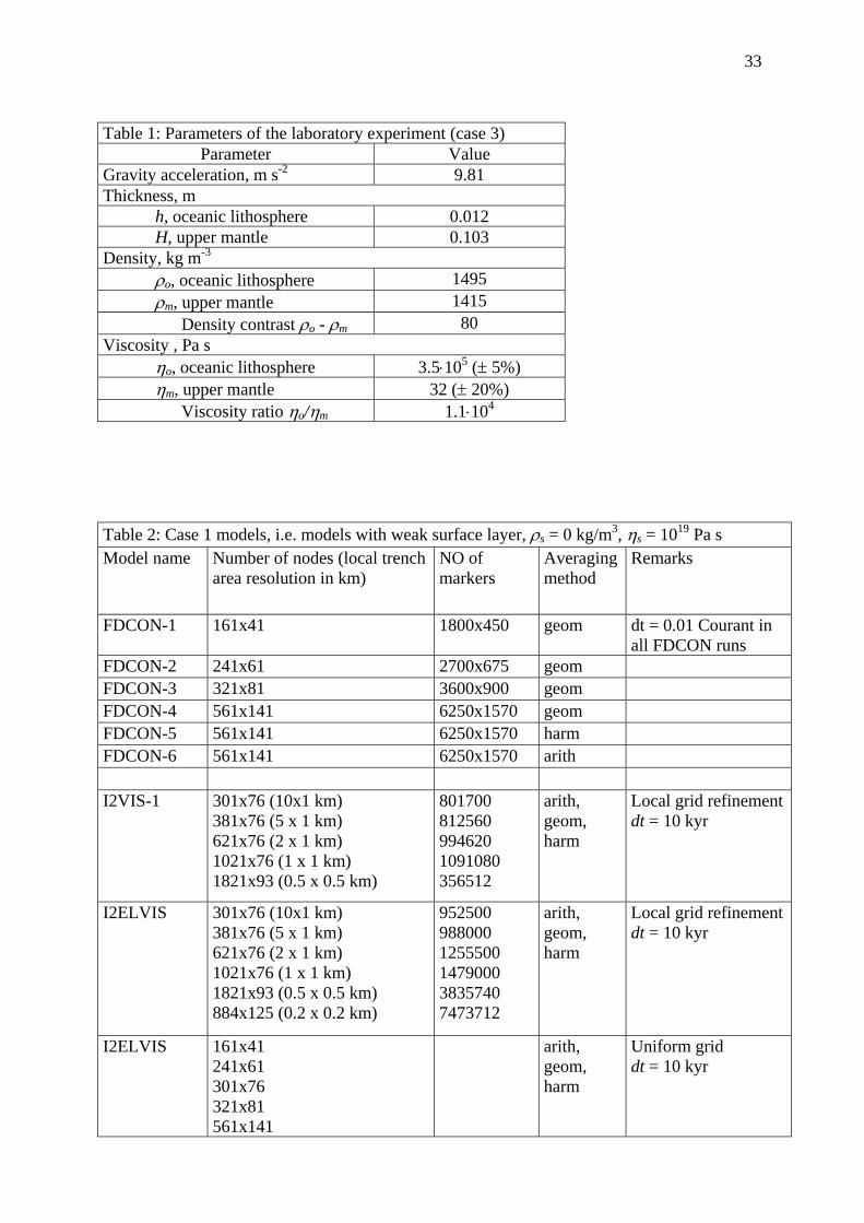
33

Table 1: Parameters of the laboratory experiment (case 3)

Parameter Value Gravity acceleration, m s-2 9.81 Thickness, m

h, oceanic lithosphere 0.012 H, upper mantle 0.103

Density, kg m-3

ρo, oceanic lithosphere 1495 ρm, upper mantle 1415

Density contrast ρo - ρm 80 Viscosity , Pa s

ηo, oceanic lithosphere 3.5⋅105 (± 5%) ηm, upper mantle 32 (± 20%)

Viscosity ratio ηo/ηm 1.1⋅104

Table 2: Case 1 models, i.e. models with weak surface layer, ρs = 0 kg/m3, ηs = 1019 Pa s Model name Number of nodes (local trench

area resolution in km) NO of markers

Averaging method

Remarks

FDCON-1 161x41 1800x450 geom dt = 0.01 Courant in all FDCON runs

FDCON-2 241x61 2700x675 geom FDCON-3 321x81 3600x900 geom FDCON-4 561x141 6250x1570 geom FDCON-5 561x141 6250x1570 harm FDCON-6 561x141 6250x1570 arith I2VIS-1 301x76 (10x1 km)

381x76 (5 x 1 km) 621x76 (2 x 1 km) 1021x76 (1 x 1 km) 1821x93 (0.5 x 0.5 km)

801700 812560 994620 1091080 356512

arith, geom, harm

Local grid refinement dt = 10 kyr

I2ELVIS 301x76 (10x1 km) 381x76 (5 x 1 km) 621x76 (2 x 1 km) 1021x76 (1 x 1 km) 1821x93 (0.5 x 0.5 km) 884x125 (0.2 x 0.2 km)

952500 988000 1255500 1479000 3835740 7473712

arith, geom, harm

Local grid refinement dt = 10 kyr

I2ELVIS 161x41 241x61 301x76 321x81 561x141

arith, geom, harm

Uniform grid dt = 10 kyr

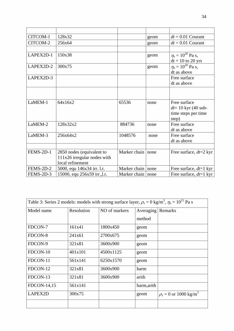
34

CITCOM-1 128x32 geom dt = 0.01 Courant CITCOM-2 256x64 geom dt = 0.01 Courant LAPEX2D-1 150x38 geom ηs = 1020 Pa s,

dt = 10 to 20 yrs LAPEX2D-2 300x75 geom ηs = 1020 Pa s,

dt as above LAPEX2D-3 Free surface

dt as above

LaMEM-1 64x16x2 65536 none Free surface dt= 10 kyr (40 sub-time steps per time step)

LaMEM-2 128x32x2 884736 none

Free surface dt as above

LaMEM-3 256x64x2 1048576 none Free surface dt as above

FEMS-2D-1 2850 nodes (equivalent to

111x26 irregular nodes with local refinement

Marker chain none Free surface, dt=2 kyr

FEMS-2D-2 5000, equ 146x34 irr. l.r. Marker chain none Free surface, dt=1 kyrFEMS-2D-3 15000, equ 256x59 irr.,l.r. Marker chain none Free surface, dt=1 kyr Table 3: Series 2 models: models with strong surface layer, ρs = 0 kg/m3, ηs = 1021 Pa s

Model name Resolution NO of markers Averaging

method

Remarks

FDCON-7 161x41 1800x450 geom

FDCON-8 241x61 2700x675 geom

FDCON-9 321x81 3600x900 geom

FDCON-10 401x101 4500x1125 geom

FDCON-11 561x141 6250x1570 geom

FDCON-12 321x81 3600x900 harm

FDCON-13 321x81 3600x900 arith

FDCON-14,15 561x141 harm,arith

LAPEX2D 300x75 geom ρs = 0 or 1000 kg/m3

35

ABAQUS-mesh 300x70 harm

CITCOM-3 128x32 geom

CITCOM-4 256x64 geom

CITCOM-5 512x128 geom

Fig 1. Model set up and initial condition of the benchmark case 1 and 2.

2

Fig. 2. a) Experimental setup of the subduction benchmark case 3. a = 54 cm, b = 25 cm, l = 40 cm (= 34 cm along surface, 6 cm dipping), w = 25 cm, h = 1.2 cm, H = 10.3 cm. b) Setup for the corresponding numerical models.

3

Fig 3. Typical behaviour of a case 1 model (here FDCON-4 is shown). Streamlines are also shown.

4

Fig 4. Shapes of different case 1 models at similar stages: FDCON: 40 Myr, I2ELVIS: 34.7 Myr, CITCOM: 38.1 Myr. Viscosity averaging: geometric mean in all cases.

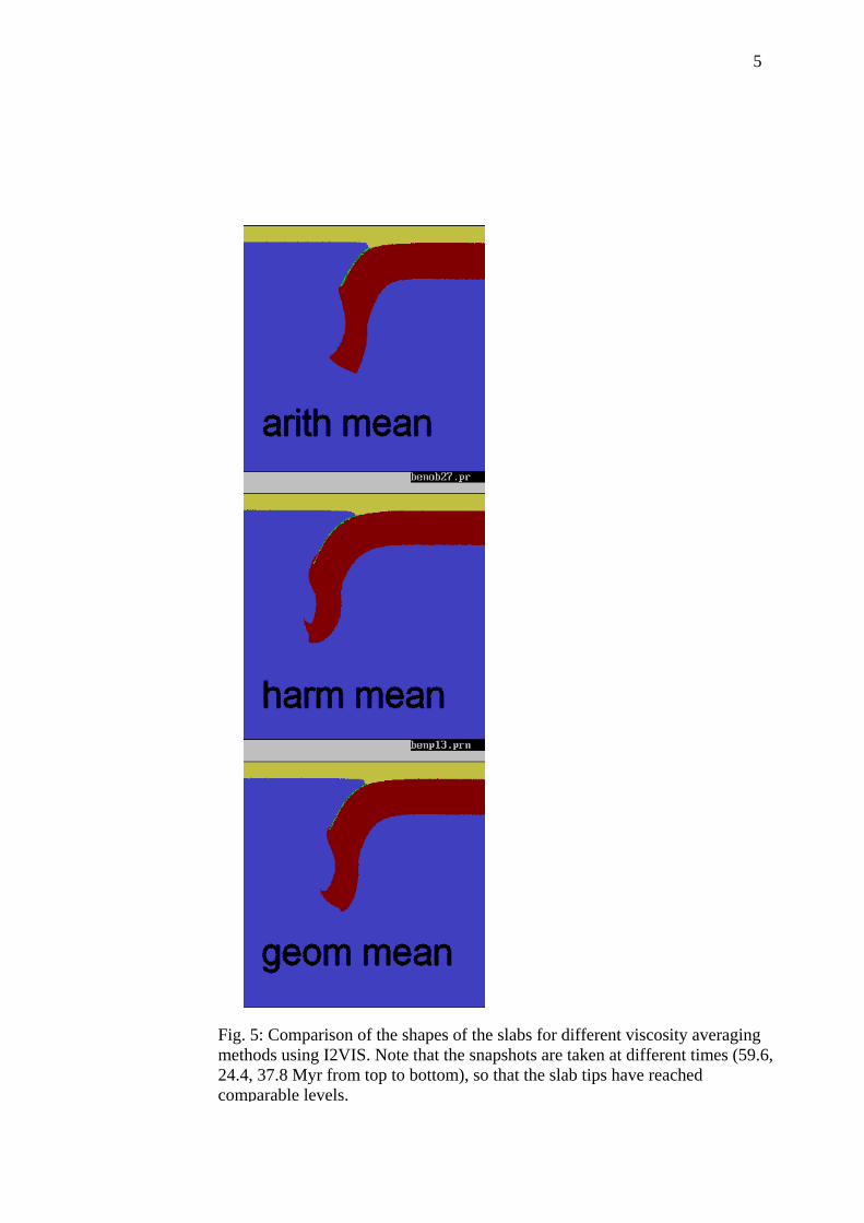
5

Fig. 5: Comparison of the shapes of the slabs for different viscosity averaging methods using I2VIS. Note that the snapshots are taken at different times (59.6, 24.4, 37.8 Myr from top to bottom), so that the slab tips have reached comparable levels.

6

Fig.6. Temporal behaviour of case 1 modelled by different codes with highest resolutions

each. Each curve shows the position of the deepest part of the slab (slab tip) as a function of

time below the initial surface of the lithosphere. See the legends for the used codes and grid

resolution. Note that the codes I2VIS and I2ELVIS also use local refinement at the trench

area (given in parantheses in the legend). Outside the trench area the resolution decreases to

10x46 km at model sides. At the lower boundary the vertical resolution was 1 km. The

rheological means (c.f. section 3.2) are denoted as geom for geometric, harm for harmonic

and arith for arithmetic, repectively. In contrast to the others, LAPEX2D was run with 1020 Pa

s for the weak layer.

7

Fig 7. Resolution test of all models of case 1. The time at which the slab tip passes the 400 km

level beneath the initial lithosphere surface is shown for each model as a function of

characteristic grid size. The different rheological averaging schemes are arithmetic, geometric

and harmonic mean, as well as the infinite norm scheme. While for FDCON, CITCOM, and

I2ELVIS (uniform grid) the characteristic grid size is equal to the actual grid size (equal in

horizontal and vertical direction), the chararcteristic grid size of the I2VIS and I2ELVIS runs

with local refinement was taken as the geometric mean of the nominal grid size (length

divided by number of cells in each direction and then taking the geometric mean of the two

directions) and the finest grid size within trench region (also taking the geometric mean of the

two directions), scaled so that the characteristic grid size equals the nominal grid size for the

coarsest resolution. The non-connected cross symbols show the grid sizes at which the

lithospheric surface coincides with a FD-grid line for FDCON. This sequence correlates with

the oscillations seen in the FDCON –curves.

8

Fig 8. Highest resolution results for trench rollback of case 1 for different rheological

averaging methods (geometric, arithmetic, harmonic mean). Several runs were done with grid

refinement following the moving trench. For these runs, outside the trench area the resolution

decreases to 10x46 km at model sides, except for the 381x76 node model, which has uniform

horizontal resolution with 5x46 km at the model sides. At the lower boundary the vertical

resolution was always 1 km.

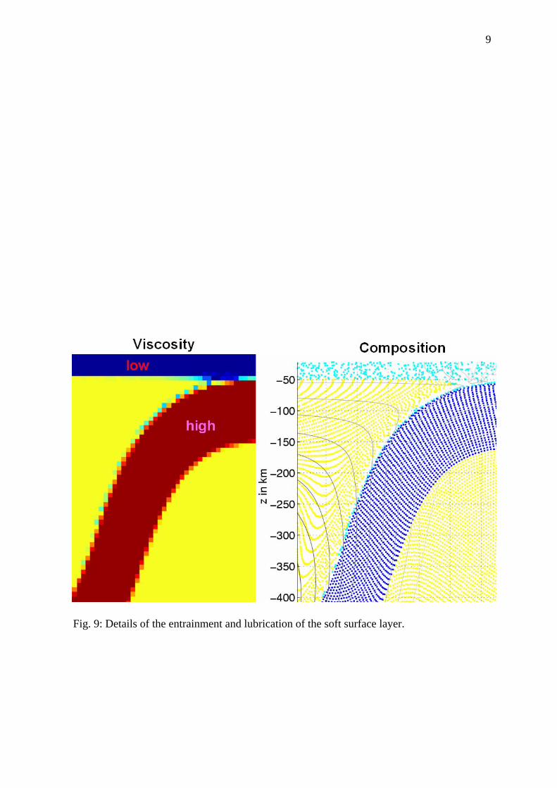
9

Fig. 9: Details of the entrainment and lubrication of the soft surface layer.

10

Fig. 10. Comparison of temporal behaviour of case 1 models assuming a free surface instead

of a weak layer. The FEMS-models used an irregular (irr.) mesh with local refinment (l.r.)

near the trench, the given x-y grid resolution are only approximate values for comparison,

calculated from the total number of nodes. The three FEMS-2D models are very similar so

that the curves partly overlap.

11

Fig. 11. Typical behaviour of a case 2 model (here FDCON-11 is shown)

12

Fig. 12. Shapes of different cased 2 models at similar stages: FDCON: 60 Myr, LAPEX2D at 60Myr, CITCOM at 67.2 Myr. Viscosity averaging: geometric mean in all cases. LAPEX2D used ρs = 1000 kg/m3

13

Fig. 13 Highest resolution results of different codes for slab tip depth evolution for case 2.

Different viscosity averaging schemes (arithmetic, geometric and harmonic means) have been

used.

14

Fig. 14. Result of the laboratory experiment at 6 different times. Note that the dark visibleregions represent the side view of the slab while slightly lighter parts show the central part ofthe slab deeper within the tank.

15

Fig. 15: Surface view of the laboratory model at the time 19' 15'' illustrating the 3D effects.

The brighter part of the plate on the right is still at the surface, the subducted part lies left of

the arcuate trench.

16

Fig. 16. Zoom in for viscosity snapshots of the FEMS2D (left), FDCON (right) numerical modelsfor times 57s, 5' 50'', and 13' 16'' which are comparable to the time steps presented for thelaboratory experiment. For FDCON the harmonic mean for viscosity is used.

17

Fig. 17: a) Comparison between laboratory and numerical slab tip depths obtained by the

codes FDCON, LaMEM and FEMS-2D. FDCON used a viscosity of the soft surface

layer equal to 1/10 of the mantle viscosity b) As a) but for I2ELVIS, using a viscosity of

the soft surface layer of 1/100 of the mantle viscosity

18

Fig. 18: Comparison between experimental and numerical relative slab retreat.

19

Fig. 19. Illustration of the physical meaning of the different averaging methods

20

Fig 20. Effective viscosity of one numerical cell in a Eulerian formulation depending on the fraction of material 2 for the different averaging methods for a viscosity contrast 100 (a) and 10000 (b). c): Depending on the averaging method, the effective

position of the interface is shifted towards the stiff or weak material

21

Fb

ig. 21. a) Resolution test, using FDCON, for a circular body of different density, surrounded y a weak lubrication layer, using the harmonic, arithmetic, geometric or infinite norm mean or viscosity averaging near boundaries. The circular body has a density contrast Δρ with

material, a viscosity 102 times higher then the background viscosity η0 and is situated in the centre of a square box which has a height 10 times the radius r0.

oundary condition at the box sides is free slip. The circular body is surrounded by a of the radius, a viscosity of 10-2 the background viscosity and

as the same density as the background material. The ordinate shows the root-mean-square elocity within the whole box, scaled by Δρ g r0

2/η0. b) Resolution tests for a stiff and weak circular body of different density without lubrication layer (i.e. 2D Stokes flow). Same set up and scalin

frespect to the background

Blubrication layer of thickness 5% hv

g as in a). The stiff cylinder has a viscosity of 100 η B0B, the weak cylinder of 0.01 η B0B.

22

Fig. A1a

Fig. A1b

23

Fig. A1c

Fig. A1d

24

Fig. A1e

Fig. A1 Temporal behaviour of case 1 modelled by different codes and with different

resolution. Each diagram shows the position of the deepest part of the slab (slab tip) as a

function of time below the initial surface of the lithosphere. See the legends for the used codes

and grid resolution. Note that the codes I2VIS and I2ELVIS (a and b) use local refinement at

the trench area (given in parantheses in the legend). Outside the trench area the resolution

decreases to 10x46 km at model sides, except for the 381x76 node model, which has uniform

horizontal resolution with 5x46 km at the model sides. At the lower boundary the vertical

resolution was always 1 km. The rheological means (c.f. section 3.2) are denoted as geom for

eometric, harm for harmonic and arith for arithmetic, repectively. In contrast to the others,

APEX2D (Fig 6e) was run with 1020 Pa s for the weak layer.

g

L

25

Fig A2a

Fig A2b

26

Fig A2c

Fig A2d

Fig A2. Comparison of temporal behaviour of case 1 for models with different rheological

averaging and different resolution. Else as Fig A1.

27

Fig. A3a

Fig. A3b

28

Fig. A3c

Fig A3. Trench rollback of case 1 for different rheological averaging methods using I2ELVIS:

a: geometric mean, b: arithmetic mean, c: harmonic mean. Several runs were done with grid

refinement following the moving trench. In these runs, outside the trench area the resolution

decreases to 10x46 km at model sides, except for the 381x76 node model, which has uniform

horizontal resolution with 5x46 km at the model sides. At the lower boundary the vertical

resolution was always 1 km.

29

Fig. A4a

Fig. A4b

30

Fig. A4c

Fig. A4 Slab tip depth curves for case 2 for different codes and with different resolutions. a)

Resolution test for FDCON and LaMEM models with geometric mean. b) Resolution test for

CITCOM models, one LAPEX2D model added., c) comparison of curves with different

viscosity averaging schemes.

31

Fig. B1. a) Test of case 1 with visco-elastic theology (Youngs modulus 1011 Pa). b) Modification of previous model by adding a highly viscous core in the lithosphere and increasing the Youngs modulus to 1013 Pa