95

TECHNICAL TRANSACTIONS 122018CIVIL ENGINEERING

DOI 1044672353737XCT181869674 SUBMISSION OF THE FINAL VERSION 8112018

Aleksander Urbański orcidorg0000-0002-5544-9134aurbansk123gmailcom orcidorg0000-0003-3283-5005Krzysztof Podleś

Institute of Geotechnics Cracow University of Technology

AbstractThis paper presents an approximate method for a groundwater flow analysis in the case of a slope with vertical dewatering wells distributed equidistantly Firstly a multi-scale problem of flow to a drainage well is solved and flow model to a perforated tube with a filter screen is shown Secondly a method of building quasi-3D flow model of a slope with vertical dewatering wells using a technique of overlapped 2D mesh is shown A short description of the implementation of this 2D3D flow model for the ZSoilPC code is given The results of the described 2D3D method are compared with a referential 3D analysis giving an acceptable level of agreement Finally the 2D3D method of flow analysis is used in a two-phase (flow + deformation) formulation of a slope stability problem The comparison of the results of these analyses with fully 3D (referential) analysis on an example problem provides a very close accurate stability and deformation estimation however the computational time used for the 2D3D analysis is significantly shorter than required by 3D analysisKeywords FEM analysis of groundwater flow slope stability analysis dewatering wells

StreszczeniePrzedstawiono przybliżoną metodę analizy przepływu woacuted gruntowych dla przypadku zbocza ze studniami odwadniającymi rozmieszczonymi w roacutewnych odstępach Na wstępie rozwiązano wieloskalowe zagadnie-nie przepływu do studni odwadniającej i zaprezentowano sposoacuteb budowy zhomogenizowanego modelu filtracji do filtra Następnie zaprezentowano sposoacuteb budowy quasi-3D modelu filtracji w zboczu z pionowy-mi studniami odwadniającymi z wykorzystaniem techniki nakładających się siatek 2D Podano kroacutetki opis implementacji modelu filtracji 2D3D w programie ZSoilPC Wyniki opisanej metody 2D3D poroacutewna-no z referencyjnym modelem 3D dając akceptowalną zgodność Na końcu zastosowano metodę analizy przepływu 2D3D do zagadnień dwufazowych (przepływ + deformacja) dla problemu stateczności zbo-cza Poroacutewnanie wynikoacutew z referencyjną pełną analizą 3D dla przykładowego problemu daje bardzo dobrą ocenę stateczności i deformacji ale czas obliczeniowy używany do analizy 2D3D jest znacznie kroacutetszySłowa kluczowe analiza filtracji MES stateczność zboczy studnie odwadniające

A 2d3d method of the groundwater flow and stability analysis of a slope with dewatering wells

Metoda analizy 2d3d przepływu woacuted gruntowych i stateczności zbocza odwadnianego przy pomocy studni

odwadniających

96

1 Introductory remarks and the motivation

Numerical modelling of groundwater flow performed with use of the finite element method may be presented as a separate problem or as a component of a two-phase (flow + deformation) analysis The first option is often used for the design of water supply (see [6]) or drainage systems The second option is necessary when attempting to investigate the influence of the presence of water within a soil mass which is particularly essential in the context of slope stability problems This concerns both natural and man-made slopes such as an earth dam downstream side slope It is a widely recognised fact that the introduction of drilled dewatering wells lowers the level of the saturated zone which is beneficial for the stability of a structure

An overview of the concerned situation is presented in Fig 1 where vertical dewatering wells with a filtrating zone (screen filter) located on some depth are equidistantly distributed in the longitudinal (Z) direction Even if the filtration properties of the soil are assumed as being constant in the Z-direction (while they may vary in the XY cross section plane) the problem of flow is three-dimensional but submitted to periodicity constraints In a recent practice 3D flow problem set in the domain of one segment (with Z-length a) between drainage wells may be solved within an acceptably short timeframe thus for flow analysis exclusively there would not be a requirement for an approximate method However this is not the case of slope stability analysis basing on two-phase (flow + deformation) formulation and Terzagi-Bishop principle Modelling a continuum with a 3D field of water pressure would require full 3D fields of stresses and what follows strains and displacements even in the case when the plane strain (PS) assumptions are commonly accepted like while performing stability analysis of man-made slopes Plane strain assumptions are in considered case violated 3D stability analyses performed with use of the c-f reduction method which might be formulated as well require considerably more time and computational power than 2D analysis ndash see the comparison in the example given in section 6 It is worth noting that with these types of problems dense meshing in zones where strain localisation is expected (which are a-priori unknown) is necessary

Fig 1 An overview of a slope with dewatering wells free surfaces 1) at the section coming through vertical well 2) at the section in the mid-distance

97

The main objective of this article is to perform the analysis of dewatered slopes in the 2D domain of its cross-section with plane strain assumption and water pressure field being an averaged of these in Z-direction The developed method is based on an approximate solution of the groundwater flow problem on overlapped meshes describing flow through the slope and flow to the draining wells An implementation done in custom version of ZSoilPC code allows to show the robustness and acceptable engineering accuracy of the developed 2D3D method

2 Flow to a drainage well as a multi-scale problem

The first task to be solved is to develop a proper model of seepage to a filter screen in order to estimate its efficiency This can be achieved empirically based on in situ or laboratory testing which is beyond the scope of this paper or numerically with the use of the micro-level analysis of flow and the homogenisation technique presented below The validity of Darcyrsquos law with full saturation condition is assumed A gravity term in Darcyrsquos law is neglected while performing the described micro-level analysis

The scale of the geometry of the openings in the filter screen tube is within the range of 10-3 m the scale of macro-level characteristic dimensions may reach 101 m In these circumstances the need for a multi-scale analysis is evident as it is extremely difficult to build a single model dealing with the flow within the vicinity of the drain tube (scale mm) and at a large distance from it Scale separation leads to multi-scale analysis which consists of two problems concerning

micro level ndash set in the 3D domain of periodic cell resulting from the geometry of the filter screen This analysis is used to establish fluxes q for the given pressure head p see Fig 2b

macro level ndash referring to the whole system (2D or 3D) with well modelled as a tube (diameter D thickness D) and permeability coefficient set by equivalence of flow with these established during micro level analysis

Fig 2 Multi-scale analysis based on the homogenisation of the flow

98

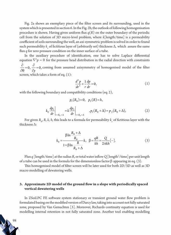
Fig 2a shows an exemplary piece of the filter screen and its surrounding used in the system which is presented in section 6 In the Fig 2b the outlook of following homogenisation procedure is shown Having given uniform flux q(R) on the outer boundary of the periodic cell from the solution of 3D micro-level problem where k[lengthtime] is a permeability coefficient of soils surrounding the well an axi-symmetric problem is solved in order to found such permeability ko of fictitious layer of (arbitrarily set) thickness D which assure the same flux q for zero pressure condition on the inner surface of a tube

In the auxiliary procedure of identification one has to solve Laplace differential equation nabla2p = 0 for the pressure head distribution in the radial direction with constraints

0 0

ycoming from assumed axisymmetry of homogenised model of the filter

screen which takes a form of eq (1)

d pdr r

dpdr

2

21

0 (1)

with the following boundary and compatibility conditions (eq 2)

p R p R h1 0 20( ) ( ) = =

kdpdr

kdpdr

p R p Rr R r R

01 2

1 0 2 00 0

( ) ( ) (2)

For given R0 R k h this leads to a formula for permeability ko of fictitious layer with the thickness D

k

RR

RR

kqRkh

Qkh0

0

0

0

1 2

ln

ln [ ]

(3)

Flux q [lengthtime] at the radius R or total water inflow Q [length2time] per unit length of a tube can be used in the formula for the dimensionless factor b appearing in eq (3)

This homogenised model of filter screen will be later used for both 2D3D as well as 3D macro modelling of dewatering wells

3 Approximate 2D model of the ground flow in a slope with periodically spaced vertical dewatering wells

In ZSoilPC FE software system stationary or transient ground water flow problem is formulated basing on the modified version of Darcy law taking into account not fully saturated zone proposed by Van Genuchten [3] Moreover Richards continuity equation is used for modelling internal retention in not fully saturated zone Another tool enabling modelling

99

without any user intervention in computation consists of seepage elements automatically switching boundary condition from fully free flow to no-flow depending on the pressure at the boundary For details see [2 4 5] All mentioned features are active in the present issue

The idea is to decompose flow field in the dewatered slope at following parts flow along the slope for which base 2D FE mesh describing geometry of the slope

cross-section is built preserving its permeability properties k(X Y) and boundary conditions

flow towards the well performed on a set of overlapped FE meshes applied in the well influence zone size of which is related to the distance of wells (= 2a) in Z direction (see the Fig 3) Each of them represents a sector of 3D system Permeability of materials set in this fictitious media inherits permeability k(X Y) from the base mesh but those are finally modified on the principle of geometrical equivalence assuming radial flow direction with the centre at the well The equivalence must take into consideration a fact that plane flow is set for unit thickness g = 10 [length] of the model in perpendicular direction On the length of filter screen the tube of diameter D is surrounded by fictitious layer with permeability coming from ko of homogenised model and current sectorial geometry Outside the filter screen on the tube inner surface a no-flow condition qn = 0 is set Additionally on the limits of the well influence zone the condition of equal pressures with base mesh is set by introducing penalty permeability kinfin (ie equal to a very large value) at the ldquoarmsrdquo perpendicular to the base mesh

It is worth noting that in a given FE software building a FE model with overlapped meshes must be allowed like it is in ZSoilPC

Fig 3 Details of the equivalent 2D3D flow model

Number of radii m is set by the user as well as the number of circles n The permeability at the ij position considering geometry equals

k k x yA

aijij ( ) (4)

where Aij is averaged width attached to i-th zone at j-th sector of the radial mesh For regular shape they are given in eq 5 for the remaining they can be derived analogously

100

F R R AF

R RR R

ij i ij

ijij

i i

i ij

( ) 1

2 2

1

1

2 2

(5)

where Fij is an areaIn a custom version of ZSoilPC code process of building any model as described above

is fully automatized and after creating the base 2D FE mesh the user needs to provide only minimal amount of data describing geometry of wells additional discretization permeability ko and thickness D of fictitious layer of homogenised well model according to p 2 There may be a few wells modelled at single base mesh with one objection ie that their influence zones do not overlap

User interface for wells definition is presented in the Fig 4

Fig 4 User interface for wells definition

4 Comparison of results between 2D3D against 3D flow modelling

The first test example is based on comparison of a result for steady-state flow analysis obtained for full 3D model with results for equivalent 2D3D model Draft of the geometry with resulting base FE mesh is presented in Fig 5 Parameters presented in Fig 5a were used to generate mesh for 2D3D model FE meshes with fluid boundary conditions for 2D3D method and 3D model are shown in Fig 6a and 6b respectively Permeability coefficient is k = 1 md for whole domain despite zone of the filter screen (D = 028 m) where homogenised model is applied with ko = 0231 md at the fictitious layer of thickness D = 006 m

101

Fig 5 Geometry of the test model and resulting base FE mesh

Fig 6 FE meshes with fluid boundary conditions for a) 2D3D model b) referential 3D model

Fig 7 Fluid velocities distribution in cross sections for a) 2D3D model b) referential 3D model

In order to compare total flow to the dewatering well for both models the integrals of a fluid velocities through cross sections defined on left and right boundary sides are calculated Fluid velocities distribution in cross sections with resultant integrals for 2D3D model and 3D model are shown in Fig 7a and 7b The assumed distance between wells is 2a=12m

Total flow to dewatering well for 2D3D model equals

Q Q Q am

d mm

d mmD2

3 3

1 2 3 87 2 07 6 1

( ) 00 79

3

md

(6)

a) b)

a) b)

102

Total flow to dewatering well for 3D model equals

Q Q Qmd

md

mD D D3 3 3

3 3

1 2 18 53 8 13 10 40

33

d

(7)

Difference is

e

10 79 10 4010 40

3 75 (8)

The comparison of the pore pressure distribution for 2D3D model and referential 3D model is shown in Fig 8 Differences for both models in total flow to dewatering well (less than 4) and pore pressure distribution are acceptable for engineering applications Data preparation is much simpler for 2D3D model with automatic well generation than for 3D model for which all details of the well and fine mesh around well have to be generated manually Additionally mesh generation when a well position is changed is created automatically for 2D3D model The 3D model has to be created nearly from the beginning

Fig 8 Pore pressure distribution for a) 2D3D model b) referential 3D model (in the mid-section)

a) b)

5 Application of the 2D3D method to two-phase (deformation + flow) analysis

The two-phase analysis for 2D3D model requires special treatment for material properties and boundary conditions Deformation + flow analysis is performed on 2D base mesh when perpendicular or radial ldquoarmsrdquo have influence on flow analysis only Young modulus is assumed to be close to zero and displacement degrees of freedom are fixed everywhere in the domain of perpendicular ldquoarmrdquo in order to neglect its influence on mechanical analysis This sub-model has pressure degrees of freedom only Meshes of the base model and ldquoarmsrdquo can be inconsistent Continuity of pressure fields between both sub-models is preserved by

103

means of nodal link option available in ZSoilPC Such schema of partial separation of flow and deformation+flow sub-models is presented in Fig 9

Fig 9 Partial separation of flow and deformation+flow sub-models for two-phase analysis

6 Application of developed method of flow analysis to the slope stability problem

The effectiveness of 2D3D model compared with full 3D model is presented on an example of slope stability problem The analysis of pore pressure distribution influences on results of slope stability was performed by Finite Element and c-f reduction method using ZSoilPCreg code The applied c-f reduction method was firstly introduced into the early version of ZSoilPC code (circa 1985) its details may be found in ZSoil documentation [8] More examples of usage of this method in landslide stability analyses can be found in Truty et al [2] Zheng et al [7] Ozbay and Cabalar [1] The soil continuum was treated as an elastic-plastic one with Mohr-Coulomb yield condition The influence of an underground water pressure field in saturated or partially saturated zone was taken into account with enhancements of the flow theory given in Van Genuchten [3] basing on observed water table

The geometry of the analysed problem with resulting base FE mesh are presented in Fig 10 and parameters for mesh generation are shown in Fig 11 FE meshes with fluid boundary conditions for 2D3D method and 3D model are shown in Fig 12 and Fig 13 respectively

Fig 10 The geometry of the test model and resulting base FE mesh

104

Fig 11 The geometry of the wells and parameters for mesh generation

Fig 12 FE mesh with boundary conditions for 2D3D model

Fig 13 FE mesh with boundary conditions for referential 3D model

105

Fig 14 Distribution of total displacements on deformed mesh for 2D3D model for safety factor SF2D3D = 1519

Fig 15 Distribution of total displacements on deformed mesh for referential 3D model for safety factor SF3D = 1509

In the analysis following strength and permeability parameters were assumed material 1 c1 = 30 kPa j1 = 30deg k1 = 00416 md (sand) material 2 c2 = 200 kPa j2 = 30deg k2 = 00000416 md (clay)

The results of stability analysis are presented in Fig 14 and 15 It is worth to mention that almost identical deformation (failure pattern) appears in both approaches The computed safety factors are very close one to another as well For 2D3D model it equals SF2D3D = 1519 and for referential 3D model SF3D = 1509 It is worth mentioning that elapsed time of computations differs substantially as the analysis for 2D3D model was performed in 10 minutes while for 3D model it takes 10 hours ie ~60 times more for the same mesh density in XY plane

106

7 Conclusions

The presented approximate method of an analysis of the groundwater flow in a slope with vertical dewatering wells distributed periodically proves to be an efficient tool for engineering problems requiring spatial distribution of the water pressure field

The main gain is that analysis can be set in 2D domain instead of 3D modelling leading to practically very close results remaining within the 5 margin of error It concerns deformation and stability assessment in case of two-phase analysis as well as inflow to the wells

The presented method allows to obtain results in a rapid way In case of problems with assessment of stability in existing structure it may be useful tool for prediction of its behaviour in varying condition In a design process it may serve as a tool to optimize dewatering system in terms of location of the wells or applied drainage capability

References

[1] Ozbay A Cabalar AF FEM and LEM stability analyses of the fatal landslides at Ccediloumlllolar open-cast lignite mine in Elbistan Turkey ldquoLandslidesrdquo 122015 155ndash163

[2] Truty A Urbański A Grodecki M Podleś K Computer aided models of landslides and their protection problems ldquoScientific-Technical Papers of Communication Engineers and Technicians of the Republic of Polandrdquo in Krakow No 88 issue 88 (144)2009 395ndash419

[3] Van Genuchten MTh A closed form equation for predicting the hydraulic conductivity of unsaturated soils ldquoSoil Science Society of America Journalrdquo 441980 892ndash898

[4] Urbański A Grodecki M Kot A Numerical simulations in analysis of anti-flood ambankmentsrdquoJournal of Civil Engineering Environment and Architecturerdquo 2016

[5] Urbański A Grodecki M FE Approach to coupled transient flow and stability analysis of anti-flood ambankments ldquo3-rd Int Conference on Advances of Computer Methods in Geotechnical and Geo-environmental Engineeringrdquo Moscow 2000

[6] Wilk BK Urbański A The impact of the shape of screen openings on groundwater flow to a deep drilled well ldquoTechnical Transactionsrdquo 112018 to appear

[7] Zheng Y Tang X Zhao S Deng C Lei W3 Strength reduction and step-loading finite element approaches in geotechnical engineering ldquoJournal of Rock Mechanics and Geotechnical Engineeringrdquo 1(1)2009 21ndash30

[8] Zimmemann Th Truty A Urbański A Podleś K Z_SoilPC 2003 manual Theory Elmepress international amp Zace Services ltd Lausanne Switzerland 2005

If you want to quote this article its proper bibliographic entry is as follow Urbański A Podleś K A 2D3D method of the groundwater flow and stability analysis of a slope with dewatering wells Technical Transactions Vol 122018 pp 95ndash106

97

The main objective of this article is to perform the analysis of dewatered slopes in the 2D domain of its cross-section with plane strain assumption and water pressure field being an averaged of these in Z-direction The developed method is based on an approximate solution of the groundwater flow problem on overlapped meshes describing flow through the slope and flow to the draining wells An implementation done in custom version of ZSoilPC code allows to show the robustness and acceptable engineering accuracy of the developed 2D3D method

2 Flow to a drainage well as a multi-scale problem

The first task to be solved is to develop a proper model of seepage to a filter screen in order to estimate its efficiency This can be achieved empirically based on in situ or laboratory testing which is beyond the scope of this paper or numerically with the use of the micro-level analysis of flow and the homogenisation technique presented below The validity of Darcyrsquos law with full saturation condition is assumed A gravity term in Darcyrsquos law is neglected while performing the described micro-level analysis

The scale of the geometry of the openings in the filter screen tube is within the range of 10-3 m the scale of macro-level characteristic dimensions may reach 101 m In these circumstances the need for a multi-scale analysis is evident as it is extremely difficult to build a single model dealing with the flow within the vicinity of the drain tube (scale mm) and at a large distance from it Scale separation leads to multi-scale analysis which consists of two problems concerning

micro level ndash set in the 3D domain of periodic cell resulting from the geometry of the filter screen This analysis is used to establish fluxes q for the given pressure head p see Fig 2b

macro level ndash referring to the whole system (2D or 3D) with well modelled as a tube (diameter D thickness D) and permeability coefficient set by equivalence of flow with these established during micro level analysis

Fig 2 Multi-scale analysis based on the homogenisation of the flow

98

Fig 2a shows an exemplary piece of the filter screen and its surrounding used in the system which is presented in section 6 In the Fig 2b the outlook of following homogenisation procedure is shown Having given uniform flux q(R) on the outer boundary of the periodic cell from the solution of 3D micro-level problem where k[lengthtime] is a permeability coefficient of soils surrounding the well an axi-symmetric problem is solved in order to found such permeability ko of fictitious layer of (arbitrarily set) thickness D which assure the same flux q for zero pressure condition on the inner surface of a tube

In the auxiliary procedure of identification one has to solve Laplace differential equation nabla2p = 0 for the pressure head distribution in the radial direction with constraints

0 0

ycoming from assumed axisymmetry of homogenised model of the filter

screen which takes a form of eq (1)

d pdr r

dpdr

2

21

0 (1)

with the following boundary and compatibility conditions (eq 2)

p R p R h1 0 20( ) ( ) = =

kdpdr

kdpdr

p R p Rr R r R

01 2

1 0 2 00 0

( ) ( ) (2)

For given R0 R k h this leads to a formula for permeability ko of fictitious layer with the thickness D

k

RR

RR

kqRkh

Qkh0

0

0

0

1 2

ln

ln [ ]

(3)

Flux q [lengthtime] at the radius R or total water inflow Q [length2time] per unit length of a tube can be used in the formula for the dimensionless factor b appearing in eq (3)

This homogenised model of filter screen will be later used for both 2D3D as well as 3D macro modelling of dewatering wells

3 Approximate 2D model of the ground flow in a slope with periodically spaced vertical dewatering wells

In ZSoilPC FE software system stationary or transient ground water flow problem is formulated basing on the modified version of Darcy law taking into account not fully saturated zone proposed by Van Genuchten [3] Moreover Richards continuity equation is used for modelling internal retention in not fully saturated zone Another tool enabling modelling

99

without any user intervention in computation consists of seepage elements automatically switching boundary condition from fully free flow to no-flow depending on the pressure at the boundary For details see [2 4 5] All mentioned features are active in the present issue

The idea is to decompose flow field in the dewatered slope at following parts flow along the slope for which base 2D FE mesh describing geometry of the slope

cross-section is built preserving its permeability properties k(X Y) and boundary conditions

flow towards the well performed on a set of overlapped FE meshes applied in the well influence zone size of which is related to the distance of wells (= 2a) in Z direction (see the Fig 3) Each of them represents a sector of 3D system Permeability of materials set in this fictitious media inherits permeability k(X Y) from the base mesh but those are finally modified on the principle of geometrical equivalence assuming radial flow direction with the centre at the well The equivalence must take into consideration a fact that plane flow is set for unit thickness g = 10 [length] of the model in perpendicular direction On the length of filter screen the tube of diameter D is surrounded by fictitious layer with permeability coming from ko of homogenised model and current sectorial geometry Outside the filter screen on the tube inner surface a no-flow condition qn = 0 is set Additionally on the limits of the well influence zone the condition of equal pressures with base mesh is set by introducing penalty permeability kinfin (ie equal to a very large value) at the ldquoarmsrdquo perpendicular to the base mesh

It is worth noting that in a given FE software building a FE model with overlapped meshes must be allowed like it is in ZSoilPC

Fig 3 Details of the equivalent 2D3D flow model

Number of radii m is set by the user as well as the number of circles n The permeability at the ij position considering geometry equals

k k x yA

aijij ( ) (4)

where Aij is averaged width attached to i-th zone at j-th sector of the radial mesh For regular shape they are given in eq 5 for the remaining they can be derived analogously

100

F R R AF

R RR R

ij i ij

ijij

i i

i ij

( ) 1

2 2

1

1

2 2

(5)

where Fij is an areaIn a custom version of ZSoilPC code process of building any model as described above

is fully automatized and after creating the base 2D FE mesh the user needs to provide only minimal amount of data describing geometry of wells additional discretization permeability ko and thickness D of fictitious layer of homogenised well model according to p 2 There may be a few wells modelled at single base mesh with one objection ie that their influence zones do not overlap

User interface for wells definition is presented in the Fig 4

Fig 4 User interface for wells definition

4 Comparison of results between 2D3D against 3D flow modelling

The first test example is based on comparison of a result for steady-state flow analysis obtained for full 3D model with results for equivalent 2D3D model Draft of the geometry with resulting base FE mesh is presented in Fig 5 Parameters presented in Fig 5a were used to generate mesh for 2D3D model FE meshes with fluid boundary conditions for 2D3D method and 3D model are shown in Fig 6a and 6b respectively Permeability coefficient is k = 1 md for whole domain despite zone of the filter screen (D = 028 m) where homogenised model is applied with ko = 0231 md at the fictitious layer of thickness D = 006 m

101

Fig 5 Geometry of the test model and resulting base FE mesh

Fig 6 FE meshes with fluid boundary conditions for a) 2D3D model b) referential 3D model

Fig 7 Fluid velocities distribution in cross sections for a) 2D3D model b) referential 3D model

In order to compare total flow to the dewatering well for both models the integrals of a fluid velocities through cross sections defined on left and right boundary sides are calculated Fluid velocities distribution in cross sections with resultant integrals for 2D3D model and 3D model are shown in Fig 7a and 7b The assumed distance between wells is 2a=12m

Total flow to dewatering well for 2D3D model equals

Q Q Q am

d mm

d mmD2

3 3

1 2 3 87 2 07 6 1

( ) 00 79

3

md

(6)

a) b)

a) b)

102

Total flow to dewatering well for 3D model equals

Q Q Qmd

md

mD D D3 3 3

3 3

1 2 18 53 8 13 10 40

33

d

(7)

Difference is

e

10 79 10 4010 40

3 75 (8)

The comparison of the pore pressure distribution for 2D3D model and referential 3D model is shown in Fig 8 Differences for both models in total flow to dewatering well (less than 4) and pore pressure distribution are acceptable for engineering applications Data preparation is much simpler for 2D3D model with automatic well generation than for 3D model for which all details of the well and fine mesh around well have to be generated manually Additionally mesh generation when a well position is changed is created automatically for 2D3D model The 3D model has to be created nearly from the beginning

Fig 8 Pore pressure distribution for a) 2D3D model b) referential 3D model (in the mid-section)

a) b)

5 Application of the 2D3D method to two-phase (deformation + flow) analysis

The two-phase analysis for 2D3D model requires special treatment for material properties and boundary conditions Deformation + flow analysis is performed on 2D base mesh when perpendicular or radial ldquoarmsrdquo have influence on flow analysis only Young modulus is assumed to be close to zero and displacement degrees of freedom are fixed everywhere in the domain of perpendicular ldquoarmrdquo in order to neglect its influence on mechanical analysis This sub-model has pressure degrees of freedom only Meshes of the base model and ldquoarmsrdquo can be inconsistent Continuity of pressure fields between both sub-models is preserved by

103

means of nodal link option available in ZSoilPC Such schema of partial separation of flow and deformation+flow sub-models is presented in Fig 9

Fig 9 Partial separation of flow and deformation+flow sub-models for two-phase analysis

6 Application of developed method of flow analysis to the slope stability problem

The effectiveness of 2D3D model compared with full 3D model is presented on an example of slope stability problem The analysis of pore pressure distribution influences on results of slope stability was performed by Finite Element and c-f reduction method using ZSoilPCreg code The applied c-f reduction method was firstly introduced into the early version of ZSoilPC code (circa 1985) its details may be found in ZSoil documentation [8] More examples of usage of this method in landslide stability analyses can be found in Truty et al [2] Zheng et al [7] Ozbay and Cabalar [1] The soil continuum was treated as an elastic-plastic one with Mohr-Coulomb yield condition The influence of an underground water pressure field in saturated or partially saturated zone was taken into account with enhancements of the flow theory given in Van Genuchten [3] basing on observed water table

The geometry of the analysed problem with resulting base FE mesh are presented in Fig 10 and parameters for mesh generation are shown in Fig 11 FE meshes with fluid boundary conditions for 2D3D method and 3D model are shown in Fig 12 and Fig 13 respectively

Fig 10 The geometry of the test model and resulting base FE mesh

104

Fig 11 The geometry of the wells and parameters for mesh generation

Fig 12 FE mesh with boundary conditions for 2D3D model

Fig 13 FE mesh with boundary conditions for referential 3D model

105

Fig 14 Distribution of total displacements on deformed mesh for 2D3D model for safety factor SF2D3D = 1519

Fig 15 Distribution of total displacements on deformed mesh for referential 3D model for safety factor SF3D = 1509

In the analysis following strength and permeability parameters were assumed material 1 c1 = 30 kPa j1 = 30deg k1 = 00416 md (sand) material 2 c2 = 200 kPa j2 = 30deg k2 = 00000416 md (clay)

The results of stability analysis are presented in Fig 14 and 15 It is worth to mention that almost identical deformation (failure pattern) appears in both approaches The computed safety factors are very close one to another as well For 2D3D model it equals SF2D3D = 1519 and for referential 3D model SF3D = 1509 It is worth mentioning that elapsed time of computations differs substantially as the analysis for 2D3D model was performed in 10 minutes while for 3D model it takes 10 hours ie ~60 times more for the same mesh density in XY plane

106

7 Conclusions

The presented approximate method of an analysis of the groundwater flow in a slope with vertical dewatering wells distributed periodically proves to be an efficient tool for engineering problems requiring spatial distribution of the water pressure field

The main gain is that analysis can be set in 2D domain instead of 3D modelling leading to practically very close results remaining within the 5 margin of error It concerns deformation and stability assessment in case of two-phase analysis as well as inflow to the wells

The presented method allows to obtain results in a rapid way In case of problems with assessment of stability in existing structure it may be useful tool for prediction of its behaviour in varying condition In a design process it may serve as a tool to optimize dewatering system in terms of location of the wells or applied drainage capability

References

[1] Ozbay A Cabalar AF FEM and LEM stability analyses of the fatal landslides at Ccediloumlllolar open-cast lignite mine in Elbistan Turkey ldquoLandslidesrdquo 122015 155ndash163

[2] Truty A Urbański A Grodecki M Podleś K Computer aided models of landslides and their protection problems ldquoScientific-Technical Papers of Communication Engineers and Technicians of the Republic of Polandrdquo in Krakow No 88 issue 88 (144)2009 395ndash419

[3] Van Genuchten MTh A closed form equation for predicting the hydraulic conductivity of unsaturated soils ldquoSoil Science Society of America Journalrdquo 441980 892ndash898

[4] Urbański A Grodecki M Kot A Numerical simulations in analysis of anti-flood ambankmentsrdquoJournal of Civil Engineering Environment and Architecturerdquo 2016

[5] Urbański A Grodecki M FE Approach to coupled transient flow and stability analysis of anti-flood ambankments ldquo3-rd Int Conference on Advances of Computer Methods in Geotechnical and Geo-environmental Engineeringrdquo Moscow 2000

[6] Wilk BK Urbański A The impact of the shape of screen openings on groundwater flow to a deep drilled well ldquoTechnical Transactionsrdquo 112018 to appear

[7] Zheng Y Tang X Zhao S Deng C Lei W3 Strength reduction and step-loading finite element approaches in geotechnical engineering ldquoJournal of Rock Mechanics and Geotechnical Engineeringrdquo 1(1)2009 21ndash30

[8] Zimmemann Th Truty A Urbański A Podleś K Z_SoilPC 2003 manual Theory Elmepress international amp Zace Services ltd Lausanne Switzerland 2005

If you want to quote this article its proper bibliographic entry is as follow Urbański A Podleś K A 2D3D method of the groundwater flow and stability analysis of a slope with dewatering wells Technical Transactions Vol 122018 pp 95ndash106

98

Fig 2a shows an exemplary piece of the filter screen and its surrounding used in the system which is presented in section 6 In the Fig 2b the outlook of following homogenisation procedure is shown Having given uniform flux q(R) on the outer boundary of the periodic cell from the solution of 3D micro-level problem where k[lengthtime] is a permeability coefficient of soils surrounding the well an axi-symmetric problem is solved in order to found such permeability ko of fictitious layer of (arbitrarily set) thickness D which assure the same flux q for zero pressure condition on the inner surface of a tube

In the auxiliary procedure of identification one has to solve Laplace differential equation nabla2p = 0 for the pressure head distribution in the radial direction with constraints

0 0

ycoming from assumed axisymmetry of homogenised model of the filter

screen which takes a form of eq (1)

d pdr r

dpdr

2

21

0 (1)

with the following boundary and compatibility conditions (eq 2)

p R p R h1 0 20( ) ( ) = =

kdpdr

kdpdr

p R p Rr R r R

01 2

1 0 2 00 0

( ) ( ) (2)

For given R0 R k h this leads to a formula for permeability ko of fictitious layer with the thickness D

k

RR

RR

kqRkh

Qkh0

0

0

0

1 2

ln

ln [ ]

(3)

Flux q [lengthtime] at the radius R or total water inflow Q [length2time] per unit length of a tube can be used in the formula for the dimensionless factor b appearing in eq (3)

This homogenised model of filter screen will be later used for both 2D3D as well as 3D macro modelling of dewatering wells

3 Approximate 2D model of the ground flow in a slope with periodically spaced vertical dewatering wells

In ZSoilPC FE software system stationary or transient ground water flow problem is formulated basing on the modified version of Darcy law taking into account not fully saturated zone proposed by Van Genuchten [3] Moreover Richards continuity equation is used for modelling internal retention in not fully saturated zone Another tool enabling modelling

99

without any user intervention in computation consists of seepage elements automatically switching boundary condition from fully free flow to no-flow depending on the pressure at the boundary For details see [2 4 5] All mentioned features are active in the present issue

The idea is to decompose flow field in the dewatered slope at following parts flow along the slope for which base 2D FE mesh describing geometry of the slope

cross-section is built preserving its permeability properties k(X Y) and boundary conditions

flow towards the well performed on a set of overlapped FE meshes applied in the well influence zone size of which is related to the distance of wells (= 2a) in Z direction (see the Fig 3) Each of them represents a sector of 3D system Permeability of materials set in this fictitious media inherits permeability k(X Y) from the base mesh but those are finally modified on the principle of geometrical equivalence assuming radial flow direction with the centre at the well The equivalence must take into consideration a fact that plane flow is set for unit thickness g = 10 [length] of the model in perpendicular direction On the length of filter screen the tube of diameter D is surrounded by fictitious layer with permeability coming from ko of homogenised model and current sectorial geometry Outside the filter screen on the tube inner surface a no-flow condition qn = 0 is set Additionally on the limits of the well influence zone the condition of equal pressures with base mesh is set by introducing penalty permeability kinfin (ie equal to a very large value) at the ldquoarmsrdquo perpendicular to the base mesh

It is worth noting that in a given FE software building a FE model with overlapped meshes must be allowed like it is in ZSoilPC

Fig 3 Details of the equivalent 2D3D flow model

Number of radii m is set by the user as well as the number of circles n The permeability at the ij position considering geometry equals

k k x yA

aijij ( ) (4)

where Aij is averaged width attached to i-th zone at j-th sector of the radial mesh For regular shape they are given in eq 5 for the remaining they can be derived analogously

100

F R R AF

R RR R

ij i ij

ijij

i i

i ij

( ) 1

2 2

1

1

2 2

(5)

where Fij is an areaIn a custom version of ZSoilPC code process of building any model as described above

is fully automatized and after creating the base 2D FE mesh the user needs to provide only minimal amount of data describing geometry of wells additional discretization permeability ko and thickness D of fictitious layer of homogenised well model according to p 2 There may be a few wells modelled at single base mesh with one objection ie that their influence zones do not overlap

User interface for wells definition is presented in the Fig 4

Fig 4 User interface for wells definition

4 Comparison of results between 2D3D against 3D flow modelling

The first test example is based on comparison of a result for steady-state flow analysis obtained for full 3D model with results for equivalent 2D3D model Draft of the geometry with resulting base FE mesh is presented in Fig 5 Parameters presented in Fig 5a were used to generate mesh for 2D3D model FE meshes with fluid boundary conditions for 2D3D method and 3D model are shown in Fig 6a and 6b respectively Permeability coefficient is k = 1 md for whole domain despite zone of the filter screen (D = 028 m) where homogenised model is applied with ko = 0231 md at the fictitious layer of thickness D = 006 m

101

Fig 5 Geometry of the test model and resulting base FE mesh

Fig 6 FE meshes with fluid boundary conditions for a) 2D3D model b) referential 3D model

Fig 7 Fluid velocities distribution in cross sections for a) 2D3D model b) referential 3D model

In order to compare total flow to the dewatering well for both models the integrals of a fluid velocities through cross sections defined on left and right boundary sides are calculated Fluid velocities distribution in cross sections with resultant integrals for 2D3D model and 3D model are shown in Fig 7a and 7b The assumed distance between wells is 2a=12m

Total flow to dewatering well for 2D3D model equals

Q Q Q am

d mm

d mmD2

3 3

1 2 3 87 2 07 6 1

( ) 00 79

3

md

(6)

a) b)

a) b)

102

Total flow to dewatering well for 3D model equals

Q Q Qmd

md

mD D D3 3 3

3 3

1 2 18 53 8 13 10 40

33

d

(7)

Difference is

e

10 79 10 4010 40

3 75 (8)

The comparison of the pore pressure distribution for 2D3D model and referential 3D model is shown in Fig 8 Differences for both models in total flow to dewatering well (less than 4) and pore pressure distribution are acceptable for engineering applications Data preparation is much simpler for 2D3D model with automatic well generation than for 3D model for which all details of the well and fine mesh around well have to be generated manually Additionally mesh generation when a well position is changed is created automatically for 2D3D model The 3D model has to be created nearly from the beginning

Fig 8 Pore pressure distribution for a) 2D3D model b) referential 3D model (in the mid-section)

a) b)

5 Application of the 2D3D method to two-phase (deformation + flow) analysis

The two-phase analysis for 2D3D model requires special treatment for material properties and boundary conditions Deformation + flow analysis is performed on 2D base mesh when perpendicular or radial ldquoarmsrdquo have influence on flow analysis only Young modulus is assumed to be close to zero and displacement degrees of freedom are fixed everywhere in the domain of perpendicular ldquoarmrdquo in order to neglect its influence on mechanical analysis This sub-model has pressure degrees of freedom only Meshes of the base model and ldquoarmsrdquo can be inconsistent Continuity of pressure fields between both sub-models is preserved by

103

means of nodal link option available in ZSoilPC Such schema of partial separation of flow and deformation+flow sub-models is presented in Fig 9

Fig 9 Partial separation of flow and deformation+flow sub-models for two-phase analysis

6 Application of developed method of flow analysis to the slope stability problem

The effectiveness of 2D3D model compared with full 3D model is presented on an example of slope stability problem The analysis of pore pressure distribution influences on results of slope stability was performed by Finite Element and c-f reduction method using ZSoilPCreg code The applied c-f reduction method was firstly introduced into the early version of ZSoilPC code (circa 1985) its details may be found in ZSoil documentation [8] More examples of usage of this method in landslide stability analyses can be found in Truty et al [2] Zheng et al [7] Ozbay and Cabalar [1] The soil continuum was treated as an elastic-plastic one with Mohr-Coulomb yield condition The influence of an underground water pressure field in saturated or partially saturated zone was taken into account with enhancements of the flow theory given in Van Genuchten [3] basing on observed water table

The geometry of the analysed problem with resulting base FE mesh are presented in Fig 10 and parameters for mesh generation are shown in Fig 11 FE meshes with fluid boundary conditions for 2D3D method and 3D model are shown in Fig 12 and Fig 13 respectively

Fig 10 The geometry of the test model and resulting base FE mesh

104

Fig 11 The geometry of the wells and parameters for mesh generation

Fig 12 FE mesh with boundary conditions for 2D3D model

Fig 13 FE mesh with boundary conditions for referential 3D model

105

Fig 14 Distribution of total displacements on deformed mesh for 2D3D model for safety factor SF2D3D = 1519

Fig 15 Distribution of total displacements on deformed mesh for referential 3D model for safety factor SF3D = 1509

In the analysis following strength and permeability parameters were assumed material 1 c1 = 30 kPa j1 = 30deg k1 = 00416 md (sand) material 2 c2 = 200 kPa j2 = 30deg k2 = 00000416 md (clay)

The results of stability analysis are presented in Fig 14 and 15 It is worth to mention that almost identical deformation (failure pattern) appears in both approaches The computed safety factors are very close one to another as well For 2D3D model it equals SF2D3D = 1519 and for referential 3D model SF3D = 1509 It is worth mentioning that elapsed time of computations differs substantially as the analysis for 2D3D model was performed in 10 minutes while for 3D model it takes 10 hours ie ~60 times more for the same mesh density in XY plane

106

7 Conclusions

The presented approximate method of an analysis of the groundwater flow in a slope with vertical dewatering wells distributed periodically proves to be an efficient tool for engineering problems requiring spatial distribution of the water pressure field

The main gain is that analysis can be set in 2D domain instead of 3D modelling leading to practically very close results remaining within the 5 margin of error It concerns deformation and stability assessment in case of two-phase analysis as well as inflow to the wells

The presented method allows to obtain results in a rapid way In case of problems with assessment of stability in existing structure it may be useful tool for prediction of its behaviour in varying condition In a design process it may serve as a tool to optimize dewatering system in terms of location of the wells or applied drainage capability

References

[1] Ozbay A Cabalar AF FEM and LEM stability analyses of the fatal landslides at Ccediloumlllolar open-cast lignite mine in Elbistan Turkey ldquoLandslidesrdquo 122015 155ndash163

[2] Truty A Urbański A Grodecki M Podleś K Computer aided models of landslides and their protection problems ldquoScientific-Technical Papers of Communication Engineers and Technicians of the Republic of Polandrdquo in Krakow No 88 issue 88 (144)2009 395ndash419

[3] Van Genuchten MTh A closed form equation for predicting the hydraulic conductivity of unsaturated soils ldquoSoil Science Society of America Journalrdquo 441980 892ndash898

[4] Urbański A Grodecki M Kot A Numerical simulations in analysis of anti-flood ambankmentsrdquoJournal of Civil Engineering Environment and Architecturerdquo 2016

[5] Urbański A Grodecki M FE Approach to coupled transient flow and stability analysis of anti-flood ambankments ldquo3-rd Int Conference on Advances of Computer Methods in Geotechnical and Geo-environmental Engineeringrdquo Moscow 2000

[6] Wilk BK Urbański A The impact of the shape of screen openings on groundwater flow to a deep drilled well ldquoTechnical Transactionsrdquo 112018 to appear

[7] Zheng Y Tang X Zhao S Deng C Lei W3 Strength reduction and step-loading finite element approaches in geotechnical engineering ldquoJournal of Rock Mechanics and Geotechnical Engineeringrdquo 1(1)2009 21ndash30

[8] Zimmemann Th Truty A Urbański A Podleś K Z_SoilPC 2003 manual Theory Elmepress international amp Zace Services ltd Lausanne Switzerland 2005

If you want to quote this article its proper bibliographic entry is as follow Urbański A Podleś K A 2D3D method of the groundwater flow and stability analysis of a slope with dewatering wells Technical Transactions Vol 122018 pp 95ndash106

99

without any user intervention in computation consists of seepage elements automatically switching boundary condition from fully free flow to no-flow depending on the pressure at the boundary For details see [2 4 5] All mentioned features are active in the present issue

The idea is to decompose flow field in the dewatered slope at following parts flow along the slope for which base 2D FE mesh describing geometry of the slope

cross-section is built preserving its permeability properties k(X Y) and boundary conditions

flow towards the well performed on a set of overlapped FE meshes applied in the well influence zone size of which is related to the distance of wells (= 2a) in Z direction (see the Fig 3) Each of them represents a sector of 3D system Permeability of materials set in this fictitious media inherits permeability k(X Y) from the base mesh but those are finally modified on the principle of geometrical equivalence assuming radial flow direction with the centre at the well The equivalence must take into consideration a fact that plane flow is set for unit thickness g = 10 [length] of the model in perpendicular direction On the length of filter screen the tube of diameter D is surrounded by fictitious layer with permeability coming from ko of homogenised model and current sectorial geometry Outside the filter screen on the tube inner surface a no-flow condition qn = 0 is set Additionally on the limits of the well influence zone the condition of equal pressures with base mesh is set by introducing penalty permeability kinfin (ie equal to a very large value) at the ldquoarmsrdquo perpendicular to the base mesh

It is worth noting that in a given FE software building a FE model with overlapped meshes must be allowed like it is in ZSoilPC

Fig 3 Details of the equivalent 2D3D flow model

Number of radii m is set by the user as well as the number of circles n The permeability at the ij position considering geometry equals

k k x yA

aijij ( ) (4)

where Aij is averaged width attached to i-th zone at j-th sector of the radial mesh For regular shape they are given in eq 5 for the remaining they can be derived analogously

100

F R R AF

R RR R

ij i ij

ijij

i i

i ij

( ) 1

2 2

1

1

2 2

(5)

where Fij is an areaIn a custom version of ZSoilPC code process of building any model as described above

is fully automatized and after creating the base 2D FE mesh the user needs to provide only minimal amount of data describing geometry of wells additional discretization permeability ko and thickness D of fictitious layer of homogenised well model according to p 2 There may be a few wells modelled at single base mesh with one objection ie that their influence zones do not overlap

User interface for wells definition is presented in the Fig 4

Fig 4 User interface for wells definition

4 Comparison of results between 2D3D against 3D flow modelling

The first test example is based on comparison of a result for steady-state flow analysis obtained for full 3D model with results for equivalent 2D3D model Draft of the geometry with resulting base FE mesh is presented in Fig 5 Parameters presented in Fig 5a were used to generate mesh for 2D3D model FE meshes with fluid boundary conditions for 2D3D method and 3D model are shown in Fig 6a and 6b respectively Permeability coefficient is k = 1 md for whole domain despite zone of the filter screen (D = 028 m) where homogenised model is applied with ko = 0231 md at the fictitious layer of thickness D = 006 m

101

Fig 5 Geometry of the test model and resulting base FE mesh

Fig 6 FE meshes with fluid boundary conditions for a) 2D3D model b) referential 3D model

Fig 7 Fluid velocities distribution in cross sections for a) 2D3D model b) referential 3D model

In order to compare total flow to the dewatering well for both models the integrals of a fluid velocities through cross sections defined on left and right boundary sides are calculated Fluid velocities distribution in cross sections with resultant integrals for 2D3D model and 3D model are shown in Fig 7a and 7b The assumed distance between wells is 2a=12m

Total flow to dewatering well for 2D3D model equals

Q Q Q am

d mm

d mmD2

3 3

1 2 3 87 2 07 6 1

( ) 00 79

3

md

(6)

a) b)

a) b)

102

Total flow to dewatering well for 3D model equals

Q Q Qmd

md

mD D D3 3 3

3 3

1 2 18 53 8 13 10 40

33

d

(7)

Difference is

e

10 79 10 4010 40

3 75 (8)

The comparison of the pore pressure distribution for 2D3D model and referential 3D model is shown in Fig 8 Differences for both models in total flow to dewatering well (less than 4) and pore pressure distribution are acceptable for engineering applications Data preparation is much simpler for 2D3D model with automatic well generation than for 3D model for which all details of the well and fine mesh around well have to be generated manually Additionally mesh generation when a well position is changed is created automatically for 2D3D model The 3D model has to be created nearly from the beginning

Fig 8 Pore pressure distribution for a) 2D3D model b) referential 3D model (in the mid-section)

a) b)

5 Application of the 2D3D method to two-phase (deformation + flow) analysis

The two-phase analysis for 2D3D model requires special treatment for material properties and boundary conditions Deformation + flow analysis is performed on 2D base mesh when perpendicular or radial ldquoarmsrdquo have influence on flow analysis only Young modulus is assumed to be close to zero and displacement degrees of freedom are fixed everywhere in the domain of perpendicular ldquoarmrdquo in order to neglect its influence on mechanical analysis This sub-model has pressure degrees of freedom only Meshes of the base model and ldquoarmsrdquo can be inconsistent Continuity of pressure fields between both sub-models is preserved by

103

means of nodal link option available in ZSoilPC Such schema of partial separation of flow and deformation+flow sub-models is presented in Fig 9

Fig 9 Partial separation of flow and deformation+flow sub-models for two-phase analysis

6 Application of developed method of flow analysis to the slope stability problem

The effectiveness of 2D3D model compared with full 3D model is presented on an example of slope stability problem The analysis of pore pressure distribution influences on results of slope stability was performed by Finite Element and c-f reduction method using ZSoilPCreg code The applied c-f reduction method was firstly introduced into the early version of ZSoilPC code (circa 1985) its details may be found in ZSoil documentation [8] More examples of usage of this method in landslide stability analyses can be found in Truty et al [2] Zheng et al [7] Ozbay and Cabalar [1] The soil continuum was treated as an elastic-plastic one with Mohr-Coulomb yield condition The influence of an underground water pressure field in saturated or partially saturated zone was taken into account with enhancements of the flow theory given in Van Genuchten [3] basing on observed water table

The geometry of the analysed problem with resulting base FE mesh are presented in Fig 10 and parameters for mesh generation are shown in Fig 11 FE meshes with fluid boundary conditions for 2D3D method and 3D model are shown in Fig 12 and Fig 13 respectively

Fig 10 The geometry of the test model and resulting base FE mesh

104

Fig 11 The geometry of the wells and parameters for mesh generation

Fig 12 FE mesh with boundary conditions for 2D3D model

Fig 13 FE mesh with boundary conditions for referential 3D model

105

Fig 14 Distribution of total displacements on deformed mesh for 2D3D model for safety factor SF2D3D = 1519

Fig 15 Distribution of total displacements on deformed mesh for referential 3D model for safety factor SF3D = 1509

In the analysis following strength and permeability parameters were assumed material 1 c1 = 30 kPa j1 = 30deg k1 = 00416 md (sand) material 2 c2 = 200 kPa j2 = 30deg k2 = 00000416 md (clay)

The results of stability analysis are presented in Fig 14 and 15 It is worth to mention that almost identical deformation (failure pattern) appears in both approaches The computed safety factors are very close one to another as well For 2D3D model it equals SF2D3D = 1519 and for referential 3D model SF3D = 1509 It is worth mentioning that elapsed time of computations differs substantially as the analysis for 2D3D model was performed in 10 minutes while for 3D model it takes 10 hours ie ~60 times more for the same mesh density in XY plane

106

7 Conclusions

The presented approximate method of an analysis of the groundwater flow in a slope with vertical dewatering wells distributed periodically proves to be an efficient tool for engineering problems requiring spatial distribution of the water pressure field

The main gain is that analysis can be set in 2D domain instead of 3D modelling leading to practically very close results remaining within the 5 margin of error It concerns deformation and stability assessment in case of two-phase analysis as well as inflow to the wells

The presented method allows to obtain results in a rapid way In case of problems with assessment of stability in existing structure it may be useful tool for prediction of its behaviour in varying condition In a design process it may serve as a tool to optimize dewatering system in terms of location of the wells or applied drainage capability

References

[1] Ozbay A Cabalar AF FEM and LEM stability analyses of the fatal landslides at Ccediloumlllolar open-cast lignite mine in Elbistan Turkey ldquoLandslidesrdquo 122015 155ndash163

[2] Truty A Urbański A Grodecki M Podleś K Computer aided models of landslides and their protection problems ldquoScientific-Technical Papers of Communication Engineers and Technicians of the Republic of Polandrdquo in Krakow No 88 issue 88 (144)2009 395ndash419

[3] Van Genuchten MTh A closed form equation for predicting the hydraulic conductivity of unsaturated soils ldquoSoil Science Society of America Journalrdquo 441980 892ndash898

[4] Urbański A Grodecki M Kot A Numerical simulations in analysis of anti-flood ambankmentsrdquoJournal of Civil Engineering Environment and Architecturerdquo 2016

[5] Urbański A Grodecki M FE Approach to coupled transient flow and stability analysis of anti-flood ambankments ldquo3-rd Int Conference on Advances of Computer Methods in Geotechnical and Geo-environmental Engineeringrdquo Moscow 2000

[6] Wilk BK Urbański A The impact of the shape of screen openings on groundwater flow to a deep drilled well ldquoTechnical Transactionsrdquo 112018 to appear

[7] Zheng Y Tang X Zhao S Deng C Lei W3 Strength reduction and step-loading finite element approaches in geotechnical engineering ldquoJournal of Rock Mechanics and Geotechnical Engineeringrdquo 1(1)2009 21ndash30

[8] Zimmemann Th Truty A Urbański A Podleś K Z_SoilPC 2003 manual Theory Elmepress international amp Zace Services ltd Lausanne Switzerland 2005

If you want to quote this article its proper bibliographic entry is as follow Urbański A Podleś K A 2D3D method of the groundwater flow and stability analysis of a slope with dewatering wells Technical Transactions Vol 122018 pp 95ndash106

100

F R R AF

R RR R

ij i ij

ijij

i i

i ij

( ) 1

2 2

1

1

2 2

(5)

where Fij is an areaIn a custom version of ZSoilPC code process of building any model as described above

is fully automatized and after creating the base 2D FE mesh the user needs to provide only minimal amount of data describing geometry of wells additional discretization permeability ko and thickness D of fictitious layer of homogenised well model according to p 2 There may be a few wells modelled at single base mesh with one objection ie that their influence zones do not overlap

User interface for wells definition is presented in the Fig 4

Fig 4 User interface for wells definition

4 Comparison of results between 2D3D against 3D flow modelling

The first test example is based on comparison of a result for steady-state flow analysis obtained for full 3D model with results for equivalent 2D3D model Draft of the geometry with resulting base FE mesh is presented in Fig 5 Parameters presented in Fig 5a were used to generate mesh for 2D3D model FE meshes with fluid boundary conditions for 2D3D method and 3D model are shown in Fig 6a and 6b respectively Permeability coefficient is k = 1 md for whole domain despite zone of the filter screen (D = 028 m) where homogenised model is applied with ko = 0231 md at the fictitious layer of thickness D = 006 m

101

Fig 5 Geometry of the test model and resulting base FE mesh

Fig 6 FE meshes with fluid boundary conditions for a) 2D3D model b) referential 3D model

Fig 7 Fluid velocities distribution in cross sections for a) 2D3D model b) referential 3D model

In order to compare total flow to the dewatering well for both models the integrals of a fluid velocities through cross sections defined on left and right boundary sides are calculated Fluid velocities distribution in cross sections with resultant integrals for 2D3D model and 3D model are shown in Fig 7a and 7b The assumed distance between wells is 2a=12m

Total flow to dewatering well for 2D3D model equals

Q Q Q am

d mm

d mmD2

3 3

1 2 3 87 2 07 6 1

( ) 00 79

3

md

(6)

a) b)

a) b)

102

Total flow to dewatering well for 3D model equals

Q Q Qmd

md

mD D D3 3 3

3 3

1 2 18 53 8 13 10 40

33

d

(7)

Difference is

e

10 79 10 4010 40

3 75 (8)

The comparison of the pore pressure distribution for 2D3D model and referential 3D model is shown in Fig 8 Differences for both models in total flow to dewatering well (less than 4) and pore pressure distribution are acceptable for engineering applications Data preparation is much simpler for 2D3D model with automatic well generation than for 3D model for which all details of the well and fine mesh around well have to be generated manually Additionally mesh generation when a well position is changed is created automatically for 2D3D model The 3D model has to be created nearly from the beginning

Fig 8 Pore pressure distribution for a) 2D3D model b) referential 3D model (in the mid-section)

a) b)

5 Application of the 2D3D method to two-phase (deformation + flow) analysis

The two-phase analysis for 2D3D model requires special treatment for material properties and boundary conditions Deformation + flow analysis is performed on 2D base mesh when perpendicular or radial ldquoarmsrdquo have influence on flow analysis only Young modulus is assumed to be close to zero and displacement degrees of freedom are fixed everywhere in the domain of perpendicular ldquoarmrdquo in order to neglect its influence on mechanical analysis This sub-model has pressure degrees of freedom only Meshes of the base model and ldquoarmsrdquo can be inconsistent Continuity of pressure fields between both sub-models is preserved by

103

means of nodal link option available in ZSoilPC Such schema of partial separation of flow and deformation+flow sub-models is presented in Fig 9

Fig 9 Partial separation of flow and deformation+flow sub-models for two-phase analysis

6 Application of developed method of flow analysis to the slope stability problem

The effectiveness of 2D3D model compared with full 3D model is presented on an example of slope stability problem The analysis of pore pressure distribution influences on results of slope stability was performed by Finite Element and c-f reduction method using ZSoilPCreg code The applied c-f reduction method was firstly introduced into the early version of ZSoilPC code (circa 1985) its details may be found in ZSoil documentation [8] More examples of usage of this method in landslide stability analyses can be found in Truty et al [2] Zheng et al [7] Ozbay and Cabalar [1] The soil continuum was treated as an elastic-plastic one with Mohr-Coulomb yield condition The influence of an underground water pressure field in saturated or partially saturated zone was taken into account with enhancements of the flow theory given in Van Genuchten [3] basing on observed water table

The geometry of the analysed problem with resulting base FE mesh are presented in Fig 10 and parameters for mesh generation are shown in Fig 11 FE meshes with fluid boundary conditions for 2D3D method and 3D model are shown in Fig 12 and Fig 13 respectively

Fig 10 The geometry of the test model and resulting base FE mesh

104

Fig 11 The geometry of the wells and parameters for mesh generation

Fig 12 FE mesh with boundary conditions for 2D3D model

Fig 13 FE mesh with boundary conditions for referential 3D model

105

Fig 14 Distribution of total displacements on deformed mesh for 2D3D model for safety factor SF2D3D = 1519

Fig 15 Distribution of total displacements on deformed mesh for referential 3D model for safety factor SF3D = 1509

In the analysis following strength and permeability parameters were assumed material 1 c1 = 30 kPa j1 = 30deg k1 = 00416 md (sand) material 2 c2 = 200 kPa j2 = 30deg k2 = 00000416 md (clay)

The results of stability analysis are presented in Fig 14 and 15 It is worth to mention that almost identical deformation (failure pattern) appears in both approaches The computed safety factors are very close one to another as well For 2D3D model it equals SF2D3D = 1519 and for referential 3D model SF3D = 1509 It is worth mentioning that elapsed time of computations differs substantially as the analysis for 2D3D model was performed in 10 minutes while for 3D model it takes 10 hours ie ~60 times more for the same mesh density in XY plane

106

7 Conclusions

The presented approximate method of an analysis of the groundwater flow in a slope with vertical dewatering wells distributed periodically proves to be an efficient tool for engineering problems requiring spatial distribution of the water pressure field

The main gain is that analysis can be set in 2D domain instead of 3D modelling leading to practically very close results remaining within the 5 margin of error It concerns deformation and stability assessment in case of two-phase analysis as well as inflow to the wells

The presented method allows to obtain results in a rapid way In case of problems with assessment of stability in existing structure it may be useful tool for prediction of its behaviour in varying condition In a design process it may serve as a tool to optimize dewatering system in terms of location of the wells or applied drainage capability

References

[1] Ozbay A Cabalar AF FEM and LEM stability analyses of the fatal landslides at Ccediloumlllolar open-cast lignite mine in Elbistan Turkey ldquoLandslidesrdquo 122015 155ndash163

[2] Truty A Urbański A Grodecki M Podleś K Computer aided models of landslides and their protection problems ldquoScientific-Technical Papers of Communication Engineers and Technicians of the Republic of Polandrdquo in Krakow No 88 issue 88 (144)2009 395ndash419

[3] Van Genuchten MTh A closed form equation for predicting the hydraulic conductivity of unsaturated soils ldquoSoil Science Society of America Journalrdquo 441980 892ndash898

[4] Urbański A Grodecki M Kot A Numerical simulations in analysis of anti-flood ambankmentsrdquoJournal of Civil Engineering Environment and Architecturerdquo 2016

[5] Urbański A Grodecki M FE Approach to coupled transient flow and stability analysis of anti-flood ambankments ldquo3-rd Int Conference on Advances of Computer Methods in Geotechnical and Geo-environmental Engineeringrdquo Moscow 2000

[6] Wilk BK Urbański A The impact of the shape of screen openings on groundwater flow to a deep drilled well ldquoTechnical Transactionsrdquo 112018 to appear

[7] Zheng Y Tang X Zhao S Deng C Lei W3 Strength reduction and step-loading finite element approaches in geotechnical engineering ldquoJournal of Rock Mechanics and Geotechnical Engineeringrdquo 1(1)2009 21ndash30

[8] Zimmemann Th Truty A Urbański A Podleś K Z_SoilPC 2003 manual Theory Elmepress international amp Zace Services ltd Lausanne Switzerland 2005

If you want to quote this article its proper bibliographic entry is as follow Urbański A Podleś K A 2D3D method of the groundwater flow and stability analysis of a slope with dewatering wells Technical Transactions Vol 122018 pp 95ndash106

101

Fig 5 Geometry of the test model and resulting base FE mesh

Fig 6 FE meshes with fluid boundary conditions for a) 2D3D model b) referential 3D model

Fig 7 Fluid velocities distribution in cross sections for a) 2D3D model b) referential 3D model

In order to compare total flow to the dewatering well for both models the integrals of a fluid velocities through cross sections defined on left and right boundary sides are calculated Fluid velocities distribution in cross sections with resultant integrals for 2D3D model and 3D model are shown in Fig 7a and 7b The assumed distance between wells is 2a=12m

Total flow to dewatering well for 2D3D model equals

Q Q Q am

d mm

d mmD2

3 3

1 2 3 87 2 07 6 1

( ) 00 79

3

md

(6)

a) b)

a) b)

102

Total flow to dewatering well for 3D model equals

Q Q Qmd

md

mD D D3 3 3

3 3

1 2 18 53 8 13 10 40

33

d

(7)

Difference is

e

10 79 10 4010 40

3 75 (8)

The comparison of the pore pressure distribution for 2D3D model and referential 3D model is shown in Fig 8 Differences for both models in total flow to dewatering well (less than 4) and pore pressure distribution are acceptable for engineering applications Data preparation is much simpler for 2D3D model with automatic well generation than for 3D model for which all details of the well and fine mesh around well have to be generated manually Additionally mesh generation when a well position is changed is created automatically for 2D3D model The 3D model has to be created nearly from the beginning

Fig 8 Pore pressure distribution for a) 2D3D model b) referential 3D model (in the mid-section)

a) b)

5 Application of the 2D3D method to two-phase (deformation + flow) analysis

The two-phase analysis for 2D3D model requires special treatment for material properties and boundary conditions Deformation + flow analysis is performed on 2D base mesh when perpendicular or radial ldquoarmsrdquo have influence on flow analysis only Young modulus is assumed to be close to zero and displacement degrees of freedom are fixed everywhere in the domain of perpendicular ldquoarmrdquo in order to neglect its influence on mechanical analysis This sub-model has pressure degrees of freedom only Meshes of the base model and ldquoarmsrdquo can be inconsistent Continuity of pressure fields between both sub-models is preserved by

103

means of nodal link option available in ZSoilPC Such schema of partial separation of flow and deformation+flow sub-models is presented in Fig 9

Fig 9 Partial separation of flow and deformation+flow sub-models for two-phase analysis

6 Application of developed method of flow analysis to the slope stability problem

The effectiveness of 2D3D model compared with full 3D model is presented on an example of slope stability problem The analysis of pore pressure distribution influences on results of slope stability was performed by Finite Element and c-f reduction method using ZSoilPCreg code The applied c-f reduction method was firstly introduced into the early version of ZSoilPC code (circa 1985) its details may be found in ZSoil documentation [8] More examples of usage of this method in landslide stability analyses can be found in Truty et al [2] Zheng et al [7] Ozbay and Cabalar [1] The soil continuum was treated as an elastic-plastic one with Mohr-Coulomb yield condition The influence of an underground water pressure field in saturated or partially saturated zone was taken into account with enhancements of the flow theory given in Van Genuchten [3] basing on observed water table

The geometry of the analysed problem with resulting base FE mesh are presented in Fig 10 and parameters for mesh generation are shown in Fig 11 FE meshes with fluid boundary conditions for 2D3D method and 3D model are shown in Fig 12 and Fig 13 respectively

Fig 10 The geometry of the test model and resulting base FE mesh

104

Fig 11 The geometry of the wells and parameters for mesh generation

Fig 12 FE mesh with boundary conditions for 2D3D model

Fig 13 FE mesh with boundary conditions for referential 3D model

105

Fig 14 Distribution of total displacements on deformed mesh for 2D3D model for safety factor SF2D3D = 1519

Fig 15 Distribution of total displacements on deformed mesh for referential 3D model for safety factor SF3D = 1509

In the analysis following strength and permeability parameters were assumed material 1 c1 = 30 kPa j1 = 30deg k1 = 00416 md (sand) material 2 c2 = 200 kPa j2 = 30deg k2 = 00000416 md (clay)

The results of stability analysis are presented in Fig 14 and 15 It is worth to mention that almost identical deformation (failure pattern) appears in both approaches The computed safety factors are very close one to another as well For 2D3D model it equals SF2D3D = 1519 and for referential 3D model SF3D = 1509 It is worth mentioning that elapsed time of computations differs substantially as the analysis for 2D3D model was performed in 10 minutes while for 3D model it takes 10 hours ie ~60 times more for the same mesh density in XY plane

106

7 Conclusions

The presented approximate method of an analysis of the groundwater flow in a slope with vertical dewatering wells distributed periodically proves to be an efficient tool for engineering problems requiring spatial distribution of the water pressure field

The main gain is that analysis can be set in 2D domain instead of 3D modelling leading to practically very close results remaining within the 5 margin of error It concerns deformation and stability assessment in case of two-phase analysis as well as inflow to the wells

The presented method allows to obtain results in a rapid way In case of problems with assessment of stability in existing structure it may be useful tool for prediction of its behaviour in varying condition In a design process it may serve as a tool to optimize dewatering system in terms of location of the wells or applied drainage capability

References

[1] Ozbay A Cabalar AF FEM and LEM stability analyses of the fatal landslides at Ccediloumlllolar open-cast lignite mine in Elbistan Turkey ldquoLandslidesrdquo 122015 155ndash163

[2] Truty A Urbański A Grodecki M Podleś K Computer aided models of landslides and their protection problems ldquoScientific-Technical Papers of Communication Engineers and Technicians of the Republic of Polandrdquo in Krakow No 88 issue 88 (144)2009 395ndash419

[3] Van Genuchten MTh A closed form equation for predicting the hydraulic conductivity of unsaturated soils ldquoSoil Science Society of America Journalrdquo 441980 892ndash898

[4] Urbański A Grodecki M Kot A Numerical simulations in analysis of anti-flood ambankmentsrdquoJournal of Civil Engineering Environment and Architecturerdquo 2016

[5] Urbański A Grodecki M FE Approach to coupled transient flow and stability analysis of anti-flood ambankments ldquo3-rd Int Conference on Advances of Computer Methods in Geotechnical and Geo-environmental Engineeringrdquo Moscow 2000

[6] Wilk BK Urbański A The impact of the shape of screen openings on groundwater flow to a deep drilled well ldquoTechnical Transactionsrdquo 112018 to appear

[7] Zheng Y Tang X Zhao S Deng C Lei W3 Strength reduction and step-loading finite element approaches in geotechnical engineering ldquoJournal of Rock Mechanics and Geotechnical Engineeringrdquo 1(1)2009 21ndash30

[8] Zimmemann Th Truty A Urbański A Podleś K Z_SoilPC 2003 manual Theory Elmepress international amp Zace Services ltd Lausanne Switzerland 2005

If you want to quote this article its proper bibliographic entry is as follow Urbański A Podleś K A 2D3D method of the groundwater flow and stability analysis of a slope with dewatering wells Technical Transactions Vol 122018 pp 95ndash106

102

Total flow to dewatering well for 3D model equals

Q Q Qmd

md

mD D D3 3 3

3 3

1 2 18 53 8 13 10 40

33

d

(7)

Difference is

e

10 79 10 4010 40

3 75 (8)

The comparison of the pore pressure distribution for 2D3D model and referential 3D model is shown in Fig 8 Differences for both models in total flow to dewatering well (less than 4) and pore pressure distribution are acceptable for engineering applications Data preparation is much simpler for 2D3D model with automatic well generation than for 3D model for which all details of the well and fine mesh around well have to be generated manually Additionally mesh generation when a well position is changed is created automatically for 2D3D model The 3D model has to be created nearly from the beginning

Fig 8 Pore pressure distribution for a) 2D3D model b) referential 3D model (in the mid-section)

a) b)

5 Application of the 2D3D method to two-phase (deformation + flow) analysis

The two-phase analysis for 2D3D model requires special treatment for material properties and boundary conditions Deformation + flow analysis is performed on 2D base mesh when perpendicular or radial ldquoarmsrdquo have influence on flow analysis only Young modulus is assumed to be close to zero and displacement degrees of freedom are fixed everywhere in the domain of perpendicular ldquoarmrdquo in order to neglect its influence on mechanical analysis This sub-model has pressure degrees of freedom only Meshes of the base model and ldquoarmsrdquo can be inconsistent Continuity of pressure fields between both sub-models is preserved by

103

means of nodal link option available in ZSoilPC Such schema of partial separation of flow and deformation+flow sub-models is presented in Fig 9

Fig 9 Partial separation of flow and deformation+flow sub-models for two-phase analysis

6 Application of developed method of flow analysis to the slope stability problem

The effectiveness of 2D3D model compared with full 3D model is presented on an example of slope stability problem The analysis of pore pressure distribution influences on results of slope stability was performed by Finite Element and c-f reduction method using ZSoilPCreg code The applied c-f reduction method was firstly introduced into the early version of ZSoilPC code (circa 1985) its details may be found in ZSoil documentation [8] More examples of usage of this method in landslide stability analyses can be found in Truty et al [2] Zheng et al [7] Ozbay and Cabalar [1] The soil continuum was treated as an elastic-plastic one with Mohr-Coulomb yield condition The influence of an underground water pressure field in saturated or partially saturated zone was taken into account with enhancements of the flow theory given in Van Genuchten [3] basing on observed water table

The geometry of the analysed problem with resulting base FE mesh are presented in Fig 10 and parameters for mesh generation are shown in Fig 11 FE meshes with fluid boundary conditions for 2D3D method and 3D model are shown in Fig 12 and Fig 13 respectively

Fig 10 The geometry of the test model and resulting base FE mesh

104

Fig 11 The geometry of the wells and parameters for mesh generation

Fig 12 FE mesh with boundary conditions for 2D3D model

Fig 13 FE mesh with boundary conditions for referential 3D model

105

Fig 14 Distribution of total displacements on deformed mesh for 2D3D model for safety factor SF2D3D = 1519

Fig 15 Distribution of total displacements on deformed mesh for referential 3D model for safety factor SF3D = 1509

In the analysis following strength and permeability parameters were assumed material 1 c1 = 30 kPa j1 = 30deg k1 = 00416 md (sand) material 2 c2 = 200 kPa j2 = 30deg k2 = 00000416 md (clay)

The results of stability analysis are presented in Fig 14 and 15 It is worth to mention that almost identical deformation (failure pattern) appears in both approaches The computed safety factors are very close one to another as well For 2D3D model it equals SF2D3D = 1519 and for referential 3D model SF3D = 1509 It is worth mentioning that elapsed time of computations differs substantially as the analysis for 2D3D model was performed in 10 minutes while for 3D model it takes 10 hours ie ~60 times more for the same mesh density in XY plane

106

7 Conclusions

The presented approximate method of an analysis of the groundwater flow in a slope with vertical dewatering wells distributed periodically proves to be an efficient tool for engineering problems requiring spatial distribution of the water pressure field

The main gain is that analysis can be set in 2D domain instead of 3D modelling leading to practically very close results remaining within the 5 margin of error It concerns deformation and stability assessment in case of two-phase analysis as well as inflow to the wells

The presented method allows to obtain results in a rapid way In case of problems with assessment of stability in existing structure it may be useful tool for prediction of its behaviour in varying condition In a design process it may serve as a tool to optimize dewatering system in terms of location of the wells or applied drainage capability

References

[1] Ozbay A Cabalar AF FEM and LEM stability analyses of the fatal landslides at Ccediloumlllolar open-cast lignite mine in Elbistan Turkey ldquoLandslidesrdquo 122015 155ndash163

[2] Truty A Urbański A Grodecki M Podleś K Computer aided models of landslides and their protection problems ldquoScientific-Technical Papers of Communication Engineers and Technicians of the Republic of Polandrdquo in Krakow No 88 issue 88 (144)2009 395ndash419

[3] Van Genuchten MTh A closed form equation for predicting the hydraulic conductivity of unsaturated soils ldquoSoil Science Society of America Journalrdquo 441980 892ndash898

[4] Urbański A Grodecki M Kot A Numerical simulations in analysis of anti-flood ambankmentsrdquoJournal of Civil Engineering Environment and Architecturerdquo 2016

[5] Urbański A Grodecki M FE Approach to coupled transient flow and stability analysis of anti-flood ambankments ldquo3-rd Int Conference on Advances of Computer Methods in Geotechnical and Geo-environmental Engineeringrdquo Moscow 2000

[6] Wilk BK Urbański A The impact of the shape of screen openings on groundwater flow to a deep drilled well ldquoTechnical Transactionsrdquo 112018 to appear

[7] Zheng Y Tang X Zhao S Deng C Lei W3 Strength reduction and step-loading finite element approaches in geotechnical engineering ldquoJournal of Rock Mechanics and Geotechnical Engineeringrdquo 1(1)2009 21ndash30

[8] Zimmemann Th Truty A Urbański A Podleś K Z_SoilPC 2003 manual Theory Elmepress international amp Zace Services ltd Lausanne Switzerland 2005

If you want to quote this article its proper bibliographic entry is as follow Urbański A Podleś K A 2D3D method of the groundwater flow and stability analysis of a slope with dewatering wells Technical Transactions Vol 122018 pp 95ndash106

103

means of nodal link option available in ZSoilPC Such schema of partial separation of flow and deformation+flow sub-models is presented in Fig 9

Fig 9 Partial separation of flow and deformation+flow sub-models for two-phase analysis

6 Application of developed method of flow analysis to the slope stability problem

The effectiveness of 2D3D model compared with full 3D model is presented on an example of slope stability problem The analysis of pore pressure distribution influences on results of slope stability was performed by Finite Element and c-f reduction method using ZSoilPCreg code The applied c-f reduction method was firstly introduced into the early version of ZSoilPC code (circa 1985) its details may be found in ZSoil documentation [8] More examples of usage of this method in landslide stability analyses can be found in Truty et al [2] Zheng et al [7] Ozbay and Cabalar [1] The soil continuum was treated as an elastic-plastic one with Mohr-Coulomb yield condition The influence of an underground water pressure field in saturated or partially saturated zone was taken into account with enhancements of the flow theory given in Van Genuchten [3] basing on observed water table

The geometry of the analysed problem with resulting base FE mesh are presented in Fig 10 and parameters for mesh generation are shown in Fig 11 FE meshes with fluid boundary conditions for 2D3D method and 3D model are shown in Fig 12 and Fig 13 respectively

Fig 10 The geometry of the test model and resulting base FE mesh

104

Fig 11 The geometry of the wells and parameters for mesh generation

Fig 12 FE mesh with boundary conditions for 2D3D model

Fig 13 FE mesh with boundary conditions for referential 3D model

105

Fig 14 Distribution of total displacements on deformed mesh for 2D3D model for safety factor SF2D3D = 1519

Fig 15 Distribution of total displacements on deformed mesh for referential 3D model for safety factor SF3D = 1509

In the analysis following strength and permeability parameters were assumed material 1 c1 = 30 kPa j1 = 30deg k1 = 00416 md (sand) material 2 c2 = 200 kPa j2 = 30deg k2 = 00000416 md (clay)

The results of stability analysis are presented in Fig 14 and 15 It is worth to mention that almost identical deformation (failure pattern) appears in both approaches The computed safety factors are very close one to another as well For 2D3D model it equals SF2D3D = 1519 and for referential 3D model SF3D = 1509 It is worth mentioning that elapsed time of computations differs substantially as the analysis for 2D3D model was performed in 10 minutes while for 3D model it takes 10 hours ie ~60 times more for the same mesh density in XY plane

106

7 Conclusions

The presented approximate method of an analysis of the groundwater flow in a slope with vertical dewatering wells distributed periodically proves to be an efficient tool for engineering problems requiring spatial distribution of the water pressure field

The main gain is that analysis can be set in 2D domain instead of 3D modelling leading to practically very close results remaining within the 5 margin of error It concerns deformation and stability assessment in case of two-phase analysis as well as inflow to the wells

The presented method allows to obtain results in a rapid way In case of problems with assessment of stability in existing structure it may be useful tool for prediction of its behaviour in varying condition In a design process it may serve as a tool to optimize dewatering system in terms of location of the wells or applied drainage capability

References

[1] Ozbay A Cabalar AF FEM and LEM stability analyses of the fatal landslides at Ccediloumlllolar open-cast lignite mine in Elbistan Turkey ldquoLandslidesrdquo 122015 155ndash163

[2] Truty A Urbański A Grodecki M Podleś K Computer aided models of landslides and their protection problems ldquoScientific-Technical Papers of Communication Engineers and Technicians of the Republic of Polandrdquo in Krakow No 88 issue 88 (144)2009 395ndash419

[3] Van Genuchten MTh A closed form equation for predicting the hydraulic conductivity of unsaturated soils ldquoSoil Science Society of America Journalrdquo 441980 892ndash898

[4] Urbański A Grodecki M Kot A Numerical simulations in analysis of anti-flood ambankmentsrdquoJournal of Civil Engineering Environment and Architecturerdquo 2016

[5] Urbański A Grodecki M FE Approach to coupled transient flow and stability analysis of anti-flood ambankments ldquo3-rd Int Conference on Advances of Computer Methods in Geotechnical and Geo-environmental Engineeringrdquo Moscow 2000

[6] Wilk BK Urbański A The impact of the shape of screen openings on groundwater flow to a deep drilled well ldquoTechnical Transactionsrdquo 112018 to appear

[7] Zheng Y Tang X Zhao S Deng C Lei W3 Strength reduction and step-loading finite element approaches in geotechnical engineering ldquoJournal of Rock Mechanics and Geotechnical Engineeringrdquo 1(1)2009 21ndash30

[8] Zimmemann Th Truty A Urbański A Podleś K Z_SoilPC 2003 manual Theory Elmepress international amp Zace Services ltd Lausanne Switzerland 2005

If you want to quote this article its proper bibliographic entry is as follow Urbański A Podleś K A 2D3D method of the groundwater flow and stability analysis of a slope with dewatering wells Technical Transactions Vol 122018 pp 95ndash106

104

Fig 11 The geometry of the wells and parameters for mesh generation

Fig 12 FE mesh with boundary conditions for 2D3D model

Fig 13 FE mesh with boundary conditions for referential 3D model

105

Fig 14 Distribution of total displacements on deformed mesh for 2D3D model for safety factor SF2D3D = 1519

Fig 15 Distribution of total displacements on deformed mesh for referential 3D model for safety factor SF3D = 1509

In the analysis following strength and permeability parameters were assumed material 1 c1 = 30 kPa j1 = 30deg k1 = 00416 md (sand) material 2 c2 = 200 kPa j2 = 30deg k2 = 00000416 md (clay)

The results of stability analysis are presented in Fig 14 and 15 It is worth to mention that almost identical deformation (failure pattern) appears in both approaches The computed safety factors are very close one to another as well For 2D3D model it equals SF2D3D = 1519 and for referential 3D model SF3D = 1509 It is worth mentioning that elapsed time of computations differs substantially as the analysis for 2D3D model was performed in 10 minutes while for 3D model it takes 10 hours ie ~60 times more for the same mesh density in XY plane

106

7 Conclusions

The presented approximate method of an analysis of the groundwater flow in a slope with vertical dewatering wells distributed periodically proves to be an efficient tool for engineering problems requiring spatial distribution of the water pressure field

The main gain is that analysis can be set in 2D domain instead of 3D modelling leading to practically very close results remaining within the 5 margin of error It concerns deformation and stability assessment in case of two-phase analysis as well as inflow to the wells

The presented method allows to obtain results in a rapid way In case of problems with assessment of stability in existing structure it may be useful tool for prediction of its behaviour in varying condition In a design process it may serve as a tool to optimize dewatering system in terms of location of the wells or applied drainage capability

References

[1] Ozbay A Cabalar AF FEM and LEM stability analyses of the fatal landslides at Ccediloumlllolar open-cast lignite mine in Elbistan Turkey ldquoLandslidesrdquo 122015 155ndash163

[2] Truty A Urbański A Grodecki M Podleś K Computer aided models of landslides and their protection problems ldquoScientific-Technical Papers of Communication Engineers and Technicians of the Republic of Polandrdquo in Krakow No 88 issue 88 (144)2009 395ndash419

[3] Van Genuchten MTh A closed form equation for predicting the hydraulic conductivity of unsaturated soils ldquoSoil Science Society of America Journalrdquo 441980 892ndash898

[4] Urbański A Grodecki M Kot A Numerical simulations in analysis of anti-flood ambankmentsrdquoJournal of Civil Engineering Environment and Architecturerdquo 2016

[5] Urbański A Grodecki M FE Approach to coupled transient flow and stability analysis of anti-flood ambankments ldquo3-rd Int Conference on Advances of Computer Methods in Geotechnical and Geo-environmental Engineeringrdquo Moscow 2000

[6] Wilk BK Urbański A The impact of the shape of screen openings on groundwater flow to a deep drilled well ldquoTechnical Transactionsrdquo 112018 to appear

[7] Zheng Y Tang X Zhao S Deng C Lei W3 Strength reduction and step-loading finite element approaches in geotechnical engineering ldquoJournal of Rock Mechanics and Geotechnical Engineeringrdquo 1(1)2009 21ndash30

[8] Zimmemann Th Truty A Urbański A Podleś K Z_SoilPC 2003 manual Theory Elmepress international amp Zace Services ltd Lausanne Switzerland 2005

If you want to quote this article its proper bibliographic entry is as follow Urbański A Podleś K A 2D3D method of the groundwater flow and stability analysis of a slope with dewatering wells Technical Transactions Vol 122018 pp 95ndash106

105

Fig 14 Distribution of total displacements on deformed mesh for 2D3D model for safety factor SF2D3D = 1519

Fig 15 Distribution of total displacements on deformed mesh for referential 3D model for safety factor SF3D = 1509

In the analysis following strength and permeability parameters were assumed material 1 c1 = 30 kPa j1 = 30deg k1 = 00416 md (sand) material 2 c2 = 200 kPa j2 = 30deg k2 = 00000416 md (clay)

The results of stability analysis are presented in Fig 14 and 15 It is worth to mention that almost identical deformation (failure pattern) appears in both approaches The computed safety factors are very close one to another as well For 2D3D model it equals SF2D3D = 1519 and for referential 3D model SF3D = 1509 It is worth mentioning that elapsed time of computations differs substantially as the analysis for 2D3D model was performed in 10 minutes while for 3D model it takes 10 hours ie ~60 times more for the same mesh density in XY plane

106

7 Conclusions

The presented approximate method of an analysis of the groundwater flow in a slope with vertical dewatering wells distributed periodically proves to be an efficient tool for engineering problems requiring spatial distribution of the water pressure field

The main gain is that analysis can be set in 2D domain instead of 3D modelling leading to practically very close results remaining within the 5 margin of error It concerns deformation and stability assessment in case of two-phase analysis as well as inflow to the wells

The presented method allows to obtain results in a rapid way In case of problems with assessment of stability in existing structure it may be useful tool for prediction of its behaviour in varying condition In a design process it may serve as a tool to optimize dewatering system in terms of location of the wells or applied drainage capability

References

[1] Ozbay A Cabalar AF FEM and LEM stability analyses of the fatal landslides at Ccediloumlllolar open-cast lignite mine in Elbistan Turkey ldquoLandslidesrdquo 122015 155ndash163

[2] Truty A Urbański A Grodecki M Podleś K Computer aided models of landslides and their protection problems ldquoScientific-Technical Papers of Communication Engineers and Technicians of the Republic of Polandrdquo in Krakow No 88 issue 88 (144)2009 395ndash419

[3] Van Genuchten MTh A closed form equation for predicting the hydraulic conductivity of unsaturated soils ldquoSoil Science Society of America Journalrdquo 441980 892ndash898

[4] Urbański A Grodecki M Kot A Numerical simulations in analysis of anti-flood ambankmentsrdquoJournal of Civil Engineering Environment and Architecturerdquo 2016

[5] Urbański A Grodecki M FE Approach to coupled transient flow and stability analysis of anti-flood ambankments ldquo3-rd Int Conference on Advances of Computer Methods in Geotechnical and Geo-environmental Engineeringrdquo Moscow 2000

[6] Wilk BK Urbański A The impact of the shape of screen openings on groundwater flow to a deep drilled well ldquoTechnical Transactionsrdquo 112018 to appear

[7] Zheng Y Tang X Zhao S Deng C Lei W3 Strength reduction and step-loading finite element approaches in geotechnical engineering ldquoJournal of Rock Mechanics and Geotechnical Engineeringrdquo 1(1)2009 21ndash30

[8] Zimmemann Th Truty A Urbański A Podleś K Z_SoilPC 2003 manual Theory Elmepress international amp Zace Services ltd Lausanne Switzerland 2005

If you want to quote this article its proper bibliographic entry is as follow Urbański A Podleś K A 2D3D method of the groundwater flow and stability analysis of a slope with dewatering wells Technical Transactions Vol 122018 pp 95ndash106

106

7 Conclusions

The presented approximate method of an analysis of the groundwater flow in a slope with vertical dewatering wells distributed periodically proves to be an efficient tool for engineering problems requiring spatial distribution of the water pressure field

The main gain is that analysis can be set in 2D domain instead of 3D modelling leading to practically very close results remaining within the 5 margin of error It concerns deformation and stability assessment in case of two-phase analysis as well as inflow to the wells

The presented method allows to obtain results in a rapid way In case of problems with assessment of stability in existing structure it may be useful tool for prediction of its behaviour in varying condition In a design process it may serve as a tool to optimize dewatering system in terms of location of the wells or applied drainage capability

References

[1] Ozbay A Cabalar AF FEM and LEM stability analyses of the fatal landslides at Ccediloumlllolar open-cast lignite mine in Elbistan Turkey ldquoLandslidesrdquo 122015 155ndash163

[2] Truty A Urbański A Grodecki M Podleś K Computer aided models of landslides and their protection problems ldquoScientific-Technical Papers of Communication Engineers and Technicians of the Republic of Polandrdquo in Krakow No 88 issue 88 (144)2009 395ndash419

[3] Van Genuchten MTh A closed form equation for predicting the hydraulic conductivity of unsaturated soils ldquoSoil Science Society of America Journalrdquo 441980 892ndash898

[4] Urbański A Grodecki M Kot A Numerical simulations in analysis of anti-flood ambankmentsrdquoJournal of Civil Engineering Environment and Architecturerdquo 2016

[5] Urbański A Grodecki M FE Approach to coupled transient flow and stability analysis of anti-flood ambankments ldquo3-rd Int Conference on Advances of Computer Methods in Geotechnical and Geo-environmental Engineeringrdquo Moscow 2000

[6] Wilk BK Urbański A The impact of the shape of screen openings on groundwater flow to a deep drilled well ldquoTechnical Transactionsrdquo 112018 to appear

[7] Zheng Y Tang X Zhao S Deng C Lei W3 Strength reduction and step-loading finite element approaches in geotechnical engineering ldquoJournal of Rock Mechanics and Geotechnical Engineeringrdquo 1(1)2009 21ndash30

[8] Zimmemann Th Truty A Urbański A Podleś K Z_SoilPC 2003 manual Theory Elmepress international amp Zace Services ltd Lausanne Switzerland 2005

If you want to quote this article its proper bibliographic entry is as follow Urbański A Podleś K A 2D3D method of the groundwater flow and stability analysis of a slope with dewatering wells Technical Transactions Vol 122018 pp 95ndash106
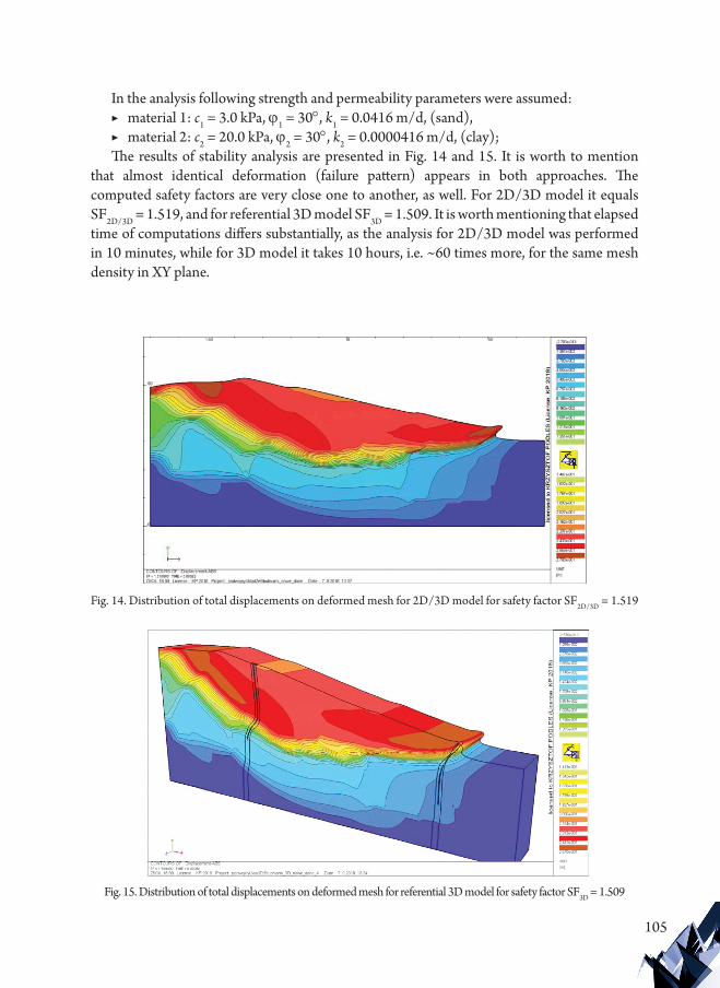
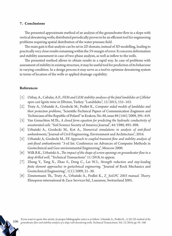