Meshless Point collocation Method For 1D and 2D

Groundwater Flow Simulation

By Under Supervision of

Ashvini Kumar Prof Anirban Dhar

10CE31005

Introduction

Groundwater contamination and soil pollution have been recognized as

critical environment problems therefore flow of groundwater must be

analysed.

Analysing flow of ground water through analytical method or numerical

methods like FEM and FDM or boundary element method is complex.

Meshfree method is a powerful numerical technique to obtain more accurate

approximate solutions in a more convenient manner for complex systems.

This method is used to establish algebraic equation for the whole problem

domain without the use of pre-defined mesh.

Different from FDM and FEM, Mfree method use a set of scatted nodes in the

problem domain and boundaries of the domain.

In present project, Mfree model is developed for groundwater flow problems

in 1D and 2D based on collocation techniques.

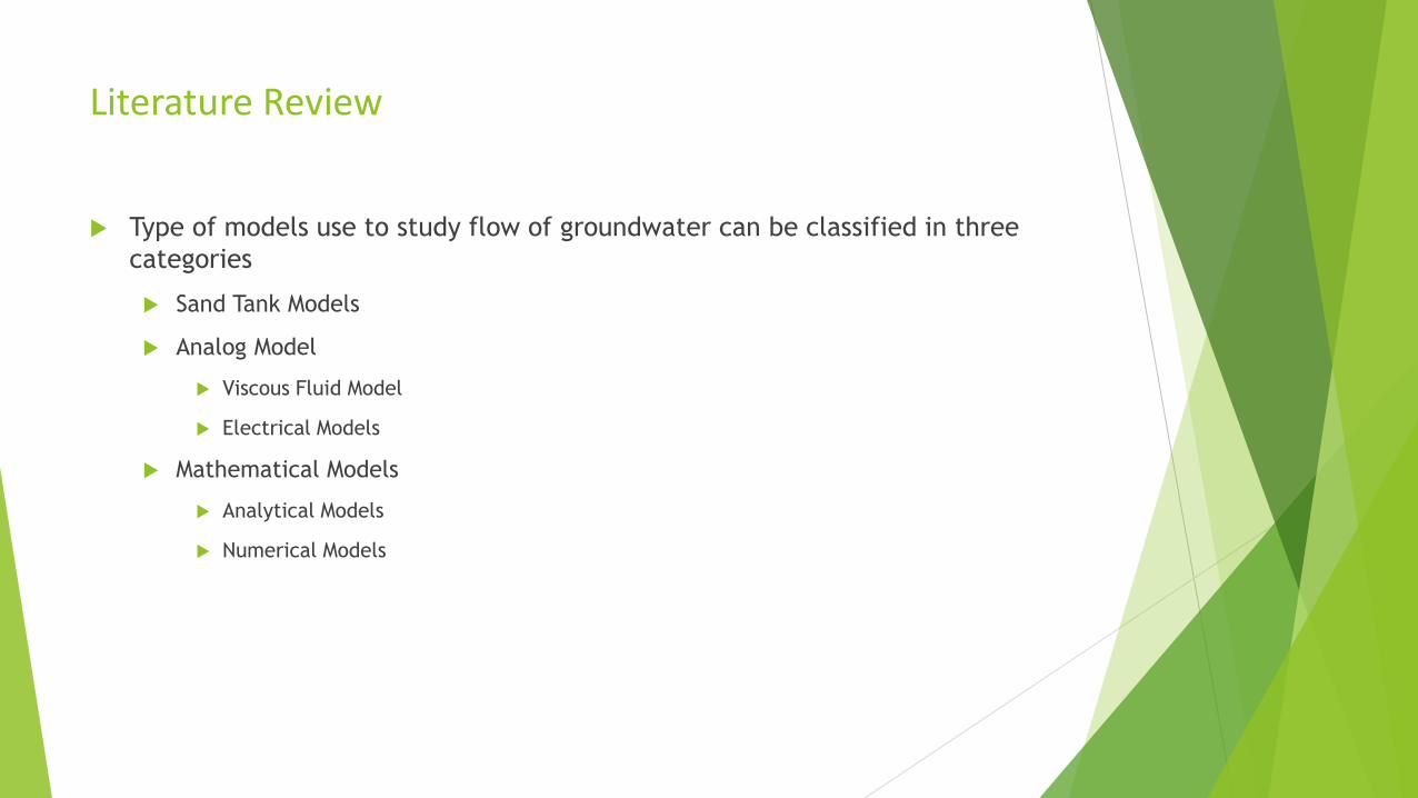
Literature Review

Type of models use to study flow of groundwater can be classified in three

categories

Sand Tank Models

Analog Model

Viscous Fluid Model

Electrical Models

Mathematical Models

Analytical Models

Numerical Models

Problem Description

In this project, a meshless method called as Polynomial Point collocation method

(PPCM) with radial basis function has been developed for the groundwater flow

simulation in porous media in one and two dimensions. The developed model has

been applied for computing head distribution in a hypothetical confined aquifer

having different boundary conditions and source, and sink terms. The developed

model is tested with analytical and FEM solutions available in literature and

found to be satisfactory.

Development of PPCM Equation for analysis of flow of groundwater

Governing equation of flow of groundwater

PPCM formulation for 1D transient Flow equation for confined aquifer

The transient of groundwater in homogeneous isotropic media in 1D can be

written as

Where, K is hydraulic conductivity (m/d) of the aquifer

Sy is specific yield

To use Mfree method, the first step is to define the trial solution as

where, is unknown head

is the shape function at node I

n is the total number of nodes in the support domain

is given by

and

ℎ𝑖

PPCM formulation for 1D transient Flow equation for confined aquifer For MQ-RBF, q=0.5, therefore can be written as

and therefore

and

Using earlier introduce equation, we get

Arranging previous equation, we get

(PPCM model for 1D flow of groundwater)

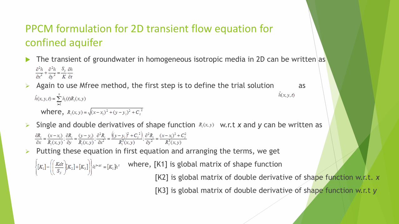
PPCM formulation for 2D transient flow equation for confined aquifer

The transient of groundwater in homogeneous isotropic media in 2D can be written as

Again to use Mfree method, the first step is to define the trial solution as

where,

Single and double derivatives of shape function w.r.t x and y can be written as

Putting these equation in first equation and arranging the terms, we get

where, [K1] is global matrix of shape function

[K2] is global matrix of double derivative of shape function w.r.t. x

[K3] is global matrix of double derivative of shape function w.r.t y

Model Development

Support Domain and Collocation Point

1D Model 2D Model

Verification of 1D Model

Verification of 1D model

Verification of 2D Model

Verification of 2D ModelNode No. t=0.2 days t=1day

Analytical FEM % Error

(analytical

with FEM)

PPCM %Error

(Analytical with

PPCM)

FEM PPCM %Difference

FEM with

PPCM

29 97.013 96.993 0.02 97.0316 0.019 97.2316 97.2316 0.084

43 93.804 93.768 0.036 93.7606 0.046 94.0059 94.0059 0.047

57 90.095 90.051 0.044 90.0756 0.022 90.0245 90.0245 0.133

71 85.451 85.413 0.038 8 0.07 85.6105 85.6105 0.041

85 78.983 78.974 0.009 78.9544 0.024 78.8544 78.8544 0.272

99 67.953 67.762 0.191 67.8552 0.144 67.8212 67.8212 0.204

Verification of 2D Model

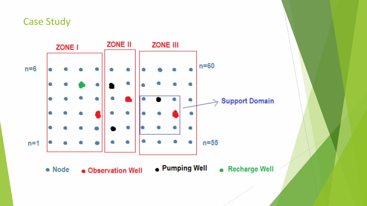
Case Study

Case Study

Properties ZONE I ZONE II ZONE III

Transmissivity Tx (m2/d) 500 400 250

Transmissivity Ty (m2/d) 300 250 200

Porosity 0.2 0.25 0.15

Case Study

Node No. FEM PPCM % Difference

21 98.2 98.149 0.0129

34 97.1 96.927 0.0445

51 95.25 95.313 0.0165

Case Study

Thank You All