7 Parallel Programming and Parallel Algorithms 7.1 INTRODUCTION Algorithms in which operations must be executed step by step are called serial or sequential algorithms. Algorithms in which several operations may be executed simultaneously are referred to as parallel algorithms. A parallel algorithm for a parallel computer can be defined as set of processes that may be executed simultaneously and may communicate with each other in order to solve a given problem. The term process may be defined as a part of a program that can be run on a processor. In designing a parallel algorithm, it is important to determine the efficiency of its use of available resources. Once a parallel algorithm has been developed, a measurement should be used for evaluating its performance (or efficiency) on a parallel machine. A common measurement often used is run time. Run time (also referred to as elapsed time or completion time) refers to the time the algorithm takes on a parallel machine in order to solve a problem. More specifically, it is the elapsed time between the start of the first processor (or the first set of processors) and the termination of the last processor (or the last set of processors). Various approaches may be used to design a parallel algorithm for a given problem. One approach is to attempt to convert a sequential algorithm to a parallel algorithm. If a sequential algorithm already exists for the problem, then inherent parallelism in that algorithm may be recognized and implemented in parallel. Inherent parallelism is parallelism that occurs naturally within an algorithm, not as a result of any special effort on the part of the algorithm or machine designer. It should be noted that exploiting inherent parallelism in a sequential algorithm might not always lead to an efficient parallel algorithm. It turns out that for certain types of problems a better approach is to adopt a parallel algorithm that solves a problem similar to, but different from, the given problem. Another approach is to design a totally new parallel algorithm that is more efficient than the existing one [QUI 87, QUI 94]. In either case, in the development of a parallel algorithm, a few important considerations cannot be ignored. The cost of communication between processes has to be considered, for instance. Communication aspects are important since, for a given algorithm, communication time may be greater than the actual computation time. Another consideration is that the algorithm should take into account the architecture of the computer on which it is to be executed. This is particularly important, since the same algorithm may be very efficient on one architecture and very inefficient on another architecture. This chapter emphasizes two models that have been used widely for parallel programming: the shared-memory model and the message-passing model. The shared-memory model refers to programming in a multiprocessor environment in which the communication between processes is achieved through shared (or global) memory, whereas the message-passing model refers to programming in a multicomputer environment in which the communication between processes is achieved through some kind of message-switching mechanism. In a multiprocessor environment, communication through shared memory is not problem free; erroneous results may occur if two processes update the same data in an unacceptable order. Multiprocessors usually support various synchronization instructions that can be used to prevent these types of errors; some of these instructions are explained in the next section. In contrast to multiprocessors, in a multicomputer environment updating data is not a problem. Memory is unshared and localized to each processor. However, message-passing is the main concern here, and usually

certain communication instructions are implemented for sending and receiving messages. This chapter discusses the issues involved in parallel programming and the development of parallel algorithms. Various approaches to developing a parallel algorithm are explained. Algorithm structures such as the synchronous structure, asynchronous structure, and pipeline structure are described. A few terms related to performance measurement of parallel algorithms are presented. Finally, examples of parallel algorithms illustrating different design structures are given. 7.2 PROGRAMMING MODELS In this section, two types of parallel programming are discussed: 1) parallel programming on multiprocessors, and 2) Parallel Programming on Multicomputers. 7.2.1 Parallel Programming on Multiprocessors To write parallel programs in a particular language in a multiprocessor environment, we need to be able to perform certain operations through the language, such as synchronization. Some of these operations are discussed in depth in the following sections. Process creation. A parallel program for a multiprocessor can be defined as a set of processes that may be executed in parallel and may communicate with each other to solve a given problem. For example, in a UNIX operating system environment, the creation of a process is done with a system call called fork. When a process executes the fork system call, a new slave (or child) process will be created, which is a copy of the original master (or parent) process. The slave process begins to execute at the point after the fork call. The fork function returns the UNIX process id of the created slave process to the master process and returns 0 to the slave process. The following code makes this concept more clear. return_code = fork (); if ( return_code = = 0 ) { slave (); -- the slave process goes to work here -- by calling slave routine

exit (0); -- slave process returns from work and terminates } else { if ( return_code = = -1 ) print ( "failure in creating a slave process " ); else -- master process continues the execution from -- this point } In this code, the fork function returns 0 in the slave process's copy of the return_code, and returns the UNIX process id of the slave process to the master process’s copy of the return_code. Note that both processes have their own copy of the return_code in separate memory locations. Synchronization. In a multiprocessor environment, processes usually communicate through shared data. This eliminates the need to make multiple copies of the same data. Having only one copy of data shared by many processes saves memory and also avoids the updating problem usually experienced when multiple copies of the same data item exist. However, shared data are not problem free and, in fact, the programmer must be careful in executing and accessing them. If two processes access the same data at the same time and use that data in a computation and then update the data using the computed result, invalid results may occur. Therefore, access to such shared data must be mutually exclusive. To understand the need for mutual exclusion, let us consider the execution of the following statement for

incrementing a shared variable index: index = index + 1;

This statement causes a read operation followed by a write operation. The read operation gets the old value of the variable index, and the write operation stores the new value. The actual computation of index+1 occurs between the read and write operations. Now assume that there are two processes, P1 and P2, each trying to increment the variable index using a statement like the preceding one. If the initial value of index is 5, the correct final value index should be 7 after both processes have incremented it. In other words, index is incremented twice, once for each process. However, an invalid result can be obtained if one process accesses variable index while it is being incremented by the other process (between the read and write operations). For example, it is possible that process P1 reads the value 5 from index, and then process P2 reads the same value 5 from index before P1 gets a chance to write the new value back to memory. In this case, the final value of index will be 6, obviously an invalid result. Therefore, access to the variable index must be mutually exclusive—accessible to only one process at a time. To ensure such mutual exclusion, a mechanism, called synchronization must be implemented that allows one process to finish writing the final value of the variable index before the other process can have access to the same variable. Multiprocessors usually support various simple instructions (sometimes referred to as mutual exclusion primitives) for synchronization of resources and/or processes. Often, these instructions are implemented by a combination of hardware and software. They are the basic mechanisms that enforce mutual exclusion for more complex operations implemented in software macros. (A macro is a single instruction that represents a given sequence of instructions in a program.) A common set of basic synchronization instructions is defined next. Lock and Unlock. Solutions to mutual exclusion problems can be constructed using mechanisms referred to as locks. A process that attempts to access shared data that is protected with a locked gate waits until the associated gate is unlocked and then locks the gate to prevent other processes having access the data. After the process accesses and performs the required operations on the data, the process unlocks the gate to allow another process to access the data. The important characteristic of lock and unlock operations is that they are executed atomically, that is, as uninterruptible operations; in other words, once they are initiated, they do not stop until they complete. The atomic operations of lock and unlock can be described by the following segments of code:

Lock(L) { while (L= =1) NOP; -- NOP stands for no operation L = 1; } Unlock(L) { L = 0; }

In this code, the variable L represents the status of the protection gate. If L=1, the gate is interpreted as being closed. Otherwise, when L=0, the gate is interpreted as being open. When a process wants to access shared data, it executes a Lock(L) operation. This atomic operation repeatedly checks the variable L until its value becomes zero. When L is zero, the Lock(L) operation sets its value to 1. An Unlock(L) operation causes L to be reset to 0. To understand the use of lock and unlock operations, consider the previous example in which two processes were incrementing the shared variable index by executing the following statement:

index = index + 1; To ensure a correct result, a lock and an unlock operation can be inserted in the code of each process as follows:

Lock(L) index = index + 1; Unlock(L)

Now, each process must execute a Lock(L) instruction before changing the variable index. After a process completes execution of the Lock(L) instruction, the other process [if it tries to execute its own Lock(L) instruction] will be forced to wait until the first process unlocks the variable L. When the first process finishes executing the index = index + 1 statement, it executes the Unlock(L) instruction. At this time, if the other process is waiting at the Lock(L) instruction, it will be allowed to proceed with execution. In other words, the Lock(L) and Unlock(L) statements create a kind of "fence" around the statement index=index+1, such that only one process at a time can be inside the fence to increment index. The statement index=index+1 is often referred to as a critical section. In general, a critical section is a group of statements that must be executed or accessed by at most a certain number of processes at any given time. In our previous example, it was assumed at most one process could execute the critical section index=index+1 at any given time. In general, a structure that provides exclusive access to a critical section is called a monitor. Monitors were first described by Hoare [HOA 74] and have become a main mechanism in parallel programming. A monitor represents a serial part of a program. As is shown in Figure 7.1, a monitor represents a kind of fence around the shared data. Only one process can be inside the fence at a time. Once inside the fence, a process can access the shared data.

Figure 7.1 Structure of a monitor; it provides exclusive access to a shared data.

The following statements represent the general structure of a monitor.

Lock(L) <Critical Section>

Unlock(L) A lock instruction is placed before a critical section, and the unlock instruction is placed at the end of the critical section. When a process wishes to invoke the monitor, it attempts to lock the lock variable L. If the monitor has already been invoked by another process, the process waits until the process that initiated the lock instruction releases the monitor by unlocking the lock variable. Only one process can invoke the monitor; other processes queue up waiting for the process to release the monitor. This limits the amount of parallelism that can be obtained in a program. Therefore, minimizing the amount of code in a critical section will increase parallel performance for most parallel algorithms. In the preceding implementations of lock, the variable L is repeatedly checked until its value becomes zero. This type of lock, which causes the processor to be tied up in an idle loop while increasing the memory contention, is called spin lock. To prevent repeatedly checking the variable L while it is 1, an interrupt mechanism can be used. In this case, a lock is called a suspended lock. Whenever a process fails to obtain the lock, it goes into a waiting state. When a process releases the lock, it signals all (or some) of the waiting processes through some kind of interrupt mechanism. One way of implementing such a mechanism could be the use of interprocessor interrupts. Another option could be a software implementation of a queue for enqueueing the processes in the waiting state. The lock instruction is often implemented in multiprocessors by using a special instruction called Test&Set. The Test&Set instruction is an atomic operation that returns the current value of a memory cell and sets the

memory cell to 1. Both phases of this instruction (i.e., test and set) are implemented as one uninterruptible operation in the hardware. Once a processor executes such an instruction, no other processor can intervene in its execution. In general the operation of a Test&Set instruction can be defined as follows:

Test&Set(L) . { temp = L; L = 1; return temp; . } Reset(L) { L = 0; }

This Test&Set instruction copies the contents of the variable L to the variable temp and then sets the value of L to 1. If a multiprocessor supports the Test&Set instruction, then the Lock and Unlock instructions can be implemented in software as follows:

Lock(L) { while (Test&Set(L)= =1) NOP; } Unlock(L) { Reset(L) }

In practice, most multiprocessors are based on commercially available microprocessors. Often, these microprocessors support basic instructions that are similar to the Test&Set instruction. For example, the Motorola 88000 processor series supports an instruction, called exchange register with memory (Xmem), for implementing synchronization instructions in multiprocessor systems. Similarly, the Intel Pentium processor provides an instruction, called exchange (Xchg) for synchronization. The Xmem and Xchg instructions exchange the contents of a register with a memory location. For example, let L be the address of a memory location and R be the address of a register. Then Xchg can be defined as follows:

Xchg(L,R) { temp = L; L = R; R = temp; }

In general the exchange instructions require a sequence of read, modify, and write cycles. During these cycles the processor should be allowed atomic access to the location that is referenced by the instruction. To provide such atomic access, often the processors accommodate a signal that indicates to the outside world that the processor is performing a read-modify-write sequence of cycles. For example, the Pentium processor provides an external signal, called lock#, to perform atomic accesses of memory [INT 93a, INT 93b]. When lock# is active, it indicates to the system that the current sequence of bus cycles should not be interrupted. That is, a programmer can perform read and write operations on the contents of a memory variable and be assured that the variable is not accessed by any other processor during these operations. This facility is provided for certain instructions when followed by a Lock instruction and also for instructions that implicitly perform read-modify-write cycles such as the Xchg instruction. When a Lock instruction is executed, it activates the lock# signal during the execution of the instruction that follows.

To implement a spin lock, a processor can acquire a lock with an Xchg (or Xmem) instruction. The Xchg performs an indivisible read-modify-write bus transaction that ensures exclusive ownership of the lock. Therefore, an alternative implementation for Lock and Unlock instructions could be as follows:

Lock(L) { R =1; while (R= =1) Xchg(L,R); } Unlock(L) { L=0; }

Wait and Signal (or Increment and Decrement). An alternative to Lock and Unlock instructions could be the implementation of wait and signal instructions (also referred to as increment and decrement instructions). These instructions decrement or increment a specified memory cell (location), and during their execution no other instruction can access that cell. In some situations, when more than one process is allowed to access a critical section, the protection can be obtained with fewer Wait/Signal instructions than Lock/Unlock instructions. This is because the Lock/Unlock instructions operate on a binary value (0 or 1), while the full contents of a variable Wait/Signal operate on semaphore (S). The atomic operations of wait and signal can be described by the following segment of code:

Wait(S) { while (S <= 0) NOP; S =S - 1; } Signal(S) { S =S + 1; }

For example, assume that there is a shared buffer of length k, where k processes can operate on separate cells simultaneously. When there are k processes working on the buffer, the k+1th process is forced to wait until one of the (1 to k) processes finishes its operation. A simple way to implement this form of synchronization is to start with an initial value of k in the semaphore variable S. As each process obtains a cell in the buffer, S is decremented by 1. Eventually, when k processes have obtained a cell in the buffer, S will equal 0. When a process wishes to access the shared buffer, it executes the instruction Wait (S). This instruction spins while S 0. If S>0, Wait(S) decrements S and lets the process access the shared buffer. The process executes the instruction Signal (S) after completing its operation on the shared buffer. Signal (S) increments S, which lets another process have access to the shared buffer. In summary, as shown in the following statements, in situations where more than one process is allowed to access a critical section, a Wait instruction is placed before the critical section and a Signal instruction is placed at the end of that section.

Wait(semaphore) <Critical Section> Signal(semaphore)

Fetch&Add. One problem with the preceding synchronization methods is when a large number of Lock

(or Wait) instructions is issued for execution simultaneously. When n processes attempt to access a shared data simultaneously, n Lock (or Wait) instructions will be executed, one after the other, even though only one process will successfully access data. Although the memory contention produced by the simultaneous access may not degrade the performance so much for a small number of processes, it may become a bottleneck as the number of processes increases. For systems with a large number of processors, for example 100 to 1000, a mechanism for parallel synchronization is necessary. One such mechanism, which is used in some parallel machines, is called Fetch&Add. The instruction Fetch&Add(x,c) increases a shared-memory location x with a constant value c and returns the value of x before the increment. The semantics of this instruction are

Fetch&Add(x,c) { temp = x; x = temp + c; return temp; }

If n processes issue the instruction Fetch&Add(x,c) at the same time, the shared-memory location x is updated only once by adding the value n*c to it, and a unique value is returned to each of the n processes. Although the memory is updated only once, the values returned to each process are the same as when an arbitrary sequence of n Fetch&Adds is sequentially executed. To show the effectiveness of the Fetch&Add instruction, let us consider the problem of adding two vectors in parallel.

for (i=1; i<=k; i++) { Z[i] = A[i] + B[i] ; }

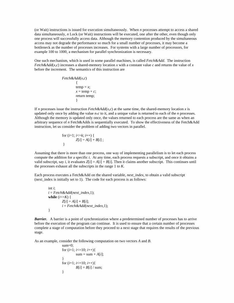
Assuming that there is more than one process, one way of implementing parallelism is to let each process compute the addition for a specific i. At any time, each process requests a subscript, and once it obtains a valid subscript, say i, it evaluates Z[i] = A[i] + B[i]. Then it claims another subscript. This continues until the processes exhaust all the subscripts in the range 1 to K. Each process executes a Fetch&Add on the shared variable, next_index, to obtain a valid subscript (next_index is initially set to 1). The code for each process is as follows: int i; i = Fetch&Add(next_index,1); while (i<=K) { Z[i] = A[i] + B[i]; i = Fetch&Add(next_index,1); } Barrier. A barrier is a point of synchronization where a predetermined number of processes has to arrive before the execution of the program can continue. It is used to ensure that a certain number of processes complete a stage of computation before they proceed to a next stage that requires the results of the previous stage. As an example, consider the following computation on two vectors A and B.

sum=0; for (i=1; i<=10; i++){ sum = sum + A[i]; } for (i=1; i<=10; i++){ B[i] = B[i] / sum; }

Assume that there are two processes, with id 0 and 1, performing the computation in two stages: stage 1 and stage 2. Also, assume that the variable sum and vectors A and B are defined as shared variables and are accessible to both processes. The shared variable sum has been initialized to 0. In stage 1 of the computation, both processes contribute to the calculation of the variable sum. To the variable sum, process 0 adds the values A[1], A[3], A[5], A[7], and A[9], and process 1 adds the values A[2], A[4], A[6], A[8], and A[10]. When both processes complete their contribution to the sum, they proceed to the second stage of computation. In stage 2, process 0 computes the new values for B[1], B[3], B[5], B[7], and B[9], and process 1 computes the new values for B[2], B[4], B[6], B[8], and B[10]. The following code gives the main steps of each process.

int i, partial_sum; partial_sum=0; for (i=1+id; i<=10; i=i+2){ -- id refers to process id; -- it is either 0 or 1.

partial_sum = partial_sum + A[i]; } Lock(L) sum = sum + partial_sum; Unlock(L) BARRIER(2) -- none of the processes can continue past -- the barrier statement until both

-- processes have arrived at this statement for (i=1+id; i<=10; i=i+2){ B[i] = B[i] / sum; }

In this code, each process uses a local variable partial_sum to add five elements of vector A. Once the partial_sum is calculated, it is added to the shared variable sum. To ensure a correct result, a Lock instruction is executed before changing the sum. The BARRIER macro prevents processes updating elements of vector B until both processes have completed stage 1 of computation. In general, a barrier can be implemented in software using spin locks. Assume that n processes must enter the barrier before program execution can continue. When a process enters the barrier, the barrier checks to see how many processes have already been blocked. (Processes that are waiting at the barrier are called blocked processes.) If the number of blocked processes is less than n-1, the newly entered process is also blocked. On the other hand, if the number of blocked processes is n-1, then all the blocked processes and the newly entered process are allowed to continue execution. The processes continue by executing the statement following the barrier statement. The following code gives the main steps of a barrier macro for synchronizing n processes:

BARRIER(n) { Lock(barrier_lock) if(number_of_blocked_processes < n - 1 ) BLOCK WAKE_UP }

Let number_of_blocked_processes denote a shared variable that holds the total number of processes that have entered the barrier so far. Initially, the value of this variable is set to 0. A process entering the barrier will execute the BLOCK macro when there are not n-1 processes in the blocked stage yet. The BLOCK macro causes the process executing it to be suspended by adding it to the set of blocked processes and also releases the barrier by executing Unlock(barrier_lock). Whenever there are n-1 blocked processes, the nth process entering the barrier executes the WAKE_UP macro and then leaves the barrier without unlocking

the barrier_lock. The WAKE_UP macro causes a process (if there is one) to be released from the set of blocked processes. The released process will continue its execution at the point where it was suspended, that is, it executes the WAKE_UP macro and then exits the barrier. This process continues until all of the suspended processes leave the barrier. The last process, right before leaving the barrier, releases the barrier by executing Unlock(barrier_lock). The following code gives a possible implementation for the barrier macro. In this code, the macros BLOCK and WAKE_UP are implemented in a simple form using spin lock.

BARRIER(n) { Lock(barrier_lock) if(number_of_blocked_processes < n - 1 ) -- code for BLOCK macro { number_of_blocked_processes = number_of_blocked_processes +1; Unlock(barrier_lock) Lock(block_lock) }

if(number_of_blocked_processes > 0) -- code for WAKE_UP macro { number_of_blocked_processes = number_of_blocked_processes -1; Unlock(block_lock) } else Unlock(barrier_lock) }

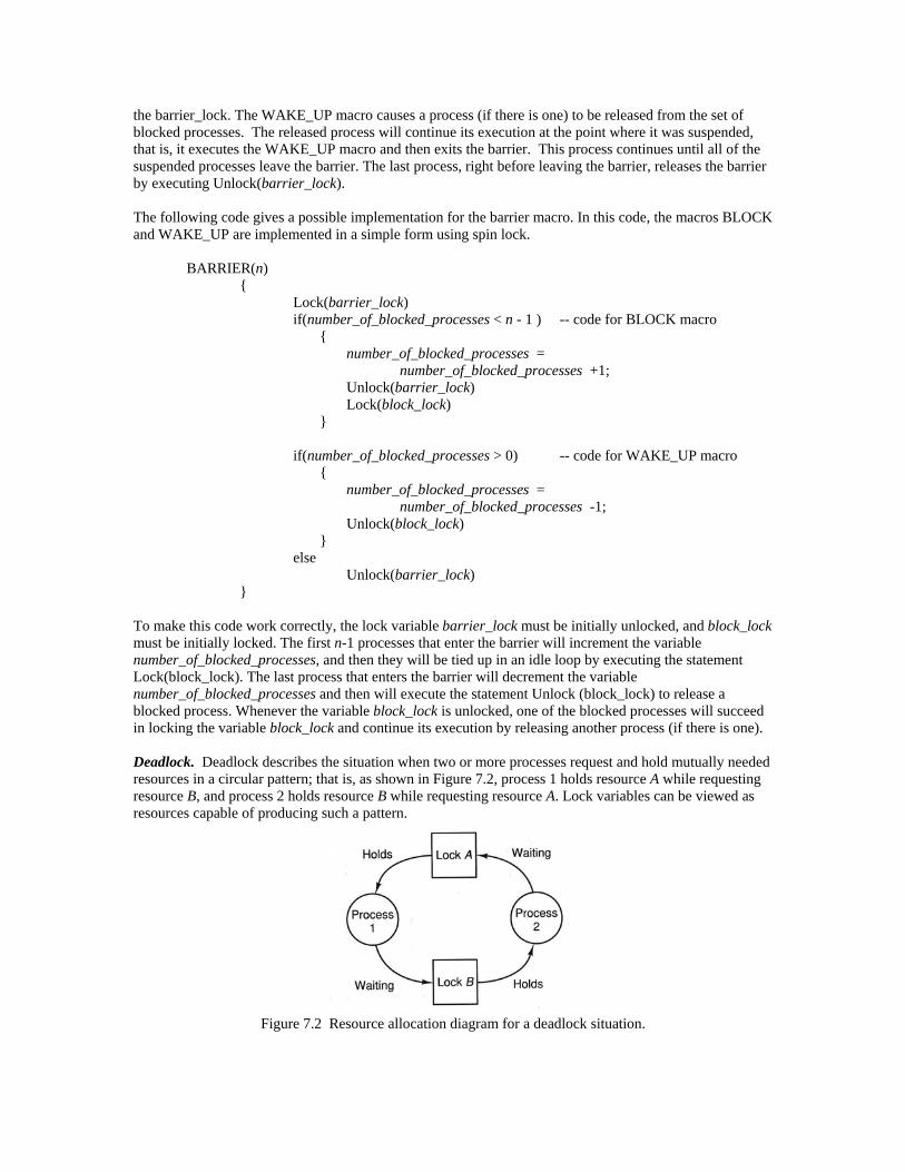
To make this code work correctly, the lock variable barrier_lock must be initially unlocked, and block_lock must be initially locked. The first n-1 processes that enter the barrier will increment the variable number_of_blocked_processes, and then they will be tied up in an idle loop by executing the statement Lock(block_lock). The last process that enters the barrier will decrement the variable number_of_blocked_processes and then will execute the statement Unlock (block_lock) to release a blocked process. Whenever the variable block_lock is unlocked, one of the blocked processes will succeed in locking the variable block_lock and continue its execution by releasing another process (if there is one). Deadlock. Deadlock describes the situation when two or more processes request and hold mutually needed resources in a circular pattern; that is, as shown in Figure 7.2, process 1 holds resource A while requesting resource B, and process 2 holds resource B while requesting resource A. Lock variables can be viewed as resources capable of producing such a pattern.

Figure 7.2 Resource allocation diagram for a deadlock situation.

There can be more than one lock variable declared and used in a program. Since lock instructions can be placed almost anywhere in the program and numerous lock variables can exist, it is the responsibility of the programmer to use them with care. Deadlock may occur if a process attempts to lock another critical section while it is working in its own critical section. One possible deadlock scenario is as follows: ___________________________________________________ At time Process 1 Process 2 ___________________________________________________ t0 Lock(A) t1 Lock(B) t2 Lock(B) t3 Lock(A) . . ___________________________________________________ It is assumed that time t0<t1<t2<t3. At time t0, process 1 locks the lock variable A. Later, at time t1, process 2 locks the lock variable B. At time t2 and t3, processes 1and 2 attempt to lock the lock variables B and A, respectively. However, they cannot succeed, since neither has released the previous lock. Therefore, processes 1 and 2 are both busy waiting at the second lock, each denying the other access to the resources they need. Thus a deadlock situation has occurred. 7.2.2 Parallel Programming on Multicomputers A multicomputer, also referred to as a message-passing concurrent computer, consists of several processors called nodes, which are connected with an interconnection network. Each processor has its own local memory. Thus, in contrast to the shared-memory multiprocessor, there is no global memory. That is, in a multicomputer the nodes are not able to coordinate themselves through global variables, but coordinate their activities by sending messages to each other. The messages are sent and received through communication channels that are implemented in each node. Similar to the programming in the multiprocessor environment, whenever the master process creates a slave process, a new process id will be produced and will be known to both of the processes. The processes use these ids as addresses for sending messages to each other. In addition to the process id, the master process also specifies the name of the node that executes the created slave. Once some processes are created, message-passing between them can be initiated. A message may be either a control message or a data message and may contain from 1 byte of information to any size that will fit in the node's memory. The messages may be routed through different routing paths according to their length and/or destination address. However, these differences are invisible to the programmer. Usually, messages may be queued as necessary in the sending node, in transit, and in the receiving node. That is, a message may have an arbitrary delay from sender to receiver. However, their ordering is usually preserved through the network. Each message carries some additional information, such as the destination process id and message length. In some implementations, it also carries the source process id. Whenever a process wants to send a message, it first allocates a buffer for the message. Once the message has been built in the allocated buffer, the process issues a send command. These are represented as

p = mem_allocate (message_length); -- p points to the allocated buffer send (p, message_length, source_id, destination_id);

A process can receive a message by issuing:

p = receive_b( ); The character b at the end of receive_b indicates that this command is a blocking function, which means it

does not return until a message has arrived for the process. The receive_b function allocates a buffer equal to the size of the received message and returns p, a pointer to the buffer that contains the received message. (This buffer might also be allocated by the user.) If a nonblocking receive command, denoted as receive( ), is used, it may return a null pointer if there is no message queued for the process. In contrast to multiprocessors, in a multicomputer system, processor-to-memory communication is not a problem because memory is localized to each processor in a node. Interprocess message-passing happens less frequently than memory access. Although interprocess communication exhibits a larger delay, it does not present an obstacle to building a system with thousands of nodes [ATH 88]. Although the message-passing model is well suited for multicomputers, we can also implement a message-passing communication environment on a multiprocessor. One way to do this is to implement a communication channel by defining a channel buffer and a pair of pointers to this channel buffer. One pointer indicates the next location in the buffer to be written to by the transmitting process, while the other pointer indicates the next location to be read by the receiving process. Another way of communication can be as simple as one process writing to a specific memory location, called a mailbox, and another process reading the mailbox. To prevent a message from being overwritten by the transmitting process before it is read by another process, and/or the receiving process reads an invalid message, communication is often implemented by mutually exclusive access to a mailbox. 7.3 PARALLEL COMPUTATION To make a program suitable for execution on a parallel computer, it must be decomposed into a set of processes, which will then make up the parallel algorithm. Decomposition involves partitioning and assignment. Partitioning has been defined as specifying the set of tasks (or work) that will implement a given problem on a specified parallel computer in the most efficient manner [LIN 81]. Assignment is the process of allocating the partitions or tasks to processors. Partitioning and assignment are discussed in the following. 7.3.1 Partitioning The performance of a parallel algorithm depends on program granularity. Granularity refers to the size of the task for a process compared to implementation overhead (such as synchronization, critical section resolution, and communication). As the size of each individual task increases, the amount of computation per task becomes much higher than the amount of implementation overhead per task. Therefore, one solution to parallel computation is to partition the problem into several large size tasks. This is referred to as coarse-granularity parallelism. However, a large-sized task decreases the number of required processes and therefore reduces the amount of parallelism. An alternative would be to partition a problem into a number of relatively small size tasks that can run in parallel. This is referred to as fine-granularity parallelism. In general, a fine-granularity task contains a small number of instructions, which may cause the amount of computation per task to become much smaller than the amount of implementation overhead. Thus, to improve the performance of a parallel algorithm, the designer should consider the trade-offs between computation and implementation overhead. This is a similar concept to the one for designing a sequential algorithm, for which a designer should consider the trade-offs between memory space and execution time. A general solution for balancing between computation and overhead is clustering. The idea of clustering is to form groups of task such that the amount of overhead within groups is much greater than the amount of overhead between groups. In practice, the number of processors is usually adjusted to the size of the problem in order to keep the run time in a certain desired range. To achieve this goal, it is important that the algorithm utilizes all the processors by giving them a task and keeping the ratio of overhead time to computational time low for each task. If this can be accomplished for any number of processors (1 to n), then the algorithm is called scalable. It may not be possible to develop a scalable algorithm for some architectures unless the problem holds certain features. For example, to have a scalable algorithm for a problem on a hypercube

multicomputer, the nature of the problem should allow localizing communication between neighbor nodes. This is because a hypercube's longest communication path increases as log2N, where N is the number of nodes. Some scientific problems that require the solution of partial differential equations can be mapped to a hypercube such that each node needs to communicate only with its immediate neighbors [GUS 88a, DEN 88]. There are two methods of partitioning tasks: static partition and dynamic partition. The static partition method partitions the tasks before execution. The advantage in this method is that there is less communication and contention among processes. The disadvantage is that input data may dictate how much parallel computation actually occurs at run time and how much of the data is to be given to a process; as a result, some processes may not be kept busy during execution. The dynamic partition method partitions the tasks during execution. The advantage to dynamic partitioning is that it tends to keep processes busier, and it is not as affected by the input data as is the static partition method. The disadvantage is the amount of communication by processes that is needed in implementing such a scheme. Processes may be created such that all processes perform the same function on different portions of the data or such that each performs a different function on the data. The former approach is referred to as data partitioning (also referred to as data parallelism), while the latter is often referred to as function partitioning (also referred to as control parallelism or sometimes functional parallelism). Since data partitioning involves the creation of identical processes, it is also referred to as homogeneous multitasking. For a similar reason, function partitioning is sometimes referred to as heterogeneous multitasking by which multiple unique processes perform different tasks on data. (The multiplicity of terms is understandably confusing, however, due to the recentness of study in this area, it is also to be expected.) The data partitioning approach extracts parallelism from the organization of problem data. The data structure is divided into pieces of data, with each piece being processed in parallel. A piece of data can be an individual item of data or a group of individual items. Data partitioning is especially useful in solving numerical problems that deal with large arrays and vectors. It is also a useful method to nonnumerical problems such as sorting and combinatorial search. This approach, in particular, is suited for the development of algorithms in multicomputers, because a processor mainly performs computation on its own local data and seldom communicates with other processors. The following example illustrates data partitioning and function partitioning. Consider the following computation on four vectors A, B, C, and D.

Z[i] = (A[i] * B[i]) + (C[i] / D[i]), for i=1 to 10. When data partitioning is applied, this computation is performed as follows: 10 identical processes are created such that each process performs the computation for a unique index i. Here, parallelism has been achieved by computing each Z[i] simultaneously using multiple identical processes. When function partitioning is applied, two different processes, P1 and P2, are created. P1 performs the computation x = A[i] * B[i] and sends the value of x to P2. P2 in turn computes y = C[i] / D[i], and after it receives the value of x from P1 it performs the computation Z[i] = x + y. This is done for each index i. Here, parallelism has been achieved by performing the functions of multiplication and division simultaneously. Generally, in the function partitioning approach the program is organized such that the processes take advantage of parallelism in the code, rather than in the data. On the whole, data partitioning offers the following advantages over function partitioning:

1. Higher parallelism. 2. Equally balanced load among processes (this is because all processes are identical with respect to

the computation being performed). 3. Easier to implement.

7.3.2 Assignment or Scheduling In the previous section, the problem of partitioning was discussed. Once a program is partitioned into processes, each process has to be assigned to a processor for execution. This mapping of processes to processors is referred to as assignment or scheduling. Assignment may be static or dynamic. In static assignment, the set of processes and the order in which they must be executed are known prior to execution. Static assignment algorithms require low process communication and are well suited when process communication is expensive. Also, in this type of assignment, scheduling costs are incurred only once whenever the same program runs many times on different data. In contrast to static assignment, in dynamic assignment processes are assigned to processors at run time. Dynamic assignment is well suited when process communication is inexpensive. It also offers better utilization of processors and provides flexibility in the number of available processors. This is particularly useful when the number of processes depends on the input size. The drawbacks associated with dynamic assignment are the following:

1. The structure of the program becomes hard to understand. 2. Deadlock detection becomes difficult. 3. Since processes are assigned at run time, the performance analysis of the program sometimes

becomes impossible. 4. There is more communication and contention among processes.

7.4 ALGORITHM STRUCTURES A parallel algorithm for parallel computers can be defined as a collection of concurrent processes operating simultaneously to solve a given problem. These algorithms can be divided into three categories: synchronous, asynchronous, and pipeline structures. 7.4.1 Synchronous Structure In this category of algorithms, two or more processes are linked by a common execution point used for synchronization purposes. A process will come to a point in its execution where it must wait for other (one or more) processes to reach a certain point. After processes have reached the synchronization point, they can continue their execution. This leads to the fact that all processes that have to synchronize at a given point in their execution must wait for the slowest one. This waiting period is the main drawback for this type of algorithm. Synchronous algorithms are also referred to as partitioning algorithms. Large-scale numerical problems (such as those solving large systems of equations) expose an opportunity for developing synchronous algorithms. Often, techniques used for these problems involve a series of iterations on large arrays. Each iteration uses the partial result produced from the previous iteration and makes a step of progress toward the final solution. The computation of each iteration can be parallelized by letting many processes work on different parts of the data array. However, after each iteration, processes should be synchronized because the partial result produced by one process is to be used by other processes on the next iteration. Synchronous parallel algorithms can be implemented on both shared-memory models and message-passing models. When synchronous algorithms are implemented on a message-passing model, communication between processes is achieved explicitly using some kind of message-passing mechanism. When implemented on a shared-memory model, depending on the type of problem to be solved, two kinds of communication strategies may be used. Processes may communicate explicitly using message passing or implicitly by referring to certain parts of memory. These communication strategies are illustrated in the following.

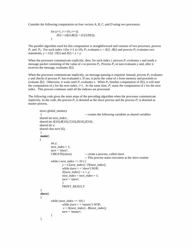
Consider the following computation on four vectors A, B, C, and D using two processors.

for (i=1; i<=10; i++){ Z[i] = (A[i]*B[i]) + (C[i]/D[i]);

} The parallel algorithm used for this computation is straightforward and consists of two processes, process P1 and P2. For each index i (for i=1 to 10), P1 evaluates x = A[i] * B[i] and process P2 evaluates two statements, y = C[i] / D[i] and Z[i] = x + y. When the processes communicate explicitly, then, for each index i, process P1 evaluates x and sends a message packet consisting of the value of x to process P2. Process P2 in turn evaluates y and, after it receives the message, evaluates Z[i]. When the processes communicate implicitly, no message-passing is required. Instead, process P2 evaluates y and checks if process P1 has evaluated x. If yes, it picks the value of x from memory and proceeds to evaluate Z[i]. Otherwise, it waits until P1 evaluates x. When P2 finishes computation of Z[i], it will start the computation of y for the next index, i+1. At the same time, P1 starts the computation of x for the next index. This process continues until all the indexes are processed. The following code gives the main steps of the preceding algorithm when the processes communicate implicitly. In the code, the process P1 is denoted as the slave process and the process P2 is denoted as master process.

struct global_memory { -- creates the following variables as shared variables shared int next_index; . shared int A[10],B[10],C[10],D[10],Z[10]; . shared int x; shared char turn [6]; } main() { int y; next_index = 1; turn = 'slave'; CREATE(slave) -- create a process, called slave. -- This process starts execution at the slave routine while ( next_index <= 10 ) { y = C[next_index] / D[next_index]; while (turn = = 'slave') NOP; Z[next_index] = x + y; next_index = next_index + 1; turn = 'slave'; } PRINT_RESULT } slave() { while (next_index <= 10) { while (turn = = 'master') NOP; x = A[next_index] * B[next_index]; turn = 'master'; } }

The vectors A, B, C, D, and Z are in global shared-memory and are accessible to both processes. Once the main process, called the master process, has allocated shared memory, it executes the CREATE macro. Execution of CREATE causes a new process to be created. The created process, called the slave process, starts execution at the slave routine, which is specified as an argument in the CREATE statement. 7.4.2 Asynchronous Structure Asynchronous parallel algorithms are characterized by letting the processes work with the most recently available data. These kinds of algorithms can be implemented on both shared-memory models and message-passing models. In the shared-memory model, there is a set of global variables accessible to all processes. Whenever a process completes a stage of its program, it reads some global variables. Based on the values of these variables and the results obtained from the last stage, the process activates its next stage and updates some of the global variables. When asynchronous algorithms are implemented on a message-passing model, a process reads some input messages after completing a stage of its program. Based on these messages and the results obtained from the last stage, the process starts its next stage and sends messages to other processes. Thus an asynchronous algorithm continues or terminates its process according to values in some global variables (or some messages) and does not wait for an input set as a synchronous algorithm does. That is, in an asynchronous algorithm, synchronizations are not needed for ensuring that certain input is available for processes at various times. Asynchronous algorithms are also referred to as relaxed algorithms due to their less restrictive synchronization constraints. As an example, consider the computation of the four vectors that was given in the previous section. Using two processes to evaluate, we have:

Z[i]=(A[i]*B[i])+(C[i]/D[i]) for i=1 to 10 (7.1) An asynchronous algorithm can be created by letting each process compute expression (7.1) for a specific i. At any time, each process requests an index. Once it obtains a valid subscript, say i, it evaluates: Z[i]=(A[i]*B[i])+(C[i]/D[i]) and then claims another subscript. That is, process P1 may evaluate Z[1] while process P2 evaluates Z[2]. This action continues until the processes exhaust all the subscripts in the range 1 to 10. The following code gives the main steps of a parallel program for the preceding algorithm.

struct global_memory { shared int next_index; shared int A[10],B[10],C[10],D[10],Z[10]; } main() { CREATE(slave) -- create a process, called slave. -- This process starts execution at the slave routine task(); WAIT_FOR_END -- wait for slave to be terminated PRINT_RESULT } slave() { task(); } task() {

int i; GET_NEXT_INDEX(i) . while (i>0) {

Z[i] = (A[i] * B[i]) + (C[i] / D[i]); GET_NEXT_INDEX(i)

} }

The vectors A, B, C, D, and Z are in global shared-memory and are accessible to both processes. Once the master process has allocated shared memory, it creates a slave process. In the slave routine, the slave process simply calls task. The master process also calls task immediately after creating the slave. In the task routine, each process executes the macro GET_NEXT_INDEX(i). The macro GET_NEXT_INDEX is a monitor operation, that is, at any time only one process is allowed to execute and modify some statements and the variables of this macro. Execution of GET_NEXT_INDEX returns in i the next available subscript (in the range 1 to 10) while valid subscripts exist; otherwise, it returns -1 in i. The macro GET_NEXT_INDEX uses the shared variable next_index to keep the next available subscript. When a process obtains a valid subscript, it evaluates Z[i] and again calls GET_NEXT_INDEX to claim another subscript. This process continues until all the subscripts in the range 1 to 10 are claimed. If the slave process receives -1 in i, it dies by returning from task to slave and then exiting from slave. If the master process receives -1 in i, it returns back to the main routine and executes the macro WAIT_FOR_END. This macro causes the master process to wait until the slave process has terminated. This ensures that all the subscripts have been processed. In comparison to synchronous algorithms, asynchronous algorithms require less access to shared variables and as a result tend to reduce memory contention problems. Memory contention occurs when different processes access the same memory module within a short time interval. When a large number of processes accesses a set of shared variables for the purpose of synchronization or communication, a severe memory contention may occur. These shared variables, sometimes called memory hot spots, may cause a large number of memory accesses to occur. The memory accesses may then create congestion on the interconnection network between processors and memory modules. The congestion will increase the access time to memory modules and, as a result, cause performance degradation. Therefore, it is important to reduce memory hot spots. This can be achieved in asynchronous algorithms by distributing data in a proper way among the memory modules. In general, asynchronous algorithms are more efficient than synchronous for the following four reasons.

1. Processes never wait on other processes for input. This often results in decreasing run time. 2. The result of the processes that are run faster may be used to abort the slower processes, which are

doing useless computations. 3. More reliable. 4. Less memory contention problems, in particular when the algorithm is based on the data

partitioning approach. However, asynchronous algorithms have the drawback that their analysis is more difficult than synchronous algorithms. At times, due to the dynamic way in which asynchronous processes execute and communicate, analysis can even be impossible. 7.4.3 Pipeline Structure In algorithms using a pipeline structure, processes are ordered and data are moved from one process to the next as though through a pipeline. Computation proceeds in steps as on an assembly line. At each step, each process receives its input from some other process, computes a result based on the input, and then passes the result to some neighboring processes. This type of processing is also referred to as macropipelining and is useful when the algorithm can be

decomposed into a finite set of processes with relationships as defined in the previous paragraph. In a pipeline structure, the communication of data between processes can be synchronous or asynchronous. In a synchronous design, a global synchronizing mechanism, such as a clock, is used. When the clock pulses, each process starts the computation of its next step. In an asynchronized design, the processes synchronize only with some of their neighbors using some local mechanism, such as message passing. Thus, in this type of design, the total computation requires less synchronization overhead than a synchronized design.

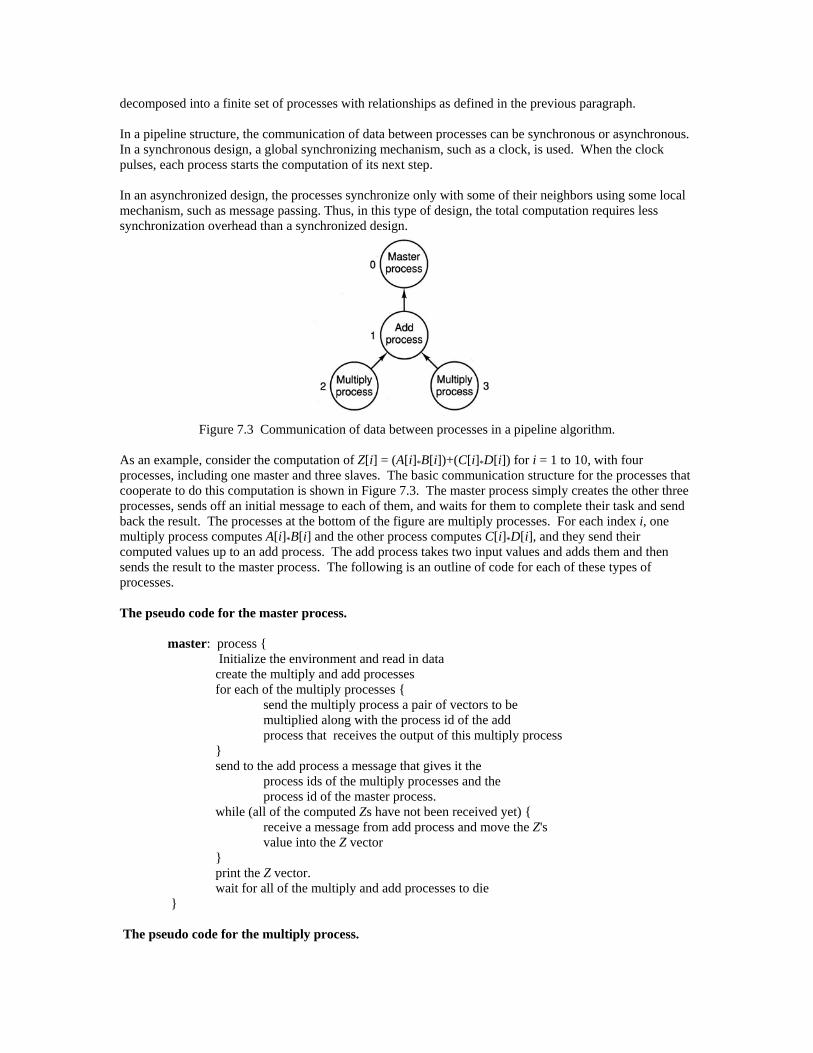
Figure 7.3 Communication of data between processes in a pipeline algorithm.

As an example, consider the computation of Z[i] = (A[i]*B[i])+(C[i]*D[i]) for i = 1 to 10, with four processes, including one master and three slaves. The basic communication structure for the processes that cooperate to do this computation is shown in Figure 7.3. The master process simply creates the other three processes, sends off an initial message to each of them, and waits for them to complete their task and send back the result. The processes at the bottom of the figure are multiply processes. For each index i, one multiply process computes A[i]*B[i] and the other process computes C[i]*D[i], and they send their computed values up to an add process. The add process takes two input values and adds them and then sends the result to the master process. The following is an outline of code for each of these types of processes. The pseudo code for the master process.

master: process { Initialize the environment and read in data create the multiply and add processes for each of the multiply processes { send the multiply process a pair of vectors to be multiplied along with the process id of the add process that receives the output of this multiply process } send to the add process a message that gives it the process ids of the multiply processes and the process id of the master process. while (all of the computed Zs have not been received yet) { receive a message from add process and move the Z's value into the Z vector } print the Z vector. wait for all of the multiply and add processes to die }

The pseudo code for the multiply process.

Multiply: process { receive the vectors to be multiplied, along with the process id of the add process. Move the received vector into vectors x and y for (i=1; i<=10; i++) { RESULT = x[i]*y[i]; Send the RESULT to add process } send an END_MESSAGE to add process }

The Pseudo code for the Add Process.

Add: process { Receive the message giving the process ids of the two producers (multiply processes) and the single consumer (master process) Receive the first message from the left child, and move its value to LEFT_RESULT Receive the first message from the right child, and move its value to RIGHT_RESULT While (an END_MESSAGE has not yet received) { RESULT = LEFT_RESULT + RIGHT_RESULT Send the RESULT to master process Receive the next message from the left child, and move its value to LEFT_RESULT Receive the next message from the right child, and move its value to RIGHT_RESULT } Send an END_MESSAGE to master process }

7.5 DATA PARALLEL ALGORITHMS In data parallel algorithms, parallelism comes from simultaneous operations on large sets of data. In other words, a data parallel algorithm is based on the data partitioning approach. Typically, but not necessarily, data parallel algorithms have synchronous structures. They are suitable for massively parallel computer systems (systems with large numbers of processors). Often a data parallel algorithm is constructed from certain standard features called building blocks [HIL 86, STE 90]. (These building blocks can be supported by the parallel programming language or underlying architecture.) Some of the well known building blocks are the following:

1. Elementwise operations 2. Broadcasting 3. Reduction 4. Parallel prefix 5. Permutation

In the following, the function of each of these building blocks is explained by use of examples (these are based on the examples in [HIL 86, STE 90]). Elementwise operations. Elementwise operations are the type of operations that can be performed by the processors independently. Examples of such operations are arithmetic, logical, and conditional operations. For example consider addition operation on two vectors A and B, that is, C=A+B. Figure 7.4 represents how the elements of A and B are assigned to each processor when each vector has eight elements and there are eight processors, . The ith processor (for i=0 to 7) adds the ith element of A to the ith element of B and stores

the result in the ith element of C.

Figure 7.4 Elementwise addition.

Some conditional operations can also be carried out elementwise. For example, consider the following if statement on vectors A, B, and C:

If (A>B), then C=A+B. First, the contents of vectors A and B are compared element by element. As shown in Figure 7.5, the result of the comparison sets a flag at each processor. These flags, often called a condition mask, can be used for further operations. If the test is successful, the flag is set to 1; otherwise it is set to 0. For example, processor 0 sets its flag to 1 since 3 (contents of A[0]) is greater than 2 (contents of B[0]). To compute C=A+B, each processor performs addition when its flag is set to 1. Figure 7.6 shows the final values for the elements of C.

Figure 7.5 Conditional elementwise addition; each processor sets its flag based on the contents of A and B.

Figure 7.6 Conditional elementwise addition; each processor performs addition based on the contents of the

flag. Broadcasting. A broadcast operation makes multiple copies of a single value (or several data) and distributes them to all (or some) processors. There are a variety of hardware and algorithmic implementations of this operation. However, since this operation is used very frequently in parallel computations, it is worth being supported directly in hardware. For example, as shown in Figure 7.7, a shared bus can be used to copy a value 5 to eight processors.

Figure 7.7 Broadcasting the value 5 to eight processors.

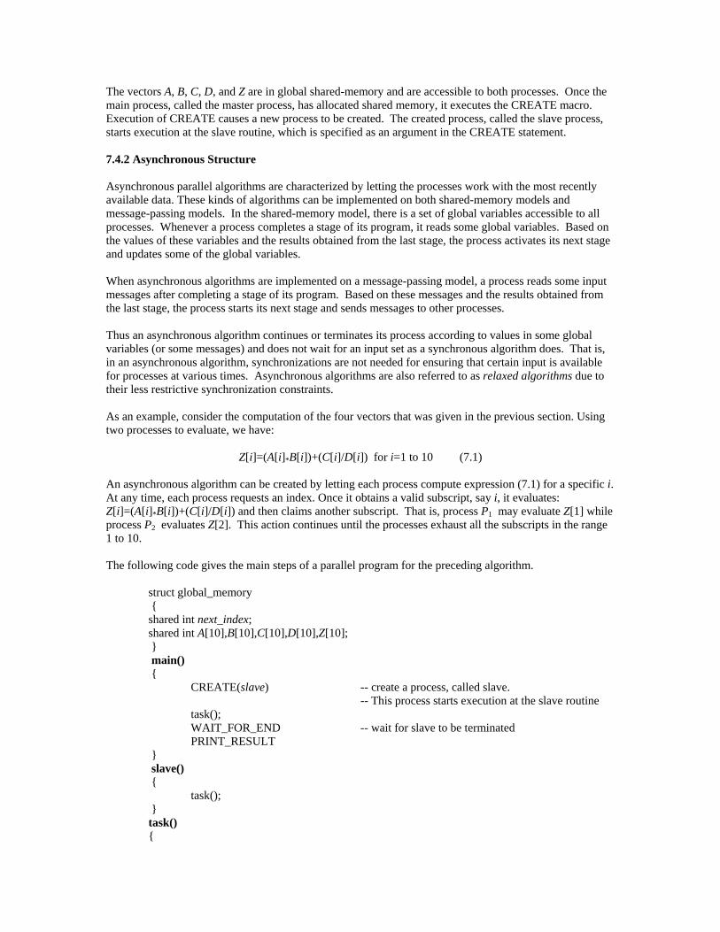
Sometimes we need to copy several data to several processors. For example, assume that there are 64 processors arranged in eight rows. Figure 7.8 represents how the values of a vector, which are stored in the processors of row 0, are duplicated in the other processors. The spreading of the vector to the other processors is done in seven steps. At each step, the values of the ith row of processors (for i=0 to 6) are copied to the (i+1)th row of processors.

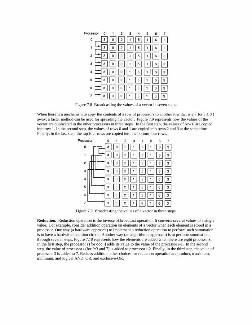
Figure 7.8 Broadcasting the values of a vector in seven steps.

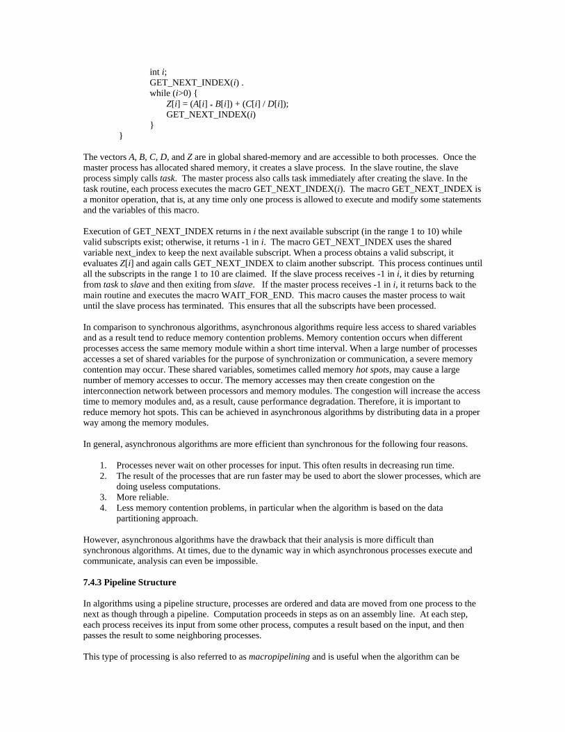
When there is a mechanism to copy the contents of a row of processors to another row that is 2i ( for 0i ) away, a faster method can be used for spreading the vector. Figure 7.9 represents how the values of the vector are duplicated in the other processors in three steps. In the first step, the values of row 0 are copied into row 1. In the second step, the values of rows 0 and 1 are copied into rows 2 and 3 at the same time. Finally, in the last step, the top four rows are copied into the bottom four rows.

Figure 7.9 Broadcasting the values of a vector in three steps.

Reduction. Reduction operation is the inverse of broadcast operation. It converts several values to a single value. For example, consider addition operation on elements of a vector when each element is stored in a processor. One way (a hardware approach) to implement a reduction operation to perform such summation is to have a hardwired addition circuit. Another way (an algorithmic approach) is to perform summation through several steps. Figure 7.10 represents how the elements are added when there are eight processors. In the first step, the processor i (for odd i) adds its value to the value of the processor i-1. In the second step, the value of processor i (for i=3 and 7) is added to processor i-2. Finally, in the third step, the value of processor 3 is added to 7. Besides addition, other choices for reduction operation are product, maximum, minimum, and logical AND, OR, and exclusive-OR.

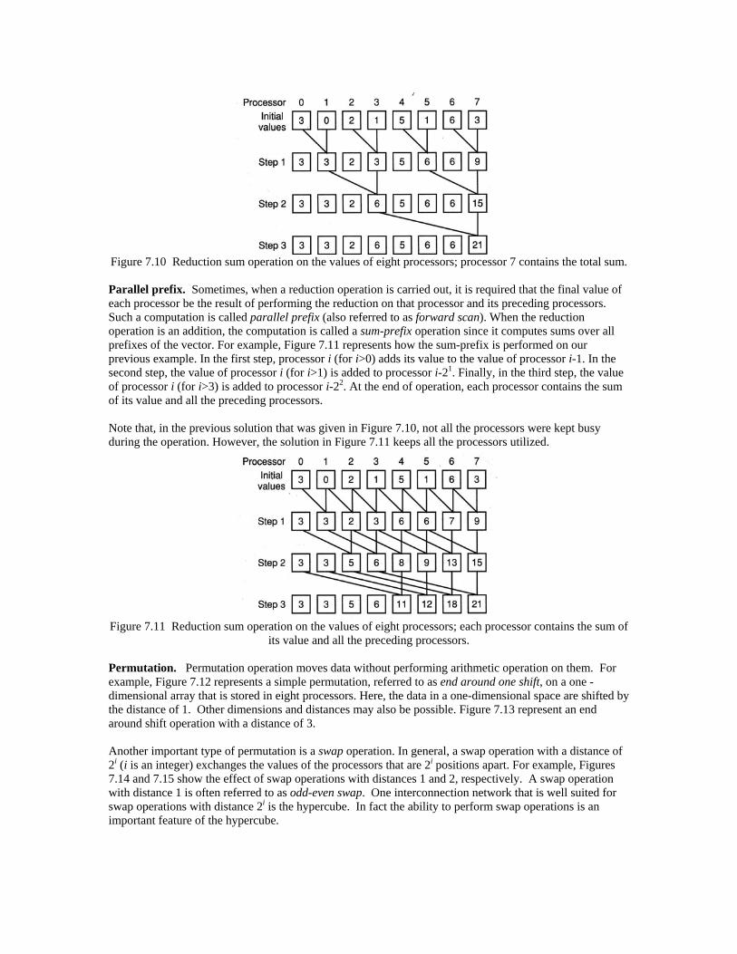
Figure 7.10 Reduction sum operation on the values of eight processors; processor 7 contains the total sum. Parallel prefix. Sometimes, when a reduction operation is carried out, it is required that the final value of each processor be the result of performing the reduction on that processor and its preceding processors. Such a computation is called parallel prefix (also referred to as forward scan). When the reduction operation is an addition, the computation is called a sum-prefix operation since it computes sums over all prefixes of the vector. For example, Figure 7.11 represents how the sum-prefix is performed on our previous example. In the first step, processor i (for i>0) adds its value to the value of processor i-1. In the second step, the value of processor i (for i>1) is added to processor i-21. Finally, in the third step, the value of processor i (for i>3) is added to processor i-22. At the end of operation, each processor contains the sum of its value and all the preceding processors. Note that, in the previous solution that was given in Figure 7.10, not all the processors were kept busy during the operation. However, the solution in Figure 7.11 keeps all the processors utilized.

Figure 7.11 Reduction sum operation on the values of eight processors; each processor contains the sum of

its value and all the preceding processors. Permutation. Permutation operation moves data without performing arithmetic operation on them. For example, Figure 7.12 represents a simple permutation, referred to as end around one shift, on a one -dimensional array that is stored in eight processors. Here, the data in a one-dimensional space are shifted by the distance of 1. Other dimensions and distances may also be possible. Figure 7.13 represent an end around shift operation with a distance of 3. Another important type of permutation is a swap operation. In general, a swap operation with a distance of 2i (i is an integer) exchanges the values of the processors that are 2i positions apart. For example, Figures 7.14 and 7.15 show the effect of swap operations with distances 1 and 2, respectively. A swap operation with distance 1 is often referred to as odd-even swap. One interconnection network that is well suited for swap operations with distance 2i is the hypercube. In fact the ability to perform swap operations is an important feature of the hypercube.

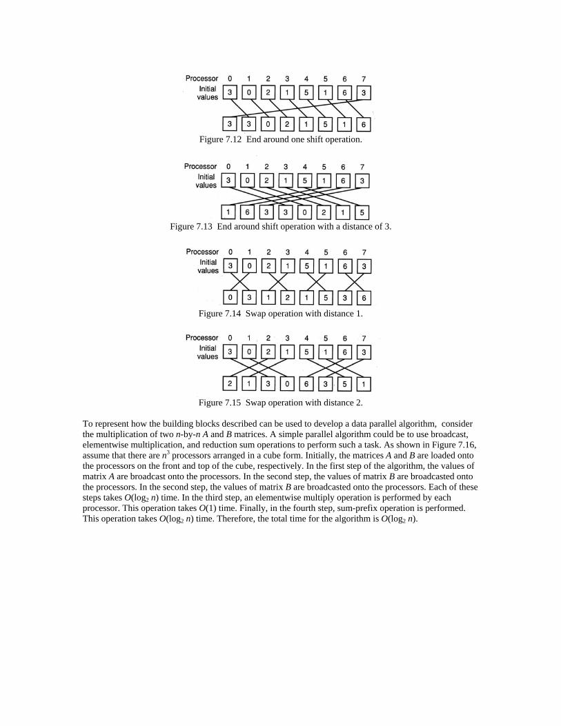
Figure 7.12 End around one shift operation.

Figure 7.13 End around shift operation with a distance of 3.

Figure 7.14 Swap operation with distance 1.

Figure 7.15 Swap operation with distance 2.

To represent how the building blocks described can be used to develop a data parallel algorithm, consider the multiplication of two n-by-n A and B matrices. A simple parallel algorithm could be to use broadcast, elementwise multiplication, and reduction sum operations to perform such a task. As shown in Figure 7.16, assume that there are n3 processors arranged in a cube form. Initially, the matrices A and B are loaded onto the processors on the front and top of the cube, respectively. In the first step of the algorithm, the values of matrix A are broadcast onto the processors. In the second step, the values of matrix B are broadcasted onto the processors. In the second step, the values of matrix B are broadcasted onto the processors. Each of these steps takes O(log2 n) time. In the third step, an elementwise multiply operation is performed by each processor. This operation takes O(1) time. Finally, in the fourth step, sum-prefix operation is performed. This operation takes O(log2 n) time. Therefore, the total time for the algorithm is O(log2 n).

Figure 7.16 Steps of a data parallel algorithm that multiplies two n-by-n A and B matrices. (a) n3 processors arranged in a cube form; A is loaded on the front n2 processors, and B is loaded on the top n2 processors. (b) Broadcasting A. (c) Broadcasting B. (d) Producing C. To clarify the preceding operations, consider A and B to be 2-by-2 matrices defined as: A * B = C

cc

cc

bb

bb

aa

aa

2221

1211

2221

1211

2221

1211

Figure 7.17 represents the value (or values) of each processor for multiplying these two matrices using the preceding steps.

Figure 7.17 Steps of a data parallel algorithm that multiplies two 2-by-2 A and B matrices. (a) Initial values. (b) Broadcasting A. (c) Broadcasting B. (d) Elementwise Multiplications. (e) Parallel sum-prefix.

7.6 ANALYZING PARALLEL ALGORITHMS In a parallel processing environment, efficiency is best measured by run time rather than by processor utilization. In most cases, this is because the goal of parallel processing is to finish the computation as fast as possible, not to efficiently use processors. To make the run time smaller, it seems that a solution would be to increase the number of processes for solving a problem. Although this is true (up to a certain point) for most algorithms, it is not true for all algorithms. In fact, for algorithms that are naturally sequential, their performance may degrade on parallel machines. This is due to the fact that there is the time overhead of creating, synchronizing, and communicating with additional processes. Therefore, these implementation overhead issues should be considered when an algorithm is developed for a parallel machine. To consider the implementation overhead in performance evaluation in general, a measurement, called speedup, is used. Speedup is a measure of how much faster a computation finishes on a parallel machine

than on a uniprocessor machine. The following section explains how this measure is computed. 7.6.1 Speedup One way to evaluate the performance of a parallel algorithm for a problem on a parallel machine is to compare its run time with the run time of the best known sequential algorithm for the same problem on the same (parallel) machine. This comparison, called speedup, is defined as

algorithmparalleltheoftimerun

algorithmsequentialfastesttheoftimerunspeedup

For example, for a given problem, if the best-known sequential algorithm executes in 10 seconds on a single processor, while a parallel algorithm executes in 2 seconds on six processors, a speedup of 5 is achieved for the problem. Sometimes it is hard to obtain the ideal run time of the fastest sequential algorithm for a problem. This may be due to disagreement about the appropriate algorithm or to inefficient implementation of the serial algorithm on a parallel machine. For example, a serial algorithm that requires too much memory may have an inefficient implementation on a parallel machine in which the main memory is divided between the processors. Thus, often the speedup of a parallel algorithm on a parallel machine is obtained by taking the ratio of its run time on one processor to that of a number of processors. If the parallel machine consists of N processors, the maximum speedup that can be achieved is N; this is called perfect speedup. If there is a constant c>0 such that speedup is always cN for any N, the speedup is called linear speedup. Therefore, it is ideal to obtain a linear speedup with c=1. However, in practice many factors degrade this speedup; some of them are the amount of serialization in the program (such as data dependency, loading time of the program, and I/O bottlenecks), synchronization overhead, and communication overhead. In particular, the amount of serialization is considered by Amdahl [AMD 67] as a major deciding factor in speedup. If s represents the execution time (on single processor) of a serial part of a program, and p represents the execution time (on a single processor) of the remainder part of the program that can be done in parallel, then Amdahl's law says that speedup, called fixed-sized speedup, is equal to

Nps

psspeedupsizedfixed

where N is the number of processors. Usually, for algebraic simplicity, the normalized total time, s + p = 1, is used in this expression; thus

Npsspeedupsizedfixed

1

Note in this expression that the speedup can never exceed 1/s no matter how large N is. Thus, Amdahl's law says that the serial parts of a program are an inherent bottleneck blocking speedup. In other words, p (or s = 1-p) is independent of the number of processors. Although this is true when a fixed-sized problem runs on various numbers of processors, it may not be true when the problem size is scaled with the available number of processors. In general, the scaled-sized problem approach is more realistic. This is because, in practice, the number of processors is usually adjusted to the size of the problem in order to keep the run time to a certain desired amount. Gustafson et al. [GUS 88a, GUS 88b] were able to show that (based on some experiments) for some problems the parallel part of a program scales with the problem size, while the serial part does not grow with problem size. That is, when the problem size increases in proportion to the number of processors, s can be decreased by removing the upper bound 1/s for fixed-sized speedup. For example, in [GUS 88b] it is shown that s, which ranges from 0.0006 to 0.001 for some practical fixed-sized problems, can be reduced to a range from 0.000003 to 0.00001 when the problem size is scaled with the number of processors.

Therefore, if s and p represent serial and parallel time spent on N processors (for N>1), rather than a single processor, an alternative to Amdahl's law, called scaled speedup, for scalable problems can be defined as

ps

Npsspeedupscaled

Nps (assuming that s+p=1)

).1( NsN

where s + p*N is the time required for a single processor to perform the program. Cost. The cost of a parallel algorithm is defined as the product of the run time and the number of processors:

cost = run time * number of processors used. As the number of processors increases, the cost also increases. This is because the initial cost and maintenance cost of a parallel machine increases as the number of processors increases. 7.6.2 Factors Affecting Speedup In general, it may not be possible to obtain a perfect (linear) speedup for certain problems. Therefore, the alternative goal is to obtain the best possible speedups for these problems. Several reasons may prevent algorithms from reaching the best possible speedup. Some include algorithm penalty, concurrency, and granularity. Algorithm penalty. This penalty is due to the algorithm being unable to keep the processors busy with work. Overhead costs that cause this penalty are related to distribution, termination, suspension, and synchronization. Distribution overhead is the cost of distributing tasks to processes. Whenever the partitioning of a task is dynamic, some processes may stay idle until they are assigned a task. Termination overhead is the overhead of idle processes at the end of computation. In some algorithms (such as binary addition), as the computation nears completion there will be an increasing number of idle processes. This idle time represents the termination overhead. Suspension overhead is the total time a process is suspended while it waits to be assigned tasks. In general, the suspended overhead serves to show to what extent processes are utilized. The synchronization overhead occurs when some processes, after completing a predetermined part of their task, become idle while waiting for some (or all) of the other processes to reach a similar point of execution in their tasks. Concurrency. The speedup factor is affected by the amount of concurrency in the algorithm. The amount of concurrency is directly affected by the code in the area enclosed by locks. When a section of code is enclosed by locks, only one process can enter. This serves to indirectly synchronize processes by sequentializing those wishing to enter that critical section. As discussed previously, contention for entry into the critical section will arise. (Software lockout is the term used to describe such a condition [QUI 87].) The critical section would then represent a sequential part of the program that affects speedup. Granularity. The performance of an algorithm depends on the program granularity, which refers to the size of the processes. Fine granularity, although providing greater parallelism, leads to greater scheduling and synchronization overhead cost. On the other hand, coarse granularity, although resulting in lower scheduling and synchronization overhead, leads to a significant loss of parallelism. Obviously, both of these situations are undesirable. To achieve high performance, we must extract as much parallelism as

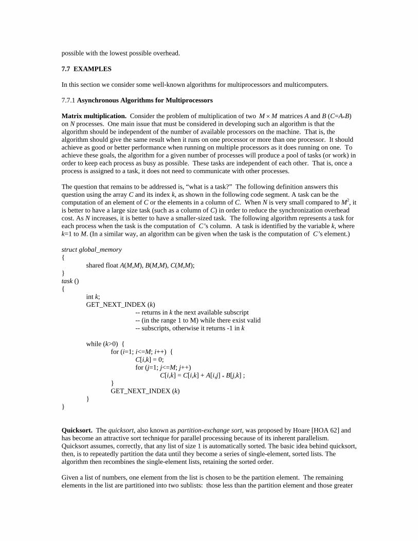
possible with the lowest possible overhead. 7.7 EXAMPLES In this section we consider some well-known algorithms for multiprocessors and multicomputers. 7.7.1 Asynchronous Algorithms for Multiprocessors Matrix multiplication. Consider the problem of multiplication of two MM matrices A and B (C=A*B) on N processes. One main issue that must be considered in developing such an algorithm is that the algorithm should be independent of the number of available processors on the machine. That is, the algorithm should give the same result when it runs on one processor or more than one processor. It should achieve as good or better performance when running on multiple processors as it does running on one. To achieve these goals, the algorithm for a given number of processes will produce a pool of tasks (or work) in order to keep each process as busy as possible. These tasks are independent of each other. That is, once a process is assigned to a task, it does not need to communicate with other processes. The question that remains to be addressed is, “what is a task?” The following definition answers this question using the array C and its index k, as shown in the following code segment. A task can be the computation of an element of C or the elements in a column of C. When N is very small compared to M2, it is better to have a large size task (such as a column of C) in order to reduce the synchronization overhead cost. As N increases, it is better to have a smaller-sized task. The following algorithm represents a task for each process when the task is the computation of C’s column. A task is identified by the variable k, where k=1 to M. (In a similar way, an algorithm can be given when the task is the computation of C’s element.) struct global_memory {

shared float A(M,M), B(M,M), C(M,M); } task () { int k; GET_NEXT_INDEX (k) -- returns in k the next available subscript -- (in the range 1 to M) while there exist valid -- subscripts, otherwise it returns -1 in k while (k>0) { for (i=1; i<=M; i++) { C[i,k] = 0; for (j=1; j<=M; j++) C[i,k] = C[i,k] + A[i,j] * B[j,k] ; } GET_NEXT_INDEX (k) } } Quicksort. The quicksort, also known as partition-exchange sort, was proposed by Hoare [HOA 62] and has become an attractive sort technique for parallel processing because of its inherent parallelism. Quicksort assumes, correctly, that any list of size 1 is automatically sorted. The basic idea behind quicksort, then, is to repeatedly partition the data until they become a series of single-element, sorted lists. The algorithm then recombines the single-element lists, retaining the sorted order. Given a list of numbers, one element from the list is chosen to be the partition element. The remaining elements in the list are partitioned into two sublists: those less than the partition element and those greater

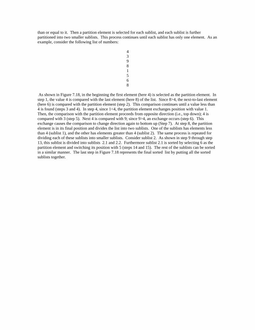
than or equal to it. Then a partition element is selected for each sublist, and each sublist is further partitioned into two smaller sublists. This process continues until each sublist has only one element. As an example, consider the following list of numbers:

4 3 9 8 1 5 6 8

As shown in Figure 7.18, in the beginning the first element (here 4) is selected as the partition element. In step 1, the value 4 is compared with the last element (here 8) of the list. Since 8>4, the next-to-last element (here 6) is compared with the partition element (step 2). This comparison continues until a value less than 4 is found (steps 3 and 4). In step 4, since 1<4, the partition element exchanges position with value 1. Then, the comparison with the partition element proceeds from opposite direction (i.e., top down); 4 is compared with 3 (step 5). Next 4 is compared with 9; since 9>4, an exchange occurs (step 6). This exchange causes the comparison to change direction again to bottom up (Step 7). At step 8, the partition element is in its final position and divides the list into two sublists. One of the sublists has elements less than 4 (sublist 1), and the other has elements greater than 4 (sublist 2). The same process is repeated for dividing each of these sublists into smaller sublists. Consider sublist 2. As shown in step 9 through step 13, this sublist is divided into sublists 2.1 and 2.2. Furthermore sublist 2.1 is sorted by selecting 6 as the partition element and switching its position with 5 (steps 14 and 15). The rest of the sublists can be sorted in a similar manner. The last step in Figure 7.18 represents the final sorted list by putting all the sorted sublists together.

Figure 7.18 Quicksort steps.

One obvious way to implement quicksort in a multiprocessor environment is to create a pool of tasks. Initially, the pool of tasks includes only one task, which is partitioning of the input list. There is a monitor called GET_NEXT_TASK. Each process enters this monitor to find a task to do. One of the processes becomes successful getting the first task (which is the original list) and partitioning it into two sublists. Then it puts one of the sublists into the pool of tasks and repeats the partitioning process for the other sublist. In this way, very soon all the processes become busy by doing some task. When none of the processes can find a task to do, the quicksort ends; at this point the list is sorted. Figure 7.19 presents the task of each process for our quicksort example.

Figure 7.19 Process 1 generates two sublists; one sublist is taken by process 1 and the other is taken by process 2. Furthermore, process 2 partitions the sublist into two sublists; one is taken by itself and the other is taken by process 3. Gaussian elimination. Gaussian elimination is a method used to solve systems of linear equations. For example, Figure 7.20a represents a system with three equations and three unknown variables, x1, x2, and x3. A system of equations can be stored as a matrix. The coefficients of the equations are stored in the matrix, with the constant values on the right side of the equal sign forming the rightmost column of the matrix, as shown in Figure 7.20b. Gaussian elimination consists of two parts, elimination and back substitution. The elimination step converts the matrix into an upper triangular format. A matrix in the upper triangular format is defined such that the kth row of the matrix has zeros in the first k-1th entries, and the kth entry is nonzero. Elimination is performed by starting with the first row and adding a multiple of it to the rows below such that the first column of each of the remaining rows becomes zero. In Figure 7.20c, the multiplier value to be used for the first row when it is added to the second row is -a(2,1)/a(1,1) = -2. This process is repeated for all of the successive rows in turn except the last, resulting in Figure 7.20d. The selected row that is added to the other rows is called the pivot row. The preceding process is called Gaussian elimination without interchanges; alternatively, if the matrix has zero in the kth element of the pivot row, the rows need to be swapped for the method to work. This is known as Gaussian elimination with interchanges. The Gaussian elimination with interchanges chooses the unpivoted row with the largest element in the currently selected column. If this row is not the pivot row, it is swapped to become the new pivot row. The example has no zero elements, so it uses the method without interchanges. When the matrix is in upper triangular format, back substitution is used to solve for the unknown variables. Starting at the bottom row and working upward, the variables are solved one at a time and then substituted in the rows above (see Figure 7.20e).

x1+2x2-x3=-7 2x1-x2+x3=7 -x1+2x2+3x3=-1

(a)

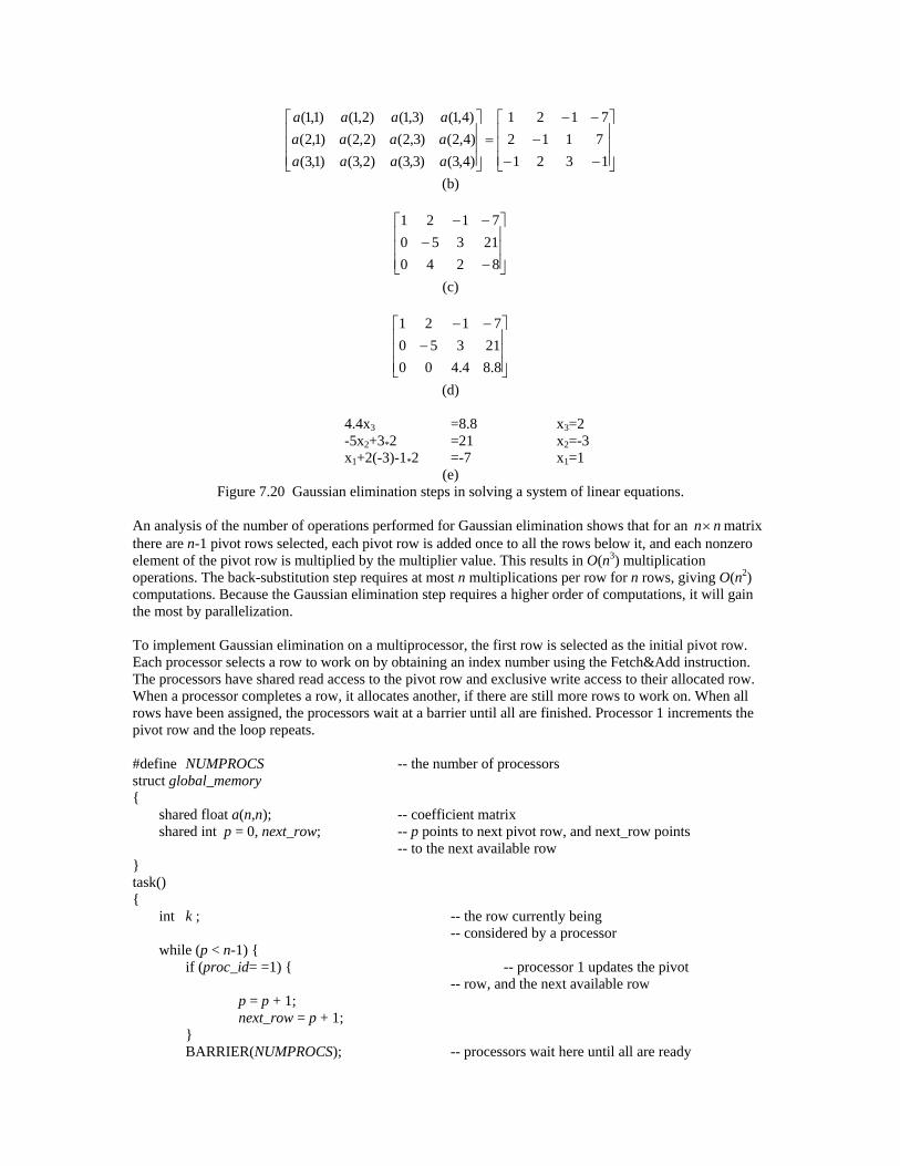
1

7

7

3

1

1

2

1

2

1

2

1

)4,3(

)4,2(

)4,1(

)3,3(

)3,2(

)3,1(

)2,3(

)2,2(

)2,1(

)1,3(

)1,2(

)1,1(

a

a

a

a

a

a

a

a

a

a

a

a

(b)

8

21

7

2

3

1

4

5

2

0

0

1

(c)

8.8

21

7

4.4

3

1

0

5

2

0

0

1

(d)

4.4x3 =8.8 x3=2 -5x2+3*2 =21 x2=-3 x1+2(-3)-1*2 =-7 x1=1

(e) Figure 7.20 Gaussian elimination steps in solving a system of linear equations.

An analysis of the number of operations performed for Gaussian elimination shows that for an nn matrix there are n-1 pivot rows selected, each pivot row is added once to all the rows below it, and each nonzero element of the pivot row is multiplied by the multiplier value. This results in O(n3) multiplication operations. The back-substitution step requires at most n multiplications per row for n rows, giving O(n2) computations. Because the Gaussian elimination step requires a higher order of computations, it will gain the most by parallelization. To implement Gaussian elimination on a multiprocessor, the first row is selected as the initial pivot row. Each processor selects a row to work on by obtaining an index number using the Fetch&Add instruction. The processors have shared read access to the pivot row and exclusive write access to their allocated row. When a processor completes a row, it allocates another, if there are still more rows to work on. When all rows have been assigned, the processors wait at a barrier until all are finished. Processor 1 increments the pivot row and the loop repeats. #define NUMPROCS -- the number of processors struct global_memory {

shared float a(n,n); -- coefficient matrix shared int p = 0, next_row; -- p points to next pivot row, and next_row points

-- to the next available row } task() {

int k ; -- the row currently being -- considered by a processor while (p < n-1) { if (proc_id= =1) { -- processor 1 updates the pivot -- row, and the next available row p = p + 1; next_row = p + 1; } BARRIER(NUMPROCS); -- processors wait here until all are ready

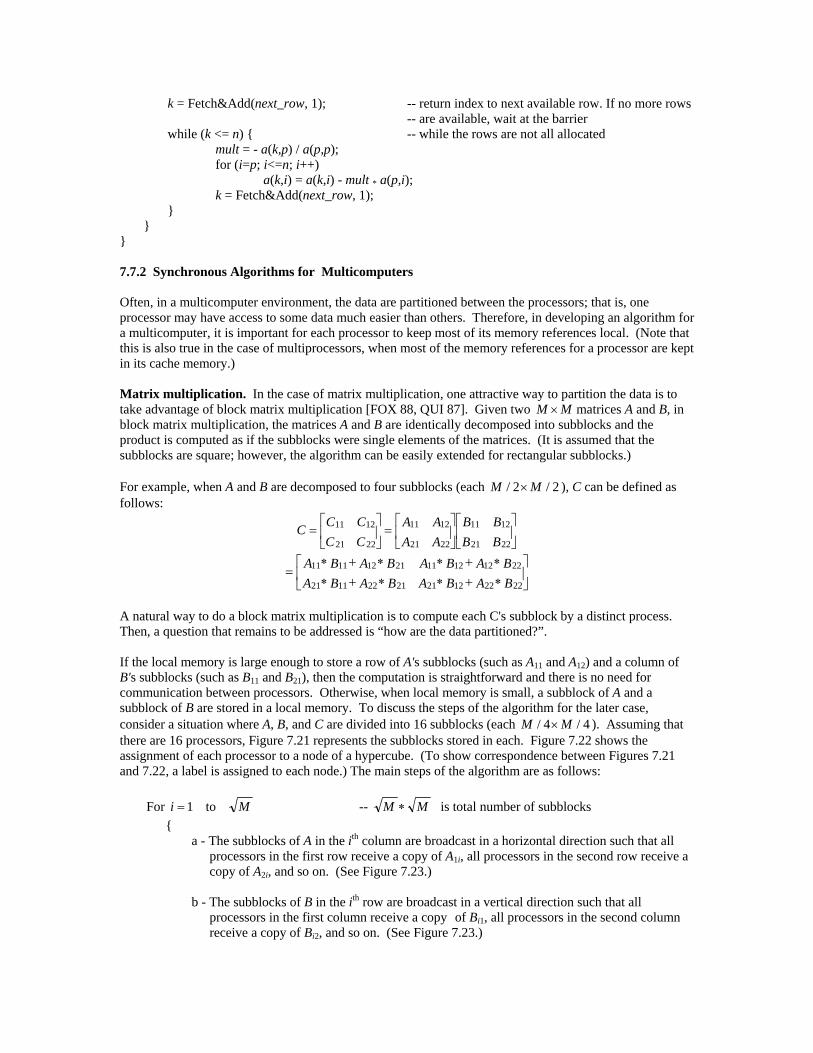
k = Fetch&Add(next_row, 1); -- return index to next available row. If no more rows -- are available, wait at the barrier while (k <= n) { -- while the rows are not all allocated mult = - a(k,p) / a(p,p); for (i=p; i<=n; i++) a(k,i) = a(k,i) - mult * a(p,i); k = Fetch&Add(next_row, 1); } }

} 7.7.2 Synchronous Algorithms for Multicomputers Often, in a multicomputer environment, the data are partitioned between the processors; that is, one processor may have access to some data much easier than others. Therefore, in developing an algorithm for a multicomputer, it is important for each processor to keep most of its memory references local. (Note that this is also true in the case of multiprocessors, when most of the memory references for a processor are kept in its cache memory.) Matrix multiplication. In the case of matrix multiplication, one attractive way to partition the data is to take advantage of block matrix multiplication [FOX 88, QUI 87]. Given two MM matrices A and B, in block matrix multiplication, the matrices A and B are identically decomposed into subblocks and the product is computed as if the subblocks were single elements of the matrices. (It is assumed that the subblocks are square; however, the algorithm can be easily extended for rectangular subblocks.) For example, when A and B are decomposed to four subblocks (each 2/2/ MM ), C can be defined as follows:

BB

BB

AA

AA

CC

CCC

2221

1211

2221

1211

2221

1211

BABABABA

BABABABA

2222122121221121

2212121121121111

A natural way to do a block matrix multiplication is to compute each C's subblock by a distinct process. Then, a question that remains to be addressed is “how are the data partitioned?”. If the local memory is large enough to store a row of A's subblocks (such as A11 and A12) and a column of B's subblocks (such as B11 and B21), then the computation is straightforward and there is no need for communication between processors. Otherwise, when local memory is small, a subblock of A and a subblock of B are stored in a local memory. To discuss the steps of the algorithm for the later case, consider a situation where A, B, and C are divided into 16 subblocks (each 4/4/ MM ). Assuming that there are 16 processors, Figure 7.21 represents the subblocks stored in each. Figure 7.22 shows the assignment of each processor to a node of a hypercube. (To show correspondence between Figures 7.21 and 7.22, a label is assigned to each node.) The main steps of the algorithm are as follows:

For Mi to1 -- MM is total number of subblocks

{ a - The subblocks of A in the ith column are broadcast in a horizontal direction such that all

processors in the first row receive a copy of A1i, all processors in the second row receive a copy of A2i, and so on. (See Figure 7.23.)

b - The subblocks of B in the ith row are broadcast in a vertical direction such that all

processors in the first column receive a copy of Bi1, all processors in the second column receive a copy of Bi2, and so on. (See Figure 7.23.)

c - The broadcast of A subblocks is multiplied by the broadcast of B subblocks and the results are added to the partial results in the subblock of C. (See Figure 7.23.)

}

Figure 7.21 Stored blocks in each local memory.

Figure 7.22 Assigned block to the nodes of a 4-cube Multicomputer.

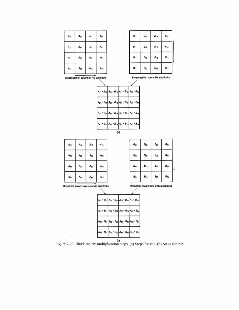
Figure 7.23 Block matrix multiplication steps. (a) Steps for i=1. (b) Steps for i=2.