511 Basics Handouts
13
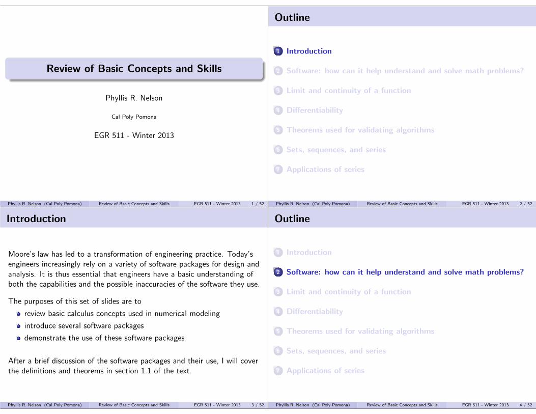
Review of Basic Concepts and Skills Phyllis R. Nelson Cal Poly Pomona EGR 511 - Winter 2013 Phyllis R. Nelson (Cal Poly Pomona) Review of Basic Concepts and Skills EGR 511 - Winter 2013 1 / 52 Outline 1 Introduction 2 Software: how can it help understand and solve math problems? 3 Limit and continuity of a function 4 Differentiability 5 Theorems used for validating algorithms 6 Sets, sequences, and series 7 Applications of series Phyllis R. Nelson (Cal Poly Pomona) Review of Basic Concepts and Skills EGR 511 - Winter 2013 2 / 52 Introduction Moore’s law has led to a transformation of engineering practice. Today’s engineers increasingly rely on a variety of software packages for design and analysis. It is thus essential that engineers have a basic understanding of both the capabilities and the possible inaccuracies of the software they use. The purposes of this set of slides are to review basic calculus concepts used in numerical modeling introduce several software packages demonstrate the use of these software packages After a brief discussion of the software packages and their use, I will cover the definitions and theorems in section 1.1 of the text. Phyllis R. Nelson (Cal Poly Pomona) Review of Basic Concepts and Skills EGR 511 - Winter 2013 3 / 52 Outline 1 Introduction 2 Software: how can it help understand and solve math problems? 3 Limit and continuity of a function 4 Differentiability 5 Theorems used for validating algorithms 6 Sets, sequences, and series 7 Applications of series Phyllis R. Nelson (Cal Poly Pomona) Review of Basic Concepts and Skills EGR 511 - Winter 2013 4 / 52
Transcript of 511 Basics Handouts
Review of Basic Concepts and Skills
Phyllis R. Nelson
Cal Poly Pomona
EGR 511 - Winter 2013
Phyllis R. Nelson (Cal Poly Pomona) Review of Basic Concepts and Skills EGR 511 - Winter 2013 1 / 52
Outline
1 Introduction
2 Software: how can it help understand and solve math problems?
3 Limit and continuity of a function
4 Differentiability
5 Theorems used for validating algorithms
6 Sets, sequences, and series
7 Applications of series
Phyllis R. Nelson (Cal Poly Pomona) Review of Basic Concepts and Skills EGR 511 - Winter 2013 2 / 52
Introduction
Moore’s law has led to a transformation of engineering practice. Today’sengineers increasingly rely on a variety of software packages for design andanalysis. It is thus essential that engineers have a basic understanding ofboth the capabilities and the possible inaccuracies of the software they use.
The purposes of this set of slides are to
review basic calculus concepts used in numerical modeling
introduce several software packages
demonstrate the use of these software packages
After a brief discussion of the software packages and their use, I will coverthe definitions and theorems in section 1.1 of the text.
Phyllis R. Nelson (Cal Poly Pomona) Review of Basic Concepts and Skills EGR 511 - Winter 2013 3 / 52
Outline
1 Introduction
2 Software: how can it help understand and solve math problems?
3 Limit and continuity of a function
4 Differentiability
5 Theorems used for validating algorithms
6 Sets, sequences, and series
7 Applications of series
Phyllis R. Nelson (Cal Poly Pomona) Review of Basic Concepts and Skills EGR 511 - Winter 2013 4 / 52
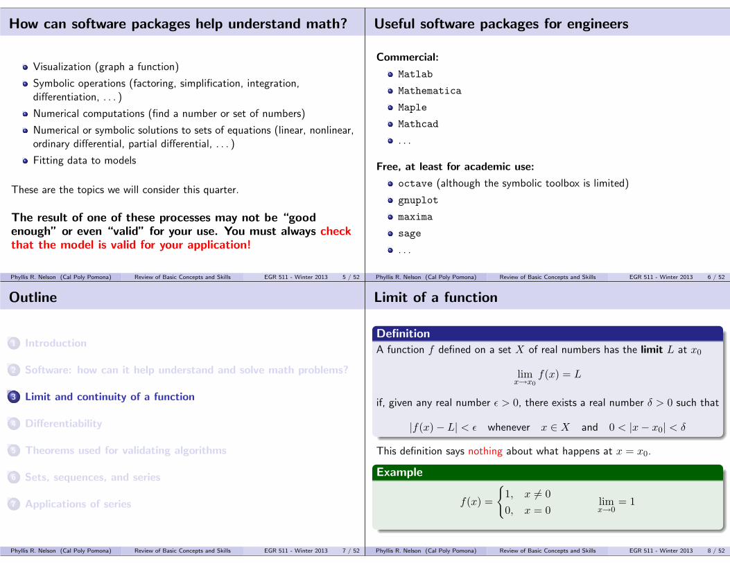
How can software packages help understand math?
Visualization (graph a function)
Symbolic operations (factoring, simplification, integration,differentiation, . . . )
Numerical computations (find a number or set of numbers)
Numerical or symbolic solutions to sets of equations (linear, nonlinear,ordinary differential, partial differential, . . . )
Fitting data to models
These are the topics we will consider this quarter.
The result of one of these processes may not be “goodenough” or even “valid” for your use. You must always checkthat the model is valid for your application!
Phyllis R. Nelson (Cal Poly Pomona) Review of Basic Concepts and Skills EGR 511 - Winter 2013 5 / 52
Useful software packages for engineers
Commercial:
Matlab
Mathematica
Maple
Mathcad
. . .
Free, at least for academic use:
octave (although the symbolic toolbox is limited)
gnuplot
maxima
sage
. . .
Phyllis R. Nelson (Cal Poly Pomona) Review of Basic Concepts and Skills EGR 511 - Winter 2013 6 / 52
Outline
1 Introduction
2 Software: how can it help understand and solve math problems?
3 Limit and continuity of a function
4 Differentiability
5 Theorems used for validating algorithms
6 Sets, sequences, and series
7 Applications of series
Phyllis R. Nelson (Cal Poly Pomona) Review of Basic Concepts and Skills EGR 511 - Winter 2013 7 / 52
Limit of a function
Definition
A function f defined on a set X of real numbers has the limit L at x0
limx→x0
f(x) = L
if, given any real number ε > 0, there exists a real number δ > 0 such that
|f(x)− L| < ε whenever x ∈ X and 0 < |x− x0| < δ
This definition says nothing about what happens at x = x0.
Example
f(x) =
{1, x 6= 00, x = 0
limx→0
= 1
Phyllis R. Nelson (Cal Poly Pomona) Review of Basic Concepts and Skills EGR 511 - Winter 2013 8 / 52

Limits involving infinity
Definition
A function f defined on a set of real numbers has the limit ∞ at x0
limx→x0
f(x) =∞
if, given any real number ε > 0, there exists a real number δ > 0 such that
f(x) > ε whenever x ∈ X and 0 < |x− x0| < δ
A similar definition can be constructed for a limit of −∞.
Example
limx→0
x−2 =∞ limx→±1
x2 + 2x2 − 1
do not exist
Phyllis R. Nelson (Cal Poly Pomona) Review of Basic Concepts and Skills EGR 511 - Winter 2013 9 / 52
Limits involving infinity - (2)
Example
limx→±1
x2 + 2x2 − 1
Visualization:Use gnuplot to plot this function near x = ±1.
set xrange [-5:5]set yrange [-25:25]plot (x**2+2)/(x**2-1), 0
The left and right limits atx = ±1 are ±∞, so thereis no unique value L.
Phyllis R. Nelson (Cal Poly Pomona) Review of Basic Concepts and Skills EGR 511 - Winter 2013 10 / 52
Limits involving infinity - (3)
Definition
A function f defined on a set of real numbers that includes ∞ has thelimit L as x→∞
limx→∞ f(x) = L
if, given any real number ε > 0, there exists a real number δ > 0 such that
|f(x)− L| < ε whenever x ∈ X and x > δ
Example
limx→∞ e
−x = 0 limx→∞ a−
1x+ a
= a
Phyllis R. Nelson (Cal Poly Pomona) Review of Basic Concepts and Skills EGR 511 - Winter 2013 11 / 52
Continuity of a function
Definition
Let f be a function defined on a set X of real numbers and x0 ∈ X. Thenf is continuous at x0 if
limx→x0
f(x) = f(x0)
The function f is continuous on the set X if it is continuous at eachnumber in X.
Example
At x = 0, f(x) and g(x) have removable singularities.
f(x) =
{1, x 6= 00, x = 0
g(x) =sinxx
h(x) = x−1
Phyllis R. Nelson (Cal Poly Pomona) Review of Basic Concepts and Skills EGR 511 - Winter 2013 12 / 52
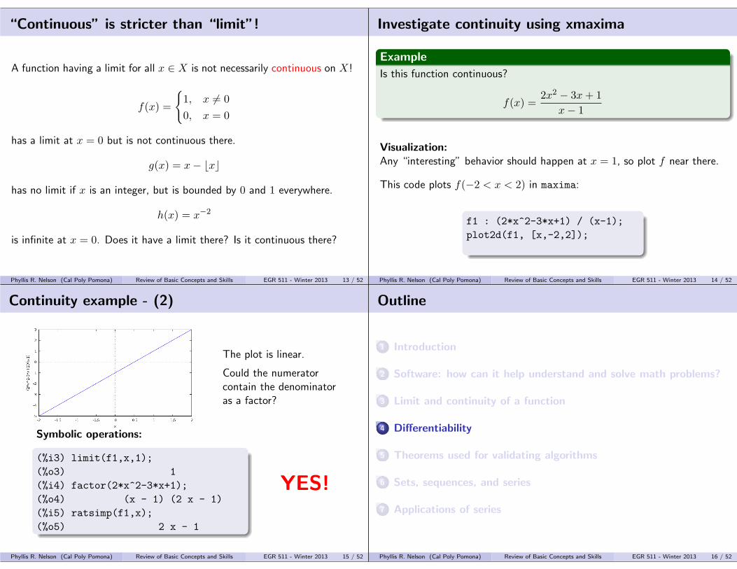
“Continuous” is stricter than “limit”!
A function having a limit for all x ∈ X is not necessarily continuous on X!
f(x) =
{1, x 6= 00, x = 0
has a limit at x = 0 but is not continuous there.
g(x) = x− bxc
has no limit if x is an integer, but is bounded by 0 and 1 everywhere.
h(x) = x−2
is infinite at x = 0. Does it have a limit there? Is it continuous there?
Phyllis R. Nelson (Cal Poly Pomona) Review of Basic Concepts and Skills EGR 511 - Winter 2013 13 / 52
Investigate continuity using xmaxima
Example
Is this function continuous?
f(x) =2x2 − 3x+ 1
x− 1
Visualization:Any “interesting” behavior should happen at x = 1, so plot f near there.
This code plots f(−2 < x < 2) in maxima:
f1 : (2*x^2-3*x+1) / (x-1);plot2d(f1, [x,-2,2]);
Phyllis R. Nelson (Cal Poly Pomona) Review of Basic Concepts and Skills EGR 511 - Winter 2013 14 / 52
Continuity example - (2)
The plot is linear.
Could the numeratorcontain the denominatoras a factor?
Symbolic operations:
(%i3) limit(f1,x,1);(%o3) 1(%i4) factor(2*x^2-3*x+1);(%o4) (x - 1) (2 x - 1)(%i5) ratsimp(f1,x);(%o5) 2 x - 1
YES!
Phyllis R. Nelson (Cal Poly Pomona) Review of Basic Concepts and Skills EGR 511 - Winter 2013 15 / 52
Outline
1 Introduction
2 Software: how can it help understand and solve math problems?
3 Limit and continuity of a function
4 Differentiability
5 Theorems used for validating algorithms
6 Sets, sequences, and series
7 Applications of series
Phyllis R. Nelson (Cal Poly Pomona) Review of Basic Concepts and Skills EGR 511 - Winter 2013 16 / 52

Differentiability
Definition
The function f , which is defined in an open interval containing x0, isdifferentiable and has a derivative f ′ at x0 if the following limit exists:
f ′(x0) = limx→x0
f(x)− f(x0)x− x0
A function having a derivative at each x ∈ X is differentiable on X.
The derivative f ′(x0) gives the slope of the curve f(x) at x = x0. Thus,the line through the point (x0, f(x0)) with slope f ′(x0) is the tangent tothe curve of f(x) vs. x at x = x0.
Phyllis R. Nelson (Cal Poly Pomona) Review of Basic Concepts and Skills EGR 511 - Winter 2013 17 / 52
Investigate differentiability
Example
f(x) = |x| =
x x > 00 x = 0−x x < 0
f ′(x) is 1 for x > 0 and −1 forx < 0, but does not exist at x = 0.
Phyllis R. Nelson (Cal Poly Pomona) Review of Basic Concepts and Skills EGR 511 - Winter 2013 18 / 52
Outline
1 Introduction
2 Software: how can it help understand and solve math problems?
3 Limit and continuity of a function
4 Differentiability
5 Theorems used for validating algorithms
6 Sets, sequences, and series
7 Applications of series
Phyllis R. Nelson (Cal Poly Pomona) Review of Basic Concepts and Skills EGR 511 - Winter 2013 19 / 52
Rolle’s theorem
Theorem
Suppose f ∈ C[a, b] and f is differentiable on (a, b). If f(a) = f(b), thena number c in (a, b) exists with f ′(c) = 0.
Example
Rolle’s theorem applies for
f(x) = x(x2 − 1) g(x) =√
1− x2 both for x ∈ [−1, 1]
f is continuous and differentiable everywhere, while g is only real forx ∈ [−1, 1] and is not differentiable at x = ±1.
Example
Rolle’s theorem can’t be used for f(x) = |x| if (a, b) includes 0. (Why?)
Phyllis R. Nelson (Cal Poly Pomona) Review of Basic Concepts and Skills EGR 511 - Winter 2013 20 / 52

Investigate Rolle’s theorem using xmaxima
plot2d(x*(x^2-1),[x,-1,1]);
f ′(x) = 3x2 − 1 = 0
at x = ± 1√3
plot2d(sqrt(1-x^2),[x,-1,1]);
g′(x) = − x√1− x2
= 0
at x = 0
Phyllis R. Nelson (Cal Poly Pomona) Review of Basic Concepts and Skills EGR 511 - Winter 2013 21 / 52
Mean value theorem
Theorem
If f ∈ C[a, b] and f is differentiable on (a, b), then a number c in (a, b)exists with
f ′(c) =f(b)− f(a)
b− a
Example
f(x) =√
1− x2 − x
plot2d([sqrt(1-x^2)-x,1-x,-x],[x,-1,1]);
Phyllis R. Nelson (Cal Poly Pomona) Review of Basic Concepts and Skills EGR 511 - Winter 2013 22 / 52
Extreme value theorem
Theorem
If f ∈ C[a, b] then c1, c2 ∈ [a, b] exist with f(c1) ≤ f(x) ≤ f(c2) for allx ∈ [a, b].
If f is differentiable on (a, b), then the numbers c1 and c2 occur either atthe endpoints of [a, b] or where f ′ is zero.
Example
f(x) =√
1− x2 − x
f ′(x) = − x√1− x2
−1
f ′(x) = 0 ⇒ x = − 1√2
plot2d([sqrt(1-x^2)-x],[x,-1,1]);
Phyllis R. Nelson (Cal Poly Pomona) Review of Basic Concepts and Skills EGR 511 - Winter 2013 23 / 52
Generalized Rolle’s theorem
Theorem
Suppose f ∈ C[a, b] is n times differentiable on (a, b). If f(x) = 0 at then+ 1 distinct numbers a ≤ x0 < x1 < . . . < xn ≤ b, then a number c in(x0, xn), and hence in (a, b), exists with f (n)(c) = 0.
This theorem is seldom used excedpt in proofs. I will skip it.
Phyllis R. Nelson (Cal Poly Pomona) Review of Basic Concepts and Skills EGR 511 - Winter 2013 24 / 52
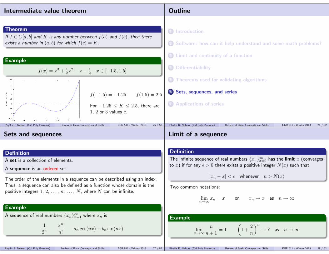
Intermediate value theorem
Theorem
If f ∈ C[a, b] and K is any number between f(a) and f(b), then thereexists a number in (a, b) for which f(c) = K.
Example
f(x) = x3 + 12x
2 − x− 12 x ∈ [−1.5, 1.5]
f(−1.5) = −1.25 f(1.5) = 2.5
For −1.25 ≤ K ≤ 2.5, there are1, 2 or 3 values c.
Phyllis R. Nelson (Cal Poly Pomona) Review of Basic Concepts and Skills EGR 511 - Winter 2013 25 / 52
Outline
1 Introduction
2 Software: how can it help understand and solve math problems?
3 Limit and continuity of a function
4 Differentiability
5 Theorems used for validating algorithms
6 Sets, sequences, and series
7 Applications of series
Phyllis R. Nelson (Cal Poly Pomona) Review of Basic Concepts and Skills EGR 511 - Winter 2013 26 / 52
Sets and sequences
Definition
A set is a collection of elements.
A sequence is an ordered set.
The order of the elements in a sequence can be described using an index.Thus, a sequence can also be defined as a function whose domain is thepositive integers 1, 2, . . . , n, . . . , N , where N can be infinite.
Example
A sequence of real numbers {xn}∞n=1 where xn is
12n
xn
n!an cos(nx) + bn sin(nx)
Phyllis R. Nelson (Cal Poly Pomona) Review of Basic Concepts and Skills EGR 511 - Winter 2013 27 / 52
Limit of a sequence
Definition
The infinite sequence of real numbers {xn}∞x=0 has the limit x (convergesto x) if for any ε > 0 there exists a positive integer N(x) such that
|xn − x| < ε whenever n > N(x)
Two common notations:
limn→∞xn = x or xn → x as n→∞
Example
limn→∞
n
n+ 1= 1
(1 +
2n
)n→ ? as n→∞
Phyllis R. Nelson (Cal Poly Pomona) Review of Basic Concepts and Skills EGR 511 - Winter 2013 28 / 52

Investigate a sequence using Matlab (octave)
Example (1 +
2n
)n→ ? as n→∞
Visualization:
This time we want to plot individual points, not a continuous curve.Here’s the octave code and resulting plot:
t = 1:1:25;plot((1.+2./t).^t,’x’);
There is a (finite) limit.
e2 ' 7.3891Phyllis R. Nelson (Cal Poly Pomona) Review of Basic Concepts and Skills EGR 511 - Winter 2013 29 / 52
Series
Definition
Given a sequence of real or complex numbers {xn}, generate the sequence{sn} of the partial sums of {xn}
sn =n∑k=1
xn
The sequence {sn} is a series and its limit as n→∞ is called the sum.
Example
{xn} =1
2n−1{sn} =
n∑k=1
12k−1
Phyllis R. Nelson (Cal Poly Pomona) Review of Basic Concepts and Skills EGR 511 - Winter 2013 30 / 52
Investigate a series
{xn} =1
2n−1
In octave
n = 1:1:10;x = 1./2.^(n.-1);plot(n,x,’x’);
The value of xn approaches 0 as n increases, so it is possible that theseries of partial sums converges.
Phyllis R. Nelson (Cal Poly Pomona) Review of Basic Concepts and Skills EGR 511 - Winter 2013 31 / 52
Series example - (2)
{sn} =n∑k=1
12k−1
s = zeros(1,10);s(1) = x(1);for i=2:length(n)s(i) = s(i-1) + x(i);
endfor;plot(n,s,’x’);
The sum of the series appears to be 2 (s(10) = 1.9980). How could weconfirm that?
What happens if the 2 in the sequence definition is replaced by some othernumber? Clearly that number must be > 1 if the series is to converge.(Why?)
Phyllis R. Nelson (Cal Poly Pomona) Review of Basic Concepts and Skills EGR 511 - Winter 2013 32 / 52
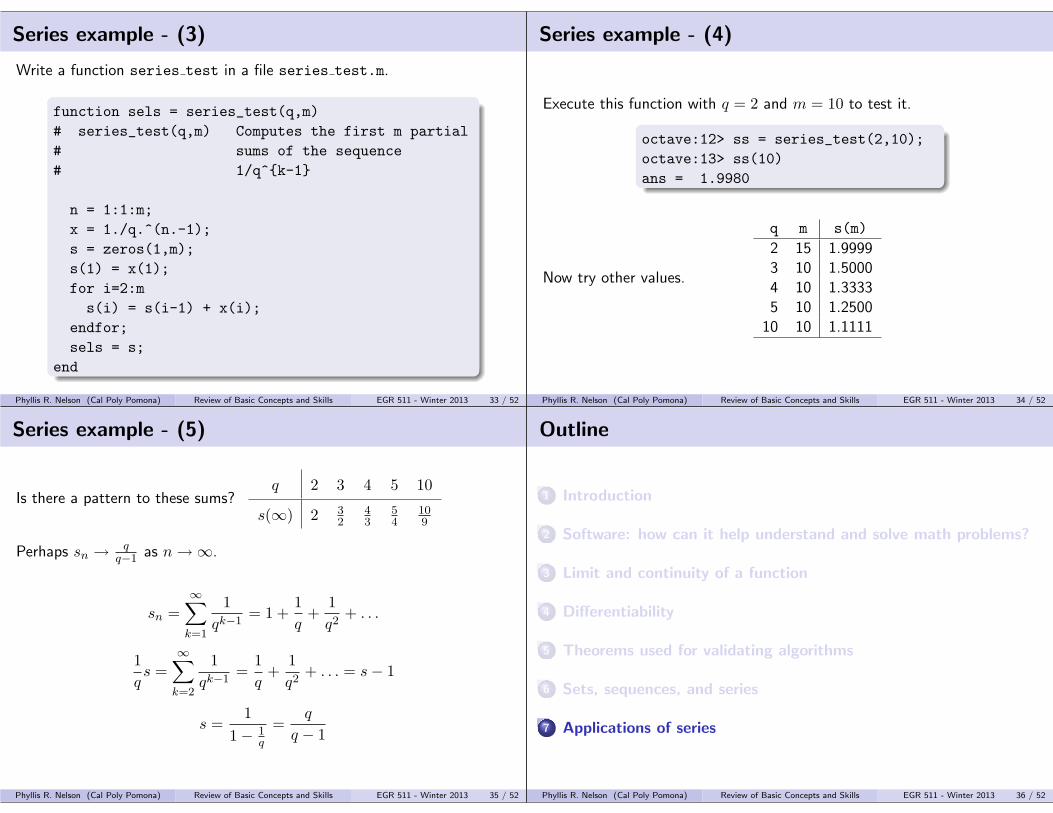
Series example - (3)
Write a function series test in a file series test.m.
function sels = series_test(q,m)# series_test(q,m) Computes the first m partial# sums of the sequence# 1/q^{k-1}
n = 1:1:m;x = 1./q.^(n.-1);s = zeros(1,m);s(1) = x(1);for i=2:ms(i) = s(i-1) + x(i);
endfor;sels = s;
end
Phyllis R. Nelson (Cal Poly Pomona) Review of Basic Concepts and Skills EGR 511 - Winter 2013 33 / 52
Series example - (4)
Execute this function with q = 2 and m = 10 to test it.
octave:12> ss = series_test(2,10);octave:13> ss(10)ans = 1.9980
Now try other values.
q m s(m)2 15 1.99993 10 1.50004 10 1.33335 10 1.2500
10 10 1.1111
Phyllis R. Nelson (Cal Poly Pomona) Review of Basic Concepts and Skills EGR 511 - Winter 2013 34 / 52
Series example - (5)
Is there a pattern to these sums?q 2 3 4 5 10
s(∞) 2 32
43
54
109
Perhaps sn → qq−1 as n→∞.
sn =∞∑k=1
1qk−1
= 1 +1q
+1q2
+ . . .
1qs =
∞∑k=2
1qk−1
=1q
+1q2
+ . . . = s− 1
s =1
1− 1q
=q
q − 1
Phyllis R. Nelson (Cal Poly Pomona) Review of Basic Concepts and Skills EGR 511 - Winter 2013 35 / 52
Outline
1 Introduction
2 Software: how can it help understand and solve math problems?
3 Limit and continuity of a function
4 Differentiability
5 Theorems used for validating algorithms
6 Sets, sequences, and series
7 Applications of series
Phyllis R. Nelson (Cal Poly Pomona) Review of Basic Concepts and Skills EGR 511 - Winter 2013 36 / 52
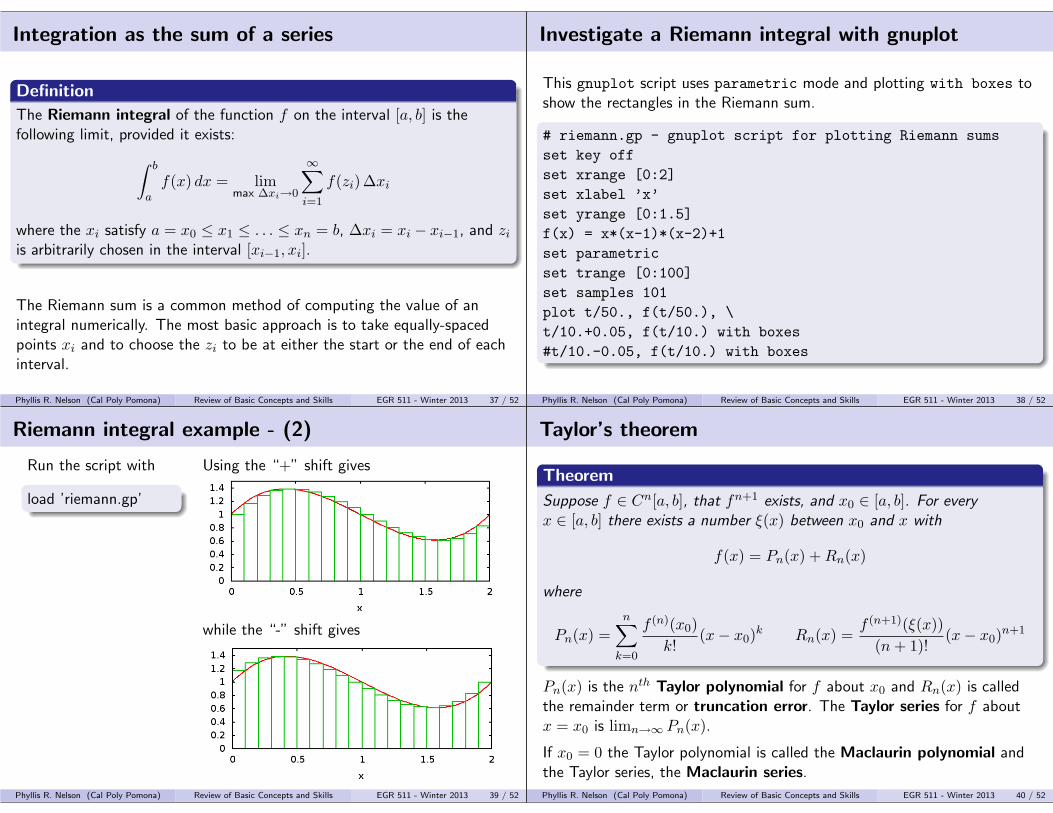
Integration as the sum of a series
Definition
The Riemann integral of the function f on the interval [a, b] is thefollowing limit, provided it exists:∫ b
af(x) dx = lim
max ∆xi→0
∞∑i=1
f(zi) ∆xi
where the xi satisfy a = x0 ≤ x1 ≤ . . . ≤ xn = b, ∆xi = xi − xi−1, and ziis arbitrarily chosen in the interval [xi−1, xi].
The Riemann sum is a common method of computing the value of anintegral numerically. The most basic approach is to take equally-spacedpoints xi and to choose the zi to be at either the start or the end of eachinterval.
Phyllis R. Nelson (Cal Poly Pomona) Review of Basic Concepts and Skills EGR 511 - Winter 2013 37 / 52
Investigate a Riemann integral with gnuplot
This gnuplot script uses parametric mode and plotting with boxes toshow the rectangles in the Riemann sum.
# riemann.gp - gnuplot script for plotting Riemann sumsset key offset xrange [0:2]set xlabel ’x’set yrange [0:1.5]f(x) = x*(x-1)*(x-2)+1set parametricset trange [0:100]set samples 101plot t/50., f(t/50.), \t/10.+0.05, f(t/10.) with boxes#t/10.-0.05, f(t/10.) with boxes
Phyllis R. Nelson (Cal Poly Pomona) Review of Basic Concepts and Skills EGR 511 - Winter 2013 38 / 52
Riemann integral example - (2)
Run the script with
load ’riemann.gp’
Using the “+” shift gives
while the “-” shift gives
Phyllis R. Nelson (Cal Poly Pomona) Review of Basic Concepts and Skills EGR 511 - Winter 2013 39 / 52
Taylor’s theorem
Theorem
Suppose f ∈ Cn[a, b], that fn+1 exists, and x0 ∈ [a, b]. For everyx ∈ [a, b] there exists a number ξ(x) between x0 and x with
f(x) = Pn(x) +Rn(x)
where
Pn(x) =n∑k=0
f (n)(x0)k!
(x− x0)k Rn(x) =f (n+1)(ξ(x))
(n+ 1)!(x− x0)n+1
Pn(x) is the nth Taylor polynomial for f about x0 and Rn(x) is calledthe remainder term or truncation error. The Taylor series for f aboutx = x0 is limn→∞ Pn(x).
If x0 = 0 the Taylor polynomial is called the Maclaurin polynomial andthe Taylor series, the Maclaurin series.
Phyllis R. Nelson (Cal Poly Pomona) Review of Basic Concepts and Skills EGR 511 - Winter 2013 40 / 52

Approximate a function with a Taylor polynomial
The third Taylor polynomial for f(x) = tanx about x0 = 0 is
P3(x) = f(0) + f ′(0)x+f ′′(0)
2!x2 +
f (3)(0)3!
x3
f(0) = tan(x)|x=0 = 0 f ′(0) = sec2 x∣∣x=0
= 1
f ′′(0) = 2 sec2 x tanx∣∣x=0
= 0
f (3)(0) =[4 sec2 x tanx+ 2 sec4 x
]x=0
= 2
P3(x) = x+x3
3
Phyllis R. Nelson (Cal Poly Pomona) Review of Basic Concepts and Skills EGR 511 - Winter 2013 41 / 52
Taylor polynomial approximation example - (2)
Using maxima, we can see graphically how well P3(x) approximates tan(x).
plot2d([tan(x),x+x^3/3],[x,-1.5,1.5]);
Phyllis R. Nelson (Cal Poly Pomona) Review of Basic Concepts and Skills EGR 511 - Winter 2013 42 / 52
Taylor polynomial approximation example - (3)
Clearly this series approximation is quite good for “small” x.
Phyllis R. Nelson (Cal Poly Pomona) Review of Basic Concepts and Skills EGR 511 - Winter 2013 43 / 52
Taylor polynomial approximation example - (4)
The truncation error is
R3(x) =f (4)(x)
4!x4 ξ(x) =
(8 sec2 x tanx+ 16 sec4 x tanx
)ξ(x)
where x0 = 0 ≤ ξ(x) ≤ x.
A plot shows that the maximum possible truncation error (ξ(x) = x)significantly over-estimates the actual truncation error.
Phyllis R. Nelson (Cal Poly Pomona) Review of Basic Concepts and Skills EGR 511 - Winter 2013 44 / 52

Fourier series
There are other sets of basis functions besides the (x− x0)n of theTaylor and Maclaurin series.
The sine and cosine functions are the basis for Fourier series, which canapproximate either a general function on the interval −π < x < π or aperiodic function for all x.
Definition
A function f of real numbers −π < x < π can be represented by theFourier series
f(x) =a0
2+∞∑n=1
[an cosnx+ bn sinnx]
an =1π
∫ π
−πf(x) cosnx dx bn =
1π
∫ π
−πf(x) sinnx dx
Phyllis R. Nelson (Cal Poly Pomona) Review of Basic Concepts and Skills EGR 511 - Winter 2013 45 / 52
Investigate a Fourier series
Example
f(x) = |x| − π < x < π
Since f is an even function, bn = 0 for all n.
a0 = π an>0 =
{− 4πn2 n odd
0 n even
|x| = π
2− 4π
∞∑n=1
cos(2n− 1)x(2n− 1)2
Phyllis R. Nelson (Cal Poly Pomona) Review of Basic Concepts and Skills EGR 511 - Winter 2013 46 / 52
Fourier series example - (2)
Saving the following code in a file FSerDemo.m creates a Matlab oroctave function FSerDemo.
function S = FSerDemo(x)# FSerDemo(x) Calculates the first 5 partial# sums S of the Fourier series# for |x| on [-pi,pi]
n = 5;for k=1:1:nT(:,k) = -4/pi*cos((2*k-1)*x(:))/(2*k-1)^2;
endforS(:,1) = pi/2 + T(:,1);for k=2:1:nS(:,k) = S(:,k-1) + T(:,k);
endfor
Phyllis R. Nelson (Cal Poly Pomona) Review of Basic Concepts and Skills EGR 511 - Winter 2013 47 / 52
Fourier series example - (3)
fplot(’FSerDemo’,[-pi,pi])
Phyllis R. Nelson (Cal Poly Pomona) Review of Basic Concepts and Skills EGR 511 - Winter 2013 48 / 52
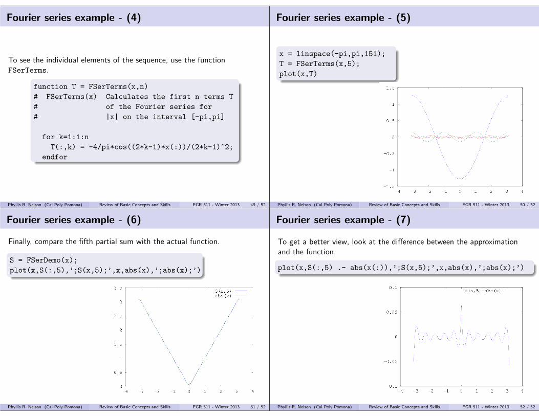
Fourier series example - (4)
To see the individual elements of the sequence, use the functionFSerTerms.
function T = FSerTerms(x,n)# FSerTerms(x) Calculates the first n terms T# of the Fourier series for# |x| on the interval [-pi,pi]
for k=1:1:nT(:,k) = -4/pi*cos((2*k-1)*x(:))/(2*k-1)^2;
endfor
Phyllis R. Nelson (Cal Poly Pomona) Review of Basic Concepts and Skills EGR 511 - Winter 2013 49 / 52
Fourier series example - (5)
x = linspace(-pi,pi,151);T = FSerTerms(x,5);plot(x,T)
Phyllis R. Nelson (Cal Poly Pomona) Review of Basic Concepts and Skills EGR 511 - Winter 2013 50 / 52
Fourier series example - (6)
Finally, compare the fifth partial sum with the actual function.
S = FSerDemo(x);plot(x,S(:,5),’;S(x,5);’,x,abs(x),’;abs(x);’)
Phyllis R. Nelson (Cal Poly Pomona) Review of Basic Concepts and Skills EGR 511 - Winter 2013 51 / 52
Fourier series example - (7)
To get a better view, look at the difference between the approximationand the function.
plot(x,S(:,5) .- abs(x(:)),’;S(x,5);’,x,abs(x),’;abs(x);’)
Phyllis R. Nelson (Cal Poly Pomona) Review of Basic Concepts and Skills EGR 511 - Winter 2013 52 / 52