562 PROCEEDINGS OF THE IEEE, VOL. 69, NO. 5, MAY 1981

Correspondence Processes- m ; Dynamic Scene Analysis

J. K. AGGARWAL, L. S . DAVIS, AND W. N. MARTIN

Invited Paper

Abstmct-One of the fundamental problems in dynamic scene analy- sis is the tracking of objects from frame to frame. A general approach to tracking is to establish correspondences between points, or sets of points, between frames and then group the sets into objects based upon similarity of motion. This paper will focus on processes for establish- ing the correspondence between sets of points in successive frames. A succession of correspondence processes are discussed, based on the factors which contribute to the complexity of the correspondence problem.

I. INTRODUCTION OMPUTATIONAL models for the analysis of time se- quences of images of dynamic scenes are crucial for the solution of many image understanding problems. For

example, in meteorology, the automatic prediction of frontal positions from satellite images of cloud cover requires that the movements of clouds be tracked from image to image [ 1 1. In fact, meteorological applications imparted the initial impetus to research in motion analysis. The spectrum of applications has widened dramatically in the past several years to include biomedicine, tactical and strategic military applications and industrial automation. In addition to this variety of real-world problems, models for motion analysis are of fundamental importance to our understanding of the human visual system. Mammalian visual systems not only contain “software” for motion analysis [2] , but apparently also include “hardware” for the detection of moving objects in the visual field [ 31, [4] .

Perhaps the most prevalent problem in motion analysis is the tracking of objects from frame to frame. Tracking is a prerequisite for computing either the motion of the object or a description of how the object is changing. A general approach to tracking is to establish correspondences between points, or sets of points, in successive frames and then to group those sets into objects based on similarity of motion. Such grouping operations are often based on the assumption that the objects are rigid or that they are articulated (i.e., jointed) but composed of rigid parts. Such assumptions im- pose structural constraints on the relative positions of object points, which in turn impose constraints on the two-dimen- sional pattern of positions projected by those points onto the image plane. For example, Ullman [ 51 and Roach and Aggar- wal [6] use the rigidity assumption to compute the three- dimensional structure of moving objects from multiple views

work was supported by in part funds derived from the National Science Manuscript received July 3, 1980; revised October 23, 1980. This

Foundation under Grant ENG-7904037 and the Air Force OTrke of Scientific Research under Grant AFOSR 77-3190.

Department of Computer Science, The University of Texas, Austin, J . K. Aggarwal is with the Department of Electrical Engineering and

TX 78712. L. S. Davis and W. N. Martin are with the Department of Computer

Science, The University of Texas, Austin, TX 78712.

of the object in motion, while Webb [7] and Rashid [8] dis- cuss how jointed objects may be analyzed. It is important to note that in a great number of applications the objects in mo- tion can be treated as two-dimensional so that grouping opera- tions and accompanying computational models of motion can be specified solely on the basis of changes in image coordinates.

This paper will focus attention on processes for establishing the correspondence between sets of points in successive frames. It should be pointed out that these correspondence processes have applications to other problems in image understanding besides motion analysis-e.g., stereopsis, change detection, etc. We will not consider the subsequent grouping procedures which establish structure and motion from such correspon- dences. Discussions of those problems can be found in [SI, [61.

There are a .number of factors- which contribute towards making the correspondence problem quite difficult; the presence or absence of such factors determines the procedures which can be applied to solve any specific correspondence problem. First, the types of transformations that objects can be subject to from frame to frame must be considered. Can the objects change their orientation in the field of view, or their size? Can their shape change, and if so, is any prior in- formation available which constrains such changes? (This is especially important for tracking clouds, which change shape, sometimes dramatically, from frame to frame.)

Objects may be moving against changing backgrounds, and this tends to complicate the correspondence processes. It is much simpler to track an object which is moving against a clear blue sky than it is to track an object which is moving along the ground from one type of textured region to another. Furthermore, if it is possiblz for the object to move behind other objects, so that it is only partly visible at times (or even completely invisible for some time) then the correspondence processes must be able to establish their matches given only partial information.

We will consider two general approaches towards establish- ing a correspondence between image parts in successive frames. The first is based on constructing “iconic” or picture-like models of a segment of one frame. Such iconic models are sometimes referred to as templates in the picture processing literature. Early psychological theories of visual perception attempted to account for human pattern recognition based on iconic memory models. However, such theories fail to account for recognition of patterns that are highly abstract, or generalized (e.g., the recognition of caricatures, cartoons, etc.). Similarly, computational theories of pattern recognition based on iconic pattern representations are not applicable in all situations. Nevertheless, the computational efficiency of algorithms for matching iconic models against images justifies

0018-9219/81/0500-0562$00.75 0 1981 IEEE

AGGARWAL et al.: DYNAMIC SCENE ANALYSIS 563

their serious consideration before more general modeling tech- niques are adopted.

The second approach employs structural models for seg- ments of the first frame, and then computes homologous representations for segments of the second frame against which it matches those pieces. Such procedures can, in general, tolerate grosser changes in size, shape, etc., than can procedures based on iconic models. They are, however, com- putationally more complex.

11. TRACKING USING ICONIC MODELS In tracking using iconic models, one must first “lock-on,’’ or

detect a subset of the first frame which one suspects contains a moving object, construct an iconic representation of that subset, and then match that iconic representation against the second frame. Suppose that for the frame acquired at t i ,

F1 = f ( x , y , t l ) , x1 G X G X Z , Y 1 GY GY2

is a subimage that contains a moving object. For F1 we define

A x = x 2 - x 1 and A y = y z - y 1 .

Then there are a variety of iconic representations which can be constructed based on F1. These include

1) usingF1 directly; 2) segmenting F 1 into a binary image (i.e., an image com-

posed of 0’s and l’s), where the 1’s indicate object points and the 0’s nonobject points;

3) applying an edge detection operation to F1 resulting in a binary image where the edges, or boundaries, of the objects are labeled 1, and all other points are labeled 0.

The advantage of using F1 directly is that it requires the minimal amount of computation to construct the iconic repre- sentation. However, the exact gray levels in F1 depend not only on the properties of the moving object (e.g., its reflec- tance and shape), but also on the properties of the background against which it is moving. If this background can change dramatically, relative to the object, from frame to frame (e.g., if the background is textured), then it might prove difficult to match F1 based upon this direct representation.

On the other hand, segmenting F 1 into either an object/ background or edge/no-edge representation makes the salient shape characteristics of the moving object explicit in the iconic representation. One must be able, however, to compute such segmentations reliably. In the remainder of this section we will denote by F; the iconic representation of F1. Suppose

F 2 = f ( x , y , t 2 ) , O G x G n , O G y G m ,

is the frame acquired at time t 2 . In order to match F1 against a piece of F z (i.e., a subset of F2 having the same shape and size as F1) one must first compute an iconic representation of that subset which is of the same form as the representation chosen for F 1 . We will let Fi refer to that iconic representation

Next, one must adopt some measure of match between F ; and F;. The measures may be either similarity measures (high values indicate match) or difference measures (low values indicate match). A variety of such measures have been con- sidered including the following.

of Fz.

1) Normalized cross correlation (similarity measure)

where

3) Sum of squared differences (difference measure)

S(X, v) = 2 [ ~ l ( x l + i , y1 +i) - + i, Y + j ) l Z . (3) A x A y

i = O j = O

The normalized cross correlation is closely related to the sum of squared differences since

A x A y

+ F2(x + i , y +jIz i = o j = o

and if F: and 2 x F: were fixed, then S(x , y ) would be minimized when

A x A y Fl(xl + i , y l + j ) Fz(x + i, y +i)

i=o j = o

is maximized. This latter quantity is the unnormalized cross correlation. One must normalize it as above because the unnormalized cross correlation will be high in areas of F2 having high average intensity, whether or not they match F 1 . For C(x , y ) , it is easily shown that 0 < C ( x , y ) < 1, and that C ( x , y ) = 1 if and only if for some constant c [ 9 ]

From the point of view of computational expediency, the difference measures (2) and (3), are preferable to the similarity measure (1) because their cumulative nature (see below) allows them to be incorporated into fast matching algorithms.

The straightforward space-domain algorithm for computing any of the preceding match measures requires A x A y opera- tions per pixel. If A x and A y are large, then this can take a significant amount of computing time on a general-purpose computer. We will discuss two approaches toward reducing this time

1) the use of special-purpose computer architecture;

5 64 PROCEEDINGS OF THE IEEE, VOL. 69, NO. 5, MAY 1981

2) the development of faster algorithms for general purpose computers.

There are at least three distinct types of architectures for image processing which can profitably be distinguished; each is accompanied by its own specific set of advantages, disad- vantages, and theoretical and practical problems.

1) “Focal-plane architectures” which are actually integrated into video sensors behind the focal plane and which are capable of processing data at high-quality television data rates (7.5 MHz).

2) Cellular arrays of simple, bit serial processing elements (PE’s). Cellular arrays are a special class of single-instruction stream multiple-data stream (SIMD) machines having fixed- interconnections.

3) General multiple-instruction stream multiple-data stream (MIMD) machines with many general-purpose processors, memories, and a flexible interconnection network. Such machines can also be operated as SIMD machines.

As one moves4rom architectures of type 1 through type 3, there is a significant decrease in speed. Focal plane archi- tectures can compute a relatively complex computation (e.g., a 5 X 5 convolution) at the rate of 100 ns/pixel, while a cellu- lar array such as CLIP 4 [ 101 and MIMD machines (such as ZMOB [ 111 ) would operate at significantly lower data rates (see Davis [ 121 for more details).

Balancing this decrease in processing efficiency is an in- crease in processing generality. Focal plane architecture is functionally quite rigid; it cannot, e.g., be used to apply iterative algorithms to an image unless the number of itera- tions is known a priori. Even then, it requires duplication of circuitry (e.g., the median of median operation com- puted by TI VLSI architecture [ 131). The cellular arrays are more general, since their PE’s are ordinarily capable of com- puting any Boolean function over a single bit plane of a point and a simple function of its four or eight neighbors. How- ever, for nonlogical operations, the PE’s are very difficult to program due to their “low-level” instruction set. MIMD machines composed of many microprocessors are still more general, since not only are the microprocessors’ machine instructions ordinarily quite powerful, but compilers are available for translating high-level languages (such as Pascal or Fortran) into the machine language of the microprocessors. However, difficult problems in scheduling and sharing need to be solved before MIMD machines become generally available.

For the purposes of object tracking using iconic matching techniques, focal-plane architectures would be most preferable because they can support such computations at close to real- time data rates. As one example of a “focal-plane architec- ture” for convolutions, consider the approach suggested by Texas Instruments (TI) [ 141 based on VLSI technologies.

In general, the correlation of a sequence X = { X i } E o with a sequence of weights W = {Wi}T=o is defined by

n

j = o C(i ) = ~ j ~ [ i + i l . (4)

where [ . ] denotes modulo m . This is essentially the one-dimensional form of the unnor-

malized cross correlation discussed above. It is possible to extend the design discussed the following to normalize C(i) by zTZ0 X [ i + j l , but the principle point of the design is the effi- cient computation of C(i) . Now if we express X, as

1

xn = X n , b 2 b , x n , b E 1} (5 1 b=O

then by substituting (4) into (5) and reordering terms we can obtain

r r n \

Thus C(i ) can be computed using a total of about rn shifts and adds. However, time can be saved by prestoring all values of

j = o

in a 2n by B , + logz ( n ) bit READ-ONLY memory (ROM) where B , is the number of bits required to store the maxi- mum Wi. Now, the computation of C(i) takes r + 1 table look-ups in the memory, and r + 1 shifts and adds. This tech- nique is called the ROM-accumulator (RAC) technique.

An advantage of TI’S VLSI design is that the dynamic range of the convolution weights can be increased with only a small increase in ROM. On the other hand, the VLSI approach is impractical for large convolutions. Even a small, 10 X 10 con- volution would require a ROM which is 2lo0 X (B, + logz n ) bits, which is clearly impossible. If one adopted the blocking schemes suggested in [ 141 (i.e., essentially break the large memory into several smaller memories and then combine the results with additional circuitry), then the architecture might become too slow. Note that one is also faced with the formidable problem of loading the partial product memory (which for image tracking could obviously not be constructed with ROM). This requires both computing all the partial products, and then storing them into memory. Such prob- lems need to be faced before such architectures could be applied to tracking problems. See [ 151 for an alternative architecture based on charge-coupled devices.

An alternative to using special purpose architecture is to design fast algorithms for computing the location of maximum match. Although it is possible to use frequency domain tech- niques, we will restrict our attention to space domain tech- niques because they generalize to wider classes of match functions.

Barnea and Silverman [ 161 introduced a class of fast algo- rithms for image registration which avoided the comparison of every point in FI with every point in F;. In the following, we present a generalization of some of the ideas presented in [ 161 which involves representing the matching problem using state- space representation techniques, and then searching for the best match using an ordered search algorithm. For notational convenience, we will develop the algorithm using only one- dimensional pictures.

Let q(i) , 0 Q i Q m , be a sequence of numbers which repre- sents a one-dimensional image and let p(i) , 0 Q i Q n, n < m represent a one-dimensional object whose position in q we want to detect. We say that the sequence p f {pi}?=o is an initial sequence of a second sequence p t = { ~ i } p = ~ if

a) n Q n’ and b) pi = pi , 0 Q i Q n .

Let M be any cumulative mismatch function for matching a sequence p = against a sequence q = { q i } E o . M is cumulativq iff when p = is an initial subsequence of p t = {P:)?=,, M ( P , q ( j ) ) Q M(p’ , q( j ) ) . Here, M ( P , d j ) ) will be a difference measure that represents the dissimilarity of the sequence p to the subsequence q j , * . . , q j + n -

AGGARWAL e t al.: DYNAMIC SCENE ANALYSIS 5 6 5

As an example, consider the mismatch function A defined as

so that A , is a cumulative mismatch measure.

let ( t , j , M ( p r , q( j ) ) ) where The state-space, then, is defined as follows: A stare is a trip-

1) t indicates how long an initial subsequence of p has been

2) j is a position in q , 3) p f is the initial subsequence of length t of p , and 4) M ( p r , q( j ) ) is the dissimilarity of pr to 4( j ) .

A start state is of the form ( r , j , M ( p r , q ( j ) ) ) , where 1 Q r < n and for each r , 1 Q j < ( m - r ) , while a goal state is one for which r = n. Notice that the start state represents a situa- tion where an initial subsequence of p has been compared to q at position j , while a goal state represents the situation when all of p has been compared to q starting at position j . If S = ( t , j , M ( p f , q( j ) ) ) is a state, then the k-successor of S (denoted o k ( S ) ) is S' where

compared against q starting at position j ,

S' = ( t + k, j , ~ ( p t + ~ , q ( j ) ) )

i.e., S' is obtained by comparing k more points from p against the subsequence of q beginning at j . If S, = O k ( S , - l ) , S,-l = 0 k ( S , - 2 ) , * * e , S2 = O k ( S l ) , then S1, * * * , S, is a path from S1 to S,. The cost of the path is the value of the dissimilarity measure in state S, (which is also the maximum of the dis- similarity measures for the set of states SI, . * * , S,); we will also refer to this cost as the cost of S,. The objective, then, is to find a minimum cost path between a start state and a goal state. This can be accomplished by an ordered search algo- rithm [ 171. The cumulat'lve nature of the mismatch measure assures the admissibility of the algorithm-i.e., it is guaranteed to find a minimum cost path.

The ordered search algorithm is defined as follows. 1) Put al l start states, ( r , j , M(p', ~ ( j ) ) ) , 0 Q j Q m - n, into

a set called OPEN. 2 ) Choose the state from OPEN with minimal dissimilarity

measure and delete it from OPEN. Let S = ( t , j , M ( p r , q( j ) ) ) be this state.

3) If S is a goal state, then the best match of p to q occurs at position j , and the algorithm halts. Otherwise, continue.

4) Compute O k ( S ) and add this new state to OPEN. Go to Step 2.

A slight modification of the above algorithm, employed by Barnea and Silverman [ 161, can lead to dramatic savings in

computation time; however, the algorithm would no longer be admissible. The modification involves not putting into OPEN any state ( t , j , M ( p t , q ( j ) ) ) with M b ' , q ( j ) ) ) T(t) , where T is a threshold function. Barnea and Silverman [ 161 discuss methods for computing a reasonable threshold func- tion from the sequences p and q . We will not adopt this modification in the example below.

As an example of the application of the algorithm, consider Fig. 1. Fig. l(a) contains an image q and an object p . The iterations of the ordered search algorithm are described in Fig. l(b), using k = 1, r = 2 and dissimilarity measure A , the sum of absolute differences. The example proceeds as follows. With r = 2 , the initial subsequence of p of length 2 (i.e., 4 7) is matched against the subsequence of length 2 in q starting at each of the positions 0, 1, * * * , 5. For example, at position 3, the mismatch is 14 - 3 1 + 17 - 2 I = 6. For each partial match a state is entered into the set OPEN. The minimal cost state is

With k = 1, o k ( S l ) is obtained by adding the mismatch of p 2 and q 3 to the cost of S1. This mismatch is 12 - 3 I = 1, so that o k ( S l ) is the state S2 = (3, 1, 2 ) , indicating that the initial subsequence of length 3 of p (i.e., 4 7 2) has been matched to q 1 q 2 q 2 . This state, S 2 , is added to OPEN.

S2 is also the minimal cost state at iteration 2, with O k ( S 2 ) being the state S3 = (4, 1,4). Notice that even though S3 is a final state, the algorithm does not terminate. For a final state to be chosen by the algorithm it must be known to be minimal over the current OPEN set, thus S3 must first be placed in OPEN and its dissimilarity measure compared to the measures of all states. At iteration 3 this comparison yields the minimal cost state S4 = (2, 4, 3). o k ( S 4 ) is the state ( 3 , 4 , 6 ) , but at iteration 4 state S5 = ( 2 , 5 , 4 ) is chosen arbitrarily from the minimal cost subset of OPEN, ((2, 5 ,4) , (2 ,0 ,4) , (4 , 1 ,4)} . We next choose ( 2 , 5 , 4 ) whose successor, (3 , 5, 6), is thenplaced inOPEN. Then, at iteration 5, ( 2 , 0 , 4 ) is taken from OPEN, and its successor, (3, 0, 9), is placed on OPEN. Finally, at iteration 6 , goal state (4, 1,4) is chosen from OPEN and the algorithm halts.

Although the ordered search algorithm will decrease the number of comparisons of points in p with points in q , there are two sources of overhead which might render the strategy more costly than the direct approach.

1) The algorithm must maintain a sorted list of states repre- senting partial matches of p to q.

2) If not enough primary storage is available to simulta- neously maintain all of 4 , then the algorithm may need to page pieces of q in and out when the subsequence of q associated with the newly chosen state of Step 2 is found not to be in the currently available storage. This 1 / 0 overhead can'severely degrade the performance of the algorithm.

The computational cost of matching p against q can also be reduced by employing a subtemplate-template matching strategy [ 181. Here, one matches a piece, p' of p against 4 , and then matches the remainder of p only at those points in q where the match of p' is sufficiently good (e.g., higher than some threshold t if using a similarity measure). If p' has n' points, n' < n, then the total amount of computation per- formed by the subtemplate-template matching algorithm is

S = ( 2 , 1, 1).

w( t ) = mn' + mnP

where P is the probability that the match of p' to q ( j ) has a value greater than t for randomly chosen values of j . Note that unlike the ordered search strategy, the subtemplate-template

566 PROCEEDINGS OF THE IEEE, VOL. 69, NO. 5 , MAY 1981

matching strategy is not guaranteed to find the best match since there is a nonzero probability that the match of p’ to 4 at the position which maximizes the match of p to q will be below the threshold t . Note that this false dismissal rate can be kept arbitrarily close to the flase dismissal rate of matching p to 4 in two ways:

1) lowering the threshold t for matching p f against q ; 2) increasing the size of the subtemplate p ’ .

Lowering the threshold, of course, will increase W ( t ) since for t‘ < t , more points in 4 will match p ’ . If t is made too low, then it is possible for W ( t ) to be greater than mn, which is clearly undesirable. Similarly, increasing the size of p f may also increase W ( t ) . Vanderbrug and Rosenfeld [ 181 discuss choices of n’ and t which minimize W ( t ) while keeping the overall error rate below threshold.

A related strategy to subtemplate-template matching is coarse-fine template matching [ 191. Here, one f i t matches an averaged and sampled version p’ of p against a similarly averaged and sampled version q’ of 4 . Positions in 4’ which are good matches to p ’ are then used to guide the application of p to q. Again, there are tradeoffs between reliability and two factors-the size of p’ relative to p and the threshold used in matching p‘ to 4’.

The coarse-fine matching strategy can be further generalized to matching in a pyramid image representation [ 201, [ 21 1. A pyramid is a stack of regularly reduced resolution versions of an image. Tanimoto and Pavlidis [22], e.g., describe an edge detection procedure which operates in a pyramid.

The applicability of these correlation-based matching pro- cedures is limited by a number of factors. The two most im- portant of these for object tracking are the inability to deal with objects whose orientations in the image plane change from frame to frame and the inability to match given only partial information. The structural techniques discussed in Section I11 are designed to overcome these problems.

111. STRUCTURAL MATCHING TECHNIQUES In this section we shall discuss methods which establish the

correspondence between points of interest at consecutive time instances using structural models or domain constraints to guide the process. The points of interest are assumed to be derived from the images by low-level operators which can detect specified components and determine the locations and descriptive feature values of those components. Each such component, together with its features will be referred to as a

token. For example, a simple 3 X 3 edge operator with local nonmaxima suppression could be used to form a token repre- senting an edge which is considered to be centered at a given pixel with a specific orientation and contrast. The function of the matching process is thus to construct a mapping from the set of tokens of one image to the set of tokens of a second image. Clearly, the methods suitable for establishing this mapping depend on the particular attributes retained with the tokens.

However, intertoken constraints imposed either by structural models or the scene domain are also important. Object models can be derived from two primary sources. General descriptive models of the objects or object types expected to occur in the scene can be provided to the analysis system before processing is initiated. In this case the tokens in each image are matched against the descriptive features contained in the models. For a given token in one image the corresponding token in the preceding image is identified as that token which matched the same model feature as the given token. Models can also be derived from the images as they are processed. In this case general information about object formation is used to group the tokens in an image into structures which are a first esti- mate of the object models and provide constraints useful for establishing the correspondence to the tokens in another image. Such scene domain constraints can also be applied to individual tokens, usually in the form of limits imposed on the area of search for matching tokens.

An early system which employed motion measurements for scene segmentation (Potter [ 231 ) formed tokens referred to as “cross-shaped templates.” The attributes of these tokens were the distances (horizontal and vertical) from a given pixel to the nearest gray level discontinuity. To match a given token of this sort from one image a heuristic search of the second image was performed, starting at the image location of the original token. The search expanded outward from that starting posi- tion and continued until either a similarity measure over the token attributes exceeded a threshold, Le., a match was found, or a preset search limit was reached. The displacement be- tween the locations of matched tokens constituted the motion measurement for the tokens of the first image. The segmen- tation of that image was then performed using the constraint that tokens with the same motion measurements were part of the same object.

Two major problems arose for the system. First, the attri- butes associated with the tokens limited the allowable object motions to be simple translations in the image plane. Second,

AGGARWAL et al.: DYNAMIC SCENE ANALYSIS 561

the system attempted to form a token for every pixel in the image plane, thereby incurring extensive computation in the search phase. By considering the distance from each object boundary point, i.e., the gray level discontinuities used in [23], to some central position, a model of the object to be tracked can be used in conjunction with a matching technique to overcome these problems. The matching technique is a generalization of the Hough transform (Duda and Hart [ 241 ) to arbitrary shapes as encoded in boundary list representations (Ballard [25], Davis and Yam [26]) and will be discussed in the following. We will first describe position invariant match- ing, and then describe generalizations to orientation and scale invariant matching.

Let B = {(Xi, Yi)}?=, be a list of boundary points for the shape to be tracked. B might be the set of edge locations in an image window detected by an “interest operator” at time r l . Let p = (X, Y) be any point (in practice, a central point such as the centroid of B will be computationally convenient to use as p ) . Then the Hough-representation of Busing p , H(B, p ) , is the sequence of vectors {d i }?=, , where dxi = X - Xi and

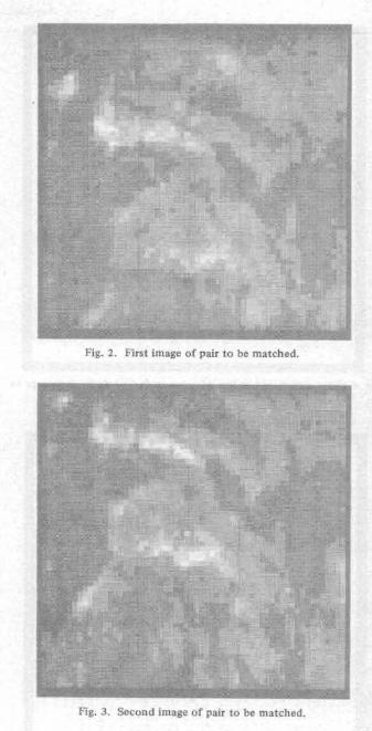
Now, suppose we are given an image f, which contains an dyi = Y - Yi. Fig. 2. First image of pair to be matched.

instance of the shape whose boundary is described by B . Here, f would be the image acquired at time t z . A second array h , which is an array of accumulators that is registered with f, will be used to compute the transform o f f with respect to H(B, p ) . After the transform is computed, points in h with high values will correspond to hypothetical locations of p in f. Of course, once the location of p is known, the instance of B in f can be recovered using H(B, p ) . The array h will be larger than the array o f f , since if the shape is only partly contained in f, the point p might lie outside off.

The transform h is computed by first applying an edge de- tector to f to produce an edge map e of f . Each edge ei in e is a potential element of the set B . Although contrast and orientation information may limit the subset of B to which any ei may correspond, there is, in general, no way to deter- mine the element of B to which any ei corresponds without considering the positions of all the other ei. Therefore, each edge element ei is compared to each vector in H(B, p ) to com- pute a possible location for p , and that location is incre- mented in the transform h . That is, h is computed by the following simple algorithm originally reported in [ 251 :

Algorithm MATCH 1 : For each ei = (Xi, Yi) in e do

For each d i = (dxi , dyi) in H(B, p ) do h(Xi + dxj, Yi + dyi ) : =

h(Xi , + dxi , Yi + d y j ) + 1.

Notice that the result of applying this algorithm is exactly the same as correlating a binary image representation of B with the binary edge map e (this was originally pointed out by Sklansky [27]). The correlation, however, is based on con- sidering all points in h as potential locations for p , and then for each location counting the number of appropriately posi- tioned (according to H(B, p ) ) edges in e. The advantage of the transform algorithm is computational efficiency. If h is an r X s array then to compute h using a standard correlation algorithm requires O(r X s X n) operations-i.e., for each of r X s potential locations for p , we must check the n locations of possible edge points determined by H(B, p ) . Algorithm MATCH 1, on the other hand, requires O( le I X n) operations, where l e I is the number of edges detected in f. Since, in prac-

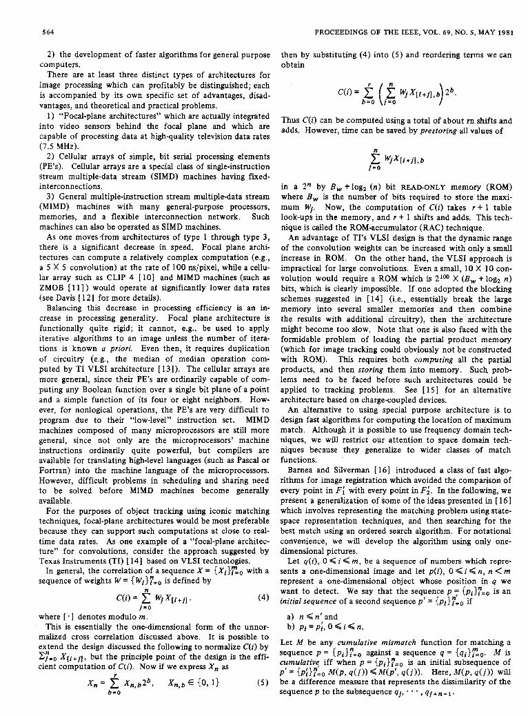
Fig. 3. Second image of pair to be matched.

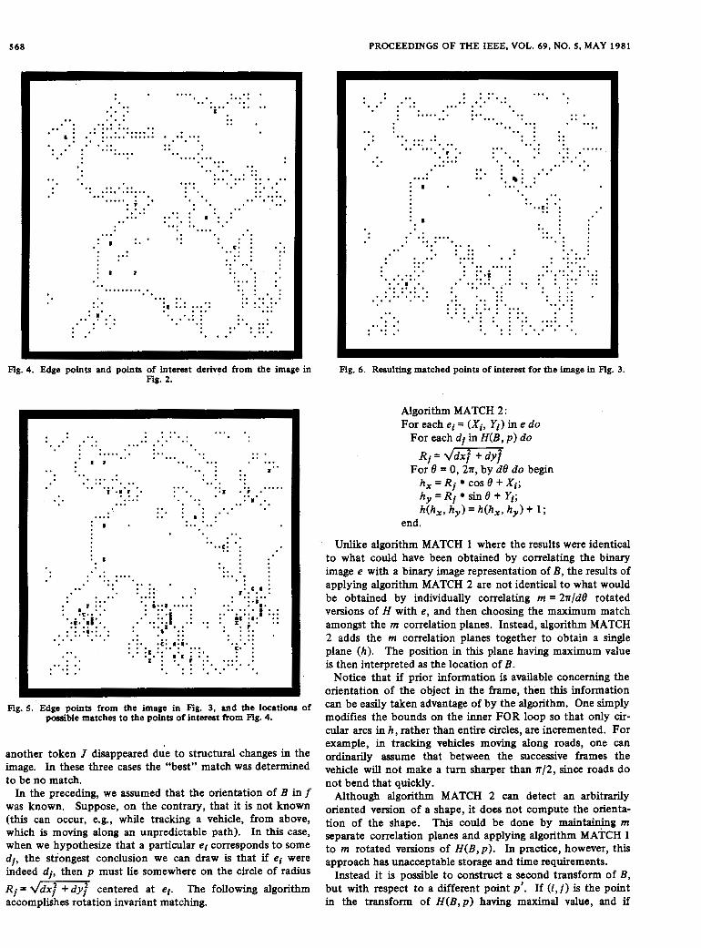
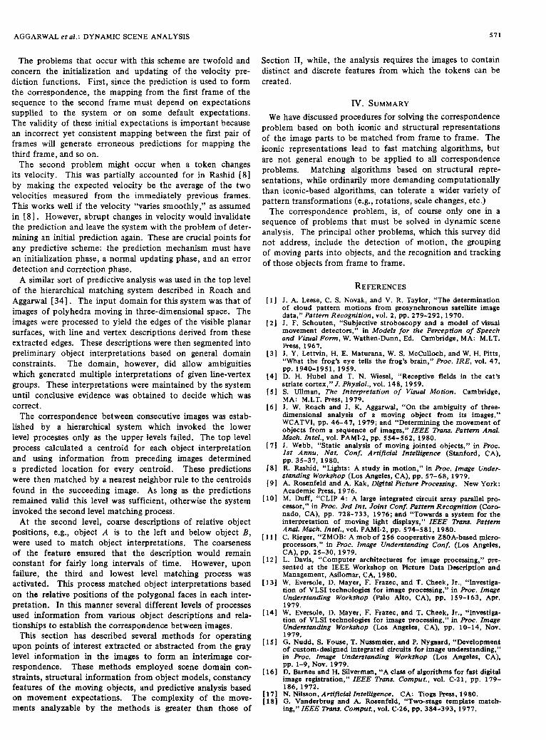
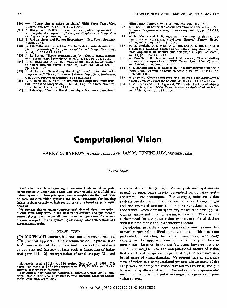
fice, edges account for no more than 5-10 percent of any image, algorithm MATCH 1 will result in speedups of 10 to 20 over conventional correlation procedures. As an example of this process, consider the two aerial photographs contained in Figs. 2 and 3. The objects in these images appear to move toward the top of the image. Fig. 4 shows the edge points found in Fig. 2, along with points of interest (marked by letters) derived by grouping edge points into sets, one set per point of interest. A Hough-representation is formed for the set of edge points associated with each point of interest using the location indicated by the letter as the central point. There are ten points of interest, i.e., tokens, in Fig. 4. For each of these tokens a Hough transformation relative to the edge points found in the second image is formed. Fig. 5 shows the edge points for the second image in addition to the positions of the five highest peaks in each transform. Intertoken con- straints were then employed to determine the “best” matches. Note that two tokens, G and I , moved off the image and

568 PROCEEDINGS OF THE IEEE, VOL. 69, NO. 5, MAY 1981

I

ge il

* . . . . . .. . .

. . . .

. . . . . . . . *. . . . . . . . . . . . . . . . . . . . . . . . . . . . . . . . . . . . . . . . .. .... .. . . . . . . . . . .. . . . . . . . .. . . . . ...... . . . . .. . .

a : - . . . . . . . . . . . . . . . .

. . . . . . . . . . ............ . . ... .... ..... . . . . . . . . . .. .. . . . ....... . . . . . .. .. . . . . . . . . . . . . . . . . . . . . . . . . . . . . 1 : ..... . . . . . *.

. . . . . . . . . . . . . . . . . . ... . . . . . . . . . * _ ! _. . . . . . . . . . . . . .. . . . . . * .. . . . . . . . . . . . . . . . . . . . . . ...... . . . . . .. ..

. . . . . . . * * e : : . . .. . . . . . . . . . . . . . . . . . . . . . . . . . . . . . . . . . . . . . . . . . . . . . . . . . . . . . ... .. * . . . . . . . . . . . . . . . . .

. . . .... . . . . . . . . . . . . . . . . . . ... . . . . . . .... .. .* : : . . . ..... . . . . . . ........... ... , . .....

: i :* . . . ... .. ... . . . , .. . . . . . . : I I .. ..........

. , . . . . . . . . . .. ... .. . . .... . . . . . . I . . . . . . . . . . . . . . . . . . .

.... . . . . . . . . . . . ..

. . .. ... . . . .

.. * . . . . . . . . . . . . . . . . . . . . . .. .. * .. . . ...... . . . . ........ . . . . . . . . . . . . . . . . . . . . . . . . . . . * ::! : . . . . . . . . . . . . . . . . . . . . . . . . . . . . . . .. . . . . . . . . . . . . . . . . . . I . . . . . . . . . . . . . . . . . . . . . . . . . . . . . . . . . . . . .

..... . . . . . . . . . .. . . :E - * . :*:: . . . . .: ! :. . . . . . . . . . . . . . . . . . . . . . . . . . . . . . . . . . . . . . . . . . . . . . . . . . . . . . . . . . . . . . . . . . . . . .

Fig. 4. Edge points and points of interest derived from the ima Ftg. 2.

Fig. 6. Resulting matched points of interest for the image in Fig. 3. n

Algorithm MATCH 2 : For each ei = (Xi, Yi) in e do

For each di in H(B, p ) do

For 6 = 0 , 2 n , by dB do begin Ri = 4- hx = Ri * COS 6 + X i ; h y = R i * S i n 6 + Y i ; W X , hy) = Nh, , h y ) + 1 ;

end.

Unlike algorithm MATCH 1 where the results were identical to what could have been obtained by correlating the binary image e with a binary image representation of B , the results of applying algorithm MATCH 2 are not identical to what would be obtained by individually correlating m = 2n/d6 rotated versions of H with e, and then choosing the maximum match amongst the m correlation planes. Instead, algorithm MATCH 2 adds the rn correlation planes together to obtain a single plane ( h ) . The position in this plane having maximum value is then interpreted as the location of B .

Notice that if prior information is available concerning the orientation of the object in the frame, then this information can be easily taken advantage of by the algorithm. One simply modifies the bounds on the inner FOR loop so that only cir- cular arcs in h , rather than entire circles, are incremented. For example, in tracking vehicles moving along roads, one can ordinarily assume that between the successive frames the vehicle will not make a turn sharper than n / 2 , since roads do not bend that quickly.

Although algorithm MATCH 2 can detect an arbitrarily oriented version of a shape, it does not compute the orienta- tion of the shape. This could be done by m a i n w g m separate correlation planes and applying algorithm MATCH 1 to m rotated versions of H(B, p ) . In practice, however, this approach has unacceptable storage and time requirements.

Instead it is possible to construct a second transform of B , but with respect to a different point p’ . If (i, j ) is the point in the transform of H ( B , p ) having maximal value, and if

. . ..

. . . ... . . ... .. . . . . . . . .. . . . . . . . . . . - B I .. . . . . . . . . . *. . .. . . . . I . . . . . . . . . . . . ... . . . . . . . . . . . .I . r . . . . . . . . . . . . .: :.

.. ...... . . . . . . . . . . . . . I .! ! *. ....

9 . .

. . . . . . . . . . . . . . . . . . . . . . . . . . . . .... . 1 *

* I

. . . . . . . . . . . . . . . . . *. . . . . . . . . . . . ,..e.‘ :

. . . . . . . . . . .... . . . . . . . . . i.1 . . . . . II :.: .. I. . . . . . : :; if : .. ..

. . . . . . . . . . . . . F’ : . . . . . . . . . . .

. . . ‘..I ..... . . . :xi . i .. : **IE *.: * . . . . . . . . . . . . . . . . :c:..:,-. .. . . .s . . . . . . . . . . : ! *E i *::

.. . . . . . . . . . . .

. . . . . . . . . . . . . .

Fig. 5. Edge points from the image in Fig. 3, and the locations of possible matches to the points of interest from Fig. 4.

another token J disappeared due to structural changes in the image. In these three cases the “best” match was determined to be no match.

In the preceding, we assumed that the orientation of B in f was known. Suppose, on the contrary, that it is not known (this can occur, e.g., while tracking a vehicle, from above, which is moving along an unpredictable path). In this case, when we hypothesize that a particular el corresponds to some dj , the strongest conclusion we can draw is that if el were indeed di , then p must lie somewhere on the circle of radius Ri = centered at el. The following algorithm accomplishes rotation invariant matching.

AGGARWAL et al.: DYNAMIC SCENE ANALYSIS 569

(i’, j ’ ) is the point in the transform of H ( B , p ’ ) having max- imal value (notice that these values must, in principle, be identical), then the direction from ( i , j ) to ( i ‘ , j ‘ ) gives the direction from p to p’ in f. Points p and p’ should be cho- sen to be sufficiently far apart so that small errors in the locations of the maxima in the transforms h of H ( B , p ) and h’ of H ( B , p ’ ) do not lead to large errors in the computed orientation of B .

Notice that the algorithms can also be modified in a straight- forward way to deal with a limited range of scale informa- tion. Suppose, e.g., it is known that the object in the image is S times the size of the model, with S E [S,, Sz] (note SI < S2 and 0 <SI). Then in algorithm MATCH 1 rather than just incrementing a single point at distance d =- from an edge point, one marks a l l points in direction tan-’ (dy/!,) and with distances d’ E [Sld, Szd] . For rotation invanant matching, rather than incrementing a circle (or circular arcs if constraints on the orientation are available) one increments a ring of inner radius Sld and outer radius S2d (or the inter- section of the ring with wedges). Again, different correlation planes can be maintained for different values of the scale, but this increases the storage and computational requirements of the matching algorithms. Note that this idea was employed by Davis [28 ] to detect circles of various sizes using Hough- transform techniques.

Boundary descriptions of objects were also employed by the system discussed in Martin and Aggamal 1291. This sys- tem extracted simple closed curves representing figures with curvilinear boundaries from each image in a time ordered sequence. In this case the input was restricted so that the figures independently moved in planes parallel to the image plane. The figures were planar with opaque homogeneous shading. This meant that when the figures moved so as to occlude one another the boundaries merged into apparently single figures. The main task of the system was thus to derive descriptions of the actual figure boundaries which were con- stituents of the apparent figures in the images.

The fact that a given figure in the image might be composed of boundary points from several actual figures precluded the matching of the entire boundary between two images. Instead the boundaries were broken into sets of tokens with each token representing a boundary section which approximated a straight line or a circular arc. The token attributes were the length and curvature of the represented arc. The matching process began by finding pairs of highly similar tokens, re- ferred to as “seeds.” The remainder of the matching process made use of the ordering of the tokens on the figure bound- aries to constrain the segment “growing” algorithm that was applied to the already matched “seeds.”

This process was able to detect extended boundary segments having the same shape in consecutive images. Since the actual figures were assumed to be rigid, a pair of matched segments could be interpreted as being two views of a portion of an actual object boundary. Thus the boundary shapes were used to form the correspondence which in turn provided motion measurements for each matched segment. The final grouping into actual objects was based on the constraint that segments exhibiting similar motions were sections of a single rigid object.

This latter constraint is quite important and is the basis of the object interpretation in most current motion analysis systems. However, for the correspondence processes in the systems discussed so far in this section, the matching has been

based on token attributes not related to motion. In the re- mainder of this section we will illustrate how the motion or the expected motion of ‘the scene components can be used in forming the correspondence.

Endlich et al. [ 301 did not incorporate an explicit movement expectation but did assume that most of the tokens within arbitrarily chosen subimages exhibited similar velocities. Under this assumption their system formed a Correspondence which specified a consistent velocity for the largest number of tokens in a subimage. The tokens were referred to as “brightness centers” and had an intensity attribute as well as an image location. The procedure used by the system was to iteratively refine the estimate of the representative velocity and to use the estimated velocity to constrain the possible matches for each token. The process was iterated until each token had no more than one possible match.

The velocities determined for each subimage were then merged together to yield a velocity map which represented the cloud motions in the satellite images processed by this system. For more general image sequences, however, the arbitrary partitioning of the image into subimages could be a severe problem because the presence of two or more inde- pendently moving scene components in a given subimage would invalidate the assumption of a representative velocity for that subimage. In most cases it will be impossible to know a priori how to partition the image so that each sub- image contains only one scene component. One might, however, make use of the localized motion consistency con- straint in a network of competing hypotheses, much like the consistent labeling procedures of Rosenfeld et al. [ 3 1 ] .

Barnard and Thompson [321 accomplished this by locating the prominent (i.e., most likely matchable) features in each of a pair of images with an “interest operator.” Associated with the operator was a similarity measure which was used both to initialize the “probabilities” for the hypothesized matches at the tokens and to update those “probabilities” at each iteration of the refining process. The network upon which this refining process operated was created from the tokens in the f i t of the pair of images by establishing a node for each token and connections between all nodes whose tokens were within a preset distance of each other. At each node a “label” set was formed containing an element for each possible match of the associated token. The labels were ordered pairs of -the disparity, in the x and y directions of the image plane, between the location of the token of the node and the location of each token within a given radius of that position in the second image of the pair.

In addition to the possible match labels, there was included a special label specifying that no match could be found for the given token. The inclusion of this special label is indicative of an important concept for motion analysis systems: the track- ing procedures must be robust enough to continue functioning properly when some of the features of interest, i.e., the tokens currently being tracked, are no longer detectable in the image. A particular feature may not appear in a given image of the sequence for several reasons: the feature might become oc- cluded by scene components of the foreground; the image characteristics might for some reason, e.g., illumination changes, not remain within the tolerances of the interest operator; or the feature may move beyond the view of the imaging device.

The motion consistency constraint of Barnard and Thompson 1321 was propagated throughout the network by increasing

570 PROCEEDINGS OF THE IEEE, VOL. 69, NO. 5, MAY 1981

the probability assigned to a given label at a specified node by an amount proportional to the sum of the probabilities of the similar labels at connected nodes. This label r e f i i g process could be iterated until the network stabilized or until every node had a clearly defined “most likely” label. However, i n , practice it was iterated ten times, leaving a few ambiguous labelings.

A network of a different sort was proposed by Ullman [ 51. Here, a node was associated with each token in the pair of consecutive frames. For each token in one frame the set of possible matches in the other frame was determined and connections were established between the node for the given token and the nodes for the tokens in the matching set. This network was used to calculate the correspondence which minimized a mapping cost function. The calculation was to be performed by simple processors, one attached to every node and connection in the network. Each node processor communicated with the processors attached to the connections incident on that node, while each connection processor com- municated with the Processors at the two nodes which ter- minated the connection. Thus the processors could be par- titioned into three disjoint sets: one set associated with the tokens of the first frame; another set related to the tokens in the second frame; and the fiial set representing possible matches between two tokens, one from each frame. All processors computed only simple functions of values

stored at the neighboring processors and used those func- tions to update their own values. This updating procedure was iterated until the values in the network stabilized, at which time the connection processors had values of either 1 or 0, only. The resulting correspondence was then specified by the set of connection processors that had a value of 1, i.e., a given token of the first frame was mapped to a token of the second frame if the nodes for those tokens were con- nected in the network and the processor attached to that connection had a value of 1. Thus the specified correspon- dence was the mapping which yielded the minimal cost.

The cost function proposed was directly related to the probability distribution of the velocity of the tokens as measured in the images. Minimizing this cost function was shown by Ullman [ 51 to be optimal under the assumption that the movement of each token was independent of the movements of the other tokens. It was also argued that one-to-one mappings should be preferred and then shown that a simple modification to the cost function would effect this preference.

As the time between frames increased and the velocities of the tokens decreased, the mapping also tended to IIlinimize the total distance moved by all tokens in the scene. This was the case in which the nearest neighbor match of the tokens tended to be a one-to-one mapping. At higher velocities nearest neighbor matching would result in numerous “splits” and “fusions,” i.e., one-to-many and many-to-one mappings, while the “optimal” cost minimizing mapping would retain its preference for one-to-one mappings. In this way, although the nearest neighbor match might not be the desired corre- spondence, it could be used as the initial estimate for the minimizing process which derives the “optimal” mapping. Thus the network would be constructed by connecting the node of a given token in one frame to the N nodes associated with the N nearest tokens from the other frame. It should be noted that there is no mechanism for adding connections to the network once the minimization process has begun,

so the -initial set of possible matches would have to contain the “correct” one.

There were two major problems with the overall scheme proposed in Ullman [SI for forming the correspondence between frames. The first was similar to the problem of subimage selection of Endlich et al. [30], in that the cost function used a single distribution for the velocities. This was justified by the independence of movement assumption. Clearly, the validity of this assumption would be in doubt if several tokens were established for each object in the scene. In that case the motions of the tokens associated with a par- ticular object would be interdependent and directly related to the overall movement of the object. The second problem was the requirement that the correspondence be specified by a “cover,” i.e., every token in both frames was matched. Note that for the examples studied in Ullman [5] this was not a problem because the images were of dot patterns in which occlusion was rare. However, for general scenes the features that give rise to tokens will frequently disappear and appear necessitating the no-match possibility, as discussed earlier in this section. A solution to this problem might be to introduce into the original network two special nodes for which the connection would mean “no match.” Initially all the nodes for a given frame would be connected to one of the special nodes and all the nodes for the other frame would be connected to the remaining special node. The difficulty here would be determining the cost associated with the no match connection as it relates to the velocity distribution and the one-to-one mapping preference.

The expected velocity of a token was also used in the correspondence forming process of the system described in Rashid [81. Again, the input was a sequence of images of dot patterns with a token created for each dot. In this case, however, each token retained its own expected velocity parameter. The expectations were used to determine the predicted locations for the tokens from one frame. Those computed locations were then matched against the tokens in the next frame. The desired Correspondence was the one-to-one mapping from the set of predicted locations to the set of tokens for the new frame which minimized the sum of all the distances between the predicted locations and their matched tokens.

The minimization was not computed by a network of simple processors. Instead, a Voronoi construction (Shamos [33]) was used to provide an efficient implementation. For a set of N locations a Voronoi construction tessillates the plane into N polygons (some possibly infinite in size). Each polygon is associated with exactly one of the locations in the set and bounds the area containing all the points for which the associated location is the closest element of the set. Thus to determine the closest location to a point, one need only ask which polygon of the Voronoi construction contains that point. In Rashid [8] a Voronoi construction was performed for the set of predicted locations from a given frame, then each token of the new frame was matched to the closest pre- dicted location by finding which polygon included the token. If more than one token was within a single polygon then the token nearest to the associated predicted location was chosen as the match for that location. The matched location was deleted from the set and a new Voronoi construction was computed. The efficiency lies in the fact that given a Voronoi construction for N points, computing a new construction using N-1 of those points is linear in the number of points.

AGGARWAL et al . : DYNAMIC SCENE ANALYSIS

The problems that occur with this scheme are twofold and concern the initialization and updating of the velocity pre- diction functions. First, since the prediction is used to form the correspondence, the mapping from the first frame of the sequence to the second frame must depend on expectations supplied to the system or on some default expectations. The validity of these initial expectations is important because an incorrect yet consistent mapping between the fmt pair of frames will generate erroneous predictions for mapping the third frame, and so on.

The second problem might occur when a token changes its velocity. This was partially accounted for in Rashid [8] by making the expected velocity be the average of the two velocities measured from the immediately previous frames. This works well if the velocity “varies smoothly,” as assumed in [8]. However, abrupt changes in velocity would invalidate the prediction and leave the system with the problem of deter- mining an initial prediction again. These are crucial points for any predictive scheme: the prediction mechanism must have an initialization phase, a normal updating phase, and an error detection and correction phase.

A similar sort of predictive analysis was used in the top level of the hierarchical matching system described in Roach and Aggarwal [34]. The input domain for this system was that of images of polyhedra moving in three-dimensional space. The images were processed to yield the edges of the visible planar surfaces, with line and vertex descriptions derived from these extracted edges. These descriptions were then segmented into preliminary object interpretations based on general domain constraints. The domain, however, did allow ambiguities which generated multiple interpretations of given line-vertex groups. These interpretations were maintained by the system until conclusive evidence was obtained to decide which was correct.

The correspondence between consecutive images was estab- lished by a hierarchical system which invoked the lower level processes only as the upper levels failed. The top level process calculated a centroid for each object interpretation and using information from preceding images determined a predicted location for every centroid. These predictions were then matched by a nearest neighbor rule to the centroids found in the succeeding image. As long as the predictions remained valid this level was sufficient, otherwise the system invoked the second level matching process.

At the second level, coarse descriptions of relative object positions, e.g., object A is to the left and below object B , were used to match object interpretations. The coarseness of the feature ensured that the description would remain constant for fairly long intervals of time. However, upon failure, the third and lowest level matching process was activated. This process matched object interpretations based on the relative positions of the polygonal faces in each inter- pretation. In this manner several different levels of processes used information from various object descriptions and rela- tionships to establish the correspondence between images.

This section has described several methods for operating upon points of interest extracted or abstracted from the gray level information in the images to form an interimage cor- respondence. These methods employed scene domain con- straints, structural information from object models, constancy features of the moving objects, and predictive analysis based on movement expectations. The complexity of the move- ments analyzable by the methods is greater than those of

571

Section 11, while, the analysis requires the images to contain distinct and discrete features from which the tokens can be created.

IV. SUMMARY We have discussed procedures for solving the correspondence

problem based on both iconic and structural representations of the image parts to be matched from frame to frame. The iconic representations lead to fast matching algorithms, but are not general enough to be applied to all correspondence problems. Matching algorithms based on structural repre- sentations, while ordinarily more demanding computationally than iconic-based algorithms, can tolerate a wider variety of pattern transformations (e.g., rotations, scale changes, etc.)

The correspondence problem, is, of course only one in a sequence of problems that must be solved in dynamic scene analysis. The principal other problems, which this survey did not address, include the detection of motion, the grouping of moving parts into objects, and the recognition and tracking of those objects from frame to frame.

REFERENCES

of cloud pattern motions from geosynchronous satellite image J. A. Leese, C. S. Novak, and V. R. Taylor, “The determination

data,” Pattern Recognition, vol. 2, pp. 279-292, 1970. J . F. Schouten, “Subjective stroboscopy and a model of visual

and Visual Form, W. Wathen-Dunn, Ed. Cambridge, MA: M.I.T. movement detectors,” in Models for the Perception of Speech

J. Y. Lettvin, H. E. Maturana, W. S. McCulloch, and W. H. Pitts, Press, 1967.

“What the frog’s eye tells the frog’s brain,” Proc. IRE, vol. 47,

D. H. Hubel and T. N. Wlesel, “Receptive fields in the cat’s striate cortex,”J. Physiol., vol. 148, 1959. S. Ullman, The Interpretation o f Visual Motion. Cambridge, MA: M.I.T. Press, 1979. J . W. Roach and J . K. Agganval, “On the ambiguity of three- dimensional analysis of a moving object from its images,” WCATVI, pp. 46-47, 1979; and “Determining the movement of objects from a sequence of images,” ZEEE Trans. Pattern Anal. Mach. Intel., vol. PAMI-2, pp. 554-562, 1980. J. Webb, “Static analysis of moving jointed objects,” in Proc. 1st Annu. Nat. Con5 Artificial Intelligence (Stanford, CA),

R. Rashid, “Lights: A study in motion,” in Proc. Image Under- standing Workshop (Los Angeles, CA), pp. 57-68, 1979.

Academic Press, 1976. A. Rosenfeld and A. Kak, Digital Picture Processing. New York:

M. Duff, “CLIP 4: A large integrated circuit array parallel pro-

pp. 1940-1951, 1959.

PP. 35-37, 1980.

I

cessor,” in Proc. 3rd Znt. Joint Con$ Puttern Rec&-ition (Coro- nado, CA), pp. 728-733, 1976; and “Towards a system for the interpretation of moving light displays,” IEEE Trans. Pattern Anal. Mach. Intel., vol. PAMI-2, pp. 574-581, 1980.

1 1 1 C. Rieger, “ZMOB: A mob of 256 cooperative ZSOA-based micro- processors,” in Proc. Image Understanding Conf. (Los Angeles,

121 L. Davis, “Computer architectures for image processing,” pre- sented at the IEEE Workshop on Picture Data Description and Management, Asilomar, CA, 1980.

131 W. Eversole, D. Mayer, F. Frazec, and T. Cheek, Jr., “Investiga- tion of VLSI technologies for image processing,” in R o c . Image Understunding Workshop (Palo Alto, CA), pp. 159-163, Apr. 1979.

141 W. Eversole, D. Mayer, F. Frazec, and T. Cheek, Jr., “Investiga- tion of VLSI technologies for image processing,” in Proc. Image Understanding Workshop (Los Angeles, CA), pp. 10-14, Nov. 1979.

CA), PP. 25-30, 1979.

[ 151 G. Nudd, S. Fouse, T. Nussmeier, and P. Nygaard, “Development of custom-designed integrated circuits for image understanding,” in R o c . Image Understanding Workshop (Los Angeles, CA),

[ 161 D. Barnea and H. Silverman, “A class of algorithms for fast digital image registration,” ZEEE Trans. Comput., vol. C-21, pp. 179-

-. . ..

PP. 1-9, NOV. 1979.

186, 1972. [ 171 N. Nilsson, Artificial Intelligence. CA: Tioga Press, 1980. [ 181 G. Vanderbrug and A. Rosenfeld, “Two-stage template match-

ing,”ZEEE Trans. Cornput., vol. C-26, pp. 384-393, 1977.

572 PROCEEDINGS OF THE IEEE, VOL. 69, NO. 5 , MAY 1981

- Cybern., vol. SMC-7, pp. 104-107, 1977,

, “Coarse-fine template matching,’’ IEEE Trans. Syst., Man,

A. Klinger and C. Dyer, “Experiments in picture representation with regular decomposition,’’ Comput. Graphics and Image Pro- cessing, vol. 5 , pp. 68-105, 1976. T. Pavlidis, Structural Pattern Recognition. New York: Springer- Verlag, 1978. S. Tanimoto and T. Pavlidis, “A hierarchical data structure for picture processing,” Comput. Graphics and Image Processing,

with a cross-shaped template,” in 4IJCAI, pp. 303-308, 1975. J. L. Potter, “Scene segmentation by velocity measurements

R. 0. Duda and P. E. Hart, “Use of the Hough transformation to detect lines and curves in pictures,” Commun. ACM, vol. 19,

trary shapes,” TR-55, Computer Sciences Dep., Univ. Rochester, D. H. Ballard, “Generalibng the Hough transform to detect arbi-

Oct. 1979, Pattern Recognition, t o be published.

tion for shape recognition,” TR-134, Dep. Computer Sciences, L. S. Davis and S. Yam, “A generalized Hough-like transforma-

J. Sklansky, “On the Hough technique for curve detection,” Univ. Texas, Austin, Feb. 1980.

VOl. 4, pp. 104-119, 1975.

PP. 73-83,1976.

281 L. Davis, “Computing the spatial structure of cellular textures,” IEEE Trans. Comput., vol. C-27, pp. 923-926, July 1978.

Comput. Graphics and Image Processing, vol. 9, pp. 111-122, 1979.

291 W. N. Martin and J. K. Agganval, “Computer analysis of dy- namic scenes containing curvilinear figures,” Pattern Recog

301 R. M. Endlich, D. E. Wolf, D. J. Hall, and k E. Brain, “Use of nition,vol. 11, pp. 169-178, 1979.

a pattern recognition technique for determining cloud motions from sequences of satellite photographs,” J. Appl. Metereol.,

31 ] A. Rosenfeld, R. Hummel, and S. W. Zucker, “Scene labelling by relaxation operations,” IEEE Trans. Syst., Man, Cybern.,

V O ~ . 10, PP. 105-117, 1971.

VOI. SMC-6, PP. 420-433, 1976. [ 321 S. T. Barnard and W. B. Thompson, “Disparity analysis of images,”

IEEE Trans. Pattern Analysis Machine Intel., vol. PAMI-2, pp.

[ 331 M. Shamos, “Closest-point problems,” in Proc. 16th Annu. Symp. Foundationsof ComputerScience (ACM), pp. 151-162, 1975.

[ 3 4 ] J. W. Roach and J. K. Aggarwal, “Computer tracking of objects moving in space,” IEEE Trans. Pattern Analysis Machine Intel.,

333-340, 1980.

VOI. PAMI-1, PP. 127-134, 1979.

Invited Paper

Absrtract-Research is beginning to uncover fundamental computa- tional principles underlying vision that apply e q d y to artificial and natural systems. These principles provide insights into the limitations of euly machine vision systems and lay a foundation for building future systems capable of high performance in a broad range of visual domains.

We present this emerging computational view of visual perception, discuss some early work in the field in its context, and put forward current thoughts on the overall organization and operation of a general- purpose computer vision system, synthesizing recent theoretical and experimental results.

I . INTRODUCTION s IGNIFICANT progress has been made in recent years on practical applications of machine vision. Systems have been developed that achieve useful levels of performance

on complex real imagery in tasks such as inspection of indus- trial parts [ 11, [ 21, interpretation of aerial imagery [ 3 ] , and

Manuscript received July 3, 1980; revised November 13, 1980. This paper was begun at SRI with support from NSF, DARPA and NASA, and was completed at Fairchild.

The authors were with the Artificial Intelligence Center. SRI Interna- tional, Menlo Park, CA. Thev are now with Fairchild Research Labora- tories, Palo Alto, CA 94304.

analysis of chest X-rays [4]. Virtually all such systems are special purpose, being heavily dependent on domain-specific constraints and techniques. For example, industrial vision systems usually require high contrast to obtain binary images and use overhead cameras t o minimize variations in object appearance. Such domain specificity makes each new applica- tion expensive and time consuming to develop. There is thus a clear need for computer vision systems capable of dealing with less predictable and less structured scenes.

Developing general-purpose computer vision systems has proved surprisingly difficult and complex. This has been particularly frustrating for vision researchers, who daily experience the apparent ease and spontaneity of human perception. Research in the last few years, however, Has pro- vided new insights into the computational nature of vision that could lead to systems capable of high performance in a broad range of visual domains. We present here an emerging view of vision as a computational process, discuss some of the early work in computer vision that led to this view, and put forward a synthesis of recent theoretical and experimental results in the form of a putative design for a general-purpose vision system.

0018-9219/81/0S00-0S72$00.75 0 1981 IEEE