1

4.2 EVALUATION OF HPAC-URBAN AND JEM WITH U2000, JU2003, MSG05, AND MID05 TRACER OBSERVATIONS

Steven Hanna*

1, Joseph Chang

2, and Ian Sykes

3

1Hanna Consultants, Kennebunkport, ME;

2Consultant, Fairfax, VA;

3Sage-Management, Princeton, NJ

ABSTRACT An overview is given of our experience over the past few years in evaluating HPAC-Urban and JEM with tracer data from the major U.S. urban field experiments over the past ten years in Salt Lake City (Urban 2000 or U2000), Oklahoma City (Joint Urban 2003 or JU2003), and Manhattan (Madison Square Garden 2005 or MSG05 and Midtown 2005 or MID05). HPAC-Urban includes SCIPUFF with the Urban Canopy (UC), Urban Dispersion Model (UDM), and MicroSwift-Spray (MSS) urban module options; and JEM includes only the UC and UDM options. In each set of evaluations, a few likely options are tested for meteorological inputs (e.g., closest NWS airport site, representative downtown building rooftop, upwind vertical profile from remote sounder, and NWP outputs). The paper summarizes the results of the evaluations, including use of model acceptance criteria in the JEM evaluations. In general we find that there is not a single urban model option or a single type of meteorological input that provides clear improvements over any other. For maximum concentrations on downwind distance arcs, most of the time the relative mean bias has a magnitude less than 0.6 and the relative root mean square error is less than about six. 1. OBJECTIVES AND BACKGROUND This paper gives an overview of evaluations of the Hazard Prediction Assessment Capability (HPAC) - Urban and the Joint Effects Model (JEM) transport and dispersion models with tracer data obtained from four urban field experiments: Urban 2000 (U2000) in Salt Lake City, Joint Urban 2003 (JU2003) in Oklahoma City, and Madison Square Garden 2005 (MSG05) and Midtown 2005 (MID05) in Manhattan. HPAC-Urban has been under development for about ten years and various updates have been released in official versions with labels such as HPAC 4.0 and HPAC 5.0. JEM is intended to incorporate aspects of HPAC and other DoD models and be eventually used by all DoD agencies for atmospheric hazard assessments. JEM has also gone through several release versions. ______________________________________ Corresponding author address: Steven R. Hanna, 7 Crescent Ave., Kennebunkport, ME 04046-7235, hannaconsult@roadrunner.com

The authors have been evaluating these various versions with the field experiment observations for most of the past decade. The results for HPAC-Urban given below use an early version for U2000, use a combination of versions (including 5.0) for JU2003, and use the 2008 HPAC 5.0 version for MSG05 and MID05. The results for JEM use the same early 2010 version for all four urban data sets. Although JEM incorporates HPAC-urban, because of the timing of the various version releases, the results below are likely to show some differences. 2. HPAC URBAN OPTIONS TESTED The components of HPAC/SCIPUFF (Second-Order Closure Integrated Puff) are described by Sykes et al. (2007). Our more recent (2009 and later) evaluations with JU2003, MSG05, and MID05 use Version 5.0 SP1 (DTRA, 2008). The results of the evaluations of HPAC-Urban are described by Chang et al. (2005) for U2000, by Hanna et al. (2008) and Hanna et al. (2009a and b) for JU2003, by Hanna et al. (2009a, b and c) for MSG05, and by Hanna et al. (2009a) for MID05. The evaluations with HPAC 5.0 SP1 use the following HPAC/SCIPUFF urban options:

UC - Urban Canopy (a parameterization of the urban wind and turbulence profiles in SCIPUFF) UDM - Urban Dispersion Model (developed by the Defence Science and Technology Laboratory (DSTL) in England. MSS - MicroSWIFT/SPRAY (a new addition in version 5.0 SP1)

Prior to HPAC 5.0, MSS was not an option and therefore was not tested in the references dated 2008 and earlier. The current runs use up to four alternate sets of meteorological data inputs:

Single (SNG) – Observed winds from a rooftop anemometer on a tall building in the central business district. For JU2003, another related option (AVG) was the average wind speed and direction from all anemometers in the urban area (Hanna et al., 2007) Basic Default (BDF) – National Weather Service (NWS) default based on routine data from a nearby airport data

2

Upwind (UPW) – Single observational wind profile from an upwind site. MEDOC – Mesoscale Meteorological Model – Version 5 (MM5) MEDOC outputs using special 4 km resolution runs by the National Center for Atmospheric Research (NCAR). MEDOC is a special format used just for inputs to HPAC.

Note that SWIFT (or MicroSWIFT for the case of MSS) is always triggered in HPAC for all meteorological input options except for MEDOC, where no additional diagnostic analysis of winds is performed. 3. JEM OPTIONS TESTED The JEM evaluations with the four urban field data sets are described in Chang and Hanna (2010). As stated earlier, at the time that we started our evaluations, the JEM program had been releasing updated versions every few months. However, the model appears to have been unchanged in the past year. JEM is similar to HPAC-Urban and contains the UC and UDM options but not the MSS option. The meteorological data inputs for JEM are the same as described in Section 2 for HPAC. Because of the changing official release versions of both HPAC and JEM, it is difficult to do a comparison of the two models for the same scenarios. Chang et al. (2007) present a comparison of HPAC and JEM for a few rural field tests, and found that the results were essentially the same as long as SWIFT’s wind vertical interpolation options were the same. We have not done the comparison for the urban field tests, but expect that the results should be essentially the same as long as a consistent HPAC version that is currently in JEM was used for the comparisons. 4. DESCRIPTION OF FOUR URBAN FIELD EXPERIMENTS There have been four major urban tracer experiments in the U.S. in the past decade. The current paper is being presented in a Special Symposium on Applications of Air Pollution Meteorology entitled “The Allwine-Doran Retrospective” and many other papers are being presented that make use of these urban data. Dr. K. Jerry Allwine led the science teams and the day-to-day operations of the field experiments for all four urban experiments. These are Urban 2000 (U2000; Allwine et al., 2002) in Salt Lake City; Joint Urban 2003 (JU2003; Allwine et al., 2004; Allwine and Flaherty, 2006a) in Oklahoma City; Madison Square Garden 2005 (MSG05; Allwine and Flaherty, 2006b, Allwine, 2007) in Manhattan; and Midtown Manhattan 2005 (MID05; Allwine and Flaherty, 2007, Allwine 2007) in Manhattan. These

experiments involve moderately to highly built-up urban areas, and near-surface tracer releases. Table 1 gives some basic attributes of these experiments. 4.1 Urban 2000 (U2000) in Salt Lake City The Urban 2000 (U2000) field experiment was conducted in Salt Lake City, Utah, in October 2000 (Figure 1). Allwine et al. (2002) give a detailed description of the experiment. The source was at ground level in the downtown area. Atmospheric meteorological and tracer experiments were conducted to investigate transport and dispersion around a single downtown building, through the downtown area, and into the greater Salt Lake City (SLC) urban area. Sulfur hexafluoride (SF6) tracer gas was released from a point source or from a 30-m line source near street level in the downtown SLC area during six intensive observation periods (IOPs). Each IOP had three SF6 release trials, which all took place at night. The three sampling arcs were at about 2, 4, and 6 km to the northwest of the release point. Samplers were located on block intersections and midway along the blocks in the smaller downtown domain (see Figure 1). These samplers in the downtown domain were used by Hanna et al. (2003) and by Chang and Hanna (2010) to define four additional arcs at distances from about 0.15 km to 0.9 km. Therefore, a total of seven sampling arcs can be defined for U2000. For each trial, the SF6 release was maintained at a constant rate for one hour. The release rate was either 1 or 2 g s

-1. The one-hour interval between

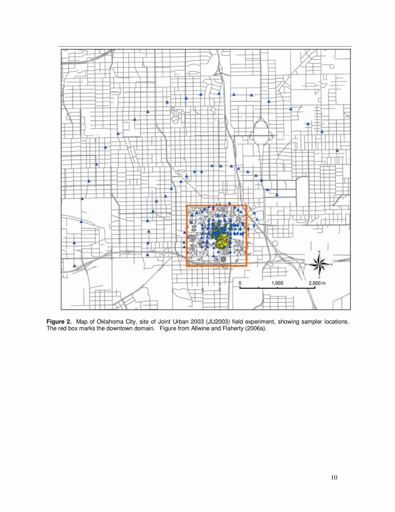
SF6 releases was planned to allow sufficient time for a “gap” to appear between the released clouds, so they could be easily distinguished. The SF6 concentrations analyzed here were reported as 30-min averages over a 6-h period during each night. The 6-h duration was planned to allow sufficient time to capture concentration data from all three releases. However, for some of the light-wind IOPs, the cloud from the third release had not reached the most distant (6 km) arc before the sampling ended. 4.2 Joint Urban 2003 (JU2003) in Oklahoma City The Joint Urban 2003 (JU2003) field experiment was conducted in Oklahoma City (Figure 2), and is described in detail by Allwine and Flaherty (2006a). JU2003 consisted of ten IOPs, where each IOP involved three SF6 tracer releases of 30-min duration and intense observations over an 8-h period (Allwine et al. 2004, Clawson et al. 2005). The current study addressed daytime IOPs 3, 4, and 6 and nighttime IOPs 7, 8, 9, and 10. IOP 5 was not considered after it was discovered that it was anomalous because of low mixing depths caused by a nearby thunderstorm complex (White

3

et al., 2009). IOP 1 and 2 were not considered as they were pilot tests. An IOP was conducted only if the wind speed and direction were suitable to ensure that the tracer plume would pass over the array of samplers, which were generally located to the north of the downtown area. Samplers were placed on a rectilinear grid in the downtown area at distances less than 1 km from the source, and on three concentric arcs (at 1, 2, and 4 km) to the north of the downtown area. The current evaluations used the concentrations averaged over 30 min from the National Oceanic and Atmospheric Administration (NOAA) Air Resources Laboratory-Field Research Division (ARL-FRD) samplers (Clawson et al. 2005). Only near-surface samplers were used in the current study. The continuous releases of SF6 tracer gas, at rates of about 2-5 g s-1, were from point sources at a height of about 1.5 m within or just upwind of the built-up downtown area. The releases during IOPs 3, 4, 6, and 7 were from the Botanical Gardens site. The Westin Hotel site was used for IOP 8, and the Park Avenue site was used for IOPs 9 and 10. The average building height (hb) is about 25 m in the downtown area. We considered seven distance arcs for arc-maximum comparisons, where three arcs are well-defined at 1, 2, and 4 km from the source. In the downtown area where samplers were on a rectangular grid, Hanna et al. (2007) subjectively assigned each surface sampler to one of the four effective arc distances of 0.2, 0.37, 0.62, and 0.85 km. One of JEM’s meteorological input options for JU2003 was a single representative wind vector, consisting of a wind speed and a wind direction. The wind direction is important for paired-in-space comparisons, since performance measures are likely to be poor if the assumed wind direction is about 40 deg or more different from the observed plume direction. For JU2003, the average wind speed (the scalar average) and wind direction were based on taking the average over almost 100 downtown anemometers (Hanna et al., 2007). Britter and Hanna (2003) point out that in the low to mid portion of the urban canopy layer (i.e., at z < hb, or about 25 m for Oklahoma City), the wind speed varies less than in the upper portion of the canopy, and thus an average value can be quite useful. To check the choice of wind directions, a comparison was made between the assumed average wind direction for each release trial and the observed plume direction, as determined by drawing a straight line through the middle of the set of samplers where significant SF6 concentrations were observed (Hanna and Baja, 2009). For the 21 JU2003 release trials investigated here, the mean bias between the observed plume and average wind directions was only 2 deg and the root mean square error was about 10 deg.

4.3 Madison Square Garden (MSG05) in Manhattan The MSG05 field experiment (Allwine and Flaherty 2006b, Watson et al. 2006, Hanna et al., 2006) was part of the Urban Dispersion Program (UDP). The science goals for MSG05 were to increase understanding of flow and dispersion in deep urban canyons and of rapid vertical transport and dispersion in recirculating eddies adjacent to very tall buildings in a large urban area. MSG05 took place on 10 and 14 March 2005. Allwine and Flaherty (2006b) and Allwine (2007) describe the experiment in general and give some of the preliminary results. Watson et al. (2006) describe the tracer releases and sampling methodology. Hanna et al. (2006) present some comparisons of five different Computational Fluid Dynamics (CFD) model applied to MSG05, and Hanna et al. (2007) and Hanna and Zhou (2010) discuss the wind and turbulence observations. The average building heights are found to be about 60 m in the MSG area, and there are several buildings with heights above 150 or 200 m within a few blocks. For example, the One Penn Plaza (OPP) building just north of MSG has a height of 223 m (see Figure 3). Both MSG05 IOP days were marked by similar wind speeds (about 5 m s

-1) and directions (WNW

to NNW) at rooftop. Temperatures were also similar, slightly below 0.0 C, during both IOPs. Both experiments took place during the daytime, between 7 am and 12:30 pm EST, with partly-cloudy skies. The MSG05 field experiments included concurrent one-hour duration releases of six different perfluorocarbon tracer gases, from five point sources near street-level (at z = 1.5 m) on the sidewalk at the four corners of MSG, and just north of OPP (see Figure 3). Note that, for each release trial, two PFTs were released from one location for quality control. There were 20 street-level and seven rooftop PFT sampler locations. Watson et al. (2006) describe the details of the PFT methods used for MSG05 and Allwine and Flaherty (2006b) review the PFT part of the experiment in their comprehensive summary of MSG05. There are three major advantages of PFTs over other types of tracers – 1) the global backgrounds of most PFTs are very low, 2) the samplers can measure concentrations down to parts per quadrillion (i.e., 1 ppq = 10

-15 parts per

part volume), and 3) multiple PFTs can be released simultaneously and sampled and distinguished by the same sampler. Thus small amounts of PFT gas can be released and still be detected above the global background. And different PFTs can be released at the same time and their individual concentrations detected by the same sampler. For MSG05, six PFTs were used. Even though they have high molecular weights, they act like neutral or passive gases once they are emitted to the atmosphere because their concentrations are

4

so low. Each release was from a height of 1.5 m and was of duration one hour. During each IOP day, there were two releases, starting at about 9 am and about 11:30 am. The exact timing, locations, and release mass are given in Table 2. Thus, even though there were only four release periods during the two days, there were 24 sets of tracer data due to the six PFTs released during each period. Each sampler collected the PFTs in 10 adsorption tubes during each day. The samples were analyzed in the laboratories at BNL and QA/QC procedures applied (see Watson et al., 2006). Similar comprehensive analyses were carried out with the sampling data for all four urban field experiments discussed in this paper. As a representative example from the four urban field experiments, Table 3 gives the background concentrations and the derived uncertainty (expressed as a standard deviation, or Stdev) for each PFT. Also listed are the Level of Detection (LOD) and the Level of Quantification (LOQ), which are assumed to equal three and ten times the Stdev, respectively. It is necessary to subtract the background concentration from observations to properly represent the tracer plume. Allwine and Flaherty (2006b) chose to be conservative in estimating the background for removal by defining it as the measured background plus the Stdev rather than as just the measured background. After removing the background, the final step in determining “background-adjusted” values is to set all negative values to zero. Of the six PFTs released, five gave “good” data. However, one of the PFTs, PECH, was determined to have too much uncertainty and was therefore not used in subsequent analyses. In addition, as recommended by Allwine and Flaherty (2006b), our analysis used a conservative approach for determining background-adjusted values that are significantly different from zero. That is, only those adjusted observed final concentrations that exceeded the LOQ (10 Stdev) were used in our analysis. 4.4 Midtown 2005 (MID05) in Manhattan The Midtown Manhattan 2005 (MID05) field experiment (Allwine and Flaherty 2007, Watson et al. 2007, Clawson et al. 2007) is the UDP’s second major field campaign following MSG05. In addition to improving understanding of flow and dispersion in deep urban street canyons, MID05 also studied outdoor-indoor-subway exchange mechanisms. MID05 took place in August 2005 in Midtown Manhattan in New York City. Allwine and Flaherty (2007) give an overview of the field experiment. Clawson et al. (2007) and Watson et al. (2007) describe the SF6 and PFT sampling systems, respectively. MID05’s study domain consisted of a

2 × 2 km area to the south of Central Park (see Figure 4). MID05 was much more complicated in terms of tracer release locations as these locations sometimes shifted between IOPs. MID05 consisted of six IOPs, all conducted from 6 AM to noon local time. Each IOP further consisted of three 30-min tracer releases, each beginning at 6, 8, and 10 AM EST. During each IOP, six PFTs and SF6 were released simultaneously from different locations. The five PFTs analyzed here are PDCH, PMCP, PTCH, PDCB, and PPCH. Table 4 contains a summary of weather conditions during the six IOP days and the locations of the releases. The tracer release locations indicate the relative direction on Figure 4 (e.g., SW refers to the SW portion of the domain and CR and CR are near the center of the domain). Our analysis mainly used the street-level integrating samplers shown in Figure 4 for JEM’s results validation. These samplers roughly form an 8 × 8 grid, or four “concentric” squares, approximated centered around the CL and CR release locations. 5. METHODS Our published evaluations of HPAC-Urban and JEM with the four urban field experiment observations over the past ten years have used a variety of methods. There are several common themes, though. The comparisons always use qualitative tools such as scatter plots, as well as quantitative performance measures. The performance measures in the BOOT statistical model evaluation method (Hanna 1989, Chang and Hanna 2004) are always used. Assume that X = C/Q (concentration normalized by the emission rate) in the following definitions: Fractional Mean Bias

)XX/()XX(FB popo +−= 2 (1)

Normalized Mean Square Error

)X*X/())XX((NMSE popo2

−= (2)

Geometric Mean

))Xln()Xlnexp((MG po −= (3)

Geometric Variance

))XlnX((lnexpVG po2

−= (4)

Fraction of Xp within a factor of two of Xo

FAC2 (5) In addition, the median, average, and maximum of Xo and Xp are often listed in summary tables.

5

Subscripts p and o refer to predicted and observed, and the overbar represents an average. Besides the performance measures suggested in Chang and Hanna (2004) and listed above, our JEM evaluations include the Normalized Absolute Difference, NAD, which mainly applies to paired-in-space comparisons. It has been used for over two decades by the U.S. Environmental Protection Agency (EPA) in regional ozone model evaluations and has recently been discussed in detail by Warner et al. (2004). It is essentially an extension to the figure-of-merit-in-space (FMS) metric used by the team who evaluated over 20 models using the Chernobyl and the ETEX data (e.g., Klug et al. 1992, Girardi et al. 1998). In its original definition based on actual values of predictions and observations, NAD equals the average absolute difference between Co and Cp, divided by the sum of the mean of Co and Cp. However, in this study we used the “threshold-based” NAD. In this case, NAD equals AF/(AF+AOV), where AF is the average of the numbers of sampling locations where the model gives false-positive (Cp > T and Co < T) and false-negative (Cp < T and Co > T) predictions, AOV is the number of sampling locations where model predictions and observations are both above the threshold (Cp > T and Co > T), and the threshold is arbitrarily taken to be 3 times the instrument detection limit. NAD would equal zero for a perfect model, and would approach 1.0 for a model that always overpredicted or underpredicted by a great deal. For some analyses involving evaluations of predictions paired in space and time with observations, all data are included, even if Co and/or Cp were less than the LOQ. As an example, Table 4 listed the LOQ for each PFT used in MSG05. This allows false positives (Cp>LOQ and Co<LOQ), false negatives (Cp<LOQ and Co>LOQ), and “zero-zeros” (Cp<LOQ and Co<LOQ) to be included. When calculating NAD, all data are included. But for evaluations involving the use of the performance measures in equations (1) through (5), pairs of model predictions and observations were included in the comparison only if both the predicted and observed concentration exceeded the LOQ (i.e., 10 times the Stdev). This is because some of the performance measures “blow up” for C = 0. For MSG05, this restriction resulted in over half of the street-level and aloft samplers not being used in the comparisons at all. For the independent validation and verification (IV&V) of the dispersion model component of JEM, our BOOT model evaluation software was used (Hanna 1989 and Chang and Hanna 2004). However, the DoD requires that acceptance criteria be set for anything going through the IV&V process. Chang and Hanna (2004) reviewed many evaluation exercises, involving many models and many types of observations, and suggested some preliminary acceptance criteria based on some standard performance measures. These were used

in evaluating JEM with five rural field experiments as reported by Chang et al. (2007). Model performance for urban applications is not expected to be as good as that for rural applications due to variability introduced by buildings. Therefore, it was recommended that the model acceptance criteria for urban applications be relaxed by roughly a factor of 2 from those for non-urban cases.

• |FB| < ~67%, i.e., the mean bias < a factor of ~2 • NMSE < ~6, i.e., the random scatter < ~2.4 times the mean • FAC2 > ~30%, i.e., the fraction of Cp within a factor of two of Co • NAD < ~50%, i.e., the fractional area for errors, < ~50%

Note that FB, NMSE, and FAC2 are based on arc-maximum comparisons; and NAD is based on threshold-based paired-in-space comparisons. A comprehensive acceptance criterion is defined as being met if at least half of the performance measure criteria are met for least half of the field experiments considered. 6. RESULTS FOR HPAC-URBAN Results are summarized for JU2003, MSG05, and MID05 for HPAC version 5.0 SP1. Chang et al. (2005) describe HPAC-Urban evaluations for U2000, but that exercise used an early version of the urban model in HPAC, and we have not repeated the exercise with version 5.0. Figure 5 is a scatter plot, for JU2003, of paired in space and time HPAC predictions for the UDM option coupled with the UPW meteorological input option and for the daytime IOPs. It is seen that, although there is little mean bias, there is much scatter. Less than half of the predictions are within a factor of two of the observations although more than half are within a factor of five. For daytime IOPs (3, 4, and 6), UDM with the BDF, AVG, and UPW meteorological options has slightly lower bias and scatter, and slightly higher FAC2. MSS with all meteorological options does well with low bias and scatter except for a few high concentrations (factor of 5 to 10) near the source. A few bugs were found in the way UDM interacts with SWIFT. For night time IOPs (7, 8, 9, and 10) an overprediction bias of about a factor of 2 exists. The results for the MEDOC meteorological option show the least bias, lowest scatter and highest FAC2 at night (all greater than 50%). Because it is not influenced by the SWIFT diagnostic meteorological model, MSS shows better performance. However, the same large overpredictions at a few nearby samplers were found during the night as during the day. Figures 6 and 7 are scatter plots, for MSG05, of paired in space and time HPAC predictions for input of a single rooftop meteorological observation (option SNG) and for the UC and MSS options, respectively. It is seen that there is much scatter,

6

although there are a few points near the solid line that indicates perfect agreement. Most of the points indicating good agreement are from samplers 1 through 4, which are at 200 to 400 m downwind, roughly along the line of the rooftop wind direction. The few highest observed C/Q values are predicted within about a factor of 2. There is not much obvious difference in performance between the three meteorological input options (SNG, UPW, and MEDOC) for any of the urban models. At MSG05, no model option simulates anything other than 0.0 concentrations at samplers 3 and 4 at the top of the One Penn Plaza building (about 229 m). However, the observed C/Q averaged 1 to 3 µs/m

3. This is about 1 to 3 % of the C/Q at street-

level next to OPP and about 10 to 30 % of the C/Q at street level at distances of 200 to 400 m. To summarize the HPAC-Urban performance at MSG05, the UC, UDM and MSS urban options have similar statistical performance (e.g., FAC2 about 0.2 to 0.4 at best, and relative mean bias about a factor of 2). The performance is not much different for the three meteorological options. The best agreement is for the four downwind surface samplers (1, 2, 3, and 4) at distances of 200 to 400 m east of MSG. The model options have as many false negatives as “hits”, but few false positives, implying the predicted plume is too narrow. All models underpredict at the samplers at z = 233 m on the OPP roofs (observed is 5 % of that at street level). HPAC-Urban was also evaluated with the MID05 data by Hanna et al. (2009a). However, the scatter plots and specific results are not given here because of restrictions on release of the concentration observations. In general, the evaluation results were similar to those for JU2003 and MSG05, with similar mean bias and scatter, similar underpredictions of rooftop concentrations, and similar lack of differences among the three urban model options and three meteorological input options. 7. RESULTS FOR JEM JEM was evaluated for all four urban field experiments by Chang and Hanna (2010). An overview of the results from the point of view of the acceptance criteria is given by Hanna et al. (2010). As an example of a scatter plot, Figure 8 shows the observed and predicted arc-max concentrations for U2000 for the JEM urban models UDM and UC and for the upwind meteorological inputs from the Raging Water (RGW) site. RGW is often used as the primary input for models applied to U2000. Table 5 is an example of the summary tables prepared in order to more easily “see” whether the acceptance criteria were satisfied. The table is for the MSG05 surface samplers and for one of the six PFTs used as a tracer. There are three wind input options and two urban dispersion model options

(UC and UDM). Grey shading indicates that the urban acceptance criterion defined in Section 5 was met and no shading indicates that it was not. It is easy to see that there are more grey blocks than unshaded blocks, which suggests that the comprehensive acceptance measure is greater than 50 % and therefore the JEM dispersion model is “acceptable” for this field experiment and tracer. Table 6 provides a summary (across each field experiment and all model options, input conditions and tracers) of the number of cases where each performance measure satisfied its respective acceptance criterion. Only surface samplers are included. Overall, more than half of the time the acceptance criteria proposed above were met (but just barely). As a result, the comprehensive acceptance measure exceeds 50 % and JEM’s performance is considered acceptable for urban applications. The JEM evaluations suggest the following conclusions: For urban field data sets, JEM’s performance is understandably worse due to complexities introduced by buildings. The urban acceptance criteria are set to be about a factor of 2 “less stringent” than the rural values. For near-surface samplers not in the near-field, JEM’s performance is within the urban acceptance criteria for about half of the combinations tested. Based on FAC2, the use of UDM in JEM seems to give better results than the UC option. No meteorological input option is consistently better than other options. There are too many meteorological and urban algorithm options available, which would create challenge to most users. As a result, there should be recommendations for model’s consistent use. Judgment is withheld for rooftop samplers, where nearly all models and meteorological input options underpredicted; and for near-field samplers, where nearly all overpredicted. Model improvements are needed in those areas. We mainly focused on results validation here and in Chang and Hanna (2010), but other IV&V components are also important. For example, detailed scientific reviews of the HPAC/SCIPUFF and UDM technical documents have also been completed 8. LIMITATIONS The model acceptance criteria themselves are somewhat arbitrary, and a more valid and widely-recognized set might result via an expert elicitation process, including a workshop. Clearly the evaluation results depend on the quality and extent of the field experiment and on the scenario being studied. Another issue is that it is not helpful if nearly all models fail the tests (or the converse – if nearly all models pass). We also find that using more onsite data or high-resolution mesoscale meteorological outputs does not necessarily guarantee better model performance. It is clear that HPAC and JEM did not do as well for rooftop

7

and near-field (~within one building height) samplers. These cases are outside UDM’s applicability and were therefore not included in the statistics. ACKNOWLEDGEMENTS This research has been sponsored by the Defense Threat Reduction Agency (DTRA), The JEM Program Office and the National Science Foundation. The DTRA program manager is Rick Fry and the JEM program manager is Thomas Smith. The authors appreciate the discussions of the PFT data with Jerry Allwine and Julia Flaherty of the Pacific Northwest National Laboratory, and guidance concerning the SF6 data provided by Kirk Clawson of NOAA’s Field Research Division. REFERENCES Allwine, K.J., 2007: Field Studies for Validation of Urban Dispersion Models: Current Status and Research Needs. Report No. PNNL-SA-58392 Presented at AGU 2007 Fall Meeting, San Francisco, CA, 14 pp. Allwine, K.J., and J.E. Flaherty, 2006a: Joint Urban 2003: Study Overview and Instrument Locations, PNNL-15967, Pacific Northwest National Laboratory, Richland, WA, 92 pp. Allwine, K.J. and J.E. Flaherty, 2006b: Urban Dispersion Program MSG05 Field Study: Summary of Tracer and Meteorological Measurements, PNNL-15969, Pacific Northwest National Laboratory, Richland, WA, 27 pp. (The complete data set is available on a separate CD). Allwine, K.J. and J.E. Flaherty, 2007: Urban Dispersion Program Overview and MID05 Field Study Summary, PNNL-16696, Pacific Northwest National Laboratory, Richland, WA, 63 pp. (The complete meteorological data set is available on a separate CD). Allwine, K.J., M. Leach, L. Stockham, J. Shinn, R. Hosker, J. Bowers and J. Pace, 2004: Overview of Joint Urban 2003 – An Atmospheric Dispersion Study in Oklahoma City, Preprints, Symposium on Planning, Nowcasting and Forecasting in the Urban Zone. American Meteorological Society, January 11-15, 2004, Seattle, Washington, available at www.ametsoc.org. Allwine, K.J., J.H. Shinn, G.E. Streit, K.L. Clawson and M. Brown, M., 2002: Overview of Urban 2000, A multiscale field study of dispersion through an urban environment. Bull. Am. Meteorol. Soc., 83, 521-536.

Britter, R.E. and S.R. Hanna, 2003: Flow and dispersion in urban areas. Annu. Rev. Fluid Mech. 35, 469-496. Chang, J.C., Z. Boybeyi, H.Tang, G. Cervone, J. Bakosi, S. Hanna, E. Hendrick, L. Santos, and J. Bowers, 2007: Independent Verification and Validation of Joint Effects Model. Prepared for Naval Surface Warfare Center, Dahlgren Division. 191 pp. Chang, J.C., and S.R. Hanna, 2004: Air quality model performance evaluation. Meteorol. and Atmos. Phys., 87, 167-196. Chang, J.C. and S.R. Hanna, 2010: Independent Results Validation of JEM for Urban Applications. Final Report prepared for JEM IV&V Program Office, 136 pp. Chang, J.C., S.R. Hanna, Z. Boybeyi and P. Franzese, 2005: Use of Salt Lake City Urban 2000 data to evaluate the Urban-HPAC model. J. Appl. Meteorol. 44 (5), 485-501. Clawson, K.L., R.G. Carter, D. Lacroix, C. Biltoft, N. Hukari, R. Johnson, J. Rich, S. Beard and T. Strong, 2005. Joint Urban 2003 (JU03) SF6 Atmospheric Tracer Field Tests, NOAA Tech Memo OAR ARL-254, Air Resources Lab., Silver Spring, MD, 162 pages. DTRA, 2008: HPAC Version 5.0 SP1 (DVD Containing Model and Accompanying Data Files), DTRA, 8725 John J. Kingman Road, MSC 6201, Ft. Belvoir, VA 22060-6201. Girardi F., G. Graziani, D. van Velzen, S. Galmarini, S. Mosca, R. Bianconi, R. Bellasio, W. Klug, and G. Fraser, 1998: The European Tracer Experiment, EUR 18143 EN, ISBN 92-828-5007-2, Joint Research Centre, European Commission, 106 pp. Hanna, S.R., 1989: Confidence limits for air quality model evaluations as estimated by bootstrap and jackknife resampling methods. Atmos. Environ., 23, 1385-1398.

Hanna, S.R. and E. Baja, 2009: A simple urban dispersion model tested with tracer data from Oklahoma City and New York City. Atmos. Environ. 43, 778-786. Hanna, S.R., E. Baja, J. Flaherty and J. Allwine, 2007: Use of tracer data from the Madison Square Garden 2005 experiment to test a simple urban dispersion model. Paper 4.1, AMS Urban Environ. Conf. www.ametsoc.org Hanna, S.R., R.E. Britter and J.C. Chang, 2010: Observed tracer concentrations in downtown Oklahoma City and Manhattan – Variation with

8

downwind distance and ratios of rooftop to surface concentration. Paper 4.1, AMS 9th Urban Environ. Conf., Keystone, CO. www.ametsoc.org Hanna, S.R., R.E. Britter, and P. Franzese, 2003: A baseline urban dispersion model evaluated with Salt Lake City and Los Angeles Tracer data. Atmos Environ. 37, 5069-5082. Hanna, S.R., M.J. Brown, F.E. Camelli, S. Chan, W.J. Coirier, O.R. Hansen, A.H. Huber, S. Kim and R.M. Reynolds, 2006: Detailed simulations of atmospheric flow and dispersion in urban downtown areas by Computational Fluid Dynamics (CFD) models – An application of five CFD models to Manhattan. Bull. Am. Meteorol. Soc., 87, 1713-1726. Hanna, S.R., J.C. Chang and R.I. Sykes, 2009a: HPAC-Urban and mass-consistent urban model evaluations. Presented at DTRA CBS&T conference, Dallas, TX, November 2009, Two-Page Poster. Hanna, S.R., J.C. Chang, J.M. White and J.F. Bowers, 2007: Evaluation of the HPAC dispersion model with the JU2003 tracer observations. Paper 10.1, AMS 7

th Conference on the Urban

Environment. www.ametsoc.org.

Hanna, S., P. Fabian, J. Chang, A. Venkatram, R. Britter, M. Neophytou and D. Brook, 2004: Use of Urban 2000 field data to determine whether there are significant differences between the performance measures of several urban dispersion models. Paper 7.3, AMS 5th Conference on Urban Environment, www.ametsoc.org Hanna, S.R., R.I. Sykes. J.C. Chang, J. White and E. Baja, 2008: Urban HPAC and a simple urban dispersion model compared with the JU2003 field data. Proceedings, 12

th Conference on

Harmonization of Air Pollution Models used for Regulatory Purposes, Oct 2008, Cavtat, Croatia. Hanna, S.R., R.I. Sykes. S. Parker, J.C. Chang, J. White and E. Baja, 2009b: Urban HPAC and a simple urban dispersion model compared with the MSG05 tracer observations in Manhattan. Paper 18.2, AMS 8th Conference on Urban Environment, Phoenix, AZ. www.ametsoc.org Hanna, S.R., R.I. Sykes. S. Parker, J.C. Chang and J. White, 2009c: Urban HPAC 5.0 evaluations with JU2003 and MSG05 data. Presented at TTCP-CBD Group technical Panel 9 Annual Meeting, DSTO, Melbourne, Australia, February, 31 page PPT file. Hanna, S.R., J. White, J. Troiler, R. Vernot, M. Brown, H. Kaplan, Y. Alexander, J. Moussafir, Y. Wang, C. Williamson, J. Hannan and E. Hendrick, 2011: Comparisons of JU2003 observations with

four diagnostic urban wind flow and Lagrangian particle dispersion models. Submitted to Atmos. Environ. Hanna, S.R., J. White and Y. Zhou, 2007: Observed winds, turbulence, and dispersion in built-up downtown areas in Oklahoma City and Manhattan, Boundary-Layer Meteorology, 125, 441-468. Klug, W., G. Graziani, G. Grippa, D. Pierce, and C. Tassone, 1992: Evaluation of long-range atmospheric transport models using environmental radioactivity data from the Chernobyl accident. The ATMES Report, Elsevier Applied Science, London. Sykes, R.I., S. Parker, D. Henn and B. Chowdhury, 2007: SCIPUFF Version 2.3 Technical Documentation. L-3 Titan Corp, POB 2229, Princeton, NJ 08543-2229, 336 pages. Warner, S., N. Platt, and J.F. Heagy, 2004: User-oriented two-dimensional measure of effectiveness for the evaluation of transport and dispersion models. J. Appl. Meteorol., 43, 58-73. Watson, T.B., J. Heiser, P. Kalb, R.N. Dietz, R. Wilke, R. Weiser and G. Vignato, 2006: The New York City Urban Dispersion program March 2005 Field Study: Tracer Methods and Results. BNL-75592-2006, Brookhaven National Laboratory, POB 5000, Upton, NY 11973-5000. Watson, T.B., J. Heiser, P. Kalb, R.N. Dietz, R. Wilke, and J. Adams, 2007: The New York City Urban Dispersion Program August 2005 Field Study: Tracer Methods and Results. BNL-77986-2007, Brookhaven National Laboratory, POB 5000, Upton, NY 11973-5000. [Limited Distribution – “Official Use Only”] White, J.M., J.F. Bowers, S.R. Hanna, and J.K. Lundquist, 2009: Importance of using observations of mixing depths in order to avoid large errors by a transport and dispersion model. J. Atmos. and Oceanic Technol., 26, 22-32. Zhou, Y. and S.R. Hanna, 2007: Along-wind dispersion of puffs released in built-up urban areas. Bound.-Lay. Meteorol. 125, 469-486.

9

Figure 1. Map of U2000 Salt Lake City downtown area, showing locations of SF6 tracer release and samplers, and locations of meteorological instruments.

10

Figure 2. Map of Oklahoma City, site of Joint Urban 2003 (JU2003) field experiment, showing sampler locations. The red box marks the downtown domain. Figure from Allwine and Flaherty (2006a).

11

Figure 3. MSG05 domain in Manhattan, showing PFT sampler locations. Madison Square Garden is the circular building and different PFTs were released from the sidewalks on the four corners around the building. One PFT was released just north of the One Penn Plaza building with the V1-V4 samplers marked. Samplers with labels beginning with V are located above street level on buildings. Figure from Allwine and Flaherty (2006).

12

Figure 4. MID05 domain, showing PFT and SF6 sampler locations. Release locations varied, depending on the expected wind direction. Figure from Allwine and Flaherty (2007).

13

Figure 5. Scatter plot for JU2003 for daytime IOPs for HPAC UDM option, and upwind input meteorology (Wind instrument #15).

14

Figure 6. Scatter plot for MSG05 for HPAC urban model UC option, and single rooftop wind input.

Figure 7. Scatter plot for MSG05 for HPAC urban model MSS option, and single rooftop wind input.

15

Figure 8. Scatter plot for U2000 for arc-max concentrations for JEM urban model UDM (top) and UC (bottom) and the upwind meteorological inputs from the Raging Water (RGW) site.

16

Table 1. Attributes of four urban field experiments. Releases and samplers are at surface.

Field Exp. Location Time of Day Tracers Releases Samplers

U2000 Salt Lake City Night 1 18 ~100, to ~6 km

JU2003 Oklahoma City Day & night 1 21 ~120, to ~4 km

MSG05 New York City Day 5 20 ~20, to ~0.5 km

MID05 New York City Day 6 87 ~160, to ~2 km

Table 2. Example of detailed source information for the first day (March 10) of MSG05. PFT release locations, start times, release durations, and release masses are listed. From Watson et al. (2006), Allwine and Flaherty (2006), and Hanna et al. (2009b).

Modified form of Table 3 of the BNL Tracer Report

Tracer Release Data for March 10, 2005

Release duration was nominally 1hr. Tracer releases were terminated at 10:00 and 12:30.

Release mass was computed using 1 atm and 0 degC, which was similar to ambient conditions.

Tracer mass has an error of +/- 3%

3/10/2005 Tracer Start Release Duration Release Mass

9:00 EST Release Location Time (min) (g)

oc-PDCH A 9:00 60 0.316

PMCP B 9:05 55 4.624

PMCH C1 9:00 60 1.739

i-PPCH C2 9:00 60 0.082

PECH D 9:02 58 0.592

1PTCH E 9:16 44 0.090

3/10/2005 Tracer Start Release Duration Release Mass

11:30 EST Release Location Time (min) (g)

oc-PDCH A 11:30 60 0.320

PMCP B 11:30 60 5.261

PMCH C1 11:30 60 1.777

i-PPCH C2 11:30 60 0.084

PECH D 11:30 60 0.641

1PTCH E 11:30 60 0.123

17

Table 3. Example for MSG05 of careful consideration of tracer backgrounds and uncertainties. Uncertainties are Expressed as a Standard Deviation (Stdev), Level of Detection (LOD = 3 times Stdev), and Level of Quantification (LOQ = 10 times Stdev). From Watson et al. (2006), Allwine and Flaherty (2006) and Hanna et al. (2009b).

PFT Number of Data Points Used

to Determine Background Background

C in ppqv Stdev

in ppqv LOD

in ppqv LOQ

in ppqv

PMCP 239 19 2.2 6.6 22

PMCH 342 17 2.1 6.3 21

ocPDCH 347 3 0.7 2.1 7

iPPCH 401 6 1 3 10

1PTCH 302 3 1.2 3.6 12

PECH 93 1 3 9 30

Table 4. Summary information for MID05 weather observations and tracer release locations. There are three tracer release times each day, at 0600, 0800 and 1000 EST, with 30 min duration.

IOP Date Weather

Met Life

Z=247 m

U (m/s)

Met Life

WD (°)

LGA

U (m/s)

LGA

WD (°) PDCB PDCH PMCP PPCH PTCH SF6

1 8 Aug

Most cloudy

25-28 C

1.8 221 3.1 205 NONE NONE CL SW-1 to SW

CR SW

2 12 Aug

Part cloudy

30 C 1.3

NE, variable

1.3 to

4.7 50 NONE NONE CL

ENE to SE

CR ENE To SE

3 14 Aug

Part cloudy

30-35 C 2.8 230 3.4 210 NONE NONE CL SW CR SW

4 18 Aug

Part cloudy

25 C 4.9 57 5.5 50 NE CR CL S CR CL

5 20 Aug

Cloudy

25-28 C 2.6 185 4.2 175 NE CR CL S CR CL

6 24 Aug

Clear

25 C 4.2 0 4.7 10 NE CR CL S CR CL

18

Table 5. Example of performance measures for JEM for MSG05 street-level samplers for PMCH tracer. Grey-shaded blocks met acceptance criteria and un-shaded blocks did not.

Meteorological Input and Urban Model Option Arc-Max

FB NMSE FAC2

Basic default observations from LGA airport UC 0.210 0.76 0.714

UDM 0.776 1.18 0.250

Single local observed UC 0.155 1.27 0.375

UDM 0.740 0.92 0.625

MEDOC (MM5) UC -0.749 4.93 0.143

UDM 0.533 0.38 0.625

Table 6. Summary showing the number out of all of the cases considered where the acceptance criteria were met for JEM, to be compared with the comprehensive acceptance criterion of 50 %.

Performance Measures

Field Data Set FB NMSE FAC2 NAD

U2000 7 of 10 5 of 10 10 of 10 9 of 10

JU2003 2 of 8 1 of 8 8 of 8 8 of 8

MSG05 7 of 18 14 of 18 11 of 18 12 of 18

MID05 6 of 24 14 of 24 17 of 24 10 of 24

Total 22 of 60 34 of 60 46 of 60 39 of 60