Complexity Results and Reconstruction Algorithms for Discrete Tomography
University of California, Los Angeles
Electrical Engineering Department
3D Tomography – Algebraic Reconstruction
Algorithm Implementation
Comprehensive Project Report for Master Degree
Non-thesis Option
by
Haibo Chen
Advisor: Professor Dejan Markovic
Winter 2014
Abstract
In this project, our goal is to complete algorithm implementation and optimization on CPUs
and GPUs for benchmark comparison against the original MATLAB version. And in future, our
implementation can be used to compare against FPGAs.
The whole project contains two steps: two-month literature review and two-month algorithm
implementation with MATLAB, C and CUDA coding. By reading papers and prior MS projects
and thesis, I get the basic knowledge of tomography background, how different algorithms work
and what is the tradeoff between them. And thus my task is specified to implement the two most
widely used iterative algebraic reconstruction algorithms, i.e., SIRT and SART. Simulation results
have given us a clear picture of the speed and reconstruction image quality using such techniques.
Table of Contents
1. Introduction ........................................................................................................................ 1
1.1 Computed Tomography – Image Projection ...................................................... 1
1.2 Motivation of Algebraic Reconstruction Techniques .......................................... 2
1.3 CPU and GPU Architectures ................................................................................ 3
2. Problem Formulation and Hardware Configuration ..................................................... 4
3. SIRT Implementation ........................................................................................................ 5
3.1 Iterative Algorithm of SIRT ................................................................................. 5
3.2 Implementation SIRT with C ............................................................................... 6
3.3 Implementation SIRT with CUDA .................................................................... 11
3.4 SIRT: Results and Analysis ................................................................................ 14
4. SART Implementation..................................................................................................... 15
4.1 Iterative Algorithm of SART ............................................................................. 15
4.2 Implementing SART with C .............................................................................. 17
4.3 Implementing SART with CUDA ...................................................................... 19
4.4 SART: Results and Analysis .............................................................................. 20
5. Summary and Future Work ........................................................................................... 22
1 / 24
1. Introduction
1.1 Computed Tomography – Image Projection
Tomography refers to the cross-sectional imaging of an object. And data of this image is
usually collected by illuminating the object from many directions (angles) with some sort of
radiation such as X-rays [1]. Computed Tomography (CT) is one of the primary tomography
imaging techniques. In a CT system, the object is placed at the center of the system. There is also
an array of sources and detectors that rotate about the object at a certain number of different angles.
The source gives radiation towards the detector, and the detector measures the absorption along
the projection path. The more angles of projections are taken, the more reconstruction data are
collected. A larger number of projection angles is supposed to give more accurate reconstruction
image quality, but time required to complete the process is inevitably longer.
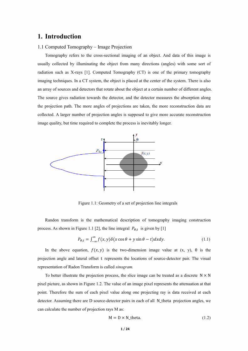
Figure 1.1: Geometry of a set of projection line integrals
Randon transform is the mathematical description of tomography imaging construction
process. As shown in Figure 1.1 [2], the line integral 𝑃𝜃,𝑡 is given by [1]
𝑃𝜃,𝑡 = ∫ 𝑓(𝑥, 𝑦)𝛿(𝑥 cos 𝜃 + 𝑦 sin 𝜃 − 𝑡)𝑑𝑥𝑑𝑦∞
−∞. (1.1)
In the above equation, 𝑓(𝑥, 𝑦) is the two-dimension image value at (x, y), θ is the
projection angle and lateral offset t represents the locations of source-detector pair. The visual
representation of Radon Transform is called sinogram.
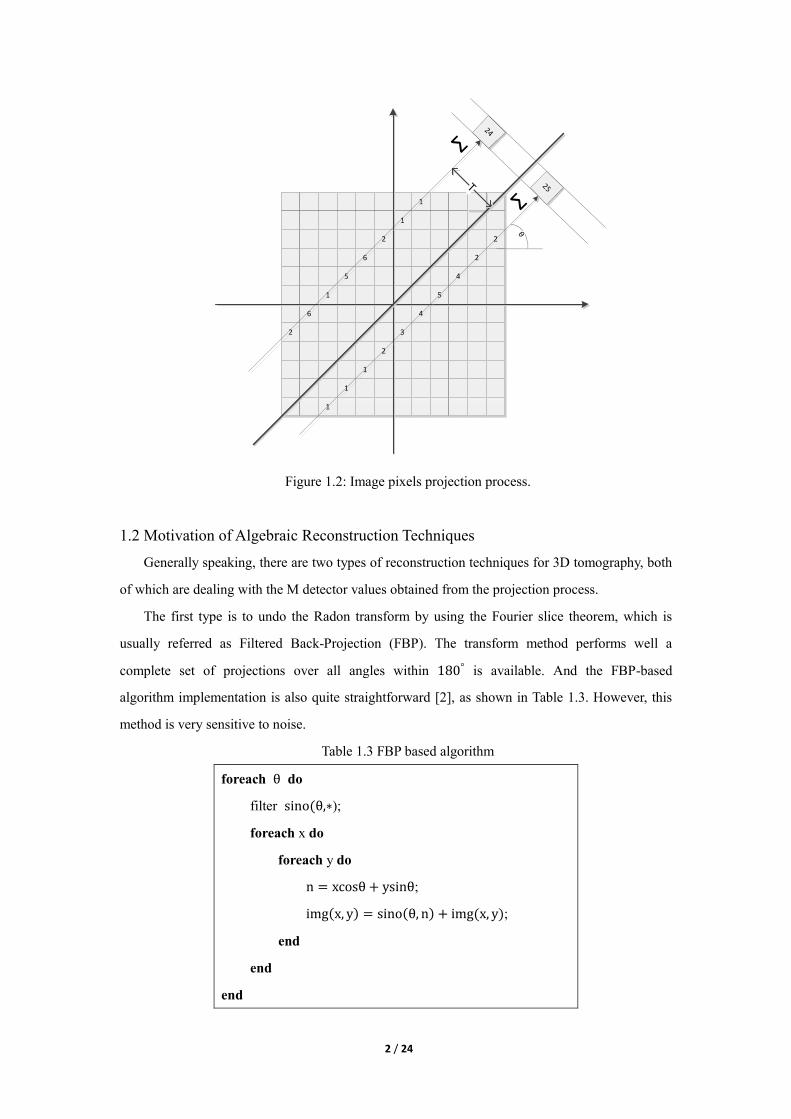
To better illustrate the projection process, the slice image can be treated as a discrete N × N
pixel picture, as shown in Figure 1.2. The value of an image pixel represents the attenuation at that
point. Therefore the sum of each pixel value along one projecting ray is data received at each
detector. Assuming there are D source-detector pairs in each of all N_theta projection angles, we
can calculate the number of projection rays M as:
M = D × N_theta. (1.2)
2 / 24
1
24
1
2 2
6 2
5 4
1 5
6 4
2 3
2
1
1
1
25
Σ
Σ T
θ
Figure 1.2: Image pixels projection process.
1.2 Motivation of Algebraic Reconstruction Techniques
Generally speaking, there are two types of reconstruction techniques for 3D tomography, both
of which are dealing with the M detector values obtained from the projection process.
The first type is to undo the Radon transform by using the Fourier slice theorem, which is
usually referred as Filtered Back-Projection (FBP). The transform method performs well a
complete set of projections over all angles within 180° is available. And the FBP-based
algorithm implementation is also quite straightforward [2], as shown in Table 1.3. However, this
method is very sensitive to noise.
Table 1.3 FBP based algorithm
foreach θ do
filter sino(θ,∗);
foreach x do
foreach y do
n = xcosθ + ysinθ;
img(x, y) = sino(θ, n) + img(x, y);
end
end
end
3 / 24
In the second category of algebraic methods, there are three most popular algorithms:
Algebraic Reconstruction Technique (ART), Simultaneous Iterative Reconstruction Technique
(SIRT) and Simultaneous Algebraic Reconstruction Technique (SART). There are three major
advantages of using algebraic methods [3]. First, they do not require a complete set of projections
over the whole angle range. They are also more stable under noise. Moreover, such methods can
utilize a priori information during reconstruction process. However, due to the iterative processing
method applied, such algorithms are computationally less competitive against transform methods.
The general idea of algorithm design for algebraic methods is summarized as in Table 1.4:
Table 1.4 Algebraic method based algorithm
foreach iteration k do
foreach subsets do
Apply the updating equation on sinogram volume;
Update current volume;
end
end
Recently, with the development of multi-thread processing GPU technology, the algebraic
methods have become more attractive. In the next section, key differences between CPU and GPU
architectures are introduced.
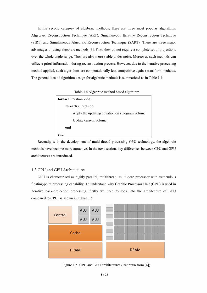
1.3 CPU and GPU Architectures
GPU is characterized as highly parallel, multithread, multi-core processor with tremendous
floating-point processing capability. To understand why Graphic Processor Unit (GPU) is used in
iterative back-projection processing, firstly we need to look into the architecture of GPU
compared to CPU, as shown in Figure 1.5.
Control
Cache
ALU
ALU ALU
DRAM DRAM
ALU
Figure 1.5: CPU and GPU architectures (Redrawn from [4]).
4 / 24
From the above figure, it is clear that with very similar chip areas, GPU provides more
transistors for data processing. And parallel data computations are better supported in a GPU with
its parallel processing threads. Thus the large portion memory access latency in a CPU can be
hidden by calculating instead of accessing memory in a GPU.
In our iterative method for 3D tomography back-projection, the most time consuming step is
matrix-vector multiplication. In GPUs, the large sets of pixels weights and detector data can be
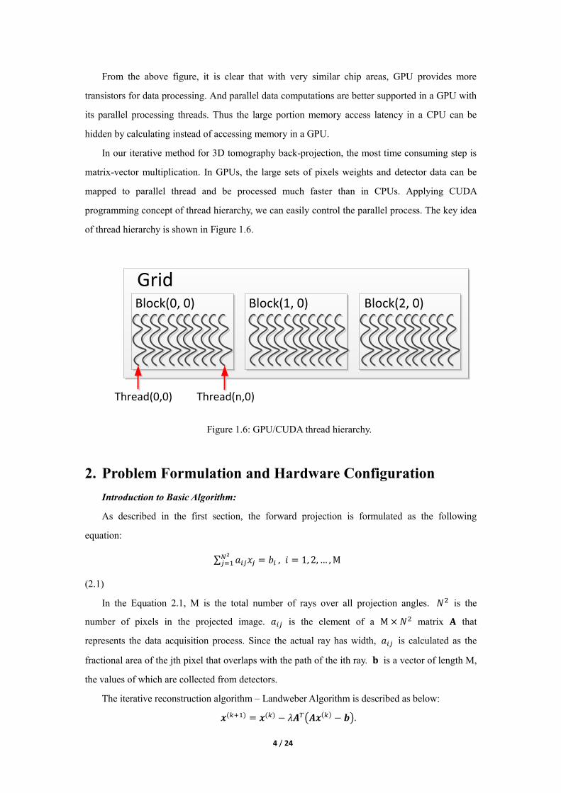
mapped to parallel thread and be processed much faster than in CPUs. Applying CUDA
programming concept of thread hierarchy, we can easily control the parallel process. The key idea
of thread hierarchy is shown in Figure 1.6.
GridBlock(0, 0) Block(1, 0) Block(2, 0)
Thread(0,0) Thread(n,0)
Figure 1.6: GPU/CUDA thread hierarchy.
2. Problem Formulation and Hardware Configuration
Introduction to Basic Algorithm:
As described in the first section, the forward projection is formulated as the following
equation:
∑ 𝑎𝑖𝑗𝑥𝑗 = 𝑏𝑖𝑁2
𝑗=1 , 𝑖 = 1, 2,… ,M
(2.1)
In the Equation 2.1, M is the total number of rays over all projection angles. 𝑁2 is the
number of pixels in the projected image. 𝑎𝑖𝑗 is the element of a M × 𝑁2 matrix 𝐀 that
represents the data acquisition process. Since the actual ray has width, 𝑎𝑖𝑗 is calculated as the
fractional area of the jth pixel that overlaps with the path of the ith ray. 𝐛 is a vector of length M,
the values of which are collected from detectors.
The iterative reconstruction algorithm – Landweber Algorithm is described as below:
𝒙(𝑘+1) = 𝒙(𝑘) − 𝜆𝑨𝑇(𝑨𝒙(𝑘) − 𝒃).
5 / 24
(2.2)
In kth iteration, the image reconstruction value vector 𝒙 is updated by a corrector value. 𝜆 is
a scalar with relaxation factor. If we further introduce the normalization vectors W and V, the
above equation comes to:
𝒙(𝑘+1) = 𝒙(𝑘) − 𝜆𝑽𝑨𝑇𝑾(𝑨𝒙(𝑘) − 𝒃), (2.3)
where W and V are the diagonal matrices of the inverse of row and column sums:
𝑊𝑖 = 𝑊𝑖,𝑖 =1
∑ 𝑎𝑖,𝑗𝑁2
𝑗=1
, 𝑉𝑗 = 𝑉𝑗,𝑗 =1
∑ 𝑎𝑖,𝑗𝑀𝑖=1
.
Both the SIRT and SART algorithms are based on Equation 2.3. And as mentioned, the priori
information in algebraic reconstruction methods refers to the item of 𝑮 = 𝑽𝑨𝑇𝑾 in this equation.
Matrix A is simply about the spatial relation between source-detector pairs and image pixels of
scanned object slices. This information is considered to be unchanged during a 3D tomography
process. Therefore matrix G is stored in CPU or GPU memory prior to starting the iterative
processing operation.
Although derived from the same idea, the main difference between SIRT and SART is the way
they update the sinogram vector 𝐱. Based on the Algebraic Reconstruction Techniques (ART),
SIRT gives less “salt and pepper” noise at the expense of slower convergence [1]. SART aims to
combine faster convergence (ART) and better looking image with less effect of noise (SIRT)
together. The details of both techniques are reported in the following sections.
Hardware Environment:
This project is carried out on the Kodiak Linux server (kodiak.ee.ucla.edu). The CPU is an
Intel Core i7-2600 Quad-Core HT 3.4GHz processor. The GPU is a NVIDIA GeForce GTX 660
graphics card.
3. SIRT Implementation
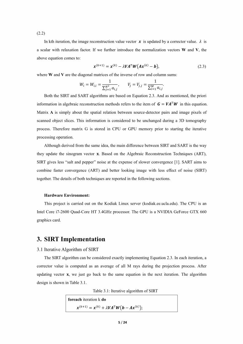
3.1 Iterative Algorithm of SIRT
The SIRT algorithm can be considered exactly implementing Equation 2.3. In each iteration, a
corrector value is computed as an average of all M rays during the projection process. After
updating vector 𝐱, we just go back to the same equation in the next iteration. The algorithm
design is shown in Table 3.1.
Table 3.1: Iterative algorithm of SIRT
foreach iteration k do
𝒙(𝑘+1) = 𝒙(𝑘) + 𝜆𝑽𝑨𝑇𝑾(𝒃 − 𝑨𝒙(𝑘));
6 / 24
end
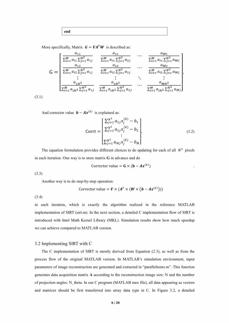
More specifically, Matrix 𝑮 = 𝑽𝑨𝑇𝑾 is described as:
G =
[
𝑎11
∑ 𝑎𝑖1𝑀𝑖=1 ∑ 𝑎1𝑗
𝑁2𝑗=1
𝑎21
∑ 𝑎𝑖1𝑀𝑖=1 ∑ 𝑎2𝑗
𝑁2𝑗=1
⋯𝑎𝑀1
∑ 𝑎𝑖1𝑀𝑖=1 ∑ 𝑎𝑀𝑗
𝑁2𝑗=1
𝑎12
∑ 𝑎𝑖2𝑀𝑖=1 ∑ 𝑎1𝑗
𝑁2𝑗=1
𝑎22
∑ 𝑎𝑖2𝑀𝑖=1 ∑ 𝑎2𝑗
𝑁2𝑗=1
⋯𝑎𝑀2
∑ 𝑎𝑖2𝑀𝑖=1 ∑ 𝑎𝑀𝑗
𝑁2𝑗=1
⋮ ⋮ ⋱ ⋮𝑎
1𝑁2
∑ 𝑎𝑖𝑁2𝑀𝑖=1 ∑ 𝑎1𝑗
𝑁2𝑗=1
𝑎2𝑁2
∑ 𝑎𝑖𝑁2𝑀𝑖=1 ∑ 𝑎2𝑗
𝑁2𝑗=1
⋯𝑎
𝑀𝑁2
∑ 𝑎𝑖𝑁2𝑀𝑖=1 ∑ 𝑎𝑀𝑗
𝑁2𝑗=1 ]
.
(3.1)
And corrector value 𝒃 − 𝑨𝒙(𝑘) is explained as:
Corrt =
[ ∑ 𝑎1𝑗𝑥𝑗
(𝑘)𝑁2
𝑗=1 − 𝑏1
∑ 𝑎2𝑗𝑥𝑗(𝑘)𝑁2
𝑗=1 − 𝑏2
⋮
∑ 𝑎𝑀𝑗𝑥𝑗(𝑘)𝑁2
𝑗=1 − 𝑏𝑀]
. (3.2)
The equation formulation provides different choices to do updating for each of all 𝑁2 pixels
in each iteration. One way is to store matrix G in advance and do
Corrector value = 𝐆 × (𝐛 − 𝑨𝒙(𝑘)) .
(3.3)
Another way is to do step-by-step operation:
Corrector value = 𝑽 × (𝑨𝑇 × (𝑾 × (𝒃 − 𝑨𝒙(𝑘))))
(3.4)
in each iteration, which is exactly the algorithm realized in the reference MATLAB
implementation of SIRT (sirt.m). In the next section, a detailed C implementation flow of SIRT is
introduced with Intel Math Kernel Library (MKL). Simulation results show how much speedup
we can achieve compared to MATLAB version.
3.2 Implementing SIRT with C
The C implementation of SIRT is mostly derived from Equation (2.3), as well as from the
process flow of the original MATLAB version. In MATLAB’s simulation environment, input
parameters of image reconstruction are generated and extracted in “paralleltomo.m”. This function
generates data acquisition matrix A according to the reconstruction image size: N and the number
of projection angles: N_theta. In our C program (MATLAB mex file), all data appearing as vectors
and matrices should be first transferred into array data type in C. In Figure 3.2, a detailed
7 / 24
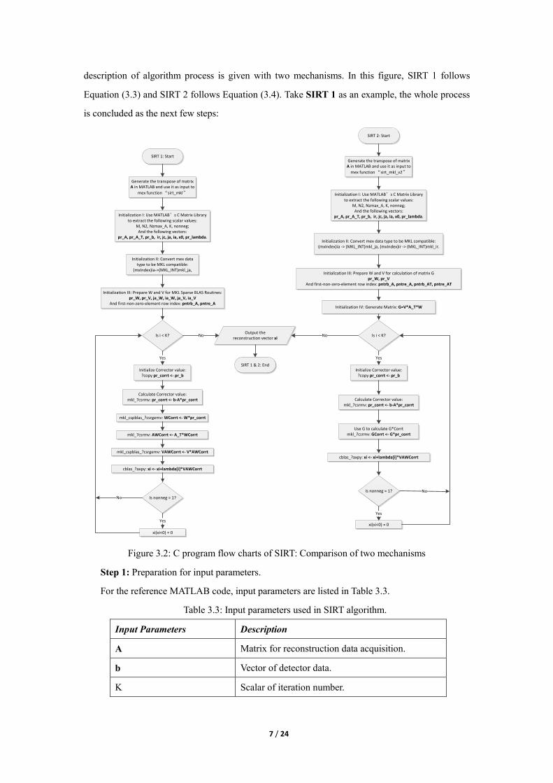
description of algorithm process is given with two mechanisms. In this figure, SIRT 1 follows
Equation (3.3) and SIRT 2 follows Equation (3.4). Take SIRT 1 as an example, the whole process
is concluded as the next few steps:
SIRT 1: Start
Generate the transpose of matrix A in MATLAB and use it as input to
mex function “sirt_mkl”
Initialization I: Use MATLAB’s C Matrix Library to extract the following scalar values:
M, N2, Nzmax_A, K, nonneg;And the following vectors:
pr_A, pr_A_T, pr_b, ir, jc, ja, ia, x0, pr_lambda.
Initialization II: Convert mex data type to be MKL compatible:
(mxIndex)ia->(MKL_INT)mkl_ja,
Initialization III: Prepare W and V for MKL Sparse BLAS Routines:pr_W, pr_V, ja_W, ia_W, ja_V, ia_V
And first-non-zero-element row index: pntrb_A, pntre_A
Is i < K?
Initialize Corrector value:?copy pr_corrt <- pr_b
Calculate Corrector value:mkl_?csrmv: pr_corrt <- b-A*pr_corrt
mkl_cspblas_?csrgemv: WCorrt <- W*pr_corrt
mkl_?csrmv: AWCorrt <- A_T*WCorrt
mkl_cspblas_?csrgemv: VAWCorrt <- V*AWCorrt
cblas_?axpy: xi <- xi+lambda[i]*VAWCorrt
Is nonneg = 1?
xi(xi<0) = 0
Yes
Yes
No
Output the reconstruction vector xi
No
SIRT 1 & 2: End
SIRT 2: Start
Generate the transpose of matrix A in MATLAB and use it as input to
mex function “sirt_mkl_v2”
Initialization I: Use MATLAB’s C Matrix Library to extract the following scalar values:
M, N2, Nzmax_A, K, nonneg;And the following vectors:
pr_A, pr_A_T, pr_b, ir, jc, ja, ia, x0, pr_lambda.
Initialization II: Convert mex data type to be MKL compatible:(mxIndex)ia -> (MKL_INT)mkl_ja, (mxIndex)ir -> (MKL_INT)mkl_ir.
Initialization III: Prepare W and V for calculation of matrix Gpr_W, pr_V
And first-non-zero-element row index: pntrb_A, pntre_A, pntrb_AT, pntre_AT
Initialization IV: Generate Matrix: G=V*A_T*W
Is i < K?No
Initialize Corrector value:?copy pr_corrt <- pr_b
Calculate Corrector value:mkl_?csrmv: pr_corrt <- b-A*pr_corrt
Use G to calculate G*Corrtmkl_?csrmv: GCorrt <- G*pr_corrt
cblas_?axpy: xi <- xi+lambda[i]*VAWCorrt
Is nonneg = 1?
xi(xi<0) = 0
Yes
Yes
No
Figure 3.2: C program flow charts of SIRT: Comparison of two mechanisms
Step 1: Preparation for input parameters.
For the reference MATLAB code, input parameters are listed in Table 3.3.
Table 3.3: Input parameters used in SIRT algorithm.
Input Parameters Description
A Matrix for reconstruction data acquisition.
b Vector of detector data.
K Scalar of iteration number.
8 / 24
x0 Vector of initial reconstruction value.
lambda Vector with relaxation factors.
nonneg Scalar indicator for resetting negative values.
The C version of SIRT also needs the above input parameters. Moreover, as I embedded the
C/Mex function inside the original “sirt.m” for speed comparison purpose, it is also necessary to
generate A’s transpose matrix A_T first before the execution of our C function: “sirt_mkl.c”. One
important reason for doing A’s transpose outside the mex function is that the CPU runs out of
memory easily when calling MATLAB’s “transpose” function in mex file, probably due to some
MATLAB-Mex interface issues.
Step 2: Parameter Initialization in Mex
MATLAB’s C Matrix Library provides functions to extract data from MATLAB’s matrix data
type. Functions used during initialization which are defined by this library are listed in Table 3.4,
and initialized parameters are listed in Table 3.5.
Table 3.4: MATLAB’s C Matrix Library functions used in mex function. [4]
Function Name Description
mxGetM() Get the number of rows in a matrix.
mxGetN() Get the number of columns in a matrix.
mxGetPr(); Access to the data in a matrix in column-major. Return
the pointer to the first element.
mxGetNzmax(); Get the number of non-zero elements in a sparse matrix.
mxGetIr(); Access to the IR array in a sparse matrix.
mxGetJc(); Access to the JC array in a sparse matrix.
Table 3.5: SIRT C: Initialized Parameters in Step 2.
Parameter Description Parameter Description
M Number of rows in A ir Ir array of A
N Number of columns in A jc Jc array of A
Nzmax_A Number of non-zero elements in A ja Ja array of A
K Input: Number of reconstruction iterations ia Ia array of A
nonneg Input: Indicator of resetting negative values x0 Input: vector of initial reconstruction value
9 / 24
pr_A Pointer to data in matrix A in column-major pr_lambda Input: vector with relaxation factors
pr_A_T Pointer to data in matrix A in row-major mkl_ja MKL compatible vector from ja
pntrb_A Vector of row index in CSR format [6] pntre_A Vector of row index in CSR format [6]
Most of the above parameter are accessed or extracted from inputs. Parameters related to A’s
transpose “A_T” are need for two reasons: calculating vector V and doing multiplication of 𝑨𝑇 ×
(𝑾 × (𝒃 − 𝑨𝒙(𝑘))). “pr_A_T” is extracted from input “A_T” using “mxGetPr()”. ir and jc are
index vectors in CSC format defining a sparse matrix. ja and ia are index vectors in CSR format.
Detailed definition of CSC and CSR format can be found in [5] and [6]. These vectors are all
extracted from “A” and “A_T” using “mxGetIr()” and “mxGetJc()”.
Another initialization needed is for convert ja vector of “mxIndex” data type into MKL
compatible “MKL_INT”. Passing “mxIndex” directly to MKL Sparse BLAS routines gives
incorrect results.
Vectors of “pntrb_A” and “pntre_A” are row index vectors defined in CSR format [6] which
are initialized for using MKL’s “mkl_?csrmv” function. Both are set as “MKL_INT” data type.
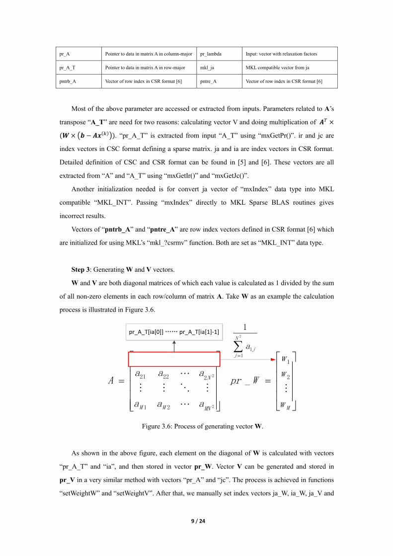
Step 3: Generating W and V vectors.
W and V are both diagonal matrices of which each value is calculated as 1 divided by the sum
of all non-zero elements in each row/column of matrix A. Take W as an example the calculation
process is illustrated in Figure 3.6.
2
2
2
21
22221
11211
MNMM
N
N
aaa
aaa
aaa
A
2
11
1N
jja
pr_A_T[ia[0]] …… pr_A_T[ia[1]-1]
Mw
w
w
Wpr2
1
_
Figure 3.6: Process of generating vector W.
As shown in the above figure, each element on the diagonal of W is calculated with vectors
“pr_A_T” and “ia”, and then stored in vector pr_W. Vector V can be generated and stored in
pr_V in a very similar method with vectors “pr_A” and “jc”. The process is achieved in functions
“setWeightW” and “setWeightV”. After that, we manually set index vectors ja_W, ia_W, ja_V and
10 / 24
ia_V for the purpose of using MKL function “mkl_cspblas_?csrgemv”.
Step 4: Iterative Processing.
The detailed description inside the iteration loop is shown in Figure 3.2: SIRT 1. In each of K
iterations, the vector of reconstruction values xi is updated by a corrector value based on all M
rays. Implementation SIRT 1 follows Equation (3.4). For each step of matrix-vector operation,
Intel Math Kernel Library (MKL) provides very useful BLAS (Basic Linear Algebra Subprograms)
and Sparse BLAS routines that are already optimized for latest Intel processors, also supporting
those with multiple cores [6]. All MKL functions used in the iterative process is listed as follows:
- ?copy is a BLAS Level 1 Routine. It copies input array b to a corrector array: 𝐂𝐨𝐫𝐫𝐭 = 𝐛.
This operation cooperates with the next routine.
- mkl?csrmv is a Sparse BLAS Level 2 Routine. It executes the steps of
𝐂𝐨𝐫𝐫𝐭 = 𝐛 − 𝐀 ∗ 𝐱𝐢 and 𝐀𝐖𝐂𝐨𝐫𝐫𝐭 = 𝐀_𝐓 ∗ 𝐖𝐜𝐨𝐫𝐫𝐭, where vector b is the initialized
corrector array in the previous step.
- mkl_cspblas_?csrgemv is a Sparse BLAS Level 2 Routine. It executes the steps of
𝐖𝐂𝐨𝐫𝐫𝐭 = 𝐖 ∗ 𝐂𝐨𝐫𝐫𝐭 and 𝐕𝐀𝐖𝐂𝐨𝐫𝐫𝐭 = 𝐕 ∗ 𝐀𝐖𝐂𝐨𝐫𝐫𝐭.
- cblas_?axpy is a Sparse BLAS Level 1 Routine. It executes the step of
𝐱𝐢 = 𝐱𝐢 + 𝛌 ∗ 𝐕𝐀𝐖𝐂𝐨𝐫𝐫𝐭.
This mechanism makes step-by-step calculation restricted to only matrix-vector multiplication.
However, it uses vectors W and V as priori information, which adds computation with A_T.
Considering this fact, another mechanism of processing the iteration updating is designed, as
shown with details in Figure 3.2: SIRT 2.
SIRT 2 has almost the same initialization steps as SIRT 1 except that it follows Equation (3.3)
in each iteration updating. Although using G as priori information avoids doing V*A_T*W in
each iteration, the initializing step requires matrix-matrix multiplication, which certainly adds
computation complexity. To verify which of the two mechanisms is more effective, we provide the
same input parameters to both programs. The results are shown in Table 3.7 and Figure 3.8. Note
that only the total time of SIRT’s MATLAB version is measured for reference.
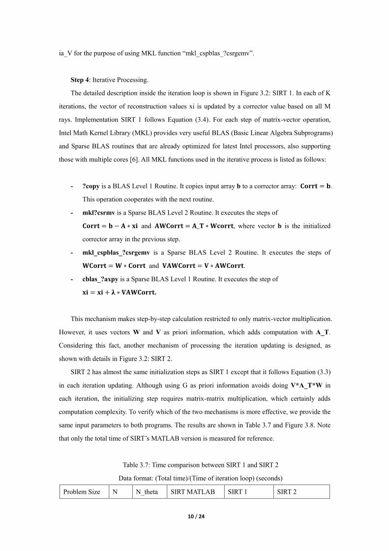
Table 3.7: Time comparison between SIRT 1 and SIRT 2
Data format: (Total time)/(Time of iteration loop) (seconds)
Problem Size N N_theta SIRT MATLAB SIRT 1 SIRT 2
11 / 24
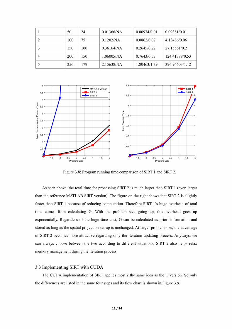
1 50 24 0.01366/NA 0.00974/0.01 0.09381/0.01
2 100 75 0.1202/NA 0.0862/0.07 4.13486/0.06
3 150 100 0.36164/NA 0.2645/0.22 27.15561/0.2
4 200 150 1.06005/NA 0.7643/0.57 124.41388/0.53
5 256 179 2.15638/NA 1.80463/1.39 396.94603/1.12
Figure 3.8: Program running time comparison of SIRT 1 and SIRT 2.
As seen above, the total time for processing SIRT 2 is much larger than SIRT 1 (even larger
than the reference MATLAB SIRT version). The figure on the right shows that SIRT 2 is slightly
faster than SIRT 1 because of reducing computation. Therefore SIRT 1’s huge overhead of total
time comes from calculating G. With the problem size going up, this overhead goes up
exponentially. Regardless of the huge time cost, G can be calculated as priori information and
stored as long as the spatial projection set-up is unchanged. At larger problem size, the advantage
of SIRT 2 becomes more attractive regarding only the iteration updating process. Anyways, we
can always choose between the two according to different situations. SIRT 2 also helps relax
memory management during the iteration process.
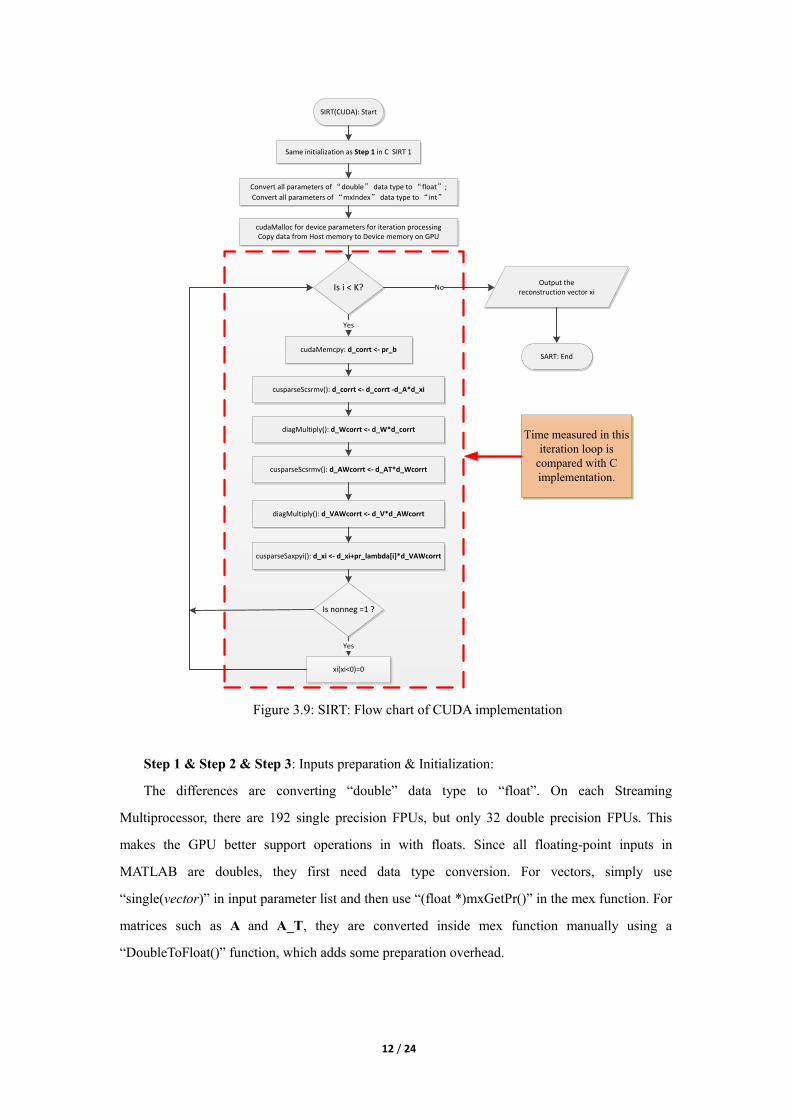
3.3 Implementing SIRT with CUDA
The CUDA implementation of SIRT applies mostly the same idea as the C version. So only
the differences are listed in the same four steps and its flow chart is shown in Figure 3.9.
1 1.5 2 2.5 3 3.5 4 4.5 50
0.5
1
1.5
2
2.5
3
3.5
4
4.5
5
Problem Size
Tota
l R
econstr
uction P
rocess T
ime
MATLAB version
SIRT 1
SIRT 2
1 1.5 2 2.5 3 3.5 4 4.5 50
0.2
0.4
0.6
0.8
1
1.2
1.4
Problem Size
Loop P
rocess T
ime
SIRT 1
SIRT 2
12 / 24
SIRT(CUDA): Start
Same initialization as Step 1 in C SIRT 1
Convert all parameters of “double” data type to “float”;
Convert all parameters of “mxIndex” data type to “int”
cudaMalloc for device parameters for iteration processingCopy data from Host memory to Device memory on GPU
Is i < K?
cudaMemcpy: d_corrt <- pr_b
cusparseScsrmv(): d_corrt <- d_corrt -d_A*d_xi
diagMultiply(): d_Wcorrt <- d_W*d_corrt
cusparseScsrmv(): d_AWcorrt <- d_AT*d_Wcorrt
diagMultiply(): d_VAWcorrt <- d_V*d_AWcorrt
cusparseSaxpyi(): d_xi <- d_xi+pr_lambda[i]*d_VAWcorrt
Is nonneg =1 ?
xi(xi<0)=0
Yes
Yes
Output the reconstruction vector xi
SART: End
No
Time measured in this
iteration loop is
compared with C
implementation.
Figure 3.9: SIRT: Flow chart of CUDA implementation
Step 1 & Step 2 & Step 3: Inputs preparation & Initialization:
The differences are converting “double” data type to “float”. On each Streaming
Multiprocessor, there are 192 single precision FPUs, but only 32 double precision FPUs. This
makes the GPU better support operations in with floats. Since all floating-point inputs in
MATLAB are doubles, they first need data type conversion. For vectors, simply use
“single(vector)” in input parameter list and then use “(float *)mxGetPr()” in the mex function. For
matrices such as A and A_T, they are converted inside mex function manually using a
“DoubleToFloat()” function, which adds some preparation overhead.
13 / 24
W and V Generation:
As we have shown in the previous section, the overhead time of initialization is very large
compared to the core loop in the iterative process. And as we will see in results analysis in the next
section, this overhead is even larger during CUDA initialization on the GPU. Considering these
overheads as pre-stored priori information, they are actually not the primary concern when
measuring how much speed up GPU can achieve over CPU. So W and V are generated in advance
using the same C program and both are used as inputs to our CUDA program.
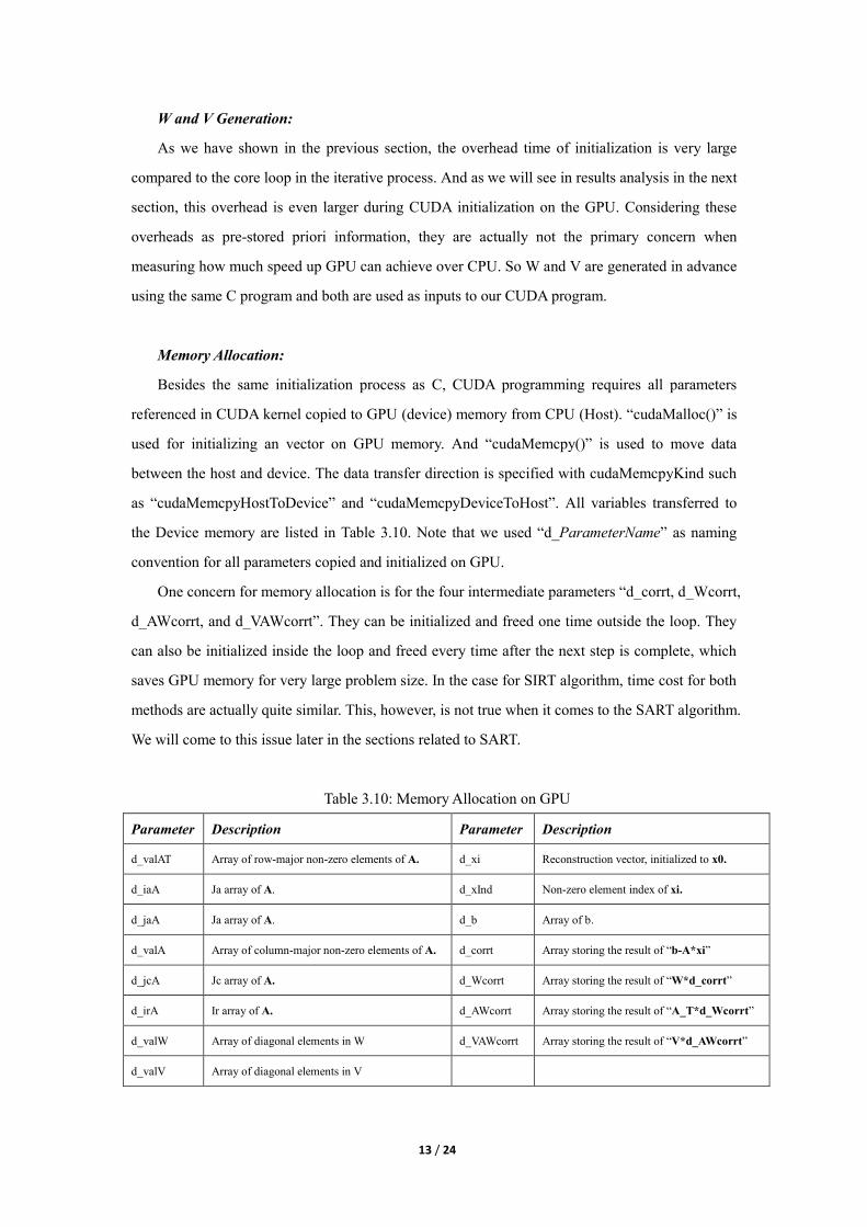
Memory Allocation:
Besides the same initialization process as C, CUDA programming requires all parameters
referenced in CUDA kernel copied to GPU (device) memory from CPU (Host). “cudaMalloc()” is
used for initializing an vector on GPU memory. And “cudaMemcpy()” is used to move data
between the host and device. The data transfer direction is specified with cudaMemcpyKind such
as “cudaMemcpyHostToDevice” and “cudaMemcpyDeviceToHost”. All variables transferred to
the Device memory are listed in Table 3.10. Note that we used “d_ParameterName” as naming
convention for all parameters copied and initialized on GPU.
One concern for memory allocation is for the four intermediate parameters “d_corrt, d_Wcorrt,
d_AWcorrt, and d_VAWcorrt”. They can be initialized and freed one time outside the loop. They
can also be initialized inside the loop and freed every time after the next step is complete, which
saves GPU memory for very large problem size. In the case for SIRT algorithm, time cost for both
methods are actually quite similar. This, however, is not true when it comes to the SART algorithm.
We will come to this issue later in the sections related to SART.
Table 3.10: Memory Allocation on GPU
Parameter Description Parameter Description
d_valAT Array of row-major non-zero elements of A. d_xi Reconstruction vector, initialized to x0.
d_iaA Ja array of A. d_xInd Non-zero element index of xi.
d_jaA Ja array of A. d_b Array of b.
d_valA Array of column-major non-zero elements of A. d_corrt Array storing the result of “b-A*xi”
d_jcA Jc array of A. d_Wcorrt Array storing the result of “W*d_corrt”
d_irA Ir array of A. d_AWcorrt Array storing the result of “A_T*d_Wcorrt”
d_valW Array of diagonal elements in W d_VAWcorrt Array storing the result of “V*d_AWcorrt”
d_valV Array of diagonal elements in V
14 / 24
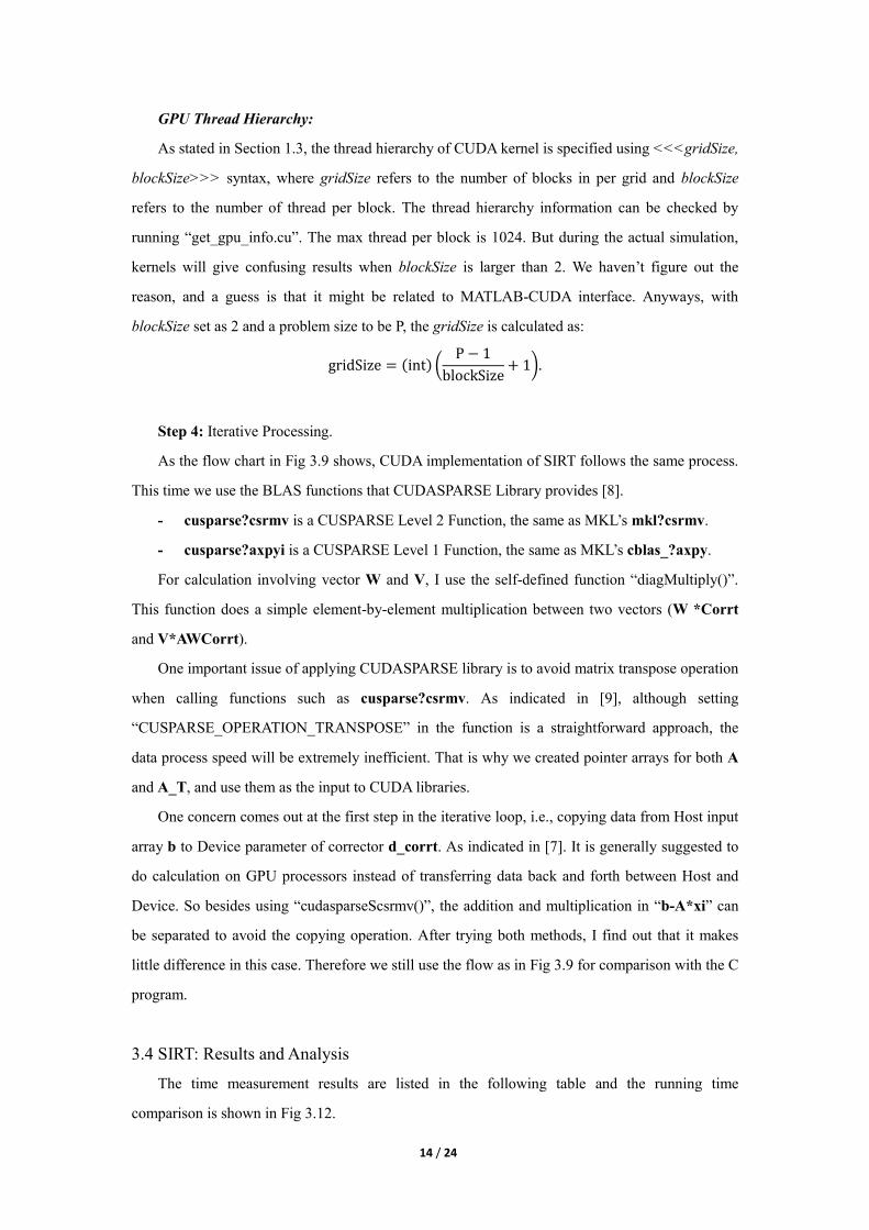
GPU Thread Hierarchy:
As stated in Section 1.3, the thread hierarchy of CUDA kernel is specified using <<<gridSize,
blockSize>>> syntax, where gridSize refers to the number of blocks in per grid and blockSize
refers to the number of thread per block. The thread hierarchy information can be checked by
running “get_gpu_info.cu”. The max thread per block is 1024. But during the actual simulation,
kernels will give confusing results when blockSize is larger than 2. We haven’t figure out the
reason, and a guess is that it might be related to MATLAB-CUDA interface. Anyways, with
blockSize set as 2 and a problem size to be P, the gridSize is calculated as:
gridSize = (int) (P − 1
blockSize+ 1).
Step 4: Iterative Processing.
As the flow chart in Fig 3.9 shows, CUDA implementation of SIRT follows the same process.
This time we use the BLAS functions that CUDASPARSE Library provides [8].
- cusparse?csrmv is a CUSPARSE Level 2 Function, the same as MKL’s mkl?csrmv.
- cusparse?axpyi is a CUSPARSE Level 1 Function, the same as MKL’s cblas_?axpy.
For calculation involving vector W and V, I use the self-defined function “diagMultiply()”.
This function does a simple element-by-element multiplication between two vectors (W *Corrt
and V*AWCorrt).
One important issue of applying CUDASPARSE library is to avoid matrix transpose operation
when calling functions such as cusparse?csrmv. As indicated in [9], although setting
“CUSPARSE_OPERATION_TRANSPOSE” in the function is a straightforward approach, the
data process speed will be extremely inefficient. That is why we created pointer arrays for both A
and A_T, and use them as the input to CUDA libraries.
One concern comes out at the first step in the iterative loop, i.e., copying data from Host input
array b to Device parameter of corrector d_corrt. As indicated in [7]. It is generally suggested to
do calculation on GPU processors instead of transferring data back and forth between Host and
Device. So besides using “cudasparseScsrmv()”, the addition and multiplication in “b-A*xi” can
be separated to avoid the copying operation. After trying both methods, I find out that it makes
little difference in this case. Therefore we still use the flow as in Fig 3.9 for comparison with the C
program.
3.4 SIRT: Results and Analysis
The time measurement results are listed in the following table and the running time
comparison is shown in Fig 3.12.
15 / 24
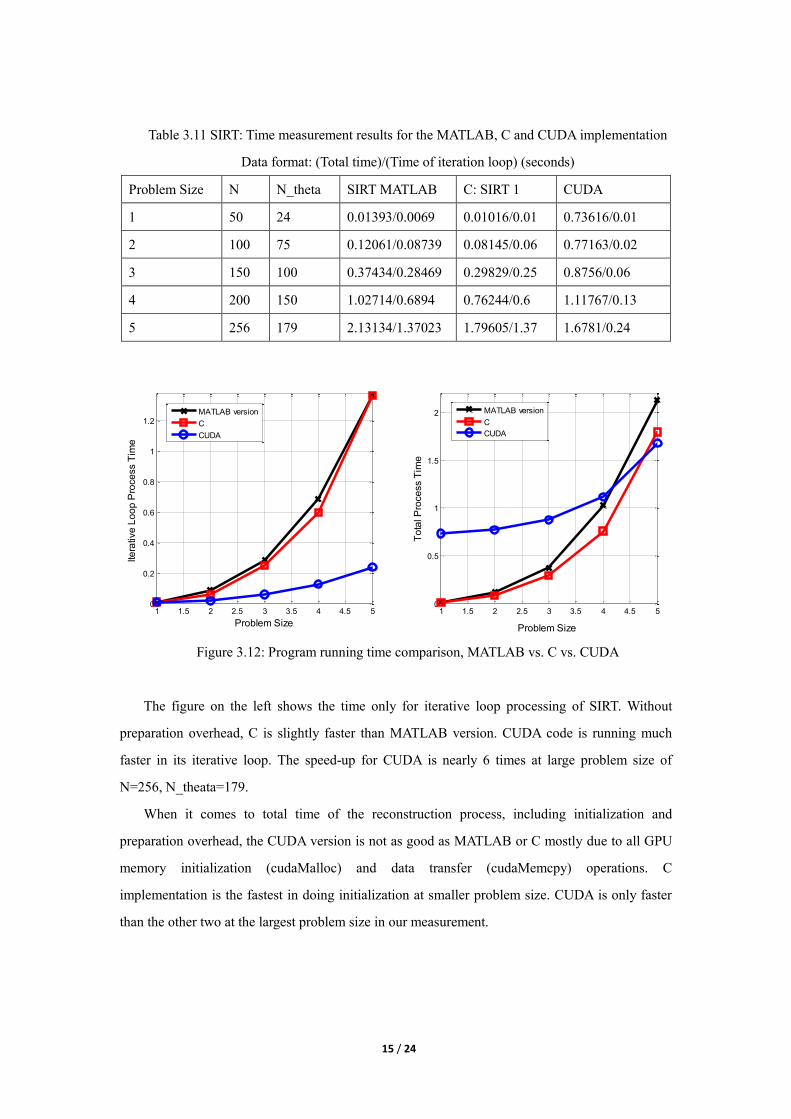
Table 3.11 SIRT: Time measurement results for the MATLAB, C and CUDA implementation
Data format: (Total time)/(Time of iteration loop) (seconds)
Problem Size N N_theta SIRT MATLAB C: SIRT 1 CUDA
1 50 24 0.01393/0.0069 0.01016/0.01 0.73616/0.01
2 100 75 0.12061/0.08739 0.08145/0.06 0.77163/0.02
3 150 100 0.37434/0.28469 0.29829/0.25 0.8756/0.06
4 200 150 1.02714/0.6894 0.76244/0.6 1.11767/0.13
5 256 179 2.13134/1.37023 1.79605/1.37 1.6781/0.24
Figure 3.12: Program running time comparison, MATLAB vs. C vs. CUDA
The figure on the left shows the time only for iterative loop processing of SIRT. Without
preparation overhead, C is slightly faster than MATLAB version. CUDA code is running much
faster in its iterative loop. The speed-up for CUDA is nearly 6 times at large problem size of
N=256, N_theata=179.
When it comes to total time of the reconstruction process, including initialization and
preparation overhead, the CUDA version is not as good as MATLAB or C mostly due to all GPU
memory initialization (cudaMalloc) and data transfer (cudaMemcpy) operations. C
implementation is the fastest in doing initialization at smaller problem size. CUDA is only faster
than the other two at the largest problem size in our measurement.
1 1.5 2 2.5 3 3.5 4 4.5 50
0.2
0.4
0.6
0.8
1
1.2
Problem Size
Ite
rative
Lo
op
Pro
ce
ss T
ime
MATLAB version
C
CUDA
1 1.5 2 2.5 3 3.5 4 4.5 50
0.5
1
1.5
2
Problem Size
To
tal P
roce
ss T
ime
MATLAB version
C
CUDA
16 / 24
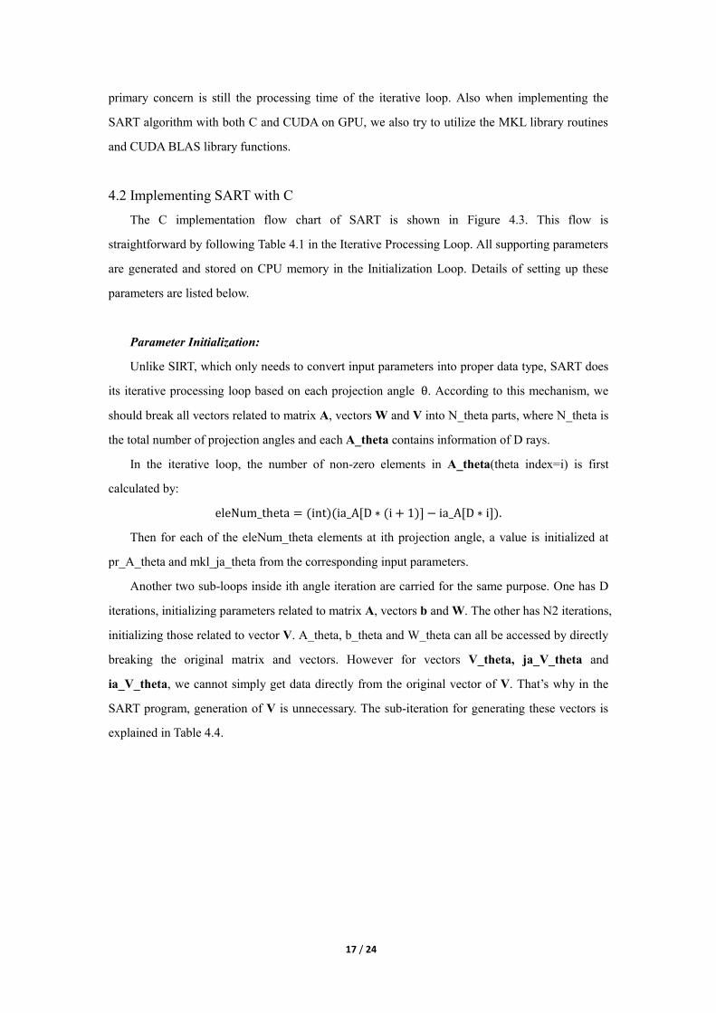
4. SART Implementation
4.1 Iterative Algorithm of SART
The SART algorithm is also derived from Equation (2.3). The difference is that SART applies
an updating period of each projection angle instead of all rays. So based on a revised equation of
(2.3), the SART algorithm is concluded as Table 4.1:
Table 4.1: Iterative algorithm of SART
foreach iteration k do
foreach projection angle θ of D rays do
𝒙(𝜃+1) = 𝒙(𝜃) + 𝜆𝑽𝜃𝑨𝜃𝑇𝑾𝜃(𝒃𝜃 − 𝑨𝜃𝒙(𝜃));
end
end
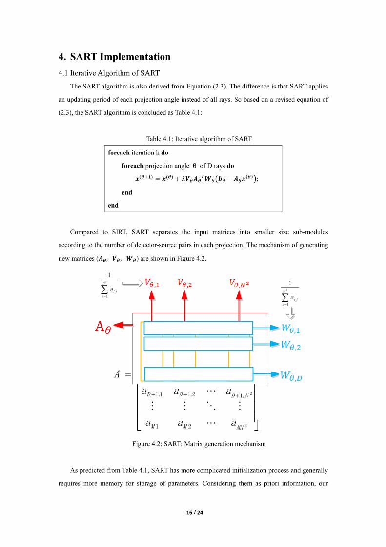
Compared to SIRT, SART separates the input matrices into smaller size sub-modules
according to the number of detector-source pairs in each projection. The mechanism of generating
new matrices (𝑨𝜽, 𝑽𝜃 , 𝑾𝜃) are shown in Figure 4.2.
2
2
2
2
2
21
,12,11,1
21
22221
11211
MNMM
NDDD
DNDD
N
N
aaa
aaa
aaa
aaa
aaa
A
2
1
1N
jija
2
1
1D
iija
Figure 4.2: SART: Matrix generation mechanism
As predicted from Table 4.1, SART has more complicated initialization process and generally
requires more memory for storage of parameters. Considering them as priori information, our
17 / 24
primary concern is still the processing time of the iterative loop. Also when implementing the
SART algorithm with both C and CUDA on GPU, we also try to utilize the MKL library routines
and CUDA BLAS library functions.
4.2 Implementing SART with C
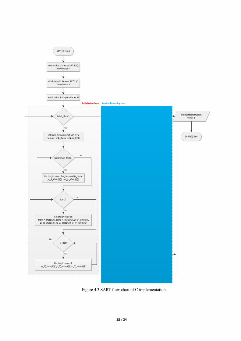
The C implementation flow chart of SART is shown in Figure 4.3. This flow is
straightforward by following Table 4.1 in the Iterative Processing Loop. All supporting parameters
are generated and stored on CPU memory in the Initialization Loop. Details of setting up these
parameters are listed below.
Parameter Initialization:
Unlike SIRT, which only needs to convert input parameters into proper data type, SART does
its iterative processing loop based on each projection angle θ. According to this mechanism, we
should break all vectors related to matrix A, vectors W and V into N_theta parts, where N_theta is
the total number of projection angles and each A_theta contains information of D rays.
In the iterative loop, the number of non-zero elements in A_theta(theta index=i) is first
calculated by:
eleNum_theta = (int)(ia_A[D ∗ (i + 1)] − ia_A[D ∗ i]).
Then for each of the eleNum_theta elements at ith projection angle, a value is initialized at
pr_A_theta and mkl_ja_theta from the corresponding input parameters.
Another two sub-loops inside ith angle iteration are carried for the same purpose. One has D
iterations, initializing parameters related to matrix A, vectors b and W. The other has N2 iterations,
initializing those related to vector V. A_theta, b_theta and W_theta can all be accessed by directly
breaking the original matrix and vectors. However for vectors V_theta, ja_V_theta and
ia_V_theta, we cannot simply get data directly from the original vector of V. That’s why in the
SART program, generation of V is unnecessary. The sub-iteration for generating these vectors is
explained in Table 4.4.
18 / 24
SART (C): Start
Initialization I: Same as SIRT 1 (C): Initialization I
Initialization II: Same as SIRT 1 (C): Initialization II
Initialization III: Prepare Vector W
Is i<N_theta?
Calculate the number of non-zero elements of A_theta: eleNum_theta
Is j<eleNum_theta?
Get the jth value of A_theta and ja_theta:pr_A_theta[i][j], mkl_ja_theta[i][j]
Yes
Yes
Is i<D?
Get the jth value of:pntrb_A_theta[i][j], pntre_A_theta[i][j], pr_b_theta[i][j],
pr_W_theta[i][j], ja_W_theta[i][j], ia_W_theta[i][j]
Is i<N2?
Get the jth value of:pr_V_theta[i][j], ja_V_theta[i][j], ia_V_theta[i][j]
No
Yes
No
Yes
No
Is i<K?
Operation:mkl_?csrmv: pr_corrt(theta) = -A(theta)*xi.
Is j<N_theta?
Yes
Yes
Corrector calculation:vectorAdd(): pr_corrt(theta) = b(theta)-pr_corrt(theta).
mkl_cspblas_?csrgemv: WCorrt(theta)=W(theta)*pr_corrt(theta).
mkl_?csrmv: AWCorrt(theta)=A_T(theta)*Wcorrt(theta).
mkl_cspblas_?csrgemv: VAWCorrt(theta)=V(theta)*AWCorrt(theta).
cblas_?axpy: xi=xi+lambda[i]*VAWCorrt(theta).
Is nonneg=1?
xi(xi<0)=0
Yes
No
No
Output reconstruction vector xi
SART (C): End
Initialization Loop Iterative Processing Loop
Figure 4.3 SART flow chart of C implementation.
19 / 24
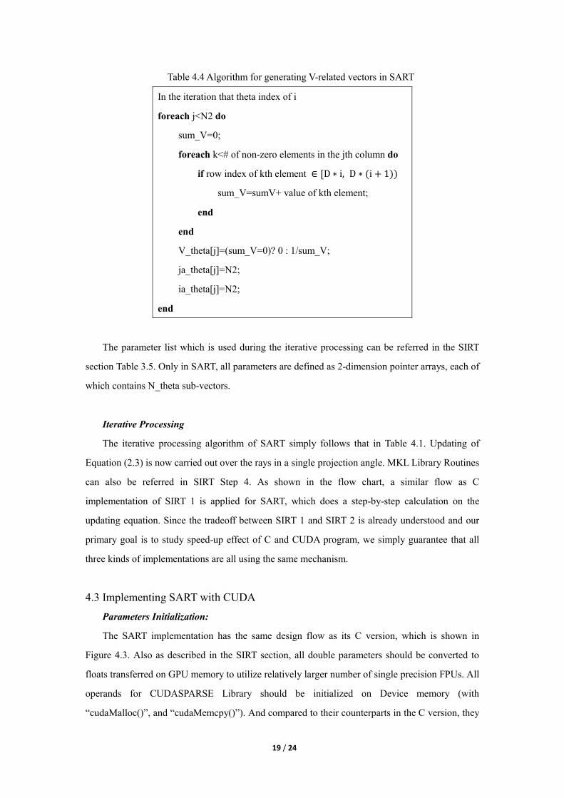
Table 4.4 Algorithm for generating V-related vectors in SART
In the iteration that theta index of i
foreach j<N2 do
sum_V=0;
foreach k<# of non-zero elements in the jth column do
if row index of kth element ∈ [D ∗ i, D ∗ (i + 1))
sum_V=sumV+ value of kth element;
end
end
V_theta[j]=(sum_V=0)? 0 : 1/sum_V;
ja_theta[j]=N2;
ia_theta[j]=N2;
end
The parameter list which is used during the iterative processing can be referred in the SIRT
section Table 3.5. Only in SART, all parameters are defined as 2-dimension pointer arrays, each of
which contains N_theta sub-vectors.
Iterative Processing
The iterative processing algorithm of SART simply follows that in Table 4.1. Updating of
Equation (2.3) is now carried out over the rays in a single projection angle. MKL Library Routines
can also be referred in SIRT Step 4. As shown in the flow chart, a similar flow as C
implementation of SIRT 1 is applied for SART, which does a step-by-step calculation on the
updating equation. Since the tradeoff between SIRT 1 and SIRT 2 is already understood and our
primary goal is to study speed-up effect of C and CUDA program, we simply guarantee that all
three kinds of implementations are all using the same mechanism.
4.3 Implementing SART with CUDA
Parameters Initialization:
The SART implementation has the same design flow as its C version, which is shown in
Figure 4.3. Also as described in the SIRT section, all double parameters should be converted to
floats transferred on GPU memory to utilize relatively larger number of single precision FPUs. All
operands for CUDASPARSE Library should be initialized on Device memory (with
“cudaMalloc()”, and “cudaMemcpy()”). And compared to their counterparts in the C version, they
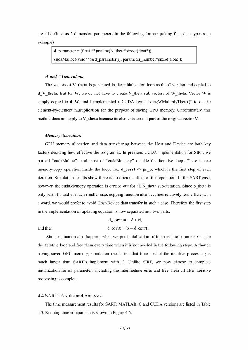
20 / 24
are all defined as 2-dimension parameters in the following format: (taking float data type as an
example)
d_parameter = (float **)malloc(N_theta*sizeof(float*));
cudaMalloc((void**)&d_parameter[i], parameter_number*sizeof(float));
W and V Generation:
The vectors of V_theta is generated in the initialization loop as the C version and copied to
d_V_theta. But for W, we do not have to create N_theta sub-vectors of W_theta. Vector W is
simply copied to d_W, and I implemented a CUDA kernel “diagWMultiplyTheta()” to do the
element-by-element multiplication for the purpose of saving GPU memory. Unfortunately, this
method does not apply to V_theta because its elements are not part of the original vector V.
Memory Allocation:
GPU memory allocation and data transferring between the Host and Device are both key
factors deciding how effective the program is. In previous CUDA implementation for SIRT, we
put all “cudaMalloc”s and most of “cudaMemcpy” outside the iterative loop. There is one
memory-copy operation inside the loop, i.e., d_corrt <- pr_b, which is the first step of each
iteration. Simulation results show there is no obvious effect of this operation. In the SART case,
however, the cudaMemcpy operation is carried out for all N_theta sub-iteration. Since b_theta is
only part of b and of much smaller size, copying function also becomes relatively less efficient. In
a word, we would prefer to avoid Host-Device data transfer in such a case. Therefore the first step
in the implementation of updating equation is now separated into two parts:
d_corrt = −A ∗ xi,
and then d_corrt = b − d_corrt.
Similar situation also happens when we put initialization of intermediate parameters inside
the iterative loop and free them every time when it is not needed in the following steps. Although
having saved GPU memory, simulation results tell that time cost of the iterative processing is
much larger than SART’s implement with C. Unlike SIRT, we now choose to complete
initialization for all parameters including the intermediate ones and free them all after iterative
processing is complete.
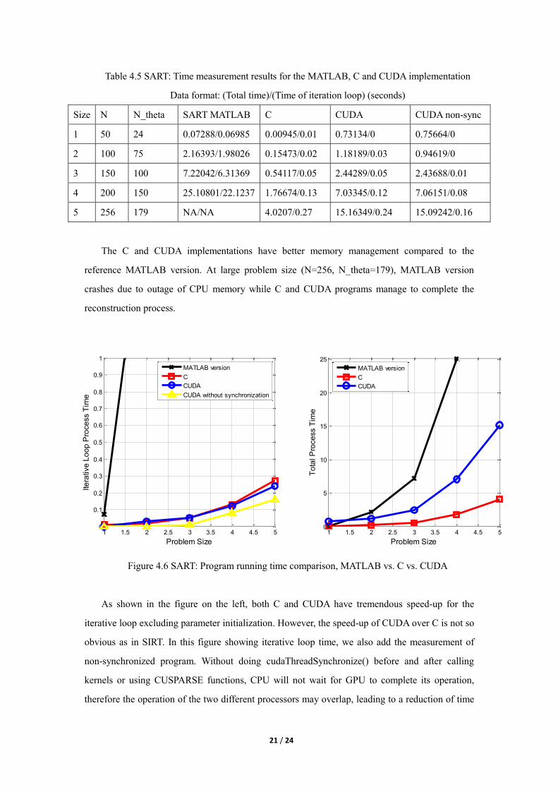
4.4 SART: Results and Analysis
The time measurement results for SART: MATLAB, C and CUDA versions are listed in Table
4.5. Running time comparison is shown in Figure 4.6.
21 / 24
Table 4.5 SART: Time measurement results for the MATLAB, C and CUDA implementation
Data format: (Total time)/(Time of iteration loop) (seconds)
Size N N_theta SART MATLAB C CUDA CUDA non-sync
1 50 24 0.07288/0.06985 0.00945/0.01 0.73134/0 0.75664/0
2 100 75 2.16393/1.98026 0.15473/0.02 1.18189/0.03 0.94619/0
3 150 100 7.22042/6.31369 0.54117/0.05 2.44289/0.05 2.43688/0.01
4 200 150 25.10801/22.1237 1.76674/0.13 7.03345/0.12 7.06151/0.08
5 256 179 NA/NA 4.0207/0.27 15.16349/0.24 15.09242/0.16
The C and CUDA implementations have better memory management compared to the
reference MATLAB version. At large problem size (N=256, N_theta=179), MATLAB version
crashes due to outage of CPU memory while C and CUDA programs manage to complete the
reconstruction process.
Figure 4.6 SART: Program running time comparison, MATLAB vs. C vs. CUDA
As shown in the figure on the left, both C and CUDA have tremendous speed-up for the
iterative loop excluding parameter initialization. However, the speed-up of CUDA over C is not so
obvious as in SIRT. In this figure showing iterative loop time, we also add the measurement of
non-synchronized program. Without doing cudaThreadSynchronize() before and after calling
kernels or using CUSPARSE functions, CPU will not wait for GPU to complete its operation,
therefore the operation of the two different processors may overlap, leading to a reduction of time
1 1.5 2 2.5 3 3.5 4 4.5 50
0.1
0.2
0.3
0.4
0.5
0.6
0.7
0.8
0.9
1
Problem Size
Ite
rative
Lo
op
Pro
ce
ss T
ime
MATLAB version
C
CUDA
CUDA without synchronization
1 1.5 2 2.5 3 3.5 4 4.5 50
5
10
15
20
25
Problem Size
To
tal P
roce
ss T
ime
MATLAB version
C
CUDA
22 / 24
that are measured using clock() in C. Allowing overlapping brings nearly 50% of speed-up for
CUDA implementation. The figure on the right shows how each program performs including
initialization overhead. Both CUDA and C are much faster than MATLAB, but extra GPU
memory allocation and Host-Device data communication makes CUDA program slower than C,
even at large problem size.
5. Summary and Future Work
In this project, we have implemented the SIRT and SART algorithms on CPU and GPU,
serving as benchmark comparisons against the reference MATLAB implementation and also
against FPGAs in the future. Based on equations defined for algebraic reconstruction process, we
manage to execute the iterative process with optimized Sparse BLAS functions both in MKL and
CUDA Libraries.
We have explored different techniques to realize the iterative equation. Initializing the matrix
containing the maximum priori information helps the iterative process run faster, but initialization
takes much more time. Without doing matrix multiplication during initialization, the total time
cost is smaller while the iterative loop is slightly slower.
For SIRT, both C and CUDA achieve speed up in the iterative loop. C can approach 15%-30%
speed-up of total running time over the MATLAB version. CUDA code is especially much faster
during the iterative loop than the other two. Total running time for CUDA is longer due to the
overhead of initialization. With this overhead included, the advantage of CUDA comes up at larger
problem size.
For SART, both C and CUDA achieve huge speed-up compared with MATLAB. However, the
speed-up effect of CUDA is not as remarkable as it is in SIRT. Our judgment is that since SART
breaks input matrices and vectors into smaller sub-modules and SART requires much less iteration
for convergence, GPU’s advantage of operating on large-size matrices greatly decreases.
Based on the progress of this project, we believe that the performance of CUDA
implementation can still be improved by exploring optimization techniques such as memory
sharing and higher-level parallel processing. In future, implementation on FPGAs would be able
to do comparison against the measurements on CPU and GPU to decide possible tradeoffs
[19-20].
23 / 24
Reference
[1] Avinash C. Kak and Malcolm Slaney, “Principles of Computerized Tomographic Imaging”,
IEEE Press, 1988.
[2] H. I. Chen, “An FPGA Architecture for Real-Time 3-D Tomographic Reconstruction”, MS
thesis, UCLA, 2012.
[3] Beata Turonova, “Simultaneous Algebraic Reconstruction Technique for Electron Tomography
using OpenCL”, MS Thesis, Saarland University, 2011.
[4] MathWorks Document Center, http://www.mathworks.com/help/matlab/access-data.html
[5] Timothy. A. Davis, “Direct Methods for Sparse Linear Systems”, Society for Industrial and
Applied Mathematics, 2006.
[6] Intel, “Intel Math Kernel Library-Reference Manual”, MKL 11.0 Update 1.
http://software.intel.com/en-us/articles/intel-math-kernel-library-documentation
[7] Nvidia, “CUDA C Programming Guide”, PG-02829-001_v5.0, October 2012.
http://docs.nvidia.com/cuda/pdf/CUDA_C_Programming_Guide.pdf
[8] Nvidia, “CUSPARSE Library”, v5.0, October 2012.
http://docs.nvidia.com/cuda/pdf/CUDA_CUSPARSE_Users_Guide.pdf
[9] H. Huang, L. Wang, E. Lee and P. Chen, “An MPI-CUDA Implementation and Optimization
for Parallel Sparse Equations and Least Squares (LSQR)”, International Conference on
Computational Science, ICCS 2012.
[10] J. Xu, “A FPGA Hardware Solution for Accelerating Tomographic Reconstruction”, MS
thesis, University of Washington, 2009.
[11] W. Chlewicki, “3D Simultaneous Algebraic Reconstruction Technique for Cone-Beam
Projections”, University of Patras, 2011.
[12] J. Sunnegardh, “Iterative Filtered Backprojection Methods for Helical Cone-Beam CT”,
Linkopoing University, 2009.
[13] J. H. Jorgensen, “Knowledge-Based Tomography Algorithms”, Kongens Lyngby, 2009.
[14] Dreike, Philip, and Douglas P. Boyd. "Convolution reconstruction of fan beam
projections." Computer Graphics and Image Processing 5.4 (1976): 459-469.
[15] Kachelrieß, Marc, Michael Knaup, and Olivier Bockenbach. "Hyperfast Parallel--Beam
Backprojection." Nuclear Science Symposium Conference Record, 2006. IEEE. Vol. 5. IEEE,
2006.
[16] Leeser, Miriam, et al. "Parallel-beam backprojection: an FPGA implementation optimized for
medical imaging." The Journal of VLSI Signal Processing 39.3 (2005): 295-311.
24 / 24
[17] Morton, Ed, et al. "Ultrafast 3D reconstruction for X-ray real-time tomography
(RTT)." Nuclear Science Symposium Conference Record (NSS/MIC), 2009 IEEE. IEEE, 2009.
[18] Gac, Nicolas, et al. "High speed 3D tomography on CPU, GPU, and FPGA."EURASIP
Journal on Embedded systems 2008 (2008): 5.
[19] Ren, Fengbo, et al. "A single-precision compressive sensing signal reconstruction engine on
FPGAs," Field Programmable Logic and Applications (FPL), 2013 23rd International Conference,
pp.1-4, Sept. 2013.
[20] R. Dorrance, F. Ren, and D. Marković, "A scalable sparse matrix-vector multiplication
kernel for energy-efficient sparse-blas on FPGAs," 2014 ACM/SIGDA international symposium
on Field-programmable gate arrays. pp. 161-170, Feb 2014.