A modified algebraic reconstruction technique taking refractioninto account with an application in terahertz tomography

Jens Tepe∗, Thomas Schuster† and Benjamin Littau‡

Key words and phrases. terahertz tomography, nondestructive testing, algebraic reconstruc-tion technique (ART), reflection losses, refractive index, Snell’s law

AbstractTerahertz (THz) tomography is a rather novel technique for nondestructive testing that is particularly suitedfor the testing of plastics and ceramics. Previous publications showed a large variety of conventional algorithmsadapted from computed tomography or ultrasound tomography which were directly applied to THz tomography.Conventional algorithms neglect the specific nature of THz radiation, i. e. refraction at interfaces, reflection lossesand the beam profile (Gaussian beam), which results in poor reconstructions. The aim is the efficient reconstructionof the complex refractive index, since it indicates inhomogeneities in the material. A hybrid algorithm has beendeveloped based on the algebraic reconstruction technique (ART). ART is adapted by including refraction (Snell’slaw) and reflection losses (Fresnel equations). Our method uses a priori information about the interface andlayer geometry of the sample. This results in the “Modified ART for THz tomography”, which reconstructssimultaneously the complex refractive index from transmission coefficient and travel time measurements.

1 Introduction

Terahertz (THz) radiation has become increasingly popular for nondestructive testing of plasticsand ceramics in recent years. With a frequency range between 100 GHz to 10 THz, this radiationis situated between microwaves and infrared light within the electromagnetic spectrum. Thus, interms of the wavelength, THz radiation shows elements of ray character (X-ray CT) as well as ofwave character (ultrasound tomography). As a result, the wave character cannot be completelyneglected. While plastics and ceramics are almost transparent in this frequency range, THzradiation cannot easily penetrate water, metals and conductive materials. Because of its relativelylong wave length compared to X-rays, THz radiation has a limited lateral resolution. However,by using modulated THz radiation, information about both phase and amplitude are available asmeasured data in contrast to conventional tomographic methods [21].

The inverse problem of THz tomography consists of determining dielectric properties (i. e. re-fractive index n and absorption coefficient α) of the material from phase and amplitude infor-mation of the THz radiation, which admits finding material characteristics such as filler contentor the detection of cracks and air cavities. For an overview on the relatively new field of to-mographic methods using THz radiation, see Wang et al. [34], Guillet et al. [17] and Ferguson[14, 15]. Published results can be divided into transmission or reflection tomographic methods∗Department of Mathematics, Saarland University, PO Box 15 11 50, 66041 Saarbrücken, Germany

(jens.tepe@num.uni-sb.de)†Department of Mathematics, Saarland University, PO Box 15 11 50, 66041 Saarbrücken, Germany

(thomas.schuster@num.uni-sb.de), correspondent author.‡German Plastics Center, 97076 Würzburg, Germany (b.littau@skz.de)

1

arX

iv:1

601.

0449

6v1

[m

ath.

NA

] 1

8 Ja

n 20

16

(a) 3D representation of the Gaussian beam (b) Simulation of the electric field of an object consistingof polyethylene (n = 1.51 + 0.023i)

Figure 1: THz radiation for f = 90 GHz propagating from bottom to top as a simulation basedon the Helmholtz equation

based on the available measured data. The adaption of computed tomography methods [20, 25]to the THz range is widely distributed [7, 13, 15, 18, 26, 34]. Here a very simplified propagationalong straight lines is used with the Radon transform as mathematical model. However, physicaleffects such as refraction, diffraction, edge effects and the Gaussian beam profile have an influenceon THz measurements [8]. Some publications consider these effects by adaptations. In [29], Recuret al. presented a filtered backprojection and adapted iterative methods (SART, OSEM) for 3DTHz CT, which considers the intensity distribution of THz rays (Gaussian beam). Mukherjeeet al. only regard cylindric objects, but take Fresnel reflection losses and beam steering lossesinto account, see [23]. Furthermore, Ferguson et al. [15] and Wang et al. [34] reconstruct therefractive index using measurements of the diffracted THz field based on the Helmholtz equation(so-called T-ray Diffraction Tomography, analogous to ultrasound tomography, see [9, 10]).

Due to the long wavelength of THz radiation compared to X-rays (for a frequency of f =0.1 THz, the wavelength is approx. λ = 3 mm), wave phenomena need to be taken into accountin the modeling of the measurement process. On the other hand, a more precise model leads toa computationally more intensive solution. Our task is to find a balance between both.

In the following we present a novel, hybrid algorithm for THz tomography. The algorithmis developed for a tomograph designed for medium-sized companies, which demands a shortruntime. Because of that we search for an efficient solution of the inverse problem by consideringonly dominating effects.

The radiation from a THz source behaves ideally as a Gaussian beam and can be modeled bythe wave equation or, if we are only interested in the intensity, by the Helmholtz equation. Thetransverse intensity profile is well approximated by Gaussian functions (see figure 1a). However,the solution of the Helmholtz equation is very time-consuming. The wave length is significantlysmaller than in the case of acoustic waves, forcing a fine discretization of the domain of interest.This prevents an efficient solution with ultrasound tomography algorithms. Hence, our goal isa new algorithm not based on the solution of wave or Helmholtz equation, but still taking intoaccount the main physical effects. These are primarily transmission, refraction at interfaces,reflection losses and the Gaussian beam profile (see figure 1b). In the following we will neglectthe Gaussian beam profile for the sake of simplicity.

2

The THz tomography system used for this work provides intensity data, analogous to theconventional transmission tomography, as well as (delayed) travel times or path differences, asin ultrasound technology. The reconstruction algorithm described here uses travel time andtransmission data simultaneously to reconstruct the material parameters refractive index andabsorption coefficient. Therefore, we adapt the algebraic reconstruction technique (ART, see[16]) to our physical conditions by taking into account refraction at the interfaces of the objectaccording to Snell’s law and including the reflection losses given by the Fresnel equations. Forthis, we need some a priori information on the object’s interfaces.

This approach is comparable to those in ultrasound CT and ultrasound vector field tomogra-phy, where reconstructions from travel time measurements are improved by considering ray pathswhich take deflection of the ray into account. In ultrasound CT, the ray paths are computedby solving the eikonal equation (ray tracing) [4, 30, 32]. This approach unfortunately requiresa continuously differentiable refractive index and thus a smoothing of any discontinuities of therefractive index at interfaces. Furthermore, it is necessary to solve a nonlinear partial differen-tial equation of first order. Ray tracing algorithms were successfully combined with algebraicreconstruction techniques (ART, SART) [1, 3, 12]. These algorithms work well, if discontinuitiesare smaller than 10 − 20% refractive index deviation [2, 12]. In THz tomography, these devia-tions at interfaces are even higher compared to ultrasound tomography (about 50%). Therefore,refraction at interfaces can be assumed as a dominating effect in THz tomography.

In ultrasound vector field tomography, signals travel along geodesic curves of a Riemannianmetric, which is associated with the refractive index according to Fermat’s principle [31, 27]. Theinverse problem consists of determining the refractive index from integrals along geodesics curvesfrom ultrasound time-of-flight (TOF) measurements. In both, THz tomography and ultrasoundvector field tomography, the ray path resp. geodesic curve depends on the unknown refractiveindex.

The algorithm presented here allows discontinuities in the refractive index and includes thechange of direction of the rays at interfaces by a direct application of Snell’s law.

The paper is organized as follows. In the next section we briefly recall the mathematicalmodel for the 2D THz transmission and travel time tomography. Subsequently, the notation ofthe a priori given interfaces and a brief description of the physical model, especially the Fresnelequations and Snell’s law, will be discussed. In Section 2.3 we derive a description of ray pathsconsidering refraction. Section 3 deals with the development of the new algorithm, beginningwith a brief revision of the conventional ART. Based on ART, we introduce the modified ARTfor THz tomography and its implementation. Eventually, the validation of the modified ARTand its implementation are to be found in section 4 using synthetic as well as real measureddata, comparing our algorithm with the filtered backprojection (FBP) and conventional ART.We conclude the paper with a summary of the main results and an outlook for future work andpotential improvements.

2 The mathematical model of 2D THz tomography

We consider 2D THz transmission and travel time tomography with standard parallel scanninggeometry. The main task is the reconstruction of an object characterized by the complex refractiveindex n : Ω→ C with

n(x) = n(x) + iκ(x), x ∈ Ω, (2.1)

where Ω =x ∈ R2 : ‖x‖ < R

with R > 0 the radius of the considered domain. The real part

n describes the optical path length of the material, whereas the imaginary part κ models thematerial-dependent absorption. The transmission coefficient τ = I/I0 and the path difference

3

d = c0(T −T0) are available as measured data, with I0 the initial intensity, I the intensity at thedetector, T the travel time with and T0 without an object in the ray path and c0 the speed oflight. The real part of the complex refractive index is the quotient of the speed of light c0 andthe propagation speed cM inside the medium,

n(x) =c0

cM (x), x ∈ Ω, cM > 0. (2.2)

This means the (delayed) travel time is physically related to real part of n. The imaginary part

κ(x) = α(x)c0

4πf, x ∈ Ω, f > 0, (2.3)

describes the absorption of the wave by the absorption coefficient α in cm−1 and is connected tothe transmission coefficient τ . Furthermore, we assume that the complex refractive index vanishesoutside the reconstruction region Ω, i. e. n(x) − 1 = 0 and κ(x) = 0, if x /∈ Ω. Let L be thepropagation path of the THz radiation. The ratio of the transmitted intensity I and the initialintensity I0 is connected to the absorption coefficient α via

gabs(L) =

ˆ

L

α(x) dx = ln

(I0

I

)= ln

(1

τ

)(2.4)

according to Lambert-Beer’s law. The path difference is given by

gref(L) =

ˆ

L

(n(x)− 1) dx = d, (2.5)

which follows from subtraction of the path in air with a refractive index of n0 = 1, see [24].Due to refraction at interfaces, THz rays do not necessarily propagate along straight lines.

The rays are rather refracted at interfaces according to Snell’s law. In case of a piecewise constantrefractive index, the propagation path is continuous and consists of piecewise straight lines. Wename the segments of a THz ray between two interfaces as “partial ray” Ll ⊆ L with l = 1, ..., K+1and K the number of intersected interfaces. The first partial ray L1 is parametrized as in X-rayCT until reaching the first interface, see [25, p. 41-42]. Let

Γ : R→ R2, Γ(t) = sω(ϕ) + tω⊥(ϕ) (2.6)

be the parametrization of L1 with distance s ∈ R from the origin, the angle ϕ ∈ [0, 2π), ω(ϕ) =(cosϕ, sinϕ)T and ω⊥ = (− sinϕ, cosϕ)T . Using Γ, the ray is represented by

L1 (ϕ, s) =

Γ(t) : t ∈[−∞, tif1 (ϕ, s)

](2.7)

with tif1 (ϕ, s) the time of the incidence on the first interface (so-called “initial ray”). In X-ray CT,this parameter is usually set to tif1 = ∞. The full ray path depending on refraction is describedin section 2.3. Therefore we first need to take a closer look at a suitable notation of the interfacesand afterwards we briefly describe the relevant physical laws.

2.1 Notation of interfaces

As mentioned before, we would like to use some a priori information. We postulate the knowledgeof the object’s interfaces, i. e. our a priori information contains positions and the normals of theinterfaces of the object. This is quite a strong assumption, but in many cases the (approximate)location of some interfaces is actually known, for example from CAD drawings of the examined

4

object or preliminary testings with an X-ray CT. However, the interfaces of potential defects areunknown. Nevertheless, the knowledge of some interfaces already leads to better reconstructions.

Definition 2.1. An interface is a regular continuously differentiable and injective immersionΞ : [a, b]→ Ω ⊂ R2, fulfilling Ξ

′(σ) = dΞ

dσ 6= 0, ∀σ ∈ [a, b].

The curve has a tangent and a normal n at every point, because the first derivative Ξ′ is

continuous and does not vanish. The tangent vector of Ξ at σ0 ∈ [a, b] is given by

Ξ′(σ0) =

dΞ

dσ

∣∣∣∣σ=σ0

=(ξ′1(σ0), ξ

′2(σ0)

)T, (2.8)

whereby we define the normal vector

n(σ0) =(−ξ′2(σ0), ξ

′1(σ0)

)T, (2.9)

which we will need for Snell’s law. Let K ∈ N be the number of known interfaces Ξk, k = 1, ..., Kof the object. Interfaces may touch or intersect each other as we often have to deal with non-smooth interfaces, e. g. rectangular objects. However, Ξ

′(σ) and hence the normal does not exist

at corners. This case is handled by local smoothing. Let us assume, that

P :=

K⋂ι=1

Ξkι (2.10)

is the shared intersection of K ∈ [1, K] different interfaces Ξkι with kι ∈ [1, K] , ι = 1, ..., K.Then σkι := Ξ−1

kι(P ) ∈ [akι , bkι ] parametrizes the point of intersection on each interface and

nkι(σkι) are the corresponding normals for ι = 1, ..., K. We now compute the normal in P byaveraging

n =

∑Kι=1 nkι(σkι)∥∥∥∑Kι=1 nkι(σkι)

∥∥∥ , (2.11)

which can be interpreted as a mean orientation of the interfaces containing P . This approach setsa normal for the intersection, which occurs by a local smoothing of the corner P (see figure 2).For K = 1 the normal vector is just normalized.

Figure 2: Dealing with corners: the calculated normal for the discontinuity corresponds to thenormal of the smoothed interface at this point

2.2 Refraction and reflection losses

We follow the idea of Mukherjee et. al, see [23], who consider refraction and reflection losses forcylindrical objects with known refractive index for the reconstruction of the absorption coefficient.We generalize this approach for general objects with given interfaces, unknown n and reconstructboth refractive index and absorption coefficient. The propagation of electromagnetic waves atan interface between two different media is influenced by refraction, reflection, diffraction and

5

interface

Figure 3: Snell’s law with normal n of the interface and direction vectors ω⊥l , ω⊥l+1 and −ωl of

the incident, refracted and reflected rays, n1 < n2

scattering. As stated before, we want to neglect diffraction and scattering. Let us consider thetransition of a ray from a medium with refractive index n1 into a medium with refractive indexn2. The change in the direction of propagation of the transmitted part of the THz ray can becalculated according to Snell’s law

n1 sin γ1 = n2 sin γ2, (2.12)

with the angle of incidence γ1 and the angle of refraction γ2 measured from the normal n of theinterface, see [6, p. 38 ff.]. When rays travel from a medium with a higher refractive index n1 toone with a lower refractive index n2, total reflection is possible for a sufficiently large γ1. In thiscase, we have

n1

n2sin γ1 > 1, for n1 > n2 (2.13)

and the radiation is fully reflected. The fraction of the incident radiation that is reflected at theinterface can be described by the Fresnel equations, see [6, p. 38 ff.]. Reflection losses depend onthe polarization of the incident wave, the angle of incident γ1 and refraction γ2 and the refractiveindices. The reflectance of a ray that is polarized perpendicularly to the plane of incidence isgiven by

ρ =

∣∣∣∣ErE0

∣∣∣∣2 =

∣∣∣∣n1 cos γ1 − n2 cos γ2

n1 cos γ1 + n2 cos γ2

∣∣∣∣2 , (2.14)

where E0 resp. Er is the electric field amplitude of the incident resp. reflected partial ray. Analo-gous considerations exist also for parallel polarization. All other polarizations can be representedby a superposition of the linearly perpendicular and linearly parallel case.

2.3 Ray propagation considering refraction

The path of a THz ray L up to reaching the first interface can be described by equation (2.7).The ray is refracted as it transitions into the next medium and the ray direction has to berecalculated according to Snell’s law. We first have to determine the next intersection with aninterface for each (refracted) partial ray Ll. The change in the direction of the ray is calculatedin this intersection. Let the l-th partial ray Ll be given by an angle ϕl and a distance sl,i .e. Ll (ϕl, sl) =

Γl(t) = slωl + tω⊥l : t ∈

[tifl−1, t

ifl

]. Now we calculate the intersections of Ll

with the interfaces and determine the parameter

6

tifl (ϕl, sl) = mint

(t, σ) ∈

(tifl−1,∞

]× [ak, bk] : Γl(t) = Ξk(σ), k = 1, ...,K

, (2.15)

which defines the nearest intersection with an interface in the direction of propagation with l ≥ 1and tif0 = −∞. Let Ξk(σ), k ∈ [1, K] , be the nearest interface and σ the parameter correspondingto tifl in (2.15) of the intersection Ξk(σ) = slωl + tifl ω

⊥l . We can determine the refractive indices

for both sides of the interface, which we need for Snell’s law, by

nl,1 := n(Ξk(σ)− εn

)and nl,2 := n

(Ξk(σ) + εn

), for

⟨ω⊥l , n

⟩≤ 0

nl,1 := n(Ξk(σ) + εn

)and nl,2 := n

(Ξk(σ)− εn

), for

⟨ω⊥l , n

⟩> 0

(2.16)

with the normal n := n(σ) as in (2.11) and an appropriately small ε > 0. The angle of incidenceγl,1 between the direction vector of the incident ray ω⊥l and normal n (see figure 3) can becalculated by the scalar product in R2

γl,1 = arccos∣∣∣⟨ω⊥l , n⟩∣∣∣ (2.17)

and the angle of the refracted ray can be obtained by

γl,2 =

π − γl,1, for nl,1 > nl,2 ∧ γl,1 ≥ arcsin

nl,2nl,1

(total reflection),

arcsinnl,1 sin γl,1

nl,2, otherwise.

(2.18)

The next direction vector ωl+1 can be easily derived by a rotation of ωl := ω (ϕl) around an angleθ = ± (γl,1 − γl,2) with the rotation matrix

Rθ :=

(cos θ − sin θsin θ cos θ

)(2.19)

see figure 4. The sign of θ depends on the orientation of the normal n to the incident ray, see(2.20). After applying angle sum identities, the new angle ϕl+1 and the unit vector ωl+1 arecomputed by

ωl+1 (ϕl+1) :=

=:ϕl+1

ω(︷ ︸︸ ︷γl,1 − γl,2 + ϕl ), for

⟨ω⊥l , n

⟩< 0 ∧

⟨ω⊥l , n

⊥⟩ ≤ 0ω( γl,1 − γl,2 + ϕl ), for

⟨ω⊥l , n

⟩> 0 ∧

⟨ω⊥l , n

⊥⟩ ≥ 0ω( γl,2 − γl,1 + ϕl ), for

⟨ω⊥l , n

⟩≤ 0 ∧

⟨ω⊥l , n

⊥⟩ > 0ω( γl,2 − γl,1︸ ︷︷ ︸

=:θ

+ ϕl ), for⟨ω⊥l , n

⟩≥ 0 ∧

⟨ω⊥l , n

⊥⟩ < 0

. (2.20)

The next distance from the origin sl+1 of partial ray Ll+1 follows directly from the intersectionof the lines (0 + uωl+1) ∩

(Ξk(σ) + tω⊥l+1

)with parameters t and u. We obtain with Ξk(σ) :=

(ξ1, ξ2)T

sl+1 =∣∣∣(0 + uωl+1) ∩

(Ξk(σ) + tω⊥l+1

)∣∣∣ = |cosϕl+1ξ1 + sinϕl+1ξ2| . (2.21)

Consequently, the complete refracted ray path is given by the union

L (ϕ, s) :=

K+1⋃l=1

Γl(t) : t ∈

[tifl−1, t

ifl

](2.22)

7

-Figure 4: Snell’s law and parametrization of a refracted THz ray

of all partial rays Ll (ϕl, sl) defined by (2.20) and (2.21) with an initial direction ϕ = ϕ1 anddistance s = s1, tif0 = −∞, tif

K+1=∞ and K the number of intersected interfaces. K is unknown

at the beginning and depends on the ray path.

Remark 2.2. Please note that determining the ray paths depends on the refractive index n, whichis the unknown quantity in our inverse problem. Therefore, the actual ray paths are also unknownin the beginning and are approached within the reconstruction process.

Problem 2.3. The inverse problem consists in determining the complex refractive index

n(x) = n(x) + iα(x)c0

4πf, x ∈ Ω, (2.23)

from the knowledge of the measured data gabs(ϕi, sj) = ln(

1τ(ϕi,sj)

)and gref(ϕi, sj) = d(ϕi, sj)

of a parallel scanning geometry with (inital) angles ϕi = 2π(i−1)p for i = 1, ..., p and (initial)

distances sj = Rq j, for j = −q, ..., q. As we do not consider straight ray paths, we usually

have gabs(−ϕ, s) 6= gabs(ϕ, s) or gref(−ϕ, s) 6= gref(ϕ, s) in contrast to X-ray CT. So the anglesϕi should be evenly distributed over the interval [0, 2π). Our task is to find the best possibleapproximation of n satisfying

ˆ

L(ϕi,sj)

(n(x)− 1) dx = gref(ϕi, sj) and

ˆ

L(ϕi,sj)

α(x) dx = gabs(ϕi, sj) (2.24)

for i = 1, ..., p and j = −q, ..., q.

8

3 Algorithm development

In the following, we develop a numerical algorithm for the calculation of the complex refractiveindex n(x) = n(x) + iα(x) c0

4πf . Since algorithms based on partial differential equations suchas the wave equation are very time-consuming, an efficient reconstruction shall only considerdominating physical effects. Poor reconstructions, which arise from the application of conven-tional reconstruction algorithms from computed tomography to THz data, are often based on themissing consideration of refraction and reflection losses.

Therefore, we would like to modify ART for THz tomography. This is done by using a prioriinformation (i. e. the knowledge of interfaces) and considering relevant physical laws (Snell’slaw and reflection losses according to Fresnel equations). This results in a method, which takesrefraction as well as transmission into account and determines simultaneously the refractive indexand the absorption coefficient from measurements of path difference and intensity data.

3.1 ART

Our method is based on the classical ART as described in e. g. [25, pp. 128, 137 ff.]. So wefirst give a brief overview of ART. The main idea behind of this method is the application ofKaczmarz’s method to Radon’s integral equation. We search for the solution of the system

ˆ

Lν

f(x) dx = gν , ν = 1, ..., N, x ∈ Ω (3.1)

where Lν := L(ϕν , sν) are straight lines, f a function (refractive index f = n − 1 or absorptioncoefficient f = α), gν := g(ϕν , sν) the measured data (path difference or intensity data) andN = p(2q + 1). Let

Ω ⊂M⋃µ=1

Sµ (3.2)

be a pixel discretization of the domain Ω with pixels Sµ, µ = 1, ...,M . We obtain a linear systemby discretizing f via

f(x) ≈ f(x) =

M∑µ=1

fµχµ(x), x ∈ Ω, (3.3)

with characteristic functions

χµ(x) =

1, if x ∈ Sµ,0, otherwise.

(3.4)

The integral is thus approximated by

ˆ

Lν

f(x) dx ≈M∑µ=1

aνµfµ (3.5)

with aνµ = length (Lν ∩ Sµ). Now, we define aν := (aν1, ..., aνM )T ∈ RM andF = (f1, f2, ..., fM )T ∈ RM . Using the scalar product in RM , we obtain the discrete versionof (3.1),

〈aν , F 〉 = gν , ν = 1, ..., N. (3.6)

We solve this linear system by applying Kaczmarz’s method to (3.6). The iteration then reads as

9

F 0 := F r

F ν = F ν−1 + λgν −

⟨aν , F ν−1

⟩‖aν‖22

aν , ν = 1, ..., N

F r+1 := FN

(3.7)

with relaxation parameter λ ∈ (0, 2), iteration index r = 0, 1, 2, ..., ray index ν and an arbitraryinitial value F 0.

3.2 Modified ART

We modify ART taking refraction into account. This leads to a more sophisticated calculation ofthe projection matrix A = (aνµ)ν=1,...,N,µ=1,...,M . Furthermore, the consideration of Fresnel lossesleads to a correction of the measured intensity data gabs. Both linear systems (for path differenced and transmission coefficient τ) show a similar structure and can be solved simultaneously, usingthe same ray paths for both models, by applying Kaczmarz’s method to get the complex refractiveindex.

3.2.1 Consideration of Fresnel losses

Reflection losses influence the measured transmission coefficient τ by reducing the intensity ofthe transmitted signal in addition to absorption losses. Neglecting reflection losses in the modelwill thus lead to a systematic error in the calculation of the absorption coefficient: the resultingvalues for α will be too high, as a larger absorption coefficient corresponds to smaller transmissioncoefficients. Therefore, our approach will be a correction of the measured intensity data, sothat only absorption losses are considered for the reconstruction of the absorption coefficient.Mukherjee et al. [23] introduced this approach successfully for cylindric objects. We expand thisapproach to arbitrary interfaces and an initially unknown refractive index.

The reflection loss ρ of a single interface is given by equation (2.14). For this purpose, weneed the angle of incident and refraction, which are known from the calculation of the ray pathsaccording to Snell’s law, as well as the refractive indices on both sides of the interface, givenby (2.16). Let K ∈ N be the number of interfaces intersecting the ray path L and ρkι be thereflection loss at interface Ξkι with kι ∈ [1, K] , ι = 1, ..., K. The emitted intensity is reduceddue to the corresponding reflection losses by the factor

Cabs :=K∏ι=1

(1− ρkι) . (3.8)

In addition, the intensity of the ray is reduced by absorption losses according to Lambert-Beer’slaw

a = exp

(−ˆLα dx

). (3.9)

As a consequence, the transmission coefficient

τ = a

K∏ι=1

(1− ρkι) (3.10)

is measured by the receiver. We are now able to correct the measured transmission data (theright hand side of integral equation (2.4)) by

10

gabs = ln

(I0

I

)= ln

(1

a

)= ln

1

τ

K∏ι=1

(1− ρkι)

(3.11)

and obtain data that depends only on the absorption coefficient α.

3.2.2 Consideration of the refracted ray path

Amatrix entry aνµ represents the length of the (refracted) ray ν in pixel µ as in conventional ART.In contrast to ART, we cannot calculate all entries aνµ at once as the path itself is influenced bythe material parameters. Instead, we have to determine first of all the parameter tifl for partial rayLνl (ϕl, sl) (see section 2.3). Then, we calculate aνµ until reaching the nearest interface, determinethe new angle ϕl+1 according to Snell’s law and the reflection loss ρl for the current interface Ξkaccording to Fresnel equations. Afterwards, these steps can be repeated for the next partial rayLνl+1, l = 1, ..., K and ν = 1, ..., N . A pseudo code for calculating the matrix A and the reflectionlosses is given in algorithm 1.

Algorithm 1 Calculating matrix A and the corrected gabs

1: for ν = 1 to N do2: ρ = 0, tif0 = −∞, tif1 = 0, l = 13: while tifl <∞ do4: Calculate tifl by (2.15)5: Calculate aνµ = length of (Lνl ∩ Sµ) for t ∈

[tifl−1, t

ifl

]6: if tifl <∞ then7: Calculate partial ray Lνl+1(ϕl+1, sl+1) by (2.20) and (2.21)8: Calculate reflection losses ρνl at Ξk by (2.14)9: l = l + 110: end if11: end while12: Kν = l − 1;

13: Calculate Cνabs =∏Kν

l=1 (1− ρνl )14: end for15: gνabs = ln

(Cνabsτν

), ν = 1, ..., N

16: return A, gabs

The reconstruction of Re(n) = n has a direct influence on the reconstruction of the absorptioncoefficient α, because the reflection losses are calculated by using the refractive indices of thematerials that share the interface. The remaining steps are identical to ART. We can use thesame matrix A for the reconstruction of both n − 1 and α and thus the calculation of F rref andF rabs takes place in the same loop, speeding up the reconstruction significantly. In the worst case,the complex refractive index is completely unknown and the initial guess is the complex refractiveindex of air, meaning F 0

ref = F 0abs = 0. In this case it makes sense to perform consecutively several

applications of Kaczmarz’s method and use their approximations for an update of the ray paths,calculating a new matrix A and correction value Cabs before the next iteration. This means, wecalculate the first approximation by conventional ART without considering the interfaces andreflection losses and then the next steps follow with modified ART based on this approximation.This update of ray paths based on an initial guess like F 0

ref = 0 was discussed before in [19] and[30], where it was used in the context of reconstructions based on the eikonal equation.

11

3.2.3 Numerical scheme

Let Ψ be the number of applications of Kaczmarz’s method. We can set the number of iterationsψ =

(r1

stop, ..., rΨstop

)and the relaxation parameters for the refractive index λref =

(λ1

ref , ..., λΨref

)and absorption coefficient λabs =

(λ1

abs, ..., λΨabs

)for each iteration. An appropriate choice of ψ

is important, due to the well-known phenomenon of the semiconvergence of iterative methodsfor inverse problems. The stopping indices ristop, i = 1, ..., Ψ, are the respective regularizationparameters of the modified ART and have to be chosen adequately (e. g. by the discrepancy prin-ciple, see [11]). The algorithm for the calculation of an approximation of the complex refractiveindex based on THz data is shown in algorithm 2. Altogether this leads to the numerical schemefor the modified algebraic reconstruction technique as outlined in figure 5.

Algorithm 2 Modified ART for calculating n = n+ iκ

1: Inital values F 0,1ref , F

0,1abs

2: for i = 1 to Ψ do3: Calculate Ai

(F 0,i

ref

)and gabs

(F 0,i

ref

)by algorithm 1

4: r = 05: while r ≤ ristop do6: F 0

ref = F r,iref , F0abs = F r,iabs

7: for ν = 1 to N do

8: F νref = F ν−1ref + λiref

gνref −⟨aν , F ν−1

ref

⟩‖aν‖22

aν

9: F νabs = F ν−1abs + λiabs

gνabs −⟨aν , F ν−1

abs

⟩‖aν‖22

aν

10: end for11: F r+1

ref = FNref , Fr+1abs = FNabs

12: r = r + 113: end while14: F 0,i+1

ref = FNref , F0,i+1abs = FNabs

15: end for16: return n ≈

(1 + F 0,Ψ+1

ref

)+ i(F 0,Ψ+1

abs

c0

2ω

)

Figure 5: Numerical scheme of the modified ART

12

4 Numerical experiments and results

In this section we would like to validate the modified ART using both synthetic and real measureddata. The results show an improvement of the reconstruction obtained by the proposed techniquein comparison to conventional CT methods. The complex refractive index can be reconstructedin more detail and with smaller errors by applying the new algorithm.

First of all we take a look at reconstructions with synthetic and noisy data. Afterwards, wecompare the results obtained by modified ART with those resulting from FBP and conventionalART on the basis of real measured data. Synthetic and real measured data were both recordedfor p = 360 initial angles and 141 distances (meaning q = 70). Therefore one data set consistsof N = 50760 measurements. Furthermore, the number of iterations ψ and the number ofapplications of Kaczmarz’s methods Ψ, i. e. the regularization parameters, were chosen withouta parameter-choice method for the sake of simplicity. The iterations are just terminated whenfurther iterations show no significant improvement, but not yet divergence.

Additionally, we use the a priori information on the position of the interfaces to reset therefractive index outside the object to n − 1 = 0 before each Kaczmarz’s method. Thus theangles of incidence and refraction are calculated more accurately, as the ray is broken at anactual discontinuity of the refractive index. The initial values F 0,1

ref = F 0,1abs = 0 are used for all

reconstructions, therefore the first iteration is equivalent to conventional ART.

4.1 Synthetic data

The first numerical example concerns a circle with a radius of 50 mm, a refractive index of n = 1.4and an absorption coefficient of α = 0.05 cm−1 containing an embedded rectangle with dimensionsof 25 mm×20 mm and n = 1.7, α = 0.25 cm−1. Uniformly distributed noise is added respectivelyto the synthetic transmission coefficient and path difference data, such that the obtained noisydata gε fulfills

‖g − gε‖2 / ‖g‖2 ≤ 0.05 (4.1)

in both cases. As there is no information about n, we perform several applications of Kaczmarz’s

x (mm)

-80 -60 -40 -20 0 20 40 60

y (

mm

)

-60

-40

-20

0

20

40

60

80

1

1.1

1.2

1.3

1.4

1.5

1.6

1.7

(a) Refractive index n(x), x ∈ Ω

x (mm)

-80 -60 -40 -20 0 20 40 60

y (

mm

)

-60

-40

-20

0

20

40

60

80

0

0.05

0.1

0.15

0.2

0.25

0.3

0.35

0.4

(b) Absolute error

Figure 6: Reconstruction of the refractive index based on synthetic data

13

method for the reconstruction as described in section 3.2.3. Here we used Ψ = 5 iterations withthe following parameters:

ψ = (3, 3, 5, 7, 5)λref = (0.01, 0.01, 0.006, 0.002, 0)

λabs = (0.002, 0.004, 0.004, 0.004, 0.003)(4.2)

We perform only a reconstruction of the absorption coefficient α in last iteration (λ5ref = 0). This

approach is reasonable in so far as we use the approximation of the previous iteration step ofthe refractive index n for calculating the reflection losses for the reconstruction of α. Therefore,we can expect an improvement of α in an additional iteration step. Figures 6 and 7 show the

x (mm)

-80 -60 -40 -20 0 20 40 60

y (

mm

)

-60

-40

-20

0

20

40

60

80

0

0.05

0.1

0.15

0.2

0.25

(a) Absorption coefficient α(x), x ∈ Ω

x (mm)

-80 -60 -40 -20 0 20 40 60

y (

mm

)

-60

-40

-20

0

20

40

60

80

0

0.02

0.04

0.06

0.08

0.1

0.12

0.14

0.16

(b) Absolute error

Figure 7: Reconstruction of the absorption coefficient based on synthetic data

reconstructions of the refractive index and the absorption coefficient with the modified ART. Theresults are good in spite of the large jump discontinuities of the refractive index. The absoluteerror is small in large parts of the object (see figures on the right), whereas the the biggest localerrors appear near the interfaces and corners. Hereby, the prerequisite is ensured that modifiedART provides correct results with synthetic data. As we now have to deal with ray paths that canbe arbitrary refracted at interfaces, it is possible that some pixels are less frequently intersectedby the ray paths than others, which causes additional artifacts.

4.2 Comparison with conventional reconstruction methods using real data

The next step is to compare modified ART with conventional ART and FBP based on realmeasured data. In this context, we first give a brief description of the used THz tomograph andthen move on to the reconstructions.

4.2.1 THz tomography system

The measured data were acquired at SKZ 1. A THz tomography system was designed, whichworks on the basis of the FMCW (Frequency Modulated Continuous Wave) principle. Here

1 The German Plastics Center in Würzburg, http://www.skz.de/

14

the frequency of the THz signal is a sawtooth wave in the range of 70 to 110 GHz and allowsmeasurements of intensity and phase. The latter results in the delayed travel time or pathdifference data. Dispersion can be neglected in this operating frequency range and the complexrefractive index can be assumed to be constant [22, 28]. Thus the transmission coefficient andthe path difference are averaged over this frequency band. The optical system consists of twolenses for each receiver and transmitter and is similar to the architecture of a Kepler telescope.The Gaussian beam is focused on the object with a beam waist of about 8 mm.

Remark 4.1. The generation of synthetic data always provides suitable values gabs and gref ,regardless of how strong the rays are refracted. However, the THz system uses just one emitterand one detector, and in the case of strong refraction the transmitted ray may miss the detector,resulting in a transmission coefficient of τ = 0. Better results can often be achieved by sortingout measured data of rays with τ ≤ εmiss and εmiss sufficiently small, meaning neglecting themcompletely for the iterations. It must be taken into account that this case also occurs for strongabsorbers and then leads to a distortion of the reconstruction results.

4.2.2 Block with multiple refractive indices

The next step is to validate our modified ART with a more complex object and real measureddata. Furthermore, we would like to compare the filtered backprojection, conventional ART andmodified ART. For this purpose a test object consisting of different plastic blocks with differentrefractive indices that where glued together forming a block was scanned. Figure 8 shows themeasures and the refractive indices of the object. The conventional ART no longer achieves

Figure 8: Refractive indices and proportions (in mm) of the glued-together block

significant improvements after 15 iterations with λref = 0.005. The results of modified ART areobtained with ψ = (3, 3, 5, 12) and λref = (0.005, 0.01, 0.0075, 0.003). THz rays resulting intransmission coefficients with τ ≤ 0.05 are ignored in both algebraic methods. Furthermore, weused the filtered backprojection with the Shepp-Logan filter and εmiss = 0. The application ofFBP to THz data leads to a very bad reconstruction (see figure 9) with very high values of n atthe outer interfaces. The shape of the object is completely lost and cannot be reconstructed. Thereconstruction of the conventional ART is slightly better (see figure 10). But the outer shape ofthe object also appears too curved and the reconstruction of the refractive index produces veryhigh values especially around the interfaces.

15

x in mm

-60 -40 -20 0 20 40 60

yin

mm

-60

-40

-20

0

20

40

60

1

1.2

1.4

1.6

1.8

2

2.2

2.4

(a) Refractive index n(x), x ∈ Ω

x in mm

-60 -40 -20 0 20 40 60

yin

mm

-60

-40

-20

0

20

40

60

0

0.1

0.2

0.3

0.4

0.5

0.6

(b) Absolute error

Figure 9: Filtered backprojection: reconstruction of the refractive index with real measured data

x (mm)

-60 -40 -20 0 20 40 60

y (

mm

)

-60

-40

-20

0

20

40

60

1

1.1

1.2

1.3

1.4

1.5

1.6

1.7

(a) Refractive index n(x), x ∈ Ω

x (mm)

-60 -40 -20 0 20 40 60

y (

mm

)

-60

-40

-20

0

20

40

60

0

0.1

0.2

0.3

0.4

0.5

0.6

(b) Absolute error

Figure 10: ART: reconstruction of the refractive index with real measured data

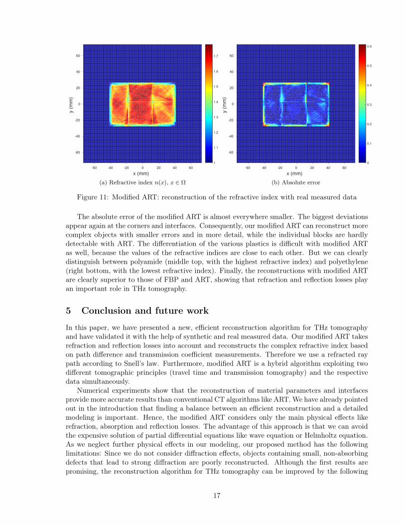
Conversely, the reconstruction with the modified ART is much better, see figure 11, andgood results can also be achieved for more complex objects. The modified ART outperforms theconventional methods FBP and ART, especially around corners, regarding shape and size of therefractive index. This is also evident from the comparison of the three methods regarding theabsolute error (see respective figures on the right-hand side).

16

x (mm)

-60 -40 -20 0 20 40 60

y (

mm

)

-60

-40

-20

0

20

40

60

1

1.1

1.2

1.3

1.4

1.5

1.6

1.7

(a) Refractive index n(x), x ∈ Ω

x (mm)

-60 -40 -20 0 20 40 60

y (

mm

)

-60

-40

-20

0

20

40

60

0

0.1

0.2

0.3

0.4

0.5

0.6

(b) Absolute error

Figure 11: Modified ART: reconstruction of the refractive index with real measured data

The absolute error of the modified ART is almost everywhere smaller. The biggest deviationsappear again at the corners and interfaces. Consequently, our modified ART can reconstruct morecomplex objects with smaller errors and in more detail, while the individual blocks are hardlydetectable with ART. The differentiation of the various plastics is difficult with modified ARTas well, because the values of the refractive indices are close to each other. But we can clearlydistinguish between polyamide (middle top, with the highest refractive index) and polyethylene(right bottom, with the lowest refractive index). Finally, the reconstructions with modified ARTare clearly superior to those of FBP and ART, showing that refraction and reflection losses playan important role in THz tomography.

5 Conclusion and future work

In this paper, we have presented a new, efficient reconstruction algorithm for THz tomographyand have validated it with the help of synthetic and real measured data. Our modified ART takesrefraction and reflection losses into account and reconstructs the complex refractive index basedon path difference and transmission coefficient measurements. Therefore we use a refracted raypath according to Snell’s law. Furthermore, modified ART is a hybrid algorithm exploiting twodifferent tomographic principles (travel time and transmission tomography) and the respectivedata simultaneously.

Numerical experiments show that the reconstruction of material parameters and interfacesprovide more accurate results than conventional CT algorithms like ART.We have already pointedout in the introduction that finding a balance between an efficient reconstruction and a detailedmodeling is important. Hence, the modified ART considers only the main physical effects likerefraction, absorption and reflection losses. The advantage of this approach is that we can avoidthe expensive solution of partial differential equations like wave equation or Helmholtz equation.As we neglect further physical effects in our modeling, our proposed method has the followinglimitations: Since we do not consider diffraction effects, objects containing small, non-absorbingdefects that lead to strong diffraction are poorly reconstructed. Although the first results arepromising, the reconstruction algorithm for THz tomography can be improved by the following

17

approach: An important property of THz radiation is the propagation according to Gaussianoptics. At this point, we neglect this physical property, suggesting the consideration of theGaussian beam profile as a promising next step. Taking into account the Gaussian beam profile,we might also consider cases in which only a part of the transmitted beam hits the receiver andthus improve the reconstruction of the absorption coefficient.

To reduce the time required for reconstruction by parallelization, using the simultaneousalgebraic reconstruction technique (SART, [5]) or more general block algebraic iterative methods(see e. g. [33]) is conceivable. Since the modifications to conventional ART concern only thematrix A and the data gabs, the iteration of e. g. SART is directly applicable, too.

Acknowledgments

This project was funded by The German Federation of Industrial Research Associations (AiF)under 457 ZN which is gratefully acknowledged by the authors.

References

[1] A. H. Andersen, Tomography transform and inverse in geometrical optics, J. Opt. Soc.Am. A, 4 (1987), pp. 1385–1395.

[2] , A ray tracing approach to restoration and resolution enhancement in experimentalultrasound tomography, Ultrasonic Imaging, 12 (1990), pp. 268–291.

[3] , Ray tracing for reconstructive tomography in the presence of object discontinuity bound-aries: A comparative analysis of recursive schemes, J. Acoust. Soc. Am., 89 (1991), pp. 574–582.

[4] A. H. Andersen and A. C. Kak, Digital ray tracing in two dimensional refractive fields,J. Acoust. Soc. Am., 72 (1982), pp. 1593–1606.

[5] , Simultaneous algebraic reconstruction technique (SART): A superior implementationof the ART algorithm, Ultrasonic Imaging, 6 (1984), pp. 81–94.

[6] M. Born and E. Wolf, Principles of optics: electromagnetic theory of propagation, inter-ference and diffraction of light, Pergamon Press, 4 ed., 1970.

[7] A. Brahm, M. Kunz, S. Riehemann, G. Notni, and A. Tünnermann, Volumet-ric spectral analysis of materials using terahertz-tomography techniques, Applied Physics B:Lasers and Optics, 100 (2010), pp. 151–158.

[8] A. Brahm, A. Wilms, M. Tymoshchuk, C. Grossmann, G. Notni, and A. Tünner-mann, Optical effects at projection measurements for terahertz tomography, Optics & LaserTechnology, 62 (2014), pp. 49–57.

[9] D. Colton, J. Coyle, and P. Monk, Recent developments in inverse acoustic scatteringtheory, SIAM Review, 42 (2000), pp. 369–414.

[10] D. Colton and R. Kress, Inverse Acoustic and Electromagnetic Scattering Theory, Ap-plied mathematical sciences, Springer New York, 3 ed., 2013.

[11] M. Defrise and C. De Mol, A note on stopping rules for iterative regularization methodsand filtered SVD, Inverse Problems: An Interdisciplinary Study, P.C. Sabatier, ed., AcademicPress, New York, (1987), pp. 261–268.

18

[12] F. Denis, O. Basset, and G. Gimenez, Ultrasonic transmission tomography in refract-ing media: reduction of refraction artifacts by curved-ray techniques, IEEE Transactions onMedical Imaging, 14 (1995), pp. 173–188.

[13] B. Ewers, A. Kupsch, A. Lange, B. Müller, A. Hoehl, R. Müller, and G. Ulm,Terahertz spectral computed tomography, in IRMMW-THz 2009. 34th International Confer-ence on Infrared, Millimeter, and Terahertz Waves, Sept 2009, pp. 1–2.

[14] B. Ferguson, Three Dimensional T-ray Inspection Systems, PhD thesis, University of Ade-laide, 2004.

[15] B. Ferguson, S. Wang, D. Gray, D. Abbot, and X.-C. Zhang, T-ray computedtomography, Optics Letters, 27 (2002), pp. 1312–1314.

[16] R. Gordon, R. Bender, and G. T. Herman, Algebraic reconstruction techniques (ART)for three-dimensional electron microscopy and X-ray photography, Journal of TheoreticalBiology, 29 (1970), pp. 471 – 481.

[17] J. Guillet, B. Recur, L. Frederique, B. Bousquet, L. Canioni, I. Manek-Hönninger, P. Desbarats, and P. Mounaix, Review of terahertz tomography tech-niques, Journal of Infrared, Millimeter, and Terahertz Waves, 35 (2014), pp. 382–411.

[18] M. Jewariya, E. Abraham, T. Kitaguchi, Y. Ohgi, M. Minami, T. Araki, andT. Yasui, Fast three-dimensional terahertz computed tomography using real-time line pro-jection of intense terahertz pulse, Opt. Express, 21 (2013), pp. 2423–2433.

[19] S. Johnson, J. Greenleaf, W. Samayoa, F. Duck, and J. Sjostrand, Reconstruc-tion of three-dimensional velocity fields and other parameters by acoustic ray tracing, inUltrasonics Symposium, 1975, pp. 46–51.

[20] A. Kak, Computerized tomography with X-ray, emission, and ultrasound sources, Proceed-ings of the IEEE, 67 (1979), pp. 1245–1272.

[21] N. Krumbholz, T. Hochrein, N. Vieweg, T. Hasek, K. Kretschmer, M. Bastian,M. Mikulics, and M. Koch, Monitoring polymeric compounding processes inline with THztime-domain spectroscopy, Polymer Testing, 28 (2009), pp. 30–35.

[22] J. W. Lamb, Miscellaneous data on materials for millimetre and submillimetre optics, In-ternational Journal of Infrared and Millimeter Waves, 17 (1996), pp. 1997–2034.

[23] S. Mukherjee, J. Federici, P. Lopes, and M. Cabral, Elimination of Fresnel reflec-tion boundary effects and beam steering in pulsed terahertz computed tomography, Journal ofInfrared, Millimeter, and Terahertz Waves, 34 (2013), pp. 539–555.

[24] F. Natterer, The Mathematics of Computerized Tomography, Classics in Applied Mathe-matics, John Wiley & Sons Ltd and B. G. Teubner, Stuttgart, 1986.

[25] F. Natterer and F. Wübbeling, Mathematical methods in image reconstruction, SIAMMonographs on Mathematical Modeling and Computation, (2001), pp. 1–207.

[26] K. L. Nguyen, M. L. Johns, L. Gladden, C. H. Worrall, P. Alexander, H. E.Beere, M. Pepper, D. A. Ritchie, J. Alton, S. Barbieri, and E. H. Linfield,Three-dimensional imaging with a terahertz quantum cascade laser, Opt. Express, 14 (2006),pp. 2123–2129.

19

[27] T. Pfitzenreiter and T. Schuster, Tomographic reconstruction of the curl and diver-gence of 2d vector fields taking refractions into account, SIAM Journal on Imaging Sciences,4 (2011), pp. 40–56.

[28] R. Piesiewicz, C. Jansen, S. Wietzke, D. Mittleman, M. Koch, and T. Kürner,Properties of building and plastic materials in the THz range, International Journal of In-frared and Millimeter Waves, 28 (2007), pp. 363–371.

[29] B. Recur, J. P. Guillet, I. Manek-Hönninger, J. C. Delagnes, W. Benharbone,P. Desbarats, J. P. Domenger, L. Canioni, and P. Mounaix, Propagation beamconsideration for 3d THz computed tomography, Opt. Express, 20 (2012), pp. 5817–5829.

[30] H. Schomberg, An improved approach to reconstructive ultrasound tomography, Journal ofPhysics D: Applied Physics, 11 (1978), pp. L181–L185.

[31] U. Schröder and T. Schuster, An iterative method to reconstruct the refractive indexof a medium from time-of-flight measurements, preprint, arXiv:1510.06899, (2015).

[32] A. Smith, M. Goldberg, and E. Liu, Numerical ray tracing in media involving continuousand discrete refractive boundaries, Ultrasonic Imaging, 2 (1980), pp. 291–301.

[33] H. H. B. Sørensen and P. C. Hansen, Multicore performance of block algebraic iterativereconstruction methods, SIAM Journal on Scientific Computing, 36 (2014), pp. C524–C546.

[34] S. Wang and X.-C. Zhang, Pulsed terahertz tomography, Journal of Physics D: AppliedPhysics, 37 (2004), pp. R1–R36.

20