1

3D modelling of near-surface, environmental effects on AEM data

David Beamish British Geological Survey, Keyworth, Nottingham, NG12 5GG, UK Beamish, D., 2004. 3D modelling of near-surface, environmental effects on AEM data. Journal of Applied Geophysics, 56, 263-280. doi:10.1016/j.jappgeo.2004.08.002 Corresponding author: David Beamish British Geological Survey, Keyworth, Nottingham, NG12 5GG, UK Email: D.Beamish@bgs.ac.uk. Tel: 0115 936 3432 Fax: 0115 936 3261 Keywords: Electromagnetic, airborne, frequency domain, 3D modelling, environment

2

Abstract This study considers the 3D modelling of compact, at-surface conductive bodies on frequency domain airborne electromagnetic (AEM) survey data. The context is the use of AEM data for environmental and land quality applications. The 3D structures encountered are typically conductive, of limited thickness (< 20 m) and form ‘point’ source locations carrying potential environmental risk. The scale of such bodies may generate single profile, ‘bulls-eye’ anomalies. In attempts to recover geological information, such anomalies may be considered to represent noise. In environmental AEM, the correct interpretation of such features is important. The study uses a combination of theoretical models and trial fixed wing survey data obtained in populated areas of the UK. Scale issues are discussed in terms of the volumetric footprints of the induced electric field generated by systems flown at both low and high elevation. One of the primary uses of AEM survey data lies in the assessment of conductivity maps. These are typically obtained using 1D conductivity models at individual measurement points. In order to investigate the limitations of this approach, 3D modelling of conductive structures with dimensions less than 350 x 350 m and thicknesses extending to 20 m has been carried out. A 1D half space inversion of the data obtained at each frequency is then used to assess the behaviour of the spatial information. The results demonstrate that half space conductivity values obtained over compact 3D targets generally provide only apparent conductivity results. For thin, at-surface bodies, conductivity values are biased to lower values than the true conductivity except at high frequency. The spatial perturbation to both coupling ratios and 1D conductivity models can be laterally extensive. The results from 3D modelling indicate that the use of horizontal derivatives applied to the conductivity models offers enhanced edge detection. The practical application of such derivatives to both regional and local scale survey data is presented.. The special case of a near-surface, metallic pipeline has been modelled. The problem constitutes an inductive limit (current gathering) response in which the perturbation is largely confined to the in-phase coupling ratios. The main perturbations, in data and conductivity models, are within about 40 m of each side of the pipeline. The maximum perturbation to the conductivity model is only a factor of 1.5 above background. Detailed survey data across a former compact landfill (about 100 x 100 m) are used to compare the model behaviour predicted by the 3D modelling with survey results. The survey, conducted at two separate altitudes, provides a demonstration of 3D effects on 1D survey models as a function of frequency and elevation. Although the nature of the landfill materials and their location are not known precisely, the mapping information appears realistic. Keywords: Electromagnetic, airborne, frequency domain, 3D modelling, environment

3

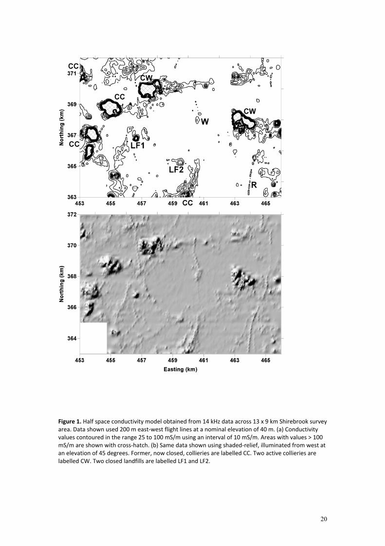
1. Introduction AEM measurements, traditionally used for reconnaissance and mineral exploration, are playing an increasing role in the assessment of land quality, environmental and hydrogeological studies. All available AEM systems, including time and frequency domain EM systems (both towed bird and fixed wing) are being applied to such studies. Large scale (regional) assessments have been undertaken (e.g. Fitterman and Deszcz-Pan, 1998; Munday et al., 2001) together with site investigation scale studies (e.g. Puranen et al., 1999; Doll et al., 2000). Here trial data obtained in the East Midlands of central England using a frequency domain fixed wing system is used to investigate AEM modelling issues in relation to environmental assessments. The majority of artificial sources of environmental impact exist at the surface (e.g. mineral loading) or may be excavated from the surface (e.g. landfills). There is then a requirement to use the survey data to define a likely source zone (e.g. the limits of a concealed former landfill) and to examine whether any migration of pollutants can be detected. Both aspects are usually assisted by the conductive nature of dissolved chemicals and their influence on increasing bulk subsurface conductivities. A background framework in environmental studies and legislation exists as the Source-Pathway-Receptor model. This model states that pollutants present in soils and sediments can potentially migrate from source to receptor(s), via different pathways. Zones of chemical concentrations, such those found in mineral stockpiles and landfills, form obvious source areas and carry potential environmental risks. Land quality issues are often most pertinent in the vicinity of populated regions and across areas with a high degree of infrastructure. Electromagnetic coupling by AEM transmitters with near-surface infrastructure is then of concern. Conceptually a near-surface zone, say 5 to 20 m in depth, and containing potential pollution sources at a variety of scales, has to be considered for environmental assessments. Pathways from the sources can, of course, extend to much greater depths. The modelling study presented here considers only simple, at and near-surface conductive bodies of limited thickness. Figure 1 shows AEM results from a 13 x 9 km trial survey flown by a frequency domain fixed wing system (Poikonen, et al., 1998) in the East Midlands of England. Flight lines are directed E-W using a 200 m (regional scale) line spacing at a nominal elevation of 40 m. Figure 1a shows the half space conductivity model obtained at a frequency of 14 kHz. The geology of the area is highly uniform and typically comprises a thick (> 80 m) Triassic sandstone unit (the Sherwood Sandstone). The background conductivity of this unit is less than 15 mS/m. The model is selectively contoured in the interval from 20 to 100 mS/m. Areas with conductivities greater than 100 mS/m are shown in cross-hatch. The area contains a series of active and closed collieries labelled CC (closed) and CW (working). The conductivity results identify the processed mineral waste (spoil) areas associated with each colliery as zones of high conductivity. The stored minerals typically possess conductivities that are > 5 above background and the storage areas (usually mine perimeters) are clearly defined by high spatial gradients in the conductivity model. Away from the immediate vicinity of the mine boundaries, a variety of anomalies are observed in the conductivity interval from 20 to 100 mS/m. A number of larger scale,

4

continuous features appear to be associated with the mine zones. Other, more localised features, occur in association with landfills (LF1 and LF2), water extraction boreholes (W) and roads (R). As discussed later, low amplitude, high wavenumber features of the conductivity model can be examined using horizontal derivatives. Figure 1b shows a shaded-relief view, illuminated from the west, of the conductivity model of Figure 1a. The image reveals a far greater number of quasi-continuous, small amplitude influences on the AEM data and the models obtained from them. Apart from the road (R), the majority of continuous features appear to be associated with subsurface infrastructure such as major water main pipe routes and underground electricity cables (11 keV). It is worth noting that the amplitude of such features (in both perturbation to coupling ratios and the conductivity model) is relatively small. The observed coupling ratios have been converted to half space conductivities in Figure 1a using a standard one dimensional (1D) inversion procedure (Beamish, 2002). One dimensional inversion of acquired data, whether half space or multilayer, is the main interpretation tool of AEM surveying. As indicated in Figure 1, a high degree of environmental (non-geological) information is introduced by three dimensional (3D) structure at various scales. When undertaking regional scale AEM surveying, as implied by a flight line separation of 200 m, many high wavenumber features (and hence 3D responses) will be of high significance when the purpose of the survey is an environmental assessment. It is worth pointing out that if the purpose of the survey was deemed to be a geological assessment, then it would be necessary to either isolate the environmental responses (e.g. as shown in Figure 1) or to attempt a ‘deculturing’ of the data as is often performed in magnetic surveys. In both cases it is necessary to understand the influence of near-surface bodies on the response characteristics and any degradation in the validity of the models that are obtained. The influence of three dimensional structure on standard 1D assessments of frequency domain AEM data has previously been discussed by Sengpiel and Siemon (1998). The limitations of 1D AEM inversion in relation to 2D overburden structure is discussed by Xie et al. (1998). Studies by Ellis (1998), Raiche (2001), Sasaki (2001) and Zhang (2003) consider forward 3D modelling and inversion of frequency domain AEM data. The nature of the data shown in Figure 1 defines a requirement to understand AEM response and model characteristics from a variety of environmental sources. The sources may be classified along the following lines. The targets are typically at and near-surface and are relatively conductive. Some of the environmental targets may be highly conductive in relation to the host geology. They are typically two and three dimensional at a variety of scales. At one limit the lateral scale will be substantially greater than the AEM footprint while other features (e.g. infrastructure) will appear as quasi-linear conductive contrasts with dimensions much smaller than the footprint scale. Between these two limits, a set of features exist that may be of the same order as the footprint scale. The main emphasis of the present study concerns the characterisation of smaller scale environmental anomalies that would be detected as part of larger scale AEM surveys. There is a distinction between this form of general surveying and localised site specific environmental AEM surveys that have been conducted across potentially hazardous areas (e.g. Doll et al., 2000; Beamish and Mattsson, 2003).

5

The most common method used for the interpretation of AEM data is that of 1D inversion. The source is three dimensional and the model is assumed to be one dimensional. When considering 3D modelling, the scale of the 3D body in relation to that of the source field is important. Following a description of the AEM survey data used here, scale issues are first considered using a volumetric assessment of AEM footprints. Footprint scales in AEM vary with source polarisation and with elevation. Here both Vertical Magnetic Dipole (VMD) and Horizontal Magnetic Dipole (HMD) sources are considered for elevations of 40 m and 90 m. The need to consider both high and low level surveying in populated areas, due to regulatory restrictions, has been discussed by Lee et al. (2001). Forward 3D frequency domain modelling of AEM data has previously been considered for a few specific cases. Generally the studies relate to the influence of concealed subsurface bodies. Here only at-surface, generic environmental source bodies are considered. This type of body has a strong influence on all the frequencies used in AEM surveying since the sensitivity functions are a maximum at the surface (McGillivray et al.,1994; Tølbøll and Christensen, 2002). The 3D forward modelling code developed for AEM data by Sasaki (2001) is used. The lateral scale of the single prism bodies considered ranges from 320 x 320 m to 20 x 20 m. Thicknesses of the conductive bodies range from 5 m to 20 m. The special case of a simulated pipeline is also considered. The frequencies used in the modelling range from 512 Hz to 128 kHz while special emphasis is given to the two frequencies (3 and 14 kHz) associated with an existing fixed wing system. Only single profiles of data collected across the central section of each model are presented in order to identify the nature of the near-surface 3D effects. The results obtained (the coupling ratios) are used in a single frequency, half space inversion. This form of model is common in AEM interpretations and is used to further assess the influence of the 3D body on the data from each of the frequencies. Both VMD and HMD coplanar systems are considered. Using the results from the 3D modelling it is demonstrated that the use of horizontal spatial gradients applied to a profile of 1D conductivity models offers enhanced edge detection. Finally, in order to illustrate the response behaviour predicted by the modelling results, trial survey results across a small legacy landfill (100 x 100 m) are presented. The area containing the former landfill was flown using 50 m flight lines. Two surveys were conducted at 40 m and 90 m. The results provide a demonstration of 3D effects on compact 1D conductivity distributions as a function of frequency and elevation. 2. AEM survey data Frequency domain AEM data is acquired using either fixed wing (wing tip sensors) or helicopter (towed bird HEM) systems. The data comprise in-phase (P) and in-quadrature (Q) components (coupling ratios in ppm) at each operational frequency. Coupling ratios are here defined as the secondary to primary field ratio, multiplied by 106, for both P and Q components. Fixed wing systems such as the Twin Otter operated by the Geological Survey of Finland (GTK) can be successfully operated at elevations greater than 90 m. This makes such a system attractive where air-space is

6

highly regulated and conditional approval includes restrictions on the minimum survey altitude (usually a function of population density). The GTK system is described by Poikonen, et al. (1998). At present the fixed wing system is limited to two operational frequencies (3 and 14 kHz) using two pairs of vertical coplanar coils. These form an HMD coplanar system with a coil separation of 21.4 m. HEM towed bird systems provide a set of distributed frequencies (say 5) with typical limits from several hundred hertz to over 100 kHz. Signal to noise issues usually restrict the bird (sensor) elevation to the range 30 to 40 m above ground. Although a variety of coil pair configurations have been utilised (Fraser, 1978), we restrict our attention here to coplanar coil pairs forming HMD and VMD systems. The flight line spacing used for a survey depends on the survey objectives and is a cost consideration. According to Beamish (2003), effective survey design in AEM can be understood in relation to the scale of the footprint. Sampling of data along the flight line direction is typically less than 15 m so that successive footprints overlap and form a moving-average measurement along the flight line. Flight line spacing can be designed to achieve footprint overlap across lines, thus achieving high resolution. Larger line spacings result in isolated across line footprints. The scale of an AEM footprint is primarily dependent on survey altitude and the sensor orientation (e.g HMD or VMD). For high level (say 90 m) surveying both HMD and VMD systems typically provide cross line footprint overlap for flight line spacings of 200 m and less. For lower level surveying, consideration should be given to flight line spacings of 100 m, or less, depending on the system considered (Beamish, 2003). These issues are important when considering the small lateral dimensions of many isolated environmental targets. Figure 2 shows a 1 x 1 km area taken from the trial survey discussed previously. The measurement points are shown by cross symbols. The area contains a former landfill that operated between 1930 and 1976 (estimated) and occupied a former quarry. Details (e.g. mapped information) of the quarry and landfill are scant. The site occupies a zone in the northern centre of the map. The AEM survey data have been inverted to form a half space conductivity model for each frequency (described later). Figure 2 shows the contoured values of the 3 kHz conductivity model with a lower limit of 20 mS/m that clearly defines a ‘bulls-eye’ anomaly, largely confined to one survey line. The higher frequency (14 kHz) half space model displays a similar anomaly pattern to that shown. This behaviour is typical of at and near-surface influences on AEM data, in that, data at all frequencies are perturbed. The anomaly is compact on a scale of several hundred metres in both N-S and E-W directions. Very rapid spatial gradients are observed across the zone indicating its three dimensional nature. The modelling of such isolated conductive 3D features is considered following an assessment of footprint scale issues. 3. Scale issues in 3D AEM modelling A consideration of the electromagnetic interaction of a 3D dipolar source with a 3D Earth is not simple. In order to establish simple rules it is necessary to first consider single bodies, in a uniform or layered half space. In order to understand general behaviour, knowledge of the size of the system footprint in relation to the size of the body is important (Kovacs et al., 1995; Xie et al., 1998). Following the work of Liu

7

and Becker (1990), Beamish (2003) studied AEM footprints in terms of at-surface electromagnetic skin distances for finitely conducting half spaces. In order to remove system specific parameters, the revised footprints were calculated for the limiting cases of vertical and horizontal dipolar transmitter excitation. The footprint/altitude ratio was found to have a primary dependence on altitude and a secondary dependence on conductivity and frequency. Footprints due to an HMD transmitter were smaller, by a factor of between 1.3 and 1.5, than those due to a VMD operated at the same height. It was pointed out by Beamish (2003) that dipolar footprints in finitely conducting media are volumetric. An attenuation scale length in the vertical direction (a skin depth) occurs in association with the at-surface footprint. Beamish (2004) studied the vertical decay scale lengths, using the at-surface position of maximum electric field. The method follows the equivalent skin depth definition used in the plane-wave case. In the plane-wave case, skin depth is defined at the depth at which the induced electric field has decayed to 1/e of its surface value. The surface is also the location of maximum induced field. For elevated dipoles it is necessary to first define the geometry of the surface (maximum) field and then to calculate the subsurface decay, again using a 1/e criterion, of the geometrical field. The calculation must be done numerically. The revised definition enabled the same skin depth estimate to be obtained for both cases of vertical and horizontal dipolar excitation. Dipolar skin depths are found to be much smaller than their plane wave counterparts except at high frequency (> 50 kHz) and in combination with high conductivity. For the majority of airborne systems the influence of altitude on skin depth is highly significant. Dipolar skin depths increase with increasing sensor elevation. Low frequencies display the greatest sensitivity. At low elevation (< 40 m), geometrical attenuation dominates the behaviour of the skin depth. The above volumetric assessments of the induced current distribution due to dipolar excitation need to be considered in relation to 3D modelling. The lateral scale of the at-surface bodies considered later is less than 350 m and thicknesses range from 5 to 20 m. In order to illustrate the issues, typical transmitter skin volumes (e.g. Beamish, 2004) in a homogenous medium with a conductivity 10 mS/m and for an intermediate AEM frequency of 10 kHz have been calculated. Here the volume in which the modulus of the total induced electric field has decayed to 1/e of the maximum electric field (located on the surface of the half space) is shown across a volume of 300 x 300 x 30 m. Figure 3 shows the skin volume for a VMD source (Fig. 3a) and for an HMD source (polarised in the x-direction, Fig. 3b). In both cases the transmitters are 40 m above the origin. The SE quadrant of the region has been made transparent in order to view the interior and a x 4 degree of vertical exaggeration has been applied. Opaque depth slices are shown at depths of 5 and 15 m (corresponding to two of the thicknesses of the bodies studied). The at-surface scale of a 100 x 100 m body is also indicated. For a transmitter elevation of 40 m, lateral skin footprints for both VMD and HMD sources, are considerably less than the 300 x 300 m scale shown. At the 100 x 100 m scale, lateral skin footprints either fully (in the case of the VMD) or partially (in the case of the HMD) exceed the surface dimensions shown. For lateral scales of 50 m and less, both sets of footprints would exceed the scale of the structure. Vertical dipolar skin depths are about 21 m in both cases.

8

The calculation has been repeated with identical parameters apart from an increase in transmitter elevation to 90 m. Figure 4 shows the skin volumes obtained. For a VMD transmitter (Fig. 4a), the lateral skin footprint just exceeds the 300 x 300 m scale, while the more compact footprint of the HMD source (Fig. 4b) is well contained within the boundary. At the 100 x 100 m scale indicated, both VMD and HMD footprints exceed the surface area indicated and, obviously, continue to exceed the dimensions of smaller scale structures. At an elevation of 90 m, vertical dipolar skin depths exceed the depth extent of 30 m shown. Although the calculations have only been presented for a mid-range frequency of 10 kHz, and a half space of 10 mS/m, the results have a general significance (e.g. Beamish, 2004). From the results it is apparent that transmitter orientation and elevation will influence the interaction of the induced current system with at-surface, environmental targets whose dimensions are, say, less than 300 x 300 m. Lower level surveys (e.g. 40 m) provide a greater focus (in terms of the lateral scale of the induced current distribution) of smaller scale features than higher level surveys. The use of HMD sources accentuates the focusing. In terms of vertical dipolar skin depths, even low level sources exceed the vertical dimensions of many at-surface features of interest. It should be noted that the environmental (geochemical) products that may originate in such zones may, however, require assessment over larger lateral distances and deeper vertical scales than those considered above. 4. 3D modelling Initial AEM modelling procedures involving algorithms for thin-plate structures in free-space and in layered hosts have been supplemented by more general 3D numerical procedures. The two main approaches to 3D frequency domain modelling involve either differential or integral equation methods (Hohmann, 1988). Forward 3D frequency domain AEM modelling of subsurface features has only been conducted in a few cases. Typically, simple buried prisms have been considered (e.g. Ellis, 1998; Sengpiel and Siemon, 1998; Sasaki, 2001). At-surface conductivity contrasts, to which AEM data are most sensitive, appear to only have been studied in a few cases (e.g. Raiche, 2001). Here, a differential equation approach developed by Sasaki (2001) for the forward modelling component of a 3D inversion scheme has been used. The single body models considered here are formed using rectangular cells on a staggered grid of 53 x 53 x 42 (117,978 blocks). Cell dimensions were adjusted in accord with the scale of the model considered. The smallest cell dimension used was 0.1 m. The homogenous background half space is taken to be 10 mS/m. The models are constructed to be symmetrical about the vertical axis and only a one-sided profile (in the x direction) though the centre of the body is considered. The data modelled comprise the in-phase (P) and in-quadrature (Q) coupling ratios between coplanar VMD and HMD systems. The magnitude of the coupling ratios depends on the separation between transmitter and receiver (it is proportional to the cube of the separation) and is different for the two orientations considered. Here a typical fixed wing separation of 20 m is used for modelling. The interpretation of AEM data typically proceeds using one dimensional (1D) conductivity models. Common

9

procedures largely developed and described by Fraser (1978, 1986) comprise the modelling of the observed coupling ratios by a pseudo-layer algorithm. A separate half space model is determined at each frequency. It is also possible to perform iterative least-squares inversion of AEM data (Paterson and Redford, 1986; Sengpiel and Siemon, 1998) to obtain an equivalent half space model. These procedures also provide a misfit that aids discrimination of invalid data (i.e. non 1D and/or layered influences). Here the inversion described by Beamish (2002) is used on the modelling results. For the small numbers of observations used in the inversion (i.e. 2), an L1 norm (based on the sum of differences) rather than an L2 norm (based on the sum of squared differences) misfit parameter has proved useful. Here the L1 norm percentage error is defined as: n

L1(%) = 100.0 Σ │ Oi – Ci │ / Ci …(1) i=1

where Oi is the i’th observation (an in-phase or in-quadrature coupling ratio) and Ci is the corresponding calculated value. The coupling ratios (P and Q) obtained across a single conducting body with dimensions of 320 x 320 x 20 m are shown in Figure 5. The results shown are for an HMD source (x-directed) at a height of 40 m. The P (solid symbols) and Q (open symbols) ratios are shown at three widely spaced frequencies from 512 Hz to 128 kHz. The position of the edge of the body is indicated by a dash line and a logarithmic scale is used. Coupling ratios at all 3 frequencies are perturbed to high values, in at least one of the components, by the conductive body. For an HMD source at an elevation of 40 m, the footprint is contained within the at-surface dimensions of the body at all frequencies. The perturbation, from background values, takes place across a relatively fixed lateral scale for the parameters used. This ‘adjustment distance’ is most clearly defined at the lowest frequency and extends over 150 m, as indicated in Figure 5. A 1D inversion of the P and Q data for each frequency produced the half space models and misfits shown in Figure 6. Over the lateral scale shown (300 m) the detection of the background half space and the correct ‘level’ for the conductivity of the body is achieved at the two highest frequencies. Allowing for some imprecision, the lateral scale of the perturbation from the background conductivity to that of the body covers about 150 m. The lowest frequency (512 Hz) is influenced by the finite thickness of the body (it is not a half space) and returns a conductivity of about 40 mS/m across a major portion of the body. The misfits (Fig. 6b) reflect the same behaviour. Although increases in misfit are observed in association with models in the vicinity of the body, the misfit levels observed at the two higher frequencies would probably not be detectable in actual survey data. In contrast, the misfits of the models obtained at the lowest frequency clearly indicate the existence of a non-uniform half space. In general, the misfit parameter associated with a 1D inversion does not always identify the existence of non-tabular structure.

10

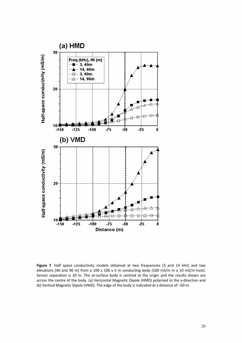
Many zones of environmental interest are contained within thin structures (e.g. < 20 m) at or near the surface. A study, similar to that above, has been conducted for a body with lateral dimensions of 100 x 100 m and thicknesses of 5 and 15 m. As discussed previously, such thicknesses are typically contained within the vertical skin depth for both low and high level AEM surveying. Since there is a considerable variation of footprint scale with elevation, two elevations (40 and 90 m) are considered. Again the sensor separation is fixed at 20 m and only 2 frequencies (3 kHz and 14 kHz) are used to examine frequency dependent effects. Both VMD and HMD coplanar systems are considered. Only the behaviour of half space inversion results obtained from single frequency data are presented. Figure 7 shows the half space inversion results obtained for a 100 x 100 x 5 m body (100 mS/m) in a 10 mS/m uniform background. Results are shown for two frequencies (3 and 14 kHz) and at two elevations (40 and 90 m), Figure 7a shows the results for an HMD coplanar system and Figure 7b shows the results for a VMD coplanar system. In contrast to the thicker body discussed previously, the true conductivity of the 5 m thick body is not observed in the results. The body influences all the conductivity models shown and would be probably be detectable as a relatively conducting zone in all the data considered. As expected, the body has a significantly greater detectability in the lower level (40 m) survey data and in the higher frequency results. The lateral extent of the body edge effects is slightly larger in the VMD results, with the HMD results displaying larger gradients (see later). For completeness, the equivalent set of results obtained when the thickness of the body increases to 15 m is shown in Figure 8. The doubling of the scale of the conductivity axis should be noted. The behaviour is very similar to that of the previous case. The overall outcome of increasing thickness is that the body becomes increasingly detectable and conductivities associated with the body are closer to the correct level even though the body constitutes a non-uniform half space. The results of Figures 7 and 8 demonstrate that half space conductivity values obtained over compact 3D targets generally provide only apparent conductivity results. For thin, at-surface bodies, conductivity values are biased to lower values than the true conductivity except when high frequencies are used. The variation of values and spatial gradients observed with frequency and/or survey altitude results from the three dimensional nature of the structure. Similar analyses of 3D bodies with decreasing lateral dimensions have been conducted. Detection, meaning the perturbation to the coupling ratios and subsequent conductive signature in half space inversion of the data, is best maintained in the high frequency data and in the HMD response. By a reduced lateral scale of 20 x 20 m, the influence of the body becomes insignificant in the VMD response (thicknesses of 5 and 15 m), while a significant response (a perturbation in the coupling ratios > 100 ppm) is observed in the HMD response for both thicknesses at 14 kHz. The results refer to the lower level survey altitude of 40 m. 4.1 Horizontal derivatives The horizontal spatial gradients, referred to above, form a further, enhanced method of detection. Gradients of magnetic and gravity data are routinely used to enhance the edges of anomalies, or as input to interpretation techniques such as analytic signal

11

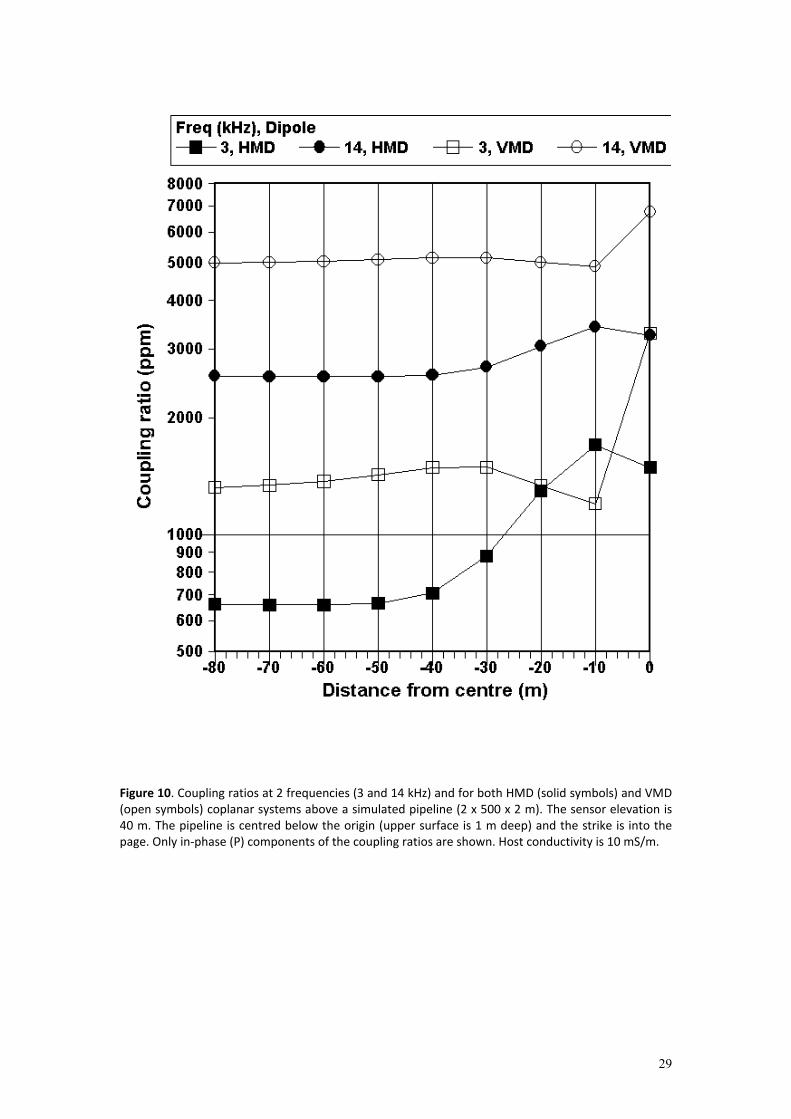
analysis or Euler deconvolution. Both vertical and horizontal derivatives and combinations of them are used to better delineate body edges (Blakely, 1995). Sunshading is another commonly used technique for emphasising features in an image that have a specific orientation. The procedure that forms the reflectance image involves the use of two orthogonal horizontal gradients (Horn, 1982). Edge detection, involving the use of horizontal derivatives, requires good quality data. The 1D conductivity models, obtained from the 3D modelling results, have first been resampled to a higher density using cubic spline interpolation. Figure 9 shows the horizontal derivative for the high frequency (14 kHz) data for both thin (5 m) and thick (15 m) 3D models. As expected, the HMD source provides a more compact and larger derivative response than the VMD source. The peak value is located just outside (10 to 20 m away from) the edge of the body. Lower sensor elevations provide the largest derivative response. When symmetry across the body is considered it should be appreciated that the negative edge derivative response shown (at negative distances) will be followed by an equivalent positive derivative response (at positive distances). In essence, the horizontal derivative has a ‘dipolar’ form approximately outlining the edges of the body. The regional scale use of a sunshading algorithm, applied to 14 kHz conductivity models was shown previously in Figure 1b. A further example of the use of horizontal gradients applied to detailed high resolution survey data is given later. 4.2 Pipeline effects Significant AEM responses are generated by coupling with infrastructure in the form of pipelines and, possibly, major cable routes. A distinction should be made between active, large voltage sources such as overhead (pylon) routes that radiate a competing EM field and passive, metallic conductors. The 3D modelling was extended to the case of a metallic pipeline using a body of 2 x 500 x 2 m with a conductivity of 109 mS/m embedded in a uniform host of 10 mS/m. The cross-section of 2 x 2 m was used for grid modelling convenience; the intention is to provide a cross-sectionally compact, elongate conductive feature in relation to the scale of the footprint. The skin-effect within such a highly conductive body should remove the requirement to model the pipe as a hollow body. The conductive body was inserted below 1 m of cover and thus extends from 1 to 3 m below the surface. A survey profile normal to and through the centre of the body is considered here. The sensor altitude is 40 m with the HMD source polarised normal to the strike of the simulated pipe. The problem constitutes an inductive limit (current gathering) response in which the perturbation, due to the body, is largely confined to the in-phase (P) coupling ratios. The coupling ratios obtained for an HMD coplanar system (solid symbols) and a VMD coplanar system (open symbols) at frequencies of 3 and 14 kHz are shown in Figure 10. Only the P component responses are shown and a logarithmic scale is used. The main perturbations are now quite localised, being within about 40 m of the body. The largest perturbations are generated in the lower frequency (3 kHz) responses. The HMD response, when symmetry across the body is considered, forms a classical ‘M’ signature peaking, in this case, some 10 m away from body. The amplitude scale of the perturbations is very similar for both HMD and VMD systems. At 3 kHz the coupling ratio amplitude increases by a factor of about 2.5 above background; this

12

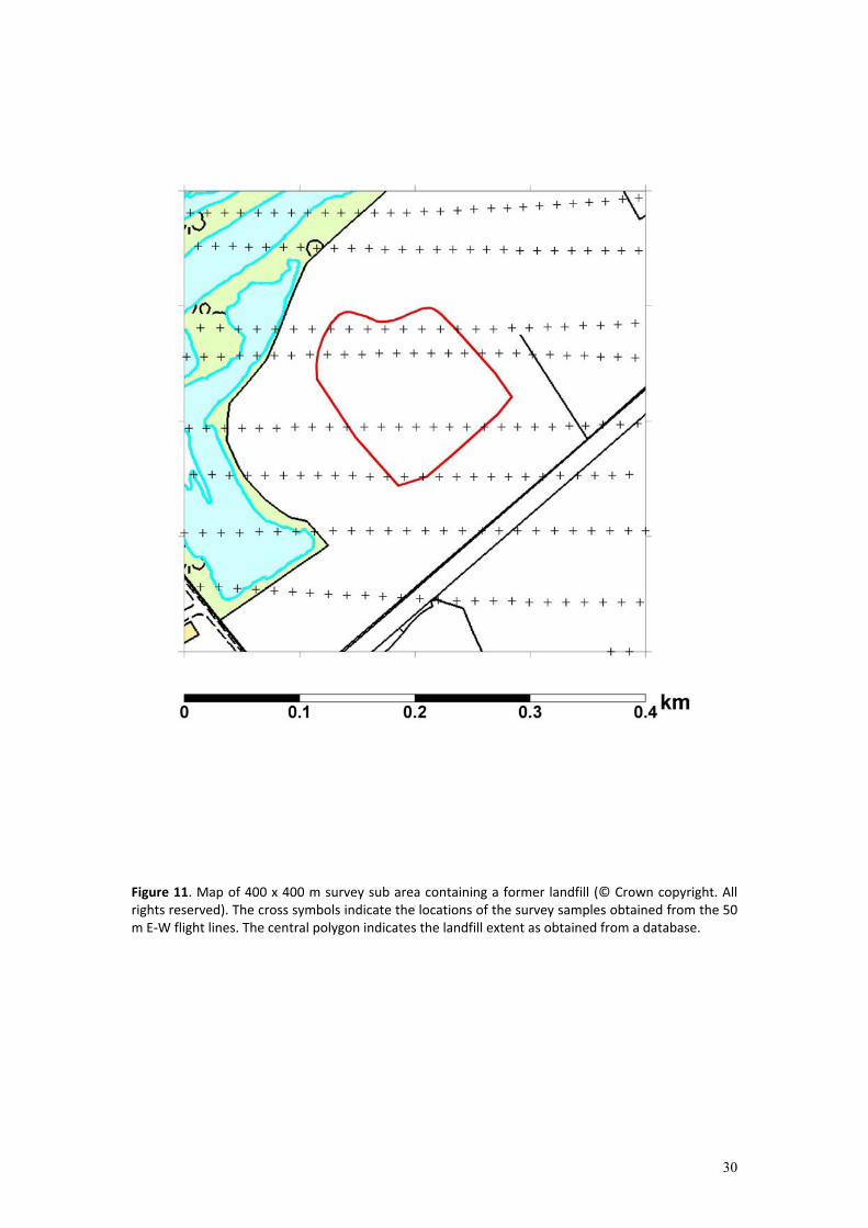
factor is reduced to about 1.3 at the higher frequency of 14 kHz. When these data are inverted to provide half space conductivity models only small perturbations are observed. Peak values of the conductivities associated with the pipeline are largely independent of frequency being 15 and 13 mS/m for the HMD source at 3 and 14 kHz, respectively. The conductivities for the VMD source are very similar being 16 and 13 mS/m, respectively. Modelling of the same systems when flown parallel to the pipeline indicates that the same amplitudes and anomaly shapes are maintained As observed in Figure 1, the magnitude of the majority of pipeline effects (assumed) are of second order to the environmental effects and are best observed, and identified, using a display of the horizontal derivatives. 5. A 3D field example In order to illustrate the detection and characterisation of a 3D environmental target by an AEM survey, data obtained across a small scale legacy landfill is considered. The example is taken from a 4 x 1.5 km trial area flown by the Twin-Otter system. In contrast to the sandstone geology of the area shown in Figure 1, this smaller area contains a series of clay rich limestones that provide a highly conductive host. The sub area chosen is only 400 x 400 m and it contains a former landfill of about 100 x 100 m. The landfill, occupying a former quarry, operated for about 18 years between 1953 and 1971 and is capped by permeable soils. The AEM survey was conducted some 28 years after closure. The site was licensed for household and industrial waste and is known to have accepted farm effluent at the rate of about 5000 gallons a week. A map of the 400 x 400 m area is shown in Figure 11. An outline of the polygon of the former quarry site is located in the centre of the area. The information would probably have been digitised from paper records. It is stressed that the polygon may not be wholly accurate with regard to the position of the quarry/landfill. Other instances from the survey data indicate that geophysical results may provide greater spatial accuracy than database records. The polygon is primarily used here for a spatial reference. The survey was conducted using E-W flight lines 50 m apart. In the absence of such high resolution sampling, small scale features such as the landfill considered here would, at best, be detected along only one flight line (e.g. Figure 2). The flight line sampling shown in Figure 11 indicates that the landfill area is traversed by about 4 flight lines. The flight lines shown in Figure 11 (cross symbols) relate to a survey conducted at a nominal elevation of 40 m. A second survey was flown at an elevation of 90 m, again using flight lines 50 m apart, as part of a technical evaluation. The two surveys, at considerably different altitudes, together with the lateral scale of the target, constitute approximations to the footprint scale issues discussed previously and the 3D modelling results obtained above. Again it is simplest to describe the data characteristics in terms of the best fitting, half space conductivity models at each of the two frequencies. Figure 12a shows selected contours of the half space conductivity models obtained for the 3 kHz data (contours without infill) and for the 14 kHz data (contours with infill). The data come from the 40 m elevation survey. The lowest conductivity value contoured in each of the two cases isolates the high conductivity anomaly associated with the landfill site. The

13

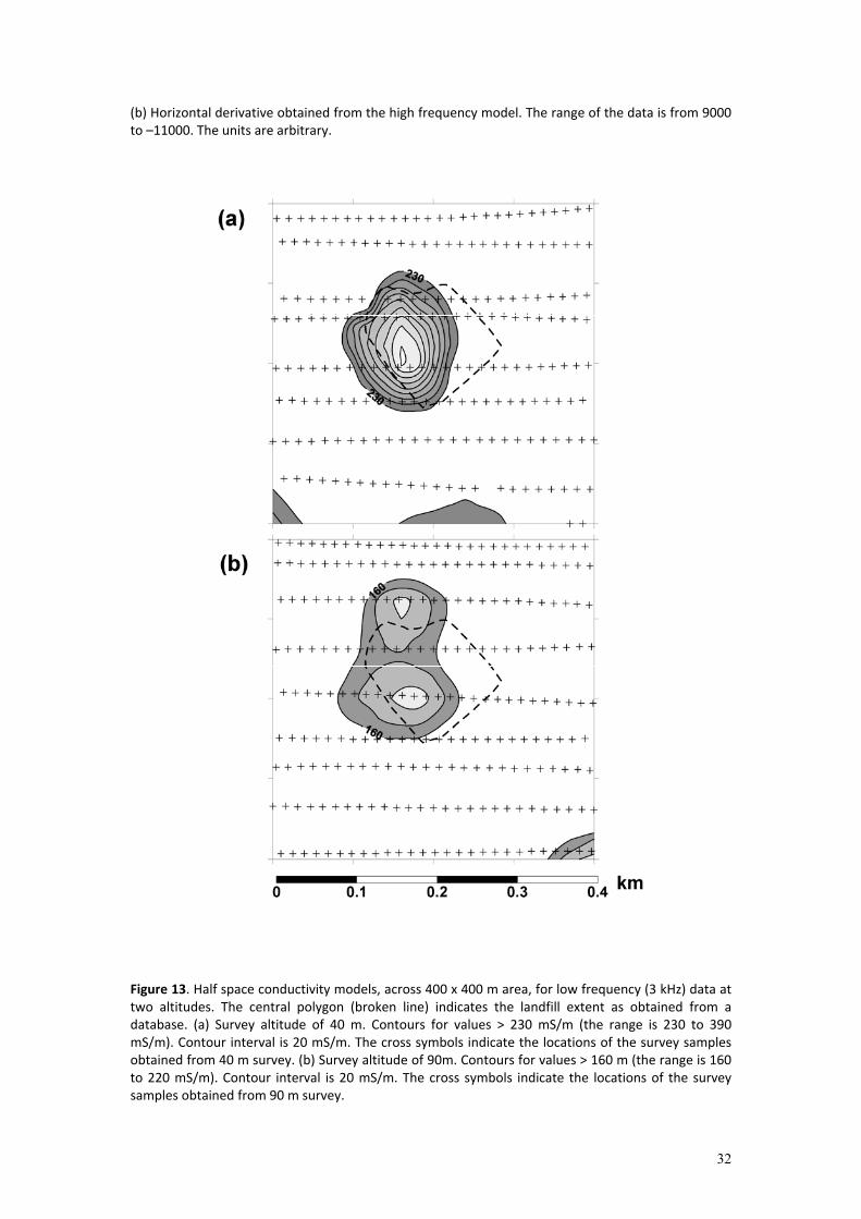
lower frequency results show contours between 225 and 400 mS/m while the higher frequency results show contours between 400 and 1000 mS/m. The same contour interval of 50 mS/m is used in each case. Clearly the higher frequency model displays much larger conductivity values and spatial gradients than that of the lower frequency model. The half space conductivities obtained can be compared with the 3D HMD modelling results at an elevation of 40 m in Figure 7a (model thickness of 5 m) and Figure 8a (model thickness of 15 m). The results from both of these models indicate significant increases in the amplitude and spatial gradients of the higher frequency model over the conductive body. There is a displacement between the maxima of the two models shown in Figure 12 and this is likely to be genuine given the flight line spacing shown. As indicated by the 3D modelling results, the edges of the conductive zones establish conductivity gradients beyond and within the conductive zone. The use of horizontal derivatives to aid edge detection was discussed in relation to the results of the 3D modelling. For the at-surface models considered, the higher frequency data provide the greatest discrimination. Here the 14 kHz conductivity models are used. The high frequency models along individual flight lines were first subjected to cubic spline interpolation to provide a level of smoothing and resampling. The first horizontal derivative of these data was then formed. Figure 12b shows the contoured results with a peak set of positive values (1000 to 9000) formed to the west of a slightly larger set of negative values (-1000 to –11000). A zero level, along an approximately N-S axis, defines an ‘anomaly centre’. Obviously the N-S extent of the information is limited by the flight line sampling. A more precise representation is obtained along the E-W flight line direction. Despite the sampling limitations, a well-defined zone of maxima and minima outlines a conductive feature that is approximately 100 x 100 m. Given the spatial behaviour of the horizontal derivative model results (Fig. 9), it is likely that the subsurface conductivities contributing to the 14 kHz data are contained within the reference polygon shown. The lower frequency (3 kHz) half space conductivity models obtained by two surveys at elevations of 40 and 90 m are shown in Figure 13. In this comparison, the difference in flight line behaviour of the two surveys is critical. The cross symbols denote flight line observations for the 40 m survey in Figure 13a and for the 90 m survey in Figure 13b. Figure 13a (40 m elevation) shows the contoured conductivity with a lower cut-off of 230 mS/m. This conductivity level isolates the landfill response from background (lower values). The range of the data is 230 to 390 mS/m. Figure 13b (90 m elevation) shows the contoured conductivity with a lower cut-off of 160 mS/m using the same contour interval of 20 mS/m. This level again isolates the landfill response from background (lower values). The range of the data is from 160 to 220 mS/m. The behaviour follows that predicted by the modelling experiments. The values obtained at the higher elevation (160 to 230 mS/m) indicate a separate range to those obtained at the lower elevation (230 to 390 mS/m) at the same frequency. These ranges are both significantly lower than the range of 400 to 1000 mS/m observed at the higher frequency at an elevation of 40 m (Fig. 12). In fact, in the case of compact 3D models all the half space conductivity values are, necessarily, incorrect and biased to low values as shown in the modelling results of Figures 7 and 8. Acknowledging the fact that the two models shown in Figure 13 provide only

14

apparent conductivity values, the spatial definition of this small landfill from both surveys is similar. Where definition is high, along the flight line direction, a similar E-W lateral extent is observed. As discussed previously, definition perpendicular to the flight line direction is critically dependent on flight line spacing, and this is largely responsible for the variation in model behaviour to the north of the reference landfill polygon. 6. Conclusions This study has considered the 3D modelling of compact, at-surface conductive bodies on frequency domain AEM data. These types of responses have relevance to the use of AEM for environmental and land quality applications. One of the primary uses of AEM data lies in the mapping information provided by conductivity models. The mainstay of this mapping information is provided by 1D models obtained at individual measurement points. The limitations of this approach are that the zones of interest are typically three dimensional. Only half space conductivity models have been considered in the inversion of field data . It should be appreciated that these models are a limiting, but still useful, case of multilayer 1D assessments. AEM surveys in populated regions may give rise to a variety of survey elevations. In such areas, low nominal survey elevations cannot be routinely maintained due to regulatory requirements. The study has considered a range of flying heights of 40 and 90 m. The elevation has important consequences on the focusing of the AEM footprint (i.e. its lateral scale) in relation to the compact environmental features considered. The modelling of AEM data using 3D bodies is inevitably system specific. Both VMD and HMD coplanar systems have been considered. All systems will use a range of frequencies, typically more than two, extending from a low to a high frequency limit. At and near-surface bodies influence all AEM frequencies due to the behaviour of the sensitivity functions. 3D model results have only been considered for at-surface conductive features with thicknesses ranging from 5 to 20 m. The results demonstrate that half space conductivity values obtained over compact 3D targets generally provide only apparent conductivity results. For thin, at-surface bodies, conductivity values are biased to lower values than the true conductivity except when high frequencies are considered. The variation of model values and spatial gradients observed with frequency and/or survey altitude results from a complicated spatial interaction of the 3D induced current system and the 3D body considered. The use of horizontal derivatives obtained from 1D conductivity models has been proposed to aid in the edge detection (spatial localisation) of 2D and 3D bodies. Models obtained for the highest survey frequency are the most appropriate. The derivative response is far more localised than either the perturbation to the coupling ratios or the 1D conductivity models obtained from them. The HMD source provides a more compact and larger derivative response than the VMD source. Theoretical and survey examples have been presented. The inductive limit response provided by a 2D near-surface pipeline has also been considered. The response is largely independent of frequency and source orientation. The magnitude of the pipeline effect is of second

15

order to the environmental effects (in the studies used) and is best observed, and identified, using a display of the horizontal derivatives. A detailed (400 x 400 m) study of a compact, former landfill has been used to verify the behaviour of the modelling results obtained. The landfill, despite its age (28 years after closure), its previous use (domestic, light industrial and agricultural), its geological setting (conductive clays) and its size (approximately 100 x 100 m) still provides a highly detectable effect within a larger regional survey. The survey conducted at a 50 m flight spacing and at two separate altitudes (40 and 90 m) provides a demonstration of 3D effects on 1D conductivity models obtained from survey data as a function of frequency and elevation. Although the precise nature of the landfill materials and their location is not known, the mapping information provided by the AEM data appears realistic. Acknowledgements My special thanks go to Professor Y. Sasaki for providing the 3D AEM modelling program used in the study. My thanks also go to the two reviewers and Editor for constructive comments. This report is published with the permission of the Executive Director, British Geological Survey (NERC). References Beamish, D., 2002. A study of conventional and formal inversion methods applied to high-resolution AEM data. J. Appl. Geophys. 51, 75-96. Beamish, D., 2003. Airborne EM footprints. Geophys. Prosp. 51, 49-60. Beamish, D. and Mattsson, A., 2003. Time-lapse airborne EM surveys across a municipal landfill. J. Environmental & Engineering Geophysics 8, 157-165. Beamish, D., 2004. Airborne EM skin depths. Geophys. Prosp. Accepted for publication. Blakely, R.J., 1995. Potential Theory in Gravity and Magnetic Applications. Cambridge University Press, 441pp. Doll, W.E., Nyquist, J.E., Beard, L.P. and Gamey, T.J. 2000. Airborne geophysical surveying for hazardous waste site characterisation on the Oak Ridge Reservation, Tennessee. Geophysics 65, 1372-1387. Ellis, R.G., 1998. Inversion of airborne electromagnetic data. Exploration Geophysics 29, 121-127. Fitterman, D.V. and Deszcz-Pan, M. 1998. Helicopter EM mapping of saltwater intrusion in Everglades National Park. Exploration Geophysics 29, 240-243.

16

Fraser, D.C., 1978. Resistivity mapping with an airborne multicoil electromagnetic system. Geophysics 43, 144-172. Fraser, D.C., 1986. Dighem resistivity techniques in airborne electromagnetic mapping. In: Palacky, G.J. (Editor.), Airborne Resistivity Mapping, Geological Survey of Canada, Paper 86-22, pp. 49-54. Hohmann, G.W., 1988. Numerical modeling for electromagnetic methods of geophysics. In: Nabighian, M. (Editor), Electromagnetic Methods in Applied Geophysics - Theory. Vol. 1. SEG, Tulsa, pp. 313-363. Horn, B.K.P., 1982. Hill shading and the reflectance map. Geoprocessing, 2, 65-146. Kovacs, A., Holladay, J.S. and Bergeron Jr., C.J. 1995. The footprint/altitude ratio for helicopter electromagnetic sounding of sea-ice thickness: Comparison of theoretical and field estimates. Geophysics 60, 374-380. Lee, M.K., Peart, R.J., Jones, D.G., Beamish, D., and Vironmaki, J., 2001. Applications and challenges for high resolution airborne surveys in populated areas. EAGE 63nd Conference, Amsterdam, Extended Abstracts, Paper IA-1. Liu, G. and Becker, A. 1990. Two-dimensional mapping of sea-ice keels with airborne electromagnetics. Geophysics 55, 239-248. McGillivray, P.R., Oldenburg, D.W., Ellis, R.G. and Habashy, T.M. 1994. Calculation of sensitivities for the frequency domain electromagnetic problem. Geophys. J. Int. 116, 1-4. Munday, T.J., Macnae, J., Bishop, J. and Sattel, D., 2001. A geological interpretation of observed electrical structures in the regolith: Lawlers, Western Australia. Exploration Geophysics 32, 36-47. Paterson, N.R., Redford, S.W., 1986. Inversion of airborne electromagnetic data for overburden mapping and groundwater exploration. In: Palacky, G.J. (Editor), Airborne Resistivity Mapping, Geological Survey of Canada, Paper 86-22, pp. 39-48. Poikonen, A., Sulkanen, K, Oksama, M., and Suppala, I. 1998. Novel dual frequency fixed wing airborne EM system of Geological Survey of Finland (GTK). Exploration Geophysics 29, 46-51. Puranen, R., Säävuori, H., Sahala, L., Suppala, I., Mäkilä, M. and Lerssi, J. 1999. Airborne electromagnetic mapping of surficial deposits in Finland. First Break, May 1999, 145-154. Raiche, A., 2001. Choosing an AEM system to look for kimberlites – a modelling study. Exploration Geophysics 32, 1-8. Sasaki, Y., 2001. Full 3-D inversion of electromagnetic data on PC. J. Appl. Geophys. 46, 45-54.

17

Sengpiel, K.-P., Siemon, B., 1998. Examples of 1-D inversion of multifrequency HEM data from 3-D resistivity distribution. Exploration Geophysics 29, 133-141.

Tølbøll R.J. and Christensen, N.B. 2002. The sensitivity functions of airborne frequency domain methods. Proceedings of the 8th meeting of the EEGS, Aveiro, Portugal, 539-542. Xie, X., Macnae, J. and Reid, J., 1998. The limitation of 1-D AEM inversion for 2-D overburden structures. SEG Expanded Abstracts, 68’th Annual Meeting. Zhang, Z., 2003. 3D resistivity mapping of airborne EM data. Geophysics 68, 1896-1905.

18

FIGURE CAPTIONS Figure 1 Half space conductivity model obtained from 14 kHz data across 13 x 9 km Shirebrook survey area. Data shown used 200 m east-west flight lines at a nominal elevation of 40 m. (a) Conductivity values contoured in the range 25 to 100 mS/m using an interval of 10 mS/m. Areas with values > 100 mS/m are shown with cross-hatch. (b) Same data shown using shaded-relief, illuminated from west at an elevation of 45 degrees. Former, now closed, collieries are labelled CC. Two active collieries are labelled CW. Two closed landfills are labelled LF1 and LF2. Figure 2 1 x 1 km detail of landfill LF1 (Fig. 1). Half space conductivity model obtained from 3 kHz data. Data shown used 200 m east-west flight lines (cross symbols) at a nominal elevation of 40 m. Conductivity values contoured in the range 20 to 90 mS/m using an interval of 5 mS/m. Background map © Crown copyright. All rights reserved. Figure 3 Three dimensional perspective views of the induced electric field skin distance volumes (the contoured region) generated by magnetic dipoles at a frequency of 10 kHz, 40 m above a 10 mS/m half space. The volume shown is 300 x 300 x 30 m and has a vertical exaggeration of x 4. The SE quadrant has been made transparent and two opaque horizontal slices are shown at depths of 5 and 15 m (for reference). A reference square of 100 x 100 m is shown at the surface. (a) Vertical Magnetic Dipole (VMD) and (b) Horizontal Magnetic Dipole (HMD) polarised in the x-direction. Figure 4 Three dimensional perspective views of the induced electric field skin distance volumes (the contoured region) generated by magnetic dipoles at a frequency of 10 kHz, 90 m above a 10 mS/m half space. The volume shown is 300 x 300 x 30 m and has a vertical exaggeration of x 4. The SE quadrant has been made transparent and two opaque horizontal slices are shown at depths of 5 and 15 m (for reference). A reference square of 100 x 100 m is shown at the surface. (a) Vertical Magnetic Dipole (VMD) and (b) Horizontal Magnetic Dipole (HMD) polarised in the x-direction. Figure 5 Coupling ratios across a 320 x 320 x 20 m conducting body (100 mS/m in a 10 mS/m host). Sensor separation is 20 m and elevation is 40 m. The at-surface body is centred at the origin and the results shown are across the centre of the body. Results are shown for 3 frequencies (different symbols). In-phase (P) components use solid symbols and in-quadrature (Q) components use open symbols. The edge of the body is indicated at a distance of –160 m. The main perturbation to the ratios is indicated by a horizontal arrow with two heads. Figure 6 Half space conductivity models, one for each frequency, of the model data shown in Figure 5. (a) Half space apparent conductivity, shown using a logarithmic scale. (b) L1 misfit (see text) of each of the models shown in (a). The edge of the body is indicated at a distance of –160 m. Figure 7 Half space conductivity models obtained at two frequencies (3 and 14 kHz) and two elevations (40 and 90 m) from a 100 x 100 x 5 m conducting body (100 mS/m in a 10 mS/m host). Sensor separation is 20 m. The at-surface body is centred at the origin and the results shown are across the centre of the body. (a) Horizontal

19

Magnetic Dipole (HMD) polarised in the x-direction and (b) Vertical Magnetic Dipole (VMD). The edge of the body is indicated at a distance of –50 m. Figure 8 Half space conductivity models obtained at two frequencies (3 and 14 kHz) and two elevations (40 and 90 m) from a 100 x 100 x 15 m conducting body (100 mS/m in a 10 mS/m host). Sensor separation is 20 m. The at-surface body is centred at the origin and the results shown are across the centre of the body. (a) Horizontal Magnetic Dipole (HMD) polarised in the x-direction and (b) Vertical Magnetic Dipole (VMD). The edge of the body is indicated at a distance of –50 m. Figure 9 Horizontal derivatives of the 14 kHz half space conductivity models obtained previously at an elevation of 40 m. (a) Results from a 100 x 100 x 5 m body. (b) Results from a 100 x 100 x 15 m body. The edge of the body is indicated at a distance of –50 m. The units are arbitrary. Figure 10 Coupling ratios at 2 frequencies (3 and 14 kHz) and for both HMD (solid symbols) and VMD (open symbols) coplanar systems above a simulated pipeline (2 x 500 x 2 m). The sensor elevation is 40 m. The pipeline is centred below the origin (upper surface is 1 m deep) and the strike is into the page. Only in-phase (P) components of the coupling ratios are shown. Host conductivity is 10 mS/m. Figure 11 Map of 400 x 400 m survey sub area containing a former landfill (© Crown copyright. All rights reserved). The cross symbols indicate the locations of the survey samples obtained from the 50 m E-W flight lines. The central polygon indicates the landfill extent as obtained from a database. Figure 12 Half space conductivity models obtained across 400 x 400 area at a survey altitude of 40 m. The cross symbols indicate the locations of the survey samples obtained from the 50 m E-W flight lines. The central polygon (broken line) indicates the landfill extent as obtained from a database. (a) Low frequency (3 kHz) model shown with heavy contours (no infill) for values > 225 mS/m (the range is 225 to 400 mS/m). High frequency model (14 kHz) shown with infilled contours for values > 400 mS/m (the range is 400 to 1000 mS/m). The same contour interval of 50 mS/m is used in both cases. (b) Horizontal derivative obtained from the high frequency model. The range of the data is from 9000 to –11000. The units are arbitrary. Figure 13 Half space conductivity models, across 400 x 400 m area, for low frequency (3 kHz) data at two altitudes. The central polygon (broken line) indicates the landfill extent as obtained from a database. (a) Survey altitude of 40 m. Contours for values > 230 mS/m (the range is 230 to 390 mS/m). Contour interval is 20 mS/m. The cross symbols indicate the locations of the survey samples obtained from 40 m survey. (b) Survey altitude of 90m. Contours for values > 160 m (the range is 160 to 220 mS/m). Contour interval is 20 mS/m. The cross symbols indicate the locations of the survey samples obtained from 90 m survey.

20

Figure 1. Half space conductivity model obtained from 14 kHz data across 13 x 9 km Shirebrook survey area. Data shown used 200 m east‐west flight lines at a nominal elevation of 40 m. (a) Conductivity values contoured in the range 25 to 100 mS/m using an interval of 10 mS/m. Areas with values > 100 mS/m are shown with cross‐hatch. (b) Same data shown using shaded‐relief, illuminated from west at an elevation of 45 degrees. Former, now closed, collieries are labelled CC. Two active collieries are labelled CW. Two closed landfills are labelled LF1 and LF2. 

21

Figure 2. 1 x 1 km detail of landfill LF1 (Fig. 1). Half space conductivity model obtained from 3 kHz data.  Data shown used 200 m east‐west flight lines (cross symbols) at a nominal elevation of 40 m.  Conductivity values contoured in the range 20 to 90 mS/m using an interval of 5 mS/m. Background map © Crown copyright. All rights reserved. 

22

Figure 3. Three dimensional perspective views of the induced electric field skin distance volumes (the contoured region) generated by magnetic dipoles at a frequency of 10 kHz, 40 m above a 10 mS/m half  space. The  volume  shown  is 300  x 300  x 30 m and has a  vertical exaggeration of  x 4. The SE quadrant has been made transparent and two opaque horizontal slices are shown at depths of 5 and 15 m (for reference). A reference square of 100 x 100 m is shown at the surface. (a) Vertical Magnetic Dipole (VMD) and (b) Horizontal Magnetic Dipole (HMD) polarised in the x‐direction 

23

Figure 4. Three dimensional perspective views of the induced electric field skin distance volumes (the contoured region) generated by magnetic dipoles at a frequency of 10 kHz, 90 m above a 10 mS/m half  space. The  volume  shown  is 300  x 300  x 30 m and has a  vertical exaggeration of  x 4. The SE quadrant has been made transparent and two opaque horizontal slices are shown at depths of 5 and 15 m (for reference). A reference square of 100 x 100 m is shown at the surface. (a) Vertical Magnetic Dipole (VMD) and (b) Horizontal Magnetic Dipole (HMD) polarised in the x‐direction. 

24

Figure 5. Coupling ratios across a 320 x 320 x 20 m conducting body (100 mS/m in a 10 mS/m host). Sensor separation is 20 m and elevation is 40 m. The at‐surface body is centred at the origin and the results  shown  are  across  the  centre  of  the  body.  Results  are  shown  for  3  frequencies  (different symbols).  In‐phase  (P)  components use  solid  symbols and  in‐quadrature  (Q)  components use open symbols. The edge of  the body  is  indicated at a distance of –160 m. The main perturbation  to  the ratios is indicated by a horizontal arrow with two heads. 

25

Figure 6. Half space conductivity models, one for each frequency, of the model data shown in Figure 5. (a) Half space apparent conductivity, shown using a logarithmic scale. (b) L1 misfit (see text) of each of the models shown in (a). The edge of the body is indicated at a distance of –160 m

26

Figure  7.  Half  space  conductivity  models  obtained  at  two  frequencies  (3  and  14  kHz)  and  two elevations  (40 and 90 m)  from a 100 x 100 x 5 m conducting body  (100 mS/m  in a 10 mS/m host). Sensor  separation  is 20 m. The at‐surface body  is  centred at  the origin and  the  results  shown are across the centre of the body. (a) Horizontal Magnetic Dipole (HMD) polarised in the x‐direction and (b) Vertical Magnetic Dipole (VMD). The edge of the body is indicated at a distance of –50 m. 

27

Figure  8.  Half  space  conductivity  models  obtained  at  two  frequencies  (3  and  14  kHz)  and  two elevations (40 and 90 m) from a 100 x 100 x 15 m conducting body (100 mS/m  in a 10 mS/m host). Sensor  separation  is 20 m. The at‐surface body  is  centred at  the origin and  the  results  shown are across the centre of the body. (a) Horizontal Magnetic Dipole (HMD) polarised in the x‐direction and (b) Vertical Magnetic Dipole (VMD). The edge of the body is indicated at a distance of –50 m. 

28

Figure 9. Horizontal derivatives of the 14 kHz half space conductivity models obtained previously at an elevation of 40 m. (a) Results from a 100 x 100 x 5 m body. (b) Results from a 100 x 100 x 15 m body. The edge of the body is indicated at a distance of –50 m. The units are arbitrary. 

29

Figure 10. Coupling ratios at 2 frequencies (3 and 14 kHz) and for both HMD (solid symbols) and VMD (open symbols) coplanar systems above a simulated pipeline (2 x 500 x 2 m). The sensor elevation is 40 m. The pipeline  is centred below the origin (upper surface  is 1 m deep) and the strike  is  into the page. Only in‐phase (P) components of the coupling ratios are shown. Host conductivity is 10 mS/m. 

30

Figure 11. Map of 400 x 400 m survey sub area containing a former  landfill (© Crown copyright. All rights reserved). The cross symbols indicate the locations of the survey samples obtained from the 50 m E‐W flight lines. The central polygon indicates the landfill extent as obtained from a database.  

31

Figure 12. Half space conductivity models obtained across 400 x 400 area at a survey altitude of 40 m. The cross  symbols  indicate  the  locations of  the  survey  samples obtained  from  the 50 m E‐W  flight lines. The central polygon (broken  line)  indicates the  landfill extent as obtained from a database. (a) Low frequency (3 kHz) model shown with heavy contours (no infill) for values > 225 mS/m (the range is 225  to 400 mS/m). High  frequency model  (14 kHz) shown with  infilled contours  for values > 400 mS/m (the range is 400 to 1000 mS/m). The same contour interval of 50 mS/m is used in both cases. 

32

(b) Horizontal derivative obtained from the high frequency model. The range of the data is from 9000 to –11000. The units are arbitrary. 

Figure 13. Half space conductivity models, across 400 x 400 m area, for low frequency (3 kHz) data at two  altitudes.  The  central  polygon  (broken  line)  indicates  the  landfill  extent  as  obtained  from  a database.  (a)  Survey  altitude  of  40 m.  Contours  for  values  >  230 mS/m  (the  range  is  230  to  390 mS/m). Contour interval is 20 mS/m. The cross symbols indicate the locations of the survey samples obtained from 40 m survey. (b) Survey altitude of 90m. Contours for values > 160 m (the range is 160 to 220 mS/m). Contour  interval  is 20 mS/m. The cross symbols  indicate  the  locations of  the survey samples obtained from 90 m survey.