Typing Instructions for IAG Proceedings

Main settings at a glance

Printer: 600 dpi laser printer for text and line figures; 1200 dpi laser printer for halftones

Print area: 156 x 224 mm, 2 columns each at 74 mm with 8 mm space between the columns

Justified text, automatic hyphenation

Font: Times for text; Helvetica for headings

Type size: 10 pt for body text; line spacing 6 mm (=18 pt)

Small type: 8.5 pt; line spacing 3.5 mm (=10 pt); use for:

- special text parts (less important, long quotes, etc.)- lettering in figures and tables- table headings, figure legends- index

Pagination: front matter Roman (I, II, etc.); main text Arabic (1, 2, etc.)

Indent (for paragraphs in body text): 4 mm

Line spacing above and below displayed lists: at least 2 mm (= 6 pt)

Each contribution begins on a new page

Set all headings flush left

Chapter heading (title of contribution): Helvetica (or Times) 18 pt bold

Chapter heading 1st order: Helvetica (or Times) 11 pt bold

Chapter heading 2nd order: Helvetica (or Times) 10 pt bold

Chapter heading 3rd and 4th order: Helvetica (or Times) 10 pt bold italic;set chapter numbers in bold letters, not italic

Maximum number of pages per paper including references: 6

Use one of the following text editors: WORD, WORD PERFECT, LaTeX

In case of doubt, check the attached sample paper !A Comparison of Stable Platform and Strapdown Airborne GravityC.L. Glennie, K.P. Schwarz, A.M. BrutonDepartment of Geomatics Engineering, The University of Calgary, 2500 University Drive N.W., Calgary, Alberta, Canada, T2N 1N4

R. Forsberg, A.V. Olesen, K. KellerKMS, National Survey and Cadastre, Rentemestervej 8, DK-2400 Copenhagen NV, Denmark

Abstract. To date, operational airborne gravity results have been obtained using either a damped two-axes stable platform gravimeter systems such as a LaCoste and Romberg (LCR) S-model marine gravimeter or a strapdown inertial navigation system (INS), showing comparable accuracies. In June of 1998 three flight tests were undertaken which tested a LCR gravimeter and a strapdown INS gravity system side-by-side. To our knowledge this was the first time such a comparison flight was undertaken. The flights occurred in Disko Bay, off the west coast of Greenland. Several of the flight lines were partly flown along existing shipborne gravity profiles to allow for an independent source of comparison of the results.

This paper presents the results and analysis of these flight tests. The measurement method and error models for both the stable platform and strapdown INS gravity systems are presented and contrasted. The results of the flight tests show that the gravity estimates from the two systems agree at the 2-3 mGal level, after the removal of a linear bias. This near the combined noise levels of the two systems. It appears that a combination of both systems would provide and ideal airborne gravity survey system; combining the excellent bias stability of the LCR gravimeter with the higher dynamic range and increased spatial resolution of the strapdown INS.

Keywords. Airborne gravimetry, gravimeter, strapdown inertial navigation system (SINS)

1 Introduction

The use of a LaCoste and Romberg S-model marine gravimeter for airborne gravity surveys has been

well documented in the past seven years, see for example Brozena (1992), Forsberg and Kenyon (1994), Brozena et al. (1997) and Bastos et al. (1998). Over the years these systems have been improved and are now showing an airborne gravity estimation accuracy at the 2-3 mGal level. The excellent results reported with the LCR gravimeters have made them the established method for airborne gravity disturbance determination. In the past four years successful airborne gravity flights have also been accomplished using a strapdown INS/DGPS system, see Wei and Schwarz (1998) and Glennie and Schwarz (1999). The strapdown system has shown the same level of gravity estimation accuracy as the LCR systems, but using significantly shorter averaging times. However, it is difficult to directly compare the results obtained by the two systems because the test conditions are seldom comparable. It is therefore desirable to fly the two systems side-by-side to provide a direct method of comparison.

The prototype strapdown INS/DGPS system developed at The University of Calgary consists of a Honeywell Laseref III (LRF III) inertial system. This is a navigation grade strapdown system with stand-alone performance of 1.0 nm/h. The LRF III contains QA-2000 accelerometers and GG1342 dithered ring laser gyroscopes.

The modified LCR air/sea gravimeter is a highly damped spring gravity sensor mounted on a two-axes stabilized platform. The major difference between the use of this platform system and a strapdown INS system is the maintenance of a direction in space (i.e. orientation). For the strapdown system the relationship between the body frame and the local-level frame is computed by numerically integrating the output of the gyroscopes. For a platform system, alignment with the local-level frame is realized mechanically by

48mm

224mm

156 mm

74 mm

74 mm8 mm

Contributor(s) and their address(es): 10 pt text type

6 mm

4 mm

4 mm

Chapter heading 1st order:Helvetica 11 pt bold

(Put a space between them if there is more than one institution)

Chapter heading: Helvetica 18pt bold

using the output of horizontal accelerometers and gyroscopes in a feedback loop. The feedback loop normally has a user selectable damping period of 4 to 18 minutes, Valliant (1992). In general, the longer the damping period, the greater the reduction in error due to horizontal accelerations.In addition to having entirely different methods of orientation control, the strapdown INS system and the LCR gravimeter also use significantly different methods of vertical specific force measurement. The QA 2000 accelerometers in the LRF III measure acceleration using quartz flexure suspension technology. Essentially, acceleration is measured by the displacement of a proof mass that is pendulously supported with only one degree of freedom. The acceleration sensed is proportional to the restoring force required to keep the proof mass in the null position. More details on the principle behind the QA accelerometer can be found in Foote and Grindeland (1992).

The vertical acceleration sensed by the LCR gravimeter is based upon the zero-length spring principle. The beam of the system is overdamped, and acceleration is determined by a combination of spring tension S, and beam velocity vb, using the equation (Olesen et al. (1997)):

(1)

where K is a scale factor which is determined by laboratory calibration or in-flight through a regression technique. The beam is kept roughly at the center of its dynamic range (null position) by adjustment of the spring tension. The spring tension can be automatically adjusted or manually set by the user. More details on the zero-length

spring gravimeter can be found in Valliant (1992) or LaCoste (1988).

Our objective in this paper is to compare these two different methods of airborne gravity disturbance determination. In the next section the mathematical formulations and error models for each approach are given and contrasted. Following that a comparison of the two systems flown side-by-side in an actual flight test is given.

2 Mathematical Models for Airborne Gravity

2.1 Airborne Gravity by Strapdown INS/DGPS

In the local-level frame the model of airborne gravimetry can be expressed by Newton’s equation of motion in the gravitational field of the earth. When considering scalar gravimetry, only the vertical component of this equation is required. The equation can be rearranged for gravity disturbance determination, and is of the form:

where is the upward component of specific force (from INS), ve, vn, vu are the east, north and up components of the vehicle velocity (from GPS), Rm, Rn are the meridian and prime vertical radii of curvature, , h are geodetic latitude and height, is the earth rotation rate, and is normal gravity. A detailed derivation of this formula can be found in Schwarz and Wei (1997). The sum of the third and fourth terms in equation (2) is often called the Eötvös correction. This approach has become known as SISG (Strapdown Inertial Scalar Gravimetry).

A first-order error model for the SISG approach to airborne gravity can also be obtained. The error model of SISG has been derived in, for example,

Schwarz and Wei (1994) and Schwarz and Li (1996), and is given as:

where and are row matrices of the form

and are the roll and pitch angles of the transformation from the body frame to the local-level frame, dT is a synchronization error between the INS and GPS data streams, are the specific force vector and the error in the specific force vector respectively, is the error in vertical GPS acceleration, fe, and fn are the east and north specific force measurements and represent misalignment in the north and east

Equation indented 4mm or centered

Chapter heading 2nd order Helvetica 10 point

directions. The dot above a quantity denotes time differentiation.It should be noted that another method of gravity disturbance determination call RISG (Rotation Invariant Scalar Gravimetry) has also been tested for the strapdown INS system, see Wei and Schwarz gravimeter. However, the actual synchronization error (i.e. value of dT) would be system dependent.

The strapdown INS system and the LCR gravimeter system have significant differences in orientation maintenance and acceleration measurement techniques. These differences are made evident by trying to relate the error models of the two approaches. Therefore, a flight test with the two systems operating side-by-side allows a unique oppurtunity to compare the two methods for consistency, and additionally to try to detect and eliminate design specific errors in each system. In the June 1998 test, for the first time, the two systems have been flown side-by-side.

3 Test Description

The Danish National Survey and Cadastre (KMS), and The University of Calgary undertook an airborne gravity test on June 6, 8, and 9 of 1998 in the Disko Bay area off the west coast of Greenland. The test was at the beginning of a larger airborne gravity survey campaign off the north coast of Greenland (Forsberg et al. (1999)). The major purpose of this flight test was a comparison of existing airborne gravity measurement systems, as well as a testing period for the LCR gravimeter in preparation for the north Greenland survey.

For the June 1998 test three airborne gravity systems were flown: a strapdown INS/DGPS system, a LaCoste and Romberg (LCR) modified ‘S’ type air/sea gravimeter, and an orthogonal triad of QA 3000 Q-Flex accelerometers. The strapdown INS system is the Honeywell Laseref III owned by Intermap Technologies Ltd. of Calgary, Canada. This strapdown system has been flight tested for airborne gravity determination twice by The University of Calgary, see Wei and Schwarz (1998) and Glennie and Schwarz (1999). The LCR gravimeter is owned by the University of Bergen, Norway and previously has been successfully flown in campaigns for the AGMASCO (Airborne Geoid Mapping System for Coastal Oceanography) project, see Hehl et al. (1997) and Bastos et al.

(1998). The Q-Flex triad was developed by Dr. G. Boedecker at the Bavarian Academy of Sciences, Munich in cooperation with the AGMASCO project. The results from the Q-Flex triad will be reported elsewhere.

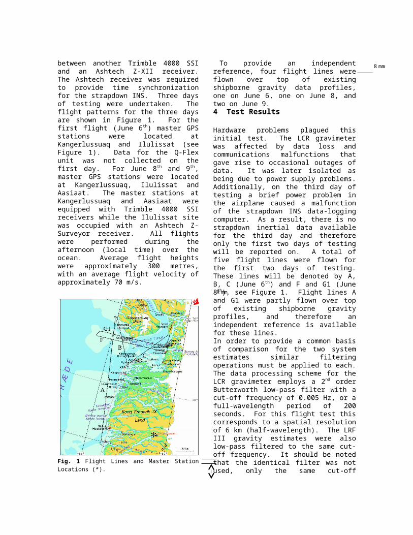
The three independent systems were mounted in a Twin Otter airplane. Two dual frequency GPS antennas were mounted on the fuselage of the aircraft. The front antenna was attached to a Trimble 4000 SSI receiver, while the rear antenna signal was split between another Trimble 4000 SSI and an Ashtech Z-XII receiver. The Ashtech receiver was required to provide time synchronization for the strapdown INS. Three days of testing were undertaken. The flight patterns for the three days are shown in Figure 1. For the first flight (June 6th) master GPS stations were located at Kangerlussuaq and Ilulissat (see Figure 1). Data for the Q-Flex unit was not collected on the first day. For June 8th and 9th, master GPS stations were located at Kangerlussuaq, Ilulissat and Aasiaat. The master stations at Kangerlussuaq and Aasiaat were equipped with Trimble 4000 SSI receivers while the Ilulissat site was occupied with an Ashtech Z-Surveyor receiver. All flights were performed during the afternoon (local time) over the ocean. Average flight heights were approximately 300 metres, with an average flight velocity of approximately 70 m/s.

Fig. 1 Flight Lines and Master Station Locations (*).

8 mm

Figures are placed

at the bottom or top of a page if

possible

2 mm

To provide an independent reference, four flight lines were flown over top of existing shipborne gravity data profiles, one on June 6, one on June 8, and two on June 9.4 Test Results

Hardware problems plagued this initial test. The LCR gravimeter was affected by data loss and communications malfunctions that gave rise to occasional outages of data. It was later isolated as being due to power supply problems. Additionally, on the third day of testing a brief power problem in the airplane caused a malfunction of the strapdown INS data-logging computer. As a result, there is no strapdown inertial data available for the third day and therefore only the first two days of testing will be reported on. A total of five flight lines were flown for the first two days of testing. These lines will be denoted by A, B, C (June 6th) and F and G1 (June 8th), see Figure 1. Flight lines A and G1 were partly flown over top of existing shipborne gravity profiles, and therefore an independent reference is available for these lines.In order to provide a common basis of comparison for the two system estimates similar filtering operations must be applied to each. The data processing scheme for the LCR gravimeter employs a 2nd order Butterworth low-pass filter with a cut-off frequency of 0.005 Hz, or a full-wavelength period of 200 seconds. For this flight test this corresponds to a spatial resolution of 6 km (half-wavelength). The LRF III gravity estimates were also low-pass filtered to the same cut-off frequency. It should be noted that the identical filter was not used, only the same cut-off frequency. Therefore, distortion due to transfer function differences between the two filters may cause discrepancies in the results. However, it is expected that this effect will be negligible compared to the overall system errors.The same DGPS position estimates were used to determine aircraft kinematic acceleration for both systems. Obviously, the position estimates must be differentiated twice to determine acceleration. KMS uses a first-order Taylor Series central difference approximation to differentiate the data. The U of C acceleration estimate is computed using a low-pass FIR differentiating filter. Bruton et al. (1999) describe and compare these two methods of differentiation. The conclusion in this reference is that the above two methods are nearly equivalent

for the frequency band of interest in airborne gravity.Therefore, differences in the estimates between the LCR and the LRF III systems should represent the combined noise levels of the two systems’ specific force estimates plus any differences due to lever arm effects (due to different measurement origins). In order to compensate for the lever-arm effect the offset between the LCR and LRF III was used along with the strapdown INS angular velocities to compute a lever arm velocity. This velocity was then differentiated to compute a relative lever-arm acceleration that was subsequently low-pass filtered to 200 seconds. The filtered lever-arm acceleration corrections were then applied to the LRF III data. The results of the comparison between the LCR and the LRF III estimates for all five flight lines are displayed in Table 1. The RMS of the differences was computed, and therefore, these values are divided by to get an idea of the standard deviation () for each measuring unit, assuming the systems have the same accuracy. It should also be noted that a linear bias has been removed between the two system estimates. The linear biases have a slope of approximately 0.01 mGal/s. This linear bias is due mostly to the behaviour of the accelerometer biases for the LRF III strapdown INS system, see Glennie (1999).

Table 1. Comparison of LCR and LRF III Gravity Estimates, in mGal (Tc = 200 sec)

Flight line RMS A 2.4 1.7B 3.0 2.1C 1.4 1.1F 7.7 4.4G1 4.0 2.9

The LCR gravimeter showed a very stable bias behaviour. Table 2 shows the RMS crossover errors for the LCR before and after applying a constant bias for each flight track for all three days of testing, based on a total of 15 crossovers. The small value of the crossover errors indicates LCR accuracies below 2 mGal, and illustrates the long-term stability of the spring gravimeter system. However, it should be noted that the low RMS after the bias adjustment is likely too optimistic due to the small number of crossovers. For all three days, a comparison of the

8 mm

Tables are also placed at the bottom or top of a page if

possible. They are in small type (8.5 pt, line spacing

3.5 mm)

8 mm

8 mm

LCR estimates to available ground truth yielded an overall RMS difference of 3.1 mGal for the unadjusted data set.

References

Bastos, L., S. Cunha, R. Forsberg, A. Olesen, A. Gidskehaug, U. Meyer, T. Boebel, L. Timmen, G. Xu, M. Nesemann, K. Hehl (1998). An Airborne Geoid Mapping System for Regional Sea-Surface Topography: Application to the Skagerrak and Azores Areas. In: Proc of International Association of Geodesy Symposia ‘Geodesy on the Move’. Forsberg R Feissel M Dietrich R (eds) Vol. 119, Springer Berlin Heidelberg NewYork, pp 30-36.

Brozena, J.M. (1992). The Greenland Aerogeophysics Project: Airborne Gravity, Topographic and Magnetic Mapping of an Entire Continent. In: Proc. Of IAG Symposium G3: Determination of the Gravity Field by Space and Airborne Methods, Springer Verlag, pp. 203-214.

Brozena, J.M., M.F. Peters and V.A. Childers (1997). The NRL Airborne Gravity Program. In: Proc. of International Symposium on Kinematic Systems in Geodesy, Geomatics and Navigation (KIS97), Banff, Canada, June 3-6, pp. 553-556.

Bruton, A.M., C. Glennie, and K.P. Schwarz (1999). Differentiation for High Precision GPS Velocity and Acceleration Determination. GPS Solutions, Vol 2, No. 4.

Foote, S.A., and D.B. Grindeland (1992). Model QA-3000 Q-Flex Accelerometer: High Performance Test Results. In: Proc. Of IEEE PLANS 92, IEEE, Piscataway, NJ, pp. 534-543.

Forsberg, R., A.V. Olesen, and K. Keller (1999). Airborne Gravity Survey of the North Greenland Shelf 1998. Kort & Matrikelstyrelsen Technical Report, in print.

Forsberg, R., and S. Kenyon (1994). Evaluation and Downward Continuation of Airborne Gravity Data – The Greenland Example. In: Proc. of International Symposium on Kinematic Systems in Geodesy, Geomatics and Navigation (KIS94), Banff, Canada, August 30- September 2, pp. 531-538.

Glennie, C., (1999). An Analysis of Airborne Gravity by Strapdown INS/DGPS. Ph.D. Thesis, UCGE Report #20???, Dept. of Geomatics Engineering, The University of Calgary.

Glennie, C., and K.P. Schwarz (1999). A Comparison and Analysis of Airborne Gravimetry Results from Two Strapdown Inertial/DGPS Systems. Accepted by: Journal of Geodesy.

Hehl, K., L. Bastos, S. Cunha, R. Forsberg, A.V. Olesen, A. Gidskehaug, U. Meyer, T. Boebel, L. Timmen, G. Xu and M. Nesemann (1997). Concepts and First Results of the AGMASCO Project. In: Proc. of International Symposium on Kinematic Systems in Geodesy, Geomatics and Navigation (KIS97), Banff, Canada, June 3-6, pp. 557-563.

LaCoste, L.J.B. (1988). The Zero-Length Spring Gravity Meter. Geophysics, 7, pp. 20-21.

Olesen, A.V., R. Forsberg and A Gidskehaug (1997). Airborne Gravimetry Using the LaCoste and Romberg Gravimeter - An Error Analysis. In: Proc. of International Symposium on Kinematic Systems in Geodesy, Geomatics

and Navigation (KIS97), Banff, Canada, June 3-6, pp. 613-618.

Schwarz, K.P., and M. Wei (1997). Inertial Surveying and INS/GPS Integration. ENGO 623 Lecture Notes, Department of Geomatics Engineering, The University of Calgary.

Schwarz, K.P., and Z. Li (1996). An Introduction to Airborne Gravimetry and its Boundary Value Problems. Lecture Notes, IAG International Summer School, Como, Italy, May 26 - June 7.

Schwarz, K.P., and M. Wei (1994). Some Unsolved Problems in Airborne Gravimetry. IAG Symposium ‘Gravity and Geoid’, Graz, Austria, September 11-17, pp. 131-150.

Valliant, H.D. (1992). The LaCoste and Romberg Air/Sea Gravity Meter: An Overview. CRC Handbook of Geophysical Exploration at Sea, 2nd Ed. Hydrocarbons, CRC Press Inc, pp. 141-176.

Wei, M., and K.P. Schwarz (1998). Flight Test Results from a Strapdown Airborne Gravity System. Journal of Geodesy, 72, pp. 323-332.

indent 4mm