3-D Seismic processing in crystalline rocks using...
122
-
Upload
truongthuan -
Category
Documents
-
view
216 -
download
0
Transcript of 3-D Seismic processing in crystalline rocks using...
3-D Seismic processing in crystalline
rocks using the
Common Re�ection Surface stack
Dissertation with the aim of achieving a doctoral degree
at the Faculty of Mathematics, Informatics and Natural Sciences
Department of Earth Sciences
University of Hamburg
submitted by
Khawar Ashfaq Ahmed
2015
Hamburg, Germany
Day of oral defense: 30.06.2015The following evaluators recommended the admission of the dissertation:Supervisor: Professor Dr. Dirk GajewskiCo-supervisor: Dr. Claudia Vanelle
ii

In the name of ALLAH, The Bene�cent, The Merciful
iii


Abstract
Seismic data from crystalline or hardrock environments usually exhibit a poorsignal-to-noise (S/N) ratio due to low impedance contrasts in the subsurface.Moreover, instead of continuous re�ections we observe a lot of steeply dippingevents resembling parts of di�ractions. The conventional seismic processing (CMPstack and DMO) is not ideally suited for imaging such type of data. Common-re�ection-surface (CRS) processing considers more traces during the stack thanCMP processing and the resulting image displays a better S/N ratio. In the lastdecade, the CRS method was established as a powerful tool to provide improvedimages, especially for low fold or noise contaminated data from sedimentary basins.The CRS stack and all attributes linked to it are obtained using a coherence-basedautomatic data-driven optimization procedure. In this research, the 3D CRSwork�ow was applying to 3D crystalline rock seismic data which were acquirednear Schneeberg, Germany, for geothermal exploration. 3D seismic imaging is thechallenge for data acquired in the hardrock environment. In 3D case, the datavolume is big and it is not easy to process. For this purpose, before processing thisbig data, the 3D CRS code has been optimized with the hybrid approach (messagepassing interface MPI with OpenMP). This makes the program run in e�cientfashion and can handle the big dataset up-to Tera-bytes with fast processing andalso the output quality of the image is same as the original 3D CRS processed image.
The CRS stack itself provided an image of good S/N ratio. However, for datafrom environments with low acoustic impedance and poor velocity information, thecoherence which is automatically obtained in the optimization procedure providesan alternative way to image the subsurface. Despite the reduced resolution, forthis data the coherence image provided the best results for an initial analysis.Utilized as a weight, the coherence attribute can be used to further improvethe quality of the stack. By combining the bene�ts of a decreased noise levelwith the high resolution and interference properties of waveforms, we argue thatthese results may provide the best images in an entirely data-driven processingwork�ow for the Schneeberg data. Because of the large number of di�ractionsin the data leading to numerous con�icting dips and crossing image patterns,stacks are di�cult to interpret. Time-migrated data helped to identify severalmajor fault structures, which coincide with geological features of the considered area.
Studies on these 3D crystalline rock data showed some interesting features whichwere not expected by the geologists. Schneeberg body was not expected before
v
survey. Conjugate faults cut through the Roter Kamm which is also a surprisingfact. The behaviour of Roter Kamm is new for geologists. This include thefaint seismic signature of the regional fault Roter Kamm. Before the 3D seismicsurvey, it was assumed to be the prominent feature. The distribution of di�ractionapexes in the time-migrated section shows a distinct high where several fracturesystems intersect. The fracture systems cross each other near the center of thisblock. If these di�ractions are the response of open fractures the area could serveas a natural heat exchanger to generate geothermal energy. This is an ongoingdiscussion whether the cracks are open or mineralized.
vi
Zusammenfassung
Seismische Daten aus dem Kristallinen oder Hardrock-Umgebungen weisenin der Regel aufgrund der niedrigen Impedanzkontraste im Untergrund einschlechtes Signal-Rausch (S/N) Verhältnis auf. Auÿerdem beobachten wir anstellevon kontinuierlichen Re�exionen viele steil abfallende Ereignisse, die sich wieDi�raktionssegmente verhalten. Die konventionelle Bearbeitung seismischer Daten(CMP-Stapelung und DMO) ist nicht idealerweise zur Abbildung dieser Art vonDaten geeignet ist. Die Bearbeitung mit dem Common-Re�ection-Surface (CRS)Verfahren betrachtet mehr Spuren als das CMP-Verfahren und das resultierendeBild zeigt ein besseres S/N-Verhältnis. In den letzten zehn Jahren wurde dieCRS-Methode als ein mächtiges Werkzeug eingeführt um verbesserte Bilder,vor allem für niedrig überdeckte oder verrauschte Daten aus Sedimentbeckenzu erzeugen. Der CRS-Stack und alle mit ihm verbundenen Attribute werdenunter Verwendung eines kohärenzbasierten, automatischen und datengesteuertenOptimierungsverfahren erhalten. In dieser Untersuchung wurde der 3D-CRS-Work�ow auf 3D seismische Daten im kristallinen Gestein angewendet, die in derNähe von Schneeberg, Deutschland für geothermische Exploration aufgezeichneterworben wurden. Seismische 3D-Bildgebung ist eine Herausforderung für die ineiner Hardrock-Umgebung erfassten Daten. Im 3D-Fall ist die Datenmenge groÿund nicht einfach zu bearbeiten. Zu diesem Zweck wird vor der Bearbeitungdieser groÿen Daten der 3D-CRS-Code mit dem Hybrid-Ansatz (Message PassingInterface (MPI) mit OpenMP) optimiert. Das erlaubt, das Programm in e�zienterArt und Weise auszuführen und die groÿe Datenmenge, die Tera-Bytes betragenkann, schnell zu bearbeiten und auch die Qualität des Outputs ist die gleiche wiedie des mit dem Original-3D-CRS bearbeiteten Bildes.
Der CRS-Stack selbst hat ein Bild mit gutem S/N-Verhältnis geliefert. Dochfür Daten von Umgebungen mit niedriger akustischer Impedanz und schlechtenGeschwindigkeitsinformationen, bietet die Kohärenz, die automatisch in derOptimierungsprozedur bestimmt wird, eine alternative Möglichkeit, den Untergrundabzubilden. Trotz der reduzierten Au�ösung für diese Daten war das Kohärenzbilddas beste Ergebnis für eine erste Analyse. Als Gewicht eingesetzt, kann dasKohärenzattribut verwendet werden, um die Qualität der Stapelung weiter zuverbessern. Durch die Kombination der Vorteile des verringerten Geräuschpegelsmit der hohen Au�ösung und den Interferenzeigenschaften von Wellenformen,argumentieren wir, dass diese Ergebnisse die besten Bilder in einem reindatengesteuerten Bearbeitungswork�ow für die Schneeberg-Daten liefert. Wegen
vii
der groÿen Anzahl der Di�raktionen in den Daten, die zu zahlreichen 'con�ictingdip' Situationen führen, sind die Stapelsektionen schwierig zu interpretieren.Zeitmigrierte Daten haben dazu beigetragen, mehrere groÿe Verwerfungsstrukturenzu identi�zieren, die mit geologischen Besonderheiten des betrachteten Bereichübereinstimmen.
Studien an diesen 3D Gesteinsdaten aus dem Kristallin zeigten einige interessanteFeatures, die von den Geologen nicht erwartet wurden. Der Schneeberg-Körperwurde vor der Erhebung der Daten nicht erwartet. Konjugierte Störungen schneidenden Roten Kamm, was auch eine überraschende Tatsache ist. Das Verhalten desRoten Kamm ist neu für die Geologen. Dies beinhaltet die schwache seismischeSignatur der regionalen Verwerfung Roter Kamm. Vor der Messung mit 3D-Seismikwurde davon ausgegangen, dass diese das hervorstechende Merkmal ist. DieVerteilung der Di�raktions-Apices in der zeitmigrierten Sektion zeigt ein deutlichesMaximum dort wo sich mehrere Bruchsysteme schneiden. Die Bruchsystemekreuzen einander nahe dem Zentrum dieses Blocks. Wenn diese Di�raktionen dieAuswirkungen o�ener Risse sind, könnte der Bereich als natürlicher Wärmetauscherdienen, um geothermische Energie zu erzeugen. Es ist gegenstand anhaltenderDiskussion ob die Risse o�en oder mineralisiert sind.
viii
Contents
1. Introduction 1
2. Theoretical background 5
2.1. 3D Seismics . . . . . . . . . . . . . . . . . . . . . . . . . . . . . . . . 52.2. Seismic data processing . . . . . . . . . . . . . . . . . . . . . . . . . . 6
2.2.1. Pre-processing . . . . . . . . . . . . . . . . . . . . . . . . . . . 82.3. Conventional processing . . . . . . . . . . . . . . . . . . . . . . . . . 112.4. Basics of the 3D-CRS Work�ow . . . . . . . . . . . . . . . . . . . . . 152.5. Seismic Migration . . . . . . . . . . . . . . . . . . . . . . . . . . . . . 19
3. Optimizing by hybrid MPI and OpenMP 27
3.1. Why Optimization? . . . . . . . . . . . . . . . . . . . . . . . . . . . . 273.2. Concurrent programming . . . . . . . . . . . . . . . . . . . . . . . . . 273.3. Concurrency and threading in C++ . . . . . . . . . . . . . . . . . . . 303.4. Thread Management . . . . . . . . . . . . . . . . . . . . . . . . . . . 313.5. Message Passing Interface (MPI) . . . . . . . . . . . . . . . . . . . . 333.6. Open Multi-Processing (OpenMP) . . . . . . . . . . . . . . . . . . . . 343.7. Hybrid approach for optimizing common-re�ection-surface-stack (3D
CRS) . . . . . . . . . . . . . . . . . . . . . . . . . . . . . . . . . . . . 373.8. Practical application (Synthetic data example) . . . . . . . . . . . . . 383.9. Discussion and conclusion . . . . . . . . . . . . . . . . . . . . . . . . 40
4. 3D Seismic imaging in crystalline rock 47
4.1. Study area (Schneeberg, Germany) . . . . . . . . . . . . . . . . . . . 474.2. Geology and tectonics of area . . . . . . . . . . . . . . . . . . . . . . 494.3. Seismic acquisition (Survey design) . . . . . . . . . . . . . . . . . . . 504.4. Acquisition parameters . . . . . . . . . . . . . . . . . . . . . . . . . . 534.5. 3D CRS processing . . . . . . . . . . . . . . . . . . . . . . . . . . . . 574.6. 3D poststack Kircho� time migration . . . . . . . . . . . . . . . . . . 604.7. Conclusions . . . . . . . . . . . . . . . . . . . . . . . . . . . . . . . . 71
5. Summary 91
6. Outlook 95
A. Electronic Supplements in DVD 97
ix

List of Figures
2.1. 3D Seismic acquisition. . . . . . . . . . . . . . . . . . . . . . . . . . . 72.2. 3D Seismic geometry. . . . . . . . . . . . . . . . . . . . . . . . . . . . 82.3. Horizontal re�ector in subsurface. . . . . . . . . . . . . . . . . . . . . 122.4. (a) NIP wave and (b) N wave. The quantities MNIP and MN
are related to wavefront curvatures associated with the hypotheticalemerging NIP and normal waves at Xo on the measurement surface. . 17
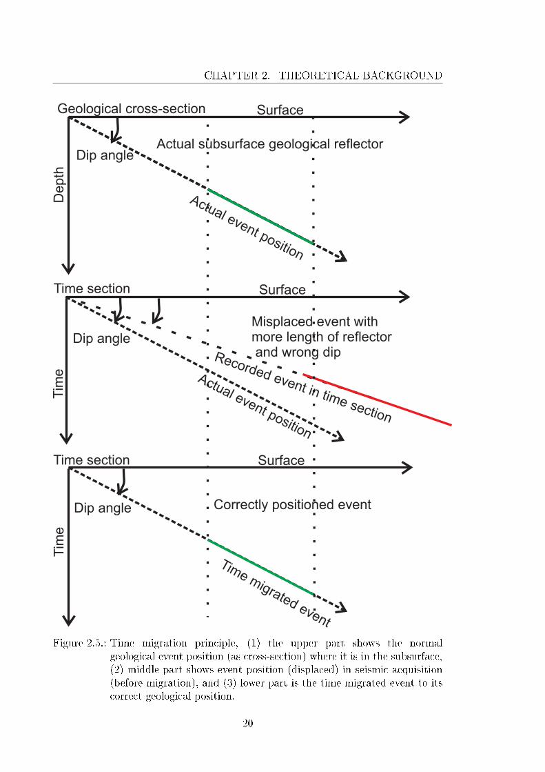
2.5. Time migration principle, (1) the upper part shows the normalgeological event position (as cross-section) where it is in thesubsurface, (2) middle part shows event position (displaced) in seismicacquisition (before migration), and (3) lower part is the time migratedevent to its correct geological position. . . . . . . . . . . . . . . . . . 20
3.1. Multi-tasking on single core and dual core machine. . . . . . . . . . . 283.2. Distributed memory architecture of machine. . . . . . . . . . . . . . . 343.3. Shared memory architecture of machine. . . . . . . . . . . . . . . . . 353.4. Generation of threads with OpenMP. . . . . . . . . . . . . . . . . . . 363.5. Graph showing the 3D CRS (express) processing with time.
(relative acceleration of the hybridized MPI+OpenMP 3D CRSimplementation as a function of number of cores) . . . . . . . . . . . 39
3.6. CMP stack section of original CRS code. . . . . . . . . . . . . . . . . 413.7. CMP stack section of hybrid CRS code. . . . . . . . . . . . . . . . . . 413.8. NIP wave radius determined by the original CRS code. . . . . . . . . 423.9. NIP wave radius determined by the hybrid CRS code. . . . . . . . . . 423.10. Angle α determined by the original CRS code. . . . . . . . . . . . . . 433.11. Angle α determined by the hybrid CRS code. . . . . . . . . . . . . . 433.12. N wave curvature determined by the original CRS code. . . . . . . . . 443.13. N wave curvature determined by the hybrid CRS code. . . . . . . . . 443.14. Coherence determined by the original CRS code. . . . . . . . . . . . . 453.15. Coherence determined by the hybrid CRS code. . . . . . . . . . . . . 453.16. CRS stack section obtained by the original CRS code. . . . . . . . . . 463.17. CRS stack section obtained by the hybrid CRS code. . . . . . . . . . 46
4.1. Study area located on geographic map. . . . . . . . . . . . . . . . . . 484.2. Regional tectonic map showing Schneeberg study area (Linnemann
and Romer, 2010). . . . . . . . . . . . . . . . . . . . . . . . . . . . . 50
xi
List of Figures
4.3. Geological map of Schneeberg study area. Coordinates specify in-lineand cross-line locations. (modi�ed after (Berger et al., 2011)) . . . . 51
4.4. Cross-section of Schneeberg study area passing near in-line 660.(Berger et al., 2011) . . . . . . . . . . . . . . . . . . . . . . . . . . . 52
4.5. Planing of acquisition lines (courtesy of LIAG, Hannover, Germany). 534.6. No-permit area indicted by purple colour. (courtesy of LIAG,
Hannover, Germany). . . . . . . . . . . . . . . . . . . . . . . . . . . . 554.7. Map of fold density of Schneeberg re�ection data (courtesy of LIAG,
Hannover, Germany). . . . . . . . . . . . . . . . . . . . . . . . . . . . 564.8. Shot gathers of hardrock (Schneeberg area, Germany) and
sedimentary rock (TGS Levantine basin, Mediterranean Sea). . . . . . 574.9. Comparison of (a) (brute) CMP stack, (b) CRS stack, (c) coherence,
and (d) coherence weighted stack (CWS) of in-line 390. . . . . . . . . 614.10. Coherence section of in-line 369. Di�erent features are pointed out
with arrow which are observed in the subsurface. . . . . . . . . . . . 624.11. Migrated 3D coherence in-line 290. . . . . . . . . . . . . . . . . . . . 644.12. Migrated coherence weighted CRS stack in-line 290. The features are
better visible than in coherence. . . . . . . . . . . . . . . . . . . . . . 654.13. Migrated 3D coherence weighted CRS stacked in-line 148. Starting
from below x-line 200, slight hint of Roter Kamm with polarityreversal. . . . . . . . . . . . . . . . . . . . . . . . . . . . . . . . . . . 66
4.14. Migrated 3D CRS stack in-line 350. In higher time 1600 - 2000 ms, thepolarity reversal is strong. The legend shows the maximum coherenceof 0.02. . . . . . . . . . . . . . . . . . . . . . . . . . . . . . . . . . . . 67
4.15. Migrated 3D stack weighted CRS stack cross-line 580. Steep dippingNE clayey schist is strong event in this section. Event nearly belowin-line 350 at time 2800 ms is also noticed which is small and dippingin north. Strong re�ection from higher time near 3200 ms is alsoobserved. . . . . . . . . . . . . . . . . . . . . . . . . . . . . . . . . . . 72
4.16. Migrated coherence time slice 1330 ms. . . . . . . . . . . . . . . . . . 734.17. Migrated coherence time slice 2010 ms. . . . . . . . . . . . . . . . . . 744.18. Migrated coherence time slice 2250 ms. . . . . . . . . . . . . . . . . . 754.19. Migrated coherence time slice 2340 ms. . . . . . . . . . . . . . . . . . 764.20. Migrated coherence time slice 2470 ms. . . . . . . . . . . . . . . . . . 774.21. Migrated coherence weighted stack time slice 1400 ms. . . . . . . . . 784.22. Migrated coherence weighted stack time slice 1120 ms. . . . . . . . . 794.23. Migrated coherence weighted stack time slice 1200 ms. . . . . . . . . 804.24. Migrated coherence weighted stack time slice 1600 ms. . . . . . . . . 814.25. Migrated coherence weighted stack time slice 1800 ms. . . . . . . . . 824.26. Migrated coherence weighted stack time slice 2020 ms. . . . . . . . . 834.27. Migrated coherence weighted stack time slice 2100 ms. . . . . . . . . 844.28. Migrated coherence weighted stack time slice 2150 ms. . . . . . . . . 854.29. Migrated coherence weighted stack time slice 2700 ms. . . . . . . . . 86
xii

4.30. Migrated coherence volume (inside structure). . . . . . . . . . . . . . 874.31. Migrated coherence weighted stack view1. . . . . . . . . . . . . . . . 884.32. Migrated coherence weighted stack view2. . . . . . . . . . . . . . . . 894.33. Migrated coherence transparency. . . . . . . . . . . . . . . . . . . . . 90
xiii

List of Tables
4.1. 3D seismic data acquisition parameters. . . . . . . . . . . . . . . . . . 544.2. Parameters used for 3D CRS stack. . . . . . . . . . . . . . . . . . . . 584.3. Parameters used for 3D Kircho� poststack time migration. . . . . . . 63
xv

1. Introduction
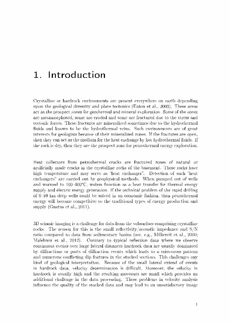
Crystalline or hardrock environments are present everywhere on earth dependingupon the geological diversity and plate tectonics (Eaton et al., 2003). These areasact as the prospect zones for geothermal and mineral exploration. Some of the zonesare metamorphosed, some are eroded and some are fractured due to the stress andtectonic forces. These fractures are mineralized sometimes due to the hydrothermal�uids and known to be the hydrothermal veins. Such environments are of greatinterests for geologists because of their mineralized zones. If the fractures are open,then they can act as the medium for the heat exchange by hot hydrothermal �uids. Ifthe rock is dry, then they are the prospect zone for petrothermal energy exploration.
Heat collectors from petrothermal cracks are fractured zones of natural orarti�cially made cracks in the crystalline rocks of the basement. These rocks havehigh temperature and may serve as �heat exchanger�. Detection of such �heatexchangers� are carried out by geophysical methods. When pumped out of wellsand warmed to 100�300°C, waters function as a heat transfer for thermal energysupply and electric energy generation. If the technical problem of the rapid drillingof 6�10 km deep wells could be solved in an economic fashion, then petrothermalenergy will become competitive to the traditional types of energy production andsupply (Gnatus et al., 2011).
3D seismic imaging is a challenge for data from the subsurface comprising crystallinerocks. The reason for this is the small re�ectivity/acoustic impedance and S/Nratio compared to data from sedimentary basins (see, e.g., Milkereit et al., 2000;Malehmir et al., 2012). Contrary to typical re�ection data where we observecontinuous events over large lateral distances hardrock data are usually dominatedby di�ractions or parts of di�raction events which leads to a criss-cross patternand numerous con�icting dip features in the stacked sections. This challenges anykind of geological interpretation. Because of the small lateral extend of eventsin hardrock data, velocity determination is di�cult, Moreover, the velocity inhardrock is usually high and the resulting moveouts are small which provides anadditional challenge in the data processing. These problems in velocity analysisin�uence the quality of the stacked data and may lead to an unsatisfactory image
1
CHAPTER 1. INTRODUCTION
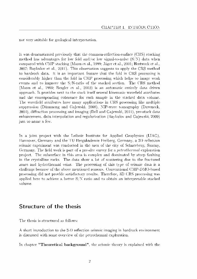
not very suitable for geological interpretation.
It was demonstrated previously that the common-re�ection-surface (CRS) stackingmethod has advantages for low fold and/or low signal-to-noise (S/N) data whencompared with CMP stacking (Mann et al., 1999; Jäger et al., 2001; Hertweck et al.,2007; Baykulov et al., 2011). This observation suggests to apply the CRS methodto hardrock data. It is an important feature that the fold in CRS processing isconsiderably higher than the fold in CMP processing which helps to image weakevents and to improve the S/N-ratio of the stacked section. The CRS method(Mann et al., 1999; Bergler et al., 2002) is an automatic entirely data drivenapproach. It provides next to the stack itself several kinematic wave�eld attributesand the corresponding coherence for each sample in the stacked data volume.The wave�eld attributes have many applications in CRS processing like multiplesuppression (Dümmong and Gajewski, 2008), NIP-wave tomography (Duveneck,2004), di�raction processing and imaging (Dell and Gajewski, 2011), pre-stack dataenhancement, data interpolation and regularization (Baykulov and Gajewski, 2009)just to name a few.
In a joint project with the Leibniz Institute for Applied Geophysics (LIAG),Hannover, Germany and the TU Bergakademie Freiberg, Germany, a 3D re�ectionseismic experiment was conducted in the area of the city of Schneeberg, Saxony,Germany. The �eld work is part of a pre-site survey for a petrothermal explorationproject. The subsurface in this area is complex and dominated by steep faultingin the crystalline rocks. The data show a lot of scattering due to the fracturedzones and hydrothermal veins. The processing of this type of seismic data is achallenge because of the above mentioned reasons. Conventional CMP-DMO-basedprocessing did not provide satisfactory results. Therefore, 3D CRS processing wasapplied here to achieve a better S/N ratio and to obtain an interpretable stackedvolume.
Structure of the thesis
The thesis is structured as follows:
A short introduction to the 3-D re�ection seismic imaging in hardrock environmentis discussed with some overview of the petrothermal exploration.
In chapter "Theoretical background", the seismic theory is explained with the
2

introduction of 3D seismic including the acquisition, preprocessing and 3D CRSprocessing. After processing, the stacked volume is also migrated.
New implementation for e�cient performance of 3D CRSprocessing
In chapter "Optimizing by Hybrid MPI and OpenMP" optimization relatedwork is discussed, as 3D CRS is costly because full attributes searches consumea lot of time compared to other processes. A hybrid parallelization approach hasbeen implemented. As the code was already MPI based, OpenMP and concurrentprogramming is introduced at some tasks without changing the major routines ofscienti�c calculation of CRS attributes. This gives a fast and robust approach toget the output of processed seismic 3D volume specially when the data is huge.
In chapter "3D Seismic imaging in crystalline rock", 3D seismic imaging ofthe Schneeberg data is presented. 3D CRS itself improved the images, but thedata volume was still not interpretable in detail. In this case, when the velocityinformation is not so good, coherence gave alternative and better interpretableimages. Because of the criss-cross pattern, the time migration is also applied inthe work �ow which helped to improve the structural interpretation. It made theinterpretation of faults and structures consistent and most features are accordingto the geological expectations.
In chapter "Summary and outlook", the results are discussed with respect tothe geophysical exploration in crystalline rock. The advantage of optimizationis discussed and the results of studies on the optimized code is elaborated. Theresultant achievement from this 3D hard rock seismic imaging via 3D CRS work�owis explained. This study show that the 3D CRS work�ow can handle such type ofdata (low coherence and S/N ratio) better than the conventional CMP processing.Also, the coherence based seismic imaging gives more information about thesub-surface structure and tectonics.
Electronic material related to this application of 3D seismic study are given inappendix.
3

2. Theoretical background
2.1. 3D Seismics
Earth itself is a 3D structure and all geological features inside the earth are threedimensional (3D) which are of great interest for the exploration. The examplesinclude duplex structures, hydrothermal veins, salt diapirs, faults and folds etc.A 2D seismic section is the response of the 3D re�ection seismic along a pro�le.Although 2D sections contain the signal from all directions, including out of planeenergy, 2D migration normally assumes that all signal originate from the plane in thepro�le. Only expert interpreter may recognize the response of signal which comesfrom out of the plane.
3D seismic surveys (data acquisition)
A typical 3D marine survey is carried out by shooting closely spaced parallel lineswhich are called shooting lines. The typical land seismic survey is carried outwith the number of parallel receiver lines which are perpendicular to the directionof shooting lines. For land 3D seismic acquisition, the source and receiver linesmay or may not be straight, depending upon the access and availability of thelocation. It also depends on the topography of the area. Also in 3D seismicacquisition, the receivers and sources can be in the form of groups designed indi�erent con�gurations and shapes according to the demand and need of thatacquisition. Di�erent types of sources can be used in data acquisition such asvibroseis, dynamite, air gun, etc.
In seismic data acquisition, a typical 3D seismic data is a group of closelyspaced seismic lines which are crossing each other and provide densely sampledmeasurements of the subsurface re�ectivity. Typical receiver line spacing can rangefrom 300 m to over 600 m, and typical distance between shot points and receivergroups is 25 m. It depends on the subsurface structure as well. If it is complex, line
5
CHAPTER 2. THEORETICAL BACKGROUND
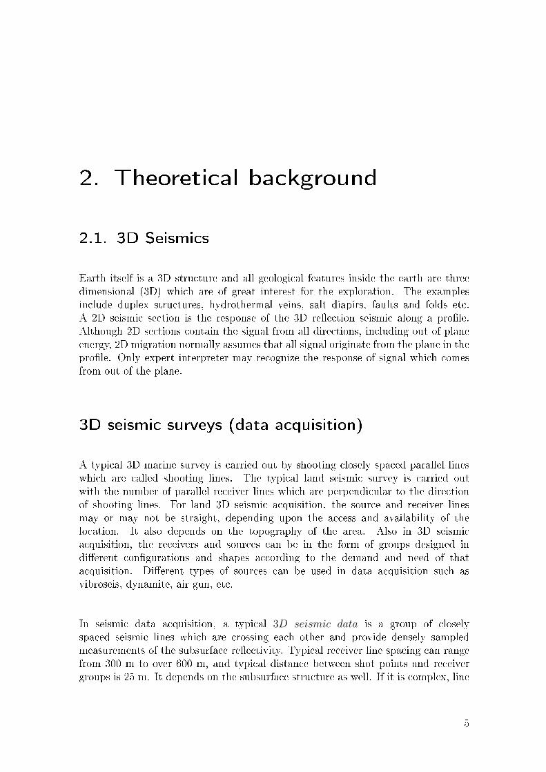
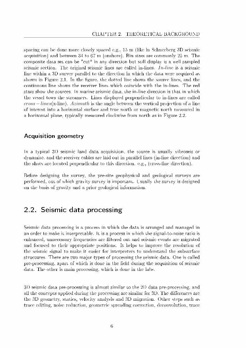
spacing can be done more closely spaced e.g., 15 m (like in Schneeberg 3D seismicacquisition) and between 34 to 67 m (onshore). Bin sizes are commonly 25 m. Thecomposite data set can be "cut" in any direction but still display is a well sampledseismic section. The original seismic lines are called in-lines. In-line is a seismicline within a 3D survey parallel to the direction in which the data were acquired asshown in Figure 2.1. In the �gure, the dotted line shows the source lines, and thecontinuous line shows the receiver lines which coincide with the in-lines. The redstars show the sources. In marine seismic data, the in-line direction is that in whichthe vessel tows the streamers. Lines displayed perpendicular to in-lines are calledcross− lines(x-line). Azimuth is the angle between the vertical projection of a lineof interest into a horizontal surface and true north or magnetic north measured ina horizontal plane, typically measured clockwise from north as in Figure 2.2.
Acquisition geometry
In a typical 3D seismic land data acquisition, the source is usually vibroseis ordynamite, and the receiver cables are laid out in parallel lines (in-line direction) andthe shots are located perpendicular to this direction. e.g., (cross-line direction).
Before designing the survey, the pre-site geophysical and geological surveys areperformed, out of which gravity survey is important. Usually the survey is designedon the basis of gravity and a prior geological information.
2.2. Seismic data processing
Seismic data processing is a process in which the data is arranged and managed inan order to make it interpretable. It is a process in which the signal-to-noise ratio isenhanced, unnecessary frequencies are �ltered out and seismic events are migratedand focused to their appropriate positions. It helps to improve the resolution ofthe seismic signal to make it easier for interpreters to understand the subsurfacestructures. There are two major types of processing the seismic data. One is calledpre-processing, apart of which is done in the �eld during the acquisition of seismicdata. The other is main processing, which is done in the labs.
3D seismic data pre-processing is almost similar to the 2D data pre-processing, andall the concepts applied during the processing are similar for 3D. The di�erences arethe 3D geometry, statics, velocity analysis and 3D migration. Other steps such astrace editing, noise reduction, geometric spreading correction, deconvolution, trace
6
So
urc
e L
ine
C
So
urc
e L
ine
A
So
urc
e L
ine
B
So
urc
e L
ine
E
So
urc
e L
ine
F
So
urc
e L
ine
G
So
urc
e L
ine
D
Receiver Line 6
Receiver Line 5
Receiver Line 4
Receiver Line 3
Receiver Line 2
Receiver Line 1
Source line
Receiver line
Source point
{
Gro
up o
f re
ceiv
er
lines
Figure 2.1.: 3D Seismic acquisition.
balancing, and statics are applied similar to the 2D surveys. One other di�erenceis the binning. In 2D the traces are collected in common-midpoint (CMP) gathers,while in 3D, it is done in terms of cells known as CMP cell or bin.
7
CHAPTER 2. THEORETICAL BACKGROUND
N
Azimuth angle
{Group of receiver lines
In-line
X-line
Source point
Source line
Receiver line
1
2
3
4
AB
C
Figure 2.2.: 3D Seismic geometry.
3D data is often visualized in so called time slices. A time slice is a horizontaldisplay or map view of 3D seismic data having a certain arrival time value, asopposed to a horizon slice that shows a particular re�ection. A time slice is a quick,convenient way to evaluate changes in amplitude of seismic data (Schlumberger,2015).
2.2.1. Pre-processing
Seismic pre-processing is a part of seismic data processing during which some stepsare usually done immediately in the �eld during the seismic data acquisition. Thisis mandatory to assure the quality control of the seismic data acquisition and toevaluate the signal quality as well. Some pre-processing steps are listed here:
� De-multiplex : this is �rst step in which the traces of seismic data is converted
8
to (SEG-Y,D) from multiplexed format (SEG-A,B).
� Re-sampling : this is done in the �eld depending upon the signal quality.Normally the standard sampling interval is 2 ms.
� Editing : trace editing is done in-order to remove dead or bad traces.
� Deconvolution : it is inverse �ltering in which the frequencies of a seismicsignal is enhanced. It improves the resolution of seismic data which is badlya�ected by the convolution process when seismic energy is �ltered by earth.
� Noise attenuation : di�erent types of noise are present in the data when it iscollected in the �eld during acquisition. This includes the ground rolls, noiseproduced by living beings, wind, electric poles etc. It is attenuated in the �eldby applying certain di�erent types of �lters.
� Multiple attenuation : Multiple is the multiply re�ected seismic energy, orany event in seismic data that has incurred more than one re�ection in itstravel path. Multiples are the part of seismic data which are observed duringseismic data acquisition. They have to be removed from the data to get agood approximation of the subsurface because most imaging methods assumeprimary only re�ection data. Usually predictive deconvolution is used toremove the multiples. Water bottom multiples and sea surface interface areobserved in common practice in marine seismic data which are suppressed byspecial seismic processing like, e.g., surface related multiples, removal (SRME),(see., Bruce et al. (2009)).
� Static correction : static corrections depend on the topography. If the areais �at, then static correction are not required. Also in marine acquisition,the static correction is not required if the tide are usually less then 6 m. Ifthe topography is rough with landscapes, then it is crucial to apply it tobring the acquisition horizons to the datum. Static corrections compensatefor di�erences in topography and di�erences in the elevations of sources andreceivers. In land seismic, it is usually common practice to remove the e�ectof weathering layer near the surface where the velocity is very low. It is alsoknown as weathering correction.
� Quality Control (QC) of data : it is done in the �eld to check the quality ofthe signal and to correct the geometry.
� 3D binning : this is a process in which seismic data is divided into small partsaccording to the mid points between the sources and receivers. This is donebefore stacking data. In standard procedures, the binning space is 25 m by 25
9
CHAPTER 2. THEORETICAL BACKGROUND
m. But if its required, the binning can be done more closely spaced accordingto the demands.
Muting is a process, to remove the contribution of selected seismic events in astack to minimize certain e�ects such as air waves, ground roll, near surface lowfrequency content or noise from �rst arrivals. The main targets of this process isthe low frequency content specially present in the early parts of the dataset.
The change of amplitudes of oscillatory signal from original available input to theampli�ed output is known as gain. It is the time variant scaling function based onthe desired criterion. For-example : geometric spreading correction is applied for thecompensation of wavefront divergence. It should be applied with great care as itsside e�ect can ruin the seismic signal. There are di�erent types of gain. The mostcommon practice used in seismic processing is automatic gain control (AGC). Thisis applied to improve the signal of the late arriving events in which the attenuationand wavefront divergence has caused the decay of the amplitude of the signal. AGCis a kind of trace equalizer as well. It balances out the amplitudes across the wholetrace. Although the AGC is fast to apply, it has downsides as well. It uses themean value on the basis of the average amplitude and no �true amplitudes� anymore.
Filtering is a procedure in which the undesired portion of the dataset is removed.This removal can be done in terms of frequency or amplitude or some otherinformation from seismic dataset. This is done for increasing the signal-to-noise(S/N) ratio. Usually �rst of all, it is used to remove the coherent noise contentfrom the data and to apply deconvolution. Sometimes, the unwanted frequencyband is removed by band pass �ltering. After pre-processing, certain �lters such aslow pass (high cut) or high pass (low cut) or band pass frequency �lter is appliedfor certain band of frequencies which are unwanted in the signal processing. Allof these �ltering (other than deconvolution) almost follow the same principle toconstruct the zero phase wavelet with �at amplitude spectrum.
The mostly applied �lter is known as a band pass �lter because seismic datamostly contains low frequency content which acts as noise, such as ground roll,and some high frequency ambient noise. Band-pass �lter is performed at variousstages in seismic data processing. If necessary, it can also be applied before thedeconvolution to suppress ground roll. Narrow band-pass �ltering is applied beforecross-correlation of traces in a CMP gather to estimate residual static shifts.
10

2.3. Conventional processing
After pre-processing of the seismic data, di�erent steps are taken into account duringthe conventional seismic processing. These include velocity analysis, gain whichcould be AGC or clipping, �ltering di�erent undesired frequencies, and then stacking.The stacking may be of di�erent kinds, like brute stack, common midpoint (CMP)stack, common re�ection surface (CRS) stack, etc. After stacking, migration ofthe stacked data is performed to bring the re�ection seismic events to their correctposition. Two major types of migration are prestack and poststack migration. Thesub-types include the time migration and depth migration.
The common-midpoint (CMP) stack
The common-midpoint (CMP) stacking was �rst time presented by (Mayne, 1962)under the assumption of a horizontally layered medium, in which the re�ection eventsmeasured on di�erent traces in a CMP gather stem from a common re�ection pointin the subsurface located directly beneath the CMP location.
t2(h) = t02 +
4h2
ν2(2.1)
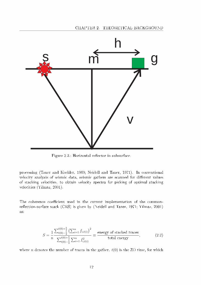
The CMP stack is a simulated zero-o�set ssection which makes use of theredundancy in multicoverage seismic data by considering traces of a commonmidpoint but with varying o�sets. Seismic signals are summed up in the form ofstack based on the coherency of traces in the o�set direction along the stackingcurves. The resultant outcome has an improved signal-to-noise (S/N) ratio whichare arranged with respect to the midpoint location. In Figure 2.3, h is the halfo�set distance. The re�ection traveltimes t(h) are measured in the CMP gatherwhich is described in the equation 2.1 . ν is the stacking velocity which describesthe least �tting moveout to the data.
Coherence is a measure of the similarity of two signals (here seismic events) ina dataset. The most commonly used coherence measure is Semblance. It is thestatistic measure between the consistency of the two seismic events. It was �rstintroduced by (Taner and Koehler, 1969). Semblance is the normalized coherencyfunction (Luo and Hale, 2012). The semblance has been an indispensable toolfor measure of velocity analysis in the seismic datasets (Fomel, 2009). Semblancebased analysis is commonly performed in velocity analysis during the seismic data
11
CHAPTER 2. THEORETICAL BACKGROUND
ms g
v
h
Figure 2.3.: Horizontal re�ector in subsurface.
processing (Taner and Koehler, 1969; Neidell and Taner, 1971). In conventionalvelocity analysis of seismic data, seismic gathers are scanned for di�erent valuesof stacking velocities, to obtain velocity spectra for picking of optimal stackingvelocities (Yilmaz, 2001).
The coherence coe�cient used in the current implementation of the common-re�ection-surface stack (CRS) is given by (Neidell and Taner, 1971; Yilmaz, 2001)as:
S =1
n
∑t(0)+ b2
t(0)− b2
(∑ni=1 fi,t(i)
)2∑t(0)+ b
2
t(0)− b2
∑ni=1 f
2i,t(i)
≡ energy of stacked traces
total energy, (2.2)
where n denotes the number of traces in the gather. t(0) is the ZO time, for which
12

Semblance S is evaluated and t(i) is the operator traveltime for (∆xm, h)i. fi,t(i)denotes the amplitude on the i-th trace for t = t(i). The stack is de�ned below:
n∑i=1
fi,t(i) (2.3)
Semblance is a normalized equality and its value ranges from 0 and 1. The drawbackof the semblance criterion is that it assumes the amplitude and phase of the waveletto be constant along the whole operator which unfortunately is not the case due toangle dependent re�ection coe�cient (Müller, 2007) and geometrical spreading. Thecoherence criteria which ful�lls the de�nition of phase and amplitude incorporationis presented by (Gelchinsky et al., 1985) which ends up with high computationaldemands for the coherence estimation.
Seismic waves travel in the earth and give the indirect measurement of thevelocity. The direct measure of velocity is only possible with the sonic logs. Theseinformation derive di�erent types of velocities e.g., interval, root mean square(RMS), normal moveout (NMO), stacking, migration and average velocities. Thestacking velocity is determined by the best �t of the operator.The 'true' medium velocity is the interval velocity. There are many factors onwhich the velocity of the medium depends. Those include the type of lithology,pore shape, pore pressure, saturation content, temperature and overburden e�ects.The stacking velocity estimation requires the data recorded at non-zero o�setsprovided by common midpoint (CMP) recording (Yilmaz, 2001).
For a single layer horizontal layer, the re�ection traveltime curve as function ofo�set is a hyperbola as given in equation above. The di�erence between the twoway travel time at the given o�set and the two way travel time at the zero o�set iscalled normal moveout (NMO). The velocity required to correct the normal moveoutis called normal moveout (NMO) velocity. In case of single horizontal re�ector, thenormal moveout velocity is the velocity above the re�ector. In case of dippingre�ector, the normal moveout velocity is velocity of medium divided by the cosineof the dip angle as given:
VNMO =ν0
cosφ(2.4)
If the re�ector is observed in three dimensions, then there is additional a factor
13
CHAPTER 2. THEORETICAL BACKGROUND
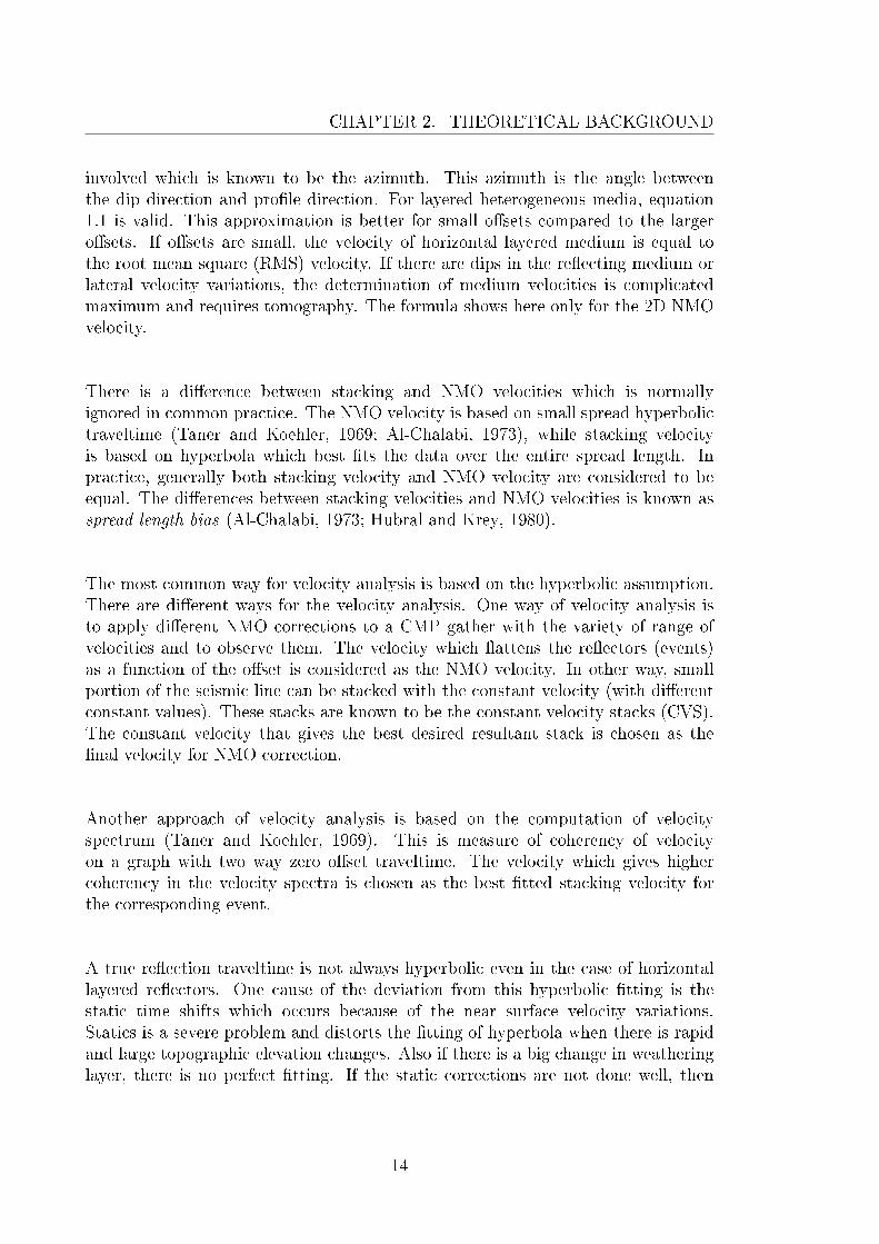
involved which is known to be the azimuth. This azimuth is the angle betweenthe dip direction and pro�le direction. For layered heterogeneous media, equation1.1 is valid. This approximation is better for small o�sets compared to the largero�sets. If o�sets are small, the velocity of horizontal layered medium is equal tothe root mean square (RMS) velocity. If there are dips in the re�ecting medium orlateral velocity variations, the determination of medium velocities is complicatedmaximum and requires tomography. The formula shows here only for the 2D NMOvelocity.
There is a di�erence between stacking and NMO velocities which is normallyignored in common practice. The NMO velocity is based on small spread hyperbolictraveltime (Taner and Koehler, 1969; Al-Chalabi, 1973), while stacking velocityis based on hyperbola which best �ts the data over the entire spread length. Inpractice, generally both stacking velocity and NMO velocity are considered to beequal. The di�erences between stacking velocities and NMO velocities is known asspread length bias (Al-Chalabi, 1973; Hubral and Krey, 1980).
The most common way for velocity analysis is based on the hyperbolic assumption.There are di�erent ways for the velocity analysis. One way of velocity analysis isto apply di�erent NMO corrections to a CMP gather with the variety of range ofvelocities and to observe them. The velocity which �attens the re�ectors (events)as a function of the o�set is considered as the NMO velocity. In other way, smallportion of the seismic line can be stacked with the constant velocity (with di�erentconstant values). These stacks are known to be the constant velocity stacks (CVS).The constant velocity that gives the best desired resultant stack is chosen as the�nal velocity for NMO correction.
Another approach of velocity analysis is based on the computation of velocityspectrum (Taner and Koehler, 1969). This is measure of coherency of velocityon a graph with two way zero o�set traveltime. The velocity which gives highercoherency in the velocity spectra is chosen as the best �tted stacking velocity forthe corresponding event.
A true re�ection traveltime is not always hyperbolic even in the case of horizontallayered re�ectors. One cause of the deviation from this hyperbolic �tting is thestatic time shifts which occurs because of the near surface velocity variations.Statics is a severe problem and distorts the �tting of hyperbola when there is rapidand large topographic elevation changes. Also if there is a big change in weatheringlayer, there is no perfect �tting. If the static corrections are not done well, then
14
the stacking velocity model for the near surface corresponding to those CMPs isunreliable.
Once the data is sorted into common cell gathers like CMPs or bins, velocityanalysis is performed. In this whole procedure, there is no di�erence between the3D velocity analysis compared to the 2D except one additional dimension for 3Dcase. The velocity analysis could be performed in certain intervals, e.g., every500 m and also for every single CMP.
Once the normal moveout (NMO) velocity is estimated, the moveout is corrected.The NMO correction needs to be done prior to the trace summation of the CMPgathers. The normal moveout depends on many factors such as velocity abovethe re�ector, o�set, zero o�set two way travel time, dip of the inclined/dippingre�ector, azimuth of the acquisition geometry (azimuth of source, and receiver)with respect to the true dip of the re�ector, and the degree of the complexity of thenear surface and medium above the re�ector.
If there is any frequency distortion in any event during NMO correction, its knownto be the NMO stretch. It occurs during the NMO correction of shallow events orthe events at large o�sets. This can severely disturb the subsurface imaging in thelarge o�sets or shallow events which are stretched. The only way to deal with itis to mute the stretched events to get rid of this problem. The threshold can bede�ned according to a certain percentage of signal stretch.
2.4. Basics of the 3D-CRS Work�ow
The CRS stack (Mann et al., 1999; Jäger et al., 2001) was originally developed toobtain simulated zero-o�set (ZO) sections or volumes from seismic multi-coveragedata. The method is based on a stacking operator that is of second order in themidpoint and half-o�set coordinates xm and h, i.e., it is of hyperbolic shape. TheCRS stacking operator at a given zero-o�set location (x0, t0) is determined by anumber of parameters related to the coe�cients of the second order traveltimeexpansion. For each zero-o�set sample to be simulated, the optimum stackingoperator is found by varying these parameter values within prede�ned boundaries.The main attributes of this work�ow are angle, normal incidence point curvatureand normal wave curvature. These parameters or attributes de�ne the shape ofthe operator. Stacking along this operator and performing a coherence analysis in
15
CHAPTER 2. THEORETICAL BACKGROUND
the pre-stack domain provides the attributes with the best �t to the data. Theparameters which yield the highest coherence value describe the optimum stackingoperator. The parameters are called kinematic wave�eld attributes (Hubral, 1983).The travel time operator for the 3D-CRS is de�ned later on.
Automatic CMP stack
The �rst step in (non-conventional stacking procedure) 3D common-re�ection-surface (CRS) stack is the generation of the automatic CMP stacked section. Theprocedure is similar to the conventional CMP stacking where the velocities aremanually picked which is based on the highest achieved coherence values betweenthe hyperbolas and recorded data. The CRS also follows the same criteria, but inautomatic way of picking of highest coherence value. Here the stacking velocitiesare de�ned in terms of ν0, α, Mnip and t0.
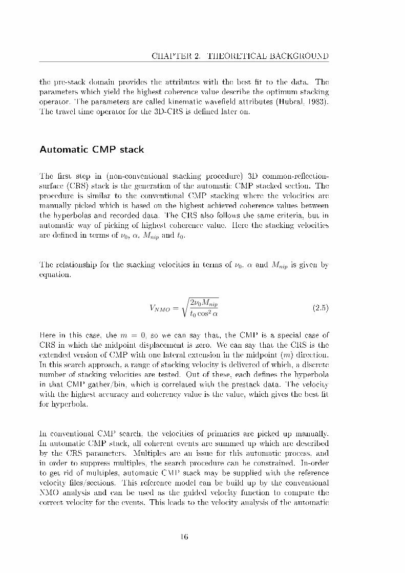
The relationship for the stacking velocities in terms of ν0, α and Mnip is given byequation.
VNMO =
√2ν0Mnip
t0 cos2 α(2.5)
Here in this case, the m = 0, so we can say that, the CMP is a special case ofCRS in which the midpoint displacement is zero. We can say that the CRS is theextended version of CMP with one lateral extension in the midpoint (m) direction.In this search approach, a range of stacking velocity is delivered of which, a discretenumber of stacking velocities are tested. Out of these, each de�nes the hyperbolain that CMP gather/bin, which is correlated with the prestack data. The velocitywith the highest accuracy and coherency value is the value, which gives the best �tfor hyperbola.
In conventional CMP search, the velocities of primaries are picked up manually.In automatic CMP stack, all coherent events are summed up which are describedby the CRS parameters. Multiples are an issue for this automatic process, andin order to suppress multiples, the search procedure can be constrained. In-orderto get rid of multiples, automatic CMP stack may be supplied with the referencevelocity �les/sections. This reference model can be build up by the conventionalNMO analysis and can be used as the guided velocity function to compute thecorrect velocity for the events. This leads to the velocity analysis of the automatic
16
CMP stack which is constrained.
3D-Common-Re�ection-Surface Stack
In the 3D case the 3D CRS operator (Bergler et al., 2002; Müller, 2003) reads:
t2(∆xm, h) = (t0 + p∆xm)2 + 2t0(∆xT
mMn∆xm + hTMniph)
(2.6)
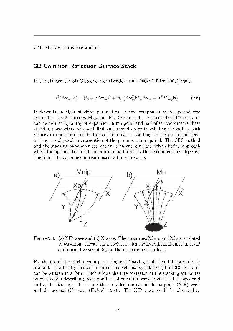
It depends on eight stacking parameters: a two component vector p and twosymmetric 2 × 2 matrices Mnip and Mn (Figure 2.4). Because the CRS operatorcan be derived by a Taylor expansion in midpoint and half-o�set coordinates thesestacking parameters represent �rst and second order travel time derivatives withrespect to mid-point and half-o�set coordinates. As long as the processing staysin time, no physical interpretation of the parameter is required. The CRS methodand the stacking parameter estimation is an entirely data driven �tting approachwhere the optimization of the operator is performed with the coherence as objectivefunction. The coherence measure used is the semblance.
Xo
Z
Y
a)
Xo
Z
Y
b)
X X
Mnip Mn
Figure 2.4.: (a) NIP wave and (b) N wave. The quantitiesMNIP andMN are relatedto wavefront curvatures associated with the hypothetical emerging NIPand normal waves at Xo on the measurement surface.
For the use of the attributes in processing and imaging a physical interpretation isavailable. If a locally constant near-surface velocity v0 is known, the CRS operatorcan be written in a form which allows the interpretation of the stacking attributesas parameters describing two hypothetical emerging wave fronts at the consideredsurface location x0. These are the so-called normal-incidence point (NIP) waveand the normal (N) wave (Hubral, 1983). The NIP wave would be observed at
17
CHAPTER 2. THEORETICAL BACKGROUND
x0 if a point-source were placed at the NIP of the zero-o�set ray on the re�ectorin the subsurface, while the N wave would be obtained if an exploding re�ectingsurface -the CRS- were placed around the NIP in the subsurface. Because of thelink to wavefront curvatures the stacking parameters are also called kinematic wave-�eld attributes. I will use both terms synonymously. The relation of the stackingparameters to the kinematic wave-�eld attributes is given by the following relations:
pm =1
v0(cosα sin β, sinα cos β)T (2.7)
Mnip =1
v0HKnipH
T (2.8)
Mn =1
v0HKnH
T (2.9)
where α is azimuth, β is dip angle andH is the 2×2 upper left sub matrix of the 3×3transformation matrix from the wavefront coordinate system into the registrationsurface. pm is the slowness vector. The 3D CRS stack is just one product of themethod next to the simulated ZO section and a number of volumes containing theoptimum kinematic wave�eld attributes and coherence for each ZO sample.
Search strategy and aperture selection during 3D CRSprocessing
During the 3D CRS processing, the aperture selection is very important, as theproper aperture setting is very crucial to get the reliable image of the subsurface.It has been observed that the validity of the determination of the proper parametersearch decreases with increasing the value of aperture distance in midpoint and o�setdirections. Appropriate choices of parameters (especially apertures) are necessary toestimate reliable attributes. If the apertures are too large the hyperbolic assumptionis no longer valid. Small apertures lead to a declined quality of the CRS attributesbecause of decreased sensitivity. The apertures for the parameter searches can bechosen separately in individual steps. Depending upon the expected subsurfacestructure, larger apertures may improve the results of the CRS attributes, whilesmaller apertures can help to avoid smearing e�ects by stacking (Baykulov, 2009).The 3D CRS attributes can be updated by an optimization. Pragmatic approachis the option for optimizing the attributes. Simulated annealing is the best suitabletechnique used for solving the optimization problems where the desired goal is hiddenamong poor, local extrema (Müller, 2003). The implementation of the simulatedannealing used in the 3D CRS optimization is the modi�cation of downhill simplex or
18
amoeba method or Nelder�Mead method or �exible polyhedron search (Nelder andMead, 1965) which is designed to �nd local minimum. The simplex is the polyhedroncomprising N+1 vertices in the N-dimensional search space. In case of 2D, it is atriangle and in 3D it is tetrahedron. The search must start from N+1 points de�ningthe simplex. At each vertex, the objective function (here coherence) is evaluatedand depending on the value of this simplex, it takes the steps for alteration of shape,size and orientation of simplex, moving towards the local minimum in N-dimensionalsearch space. The improved searched values are replaced by the old values updatingwith the highest objective function when the criteria is reached for optimal value ofcoherence. Usually this is an expensive computational process, therefore it was notused in the frame of this work. If the CRS parameters are chosen carefully and �tthe curves best, then the optimized results are similar to the non-optimized CRSparameters.Since the stack provides an image of the subsurface which does not resemble theexact geological dips and structures further processing like migration is required.
2.5. Seismic Migration
Migration is a step in seismic processing where the recorded seismic signals aremoved to their correct position in time or space. Migration moves a dippingre�ector to its true subsurface position and collapses the di�racted energy, whichresults in an increase in spatial resolution and provides a more realistic subsurfaceimage. The main purpose of the migration is to stack the data according to thesubsurface geologic cross-section either in time or in depth along the seismic traverseor volume. Mostly, the migrated seismic section is displayed in time because correctdepth requires an accurate velocity model, which is not always available. Theother reason is that it is easy to compare the stacked and time migrated sectionsbefore and after migration and it is easy for interpreters to better judge about thesubsurface structure through the seismic section. In case of poor information ofsub-surface velocities, it is preferred to keep both sections in time to get bettercomparison.
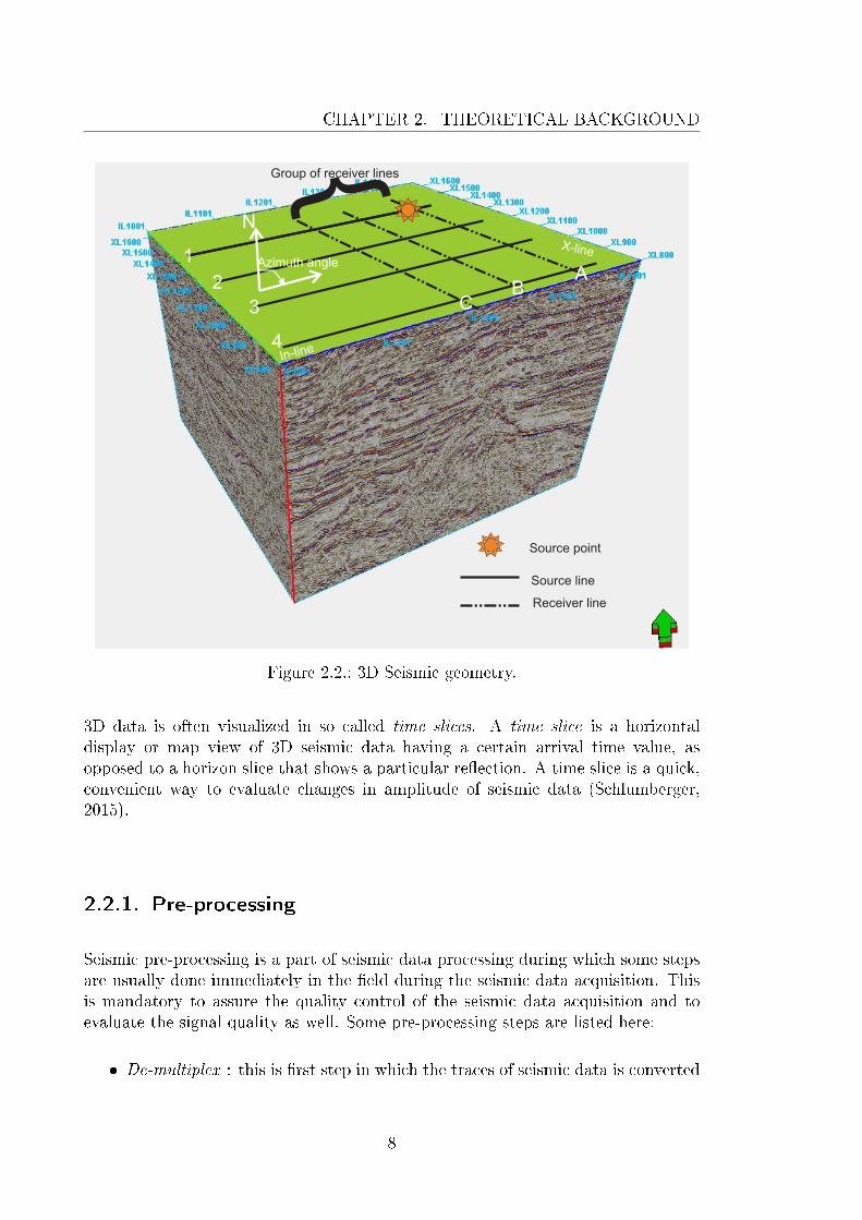
The migration which gives the output seismic section in time is known as timemigration as in Figure 2.5. This �gure gives the general conceptual idea of howmigration works, and how the events are moved during migration. It is alwaysimportant to have a clear strategy before applying migration. For every type ofdata and subsurface, there are di�erent migration tools, and di�erent migrationalgorithm works better for di�erent types of subsurface structures. A strategy formigration also includes the choice of prestack versus poststack migration or timeversus depth migration. Also, there should be appropriate parameters for migration
19
CHAPTER 2. THEORETICAL BACKGROUND
Surface
Actual subsurface geological reflector
Surface
Surface
Tim
eT
ime
Actual event position
De
pth
Actual event position
Recorded event in time section
Time migrated event
Dip angle
Dip angle
Dip angle
Misplaced event withmore length of reflectorand wrong dip
Geological cross-section
Time section
Time section
Correctly positioned event
Figure 2.5.: Time migration principle, (1) the upper part shows the normalgeological event position (as cross-section) where it is in the subsurface,(2) middle part shows event position (displaced) in seismic acquisition(before migration), and (3) lower part is the time migrated event to itscorrect geological position.
20
algorithm to work properly. Another important factor in migration is the migrationvelocity model which should be accurate. If the velocity function has errors, it couldlead to wrong placement of the events and could end up in a mis-migrated seismicsections or volumes. Suppose if there is an error of 20% in the velocities, then theevent may be misplaced by the error of 44% (Yilmaz, 2001) like shown in Figure 2.5.
Migration results in :
∗ moving the dipping events to updip,
∗ focusing di�ractions from faults, pinch-outs, edges and discontinued re�ectors,
∗ removes the e�ects of re�ector curvature such as increased anticlines, decreasedsynclines and �bow-ties� (triplication) (Stolt, 2002).
Migration Algorithms
Migration algorithms are mostly based on the scalar wave equation which arecommon in use. These algorithms handle the re�ections and multiples as seismicsignals. Any such kind of energy like noise, surface waves, and multiples areconsidered as the primary re�ections. Migration algorithms are considered intocertain categories which are based on:
∗ integral solution to scalar wave equation,
∗ frequency-wave number representation,
∗ �nite di�erence solution.
But, no matter which migration algorithm is used for data from hardrockenvironments, it should ful�ll the criteria:
∗ handle the steep dipping events accurately,
∗ be able to handle the lateral and vertical velocity variations,
∗ should be robust and e�cient,
21
CHAPTER 2. THEORETICAL BACKGROUND
∗ should be easy to implement.
There were three main era's in the history of seismic migration. First, in historicaltime before computer age, the �rst technique was developed which is known to besemicircle superposition method. Then there was a development of other techniqueknown to be the di�raction-summation technique. The migration which movesdipping events by summation of di�ractions is well known as Kirchho� Migration.Kirchho� Migration is the most �exible migration algorithm and can be easilyimplemented and used in 2D and 3D, prestack and poststack and as a time ordepth migration. Kirchho� migration can also be implemented and used to migrateshear and converted waves, apply a dip �lter, interpolate the input data andcope with spatially aliased data. Kircho� migration is commonly used. Kircho�summation was introduced by Schneider (1978), which was already in use before,during the times of di�raction summation technique with added amplitude andphase corrections applied to the data before summation (Yilmaz, 2001).
Another migration technique for zero o�set data (Claerbout and Doherty, 1972)is based on the idea that a stacked section can be modeled as an upcomingzero-o�set wave�eld which is generated by the exploding re�ector. By use ofthis model of exploding re�ector, the migration concept is considered to bethe wave�eld extrapolation in the form of downward continuation followed byimaging. Downward continuation of wave�eld can be used conveniently using the�nite di�erence solutions to the scalar wave equation. The migration which isimplemented based on such type of solutions is known to be the �nite-di�erencemigration (Claerbout, 1985).
(Stolt, 1978) introduced another method of migration which is based on the Fouriertransform. This method involves the coordinate transformation from frequency tovertical wavenumber axis while keeping the horizontal wavenumber unaltered. LaterStolt and Benson (1986) gave practical implementations together with theoreticallessons in �eld of migration with emphasis on frequency wavenumber methods.
One more way to express the frequency-wavenumber migration is the phase-shiftmethod which is purely based on downward continuation to a phase shift infrequency-wavenumber domain (Gazdag, 1978).
Out of all of the migration algorithms, none of them meets the criteria which fullycover the problems of the industry in migrating the data. So, the industry hasto depend on di�erent algorithms according to their needs and requirement in
22
handling their problems to resolve. Like one algorithm which is based on integralsolution of scalar wave equation which is known to be the Kircho� time migration.This is able to handle the steep dips up to 90◦ angle.
Other algorithm known as �nite-di�erence time migration algorithms can handleall types of the velocity variations. But they have a certain limit in handling thedegree of steepness of the dip of a seismic re�ector.
In the end, the frequency-wavenumber algorithms have limited ability in dealingwith the velocity variation especially in lateral extent. So, as a result, none of themigration algorithm in particular is able to cope with all types of problems.
Reverse time migration (RTM) (Levin, 1984) propagates the source wave�eldthrough the model and back-propagates the measured receiver wave�eld as a newsource wave�eld. In most of the cases, the ability to make use of these complexwave �eld models allow imaging of events of the subsurface that otherwise havepoor direct illumination. This migration is the most expensive method of all othermigration algorithms but provides superior images.
Migration parameters
After the decision of migration algorithm to be used, the geophysicist need to setthe appropriate parameters for the correct migration, like the Kircho� migration. Aproper aperture size matters a lot. If the aperture is smaller, then it can result inthe removal of steep dips in output migrated seismic sections. Also smaller aperturecreate the undesired horizontal events with the random noise in migrated seismicsection.
In downward continuation migration algorithm, the depth step size is an importantparameter in �nite di�erence methods. Its setting is dependent on the dip, velocity,spatial and temporal sampling and frequency in the wave �eld.
In Stolt or phase shift migration, the stretch factor is important. If the velocity isconstant, then the stretch factor is considered to be 1. In general, the larger thevertical velocity gradient, the smaller the stretch factor is needed.
23

CHAPTER 2. THEORETICAL BACKGROUND
Requirement for the data
For migration input section, there are requirements depending upon the desires bythe interpreters. Various aspects include :
∗ length of seismic line or volume of seismic line,
∗ signal-to-noise ratio (S/N) of input,
∗ spatial aliasing,
If the subsurface contains steep dipping re�ectors, then the line length must belong enough to let the steep dipping event to migrate to its actual true subsurfaceposition. If the recording length is short, then it will lead to erroneous migratedresults. In case of 3D, the surface area in x,y direction should be larger then thetarget depth of the subsurface structure (Yilmaz, 2001).
Migration velocities are very important as well as the aperture size. As the velocityincreases with increasing depth, the deeper parts are more likely to be error pronethen shallow parts. Another important point is that, the steeper the event, moreappropriate migration velocities are needed to migrate that event, as the migrationdisplacement is proportional to the dip of the event.
Theoretically the di�ractions extend to in�nite time and space. In practice, it isdi�erent and the amplitude is �nite and the aperture is chosen over which thesummation is done. The aperture may be measured in distance or traces and shouldbe large enough to include the largest lateral movement from the highest velocityand steepest dip in the section. Insu�cient aperture will cause dip limitation.Too wide aperture may slightly increase run time and may introduce noise. Ifthe stationary point is known the optimal aperture is the size of the �rst Fresnel zone.
Kircho� time migration can handle steep dipping events. The events with dip up-to90◦ is also possible to migrate. In special cases, in Kircho� depth migration, eventhe option of turning rays is possible to incorporate for migration.
The 3D Kircho� time migration is used to migrate the 3D seismic data fromSchneeberg crystalline rock environment. The main reason of choosing thismigration is that, this can handle most of the problems in migrating such dataset.However, there was no proper migration velocity model available for migrating this
24

dataset and this algorithm can handle the migration with constant velocity whenthere is are lateral velocity variations. This tool is not as expansive as RTM andgives the reasonable migrated output.
Since CRS processing is heavy in computing times some optimizations wereintroduced into the computer code. This is discussed in the next section.
25

3. Optimizing by hybrid MPI and
OpenMP
3.1. Why Optimization?
3D CRS processing has many problems in terms of e�ciency. It is expansive when8-parameters search is performed. The code used in this work was initially writtenby (Müller, 2003). This code, however, was not suited to handle the big datavolume. This is because of the reason that it is not well written for e�cientperformance and better memory usage. These all together make the data handlingand processing di�cult for seismic data processor. To resolve this issue, it wasan experimental trial to optimize the code to make it run faster for processingbig dataset. To implement this optimization, concurrent programming and hybrid(MPI + OpenMP) was introduced in the code where it is necessary. The most coste�ective routine in the code is semblance search routine, which is utilizing more then90% of the CPU time. The concurrent programming routines were applied at someroutines to the data input and output and the hybrid optimization approach to thesemblance search.
3.2. Concurrent programming
Concurrency is the property of the system in which two or more processes areoccurring simultaneously, interacting with each other. In terms of computers,it means di�erent independent activities are performing on a single systemsimultaneously instead of sequentially or one after each another. In the past, therewere computer systems which only had a single core or processor which only allowsa single task to be performed. Now-a-days, most of the systems are equipped withmulti-processors, i.e., they have more then one CPU and can perform more then onetask at the same time. Such type of machines are able to perform multiple taskssimultaneously on di�erent cores. The procedure which handles di�erent tasks isknown as task-switching. Performing more then one task on these processors is
27

CHAPTER 3. OPTIMIZING BY HYBRID MPI AND OPENMP
called multi-tasking.
Computers with multiple processors have been used as servers and clusters for highperformance computing (HPC) tasks for a number of years. These machines havemultiple cores on chips which are used in multi-tasking. Such like (multi-cores) morethen one core on the single chip is also becoming common in small machines anddesktops these days. Whether the machine has multiple processors or multiple coreson single processor (or both), such machines are capable of running multiple tasksin parallel. This type of concurrency is known to be hardware concurrency.
In computer machines, a thread is the smallest executable programmed instructionwhich can be performed independently on the operating system scheduler accordingto the programmed task. Figure 3.1 shows two types of tasks on di�erent hardwareto explain concurrency. One part (a) describes the concurrency in single core and (b)describes multiple tasks on multiple cores. On single core machine, task switchingis done and chunks from di�erent tasks are interleaved. On a dual core machine orwith more cores/CPUs, each task can be executed on its own core. Although theavailability of the concurrency in the hardware is obvious with multi-core systems,these days, some processors are available which can execute multiple threads ona single core. This is important to consider those hardware based threads whichcan measure how many tasks can be executed in parallel with the hardware. Taskswitching in this case is also easy, but parallel execution is more robust and e�cient(Williams, 2012). In workstations and desktops or laptops with single cores, thereare several tasks running even when the machine idles. This is because of the taskswitching.
Core 1
Core 2
Core2duo {
Single core
Figure 3.1.: Multi-tasking on single core and dual core machine.
28
Concurrency with multiple processes
Before going into the concurrency of programming, the most important point isto evaluate the program and try to identify which parts need the concurrency (ifthe program is already available). Then one has to analyse which parts of theprogram can be parallelized and which need task switching. This makes easier tomove towards the solution to the problem of writing a concurrent program. The�rst way to make the program concurrent is to divide it into separate multiplesingle threaded processes that are executing and running concurrently at the sametime. These threads could communicate with each other and with the main threadof the program. There is one weak point in this threading that they can executesimultaneously and interfere each other if not well programmed. This can make theprocess slow or even can halt the machine.
Concurrency for performance
Machines with multiple cores are existing for many decades, but in that time, theywere available only in supercomputers, mainframes and large server systems. Thesedays, 2, 4, 8 and 16 cores processors are easily available on a single chip andmanufacturers are improving performance daily. As a result, multi-core systems areavailable as desktops, laptops and other small machines having a single chip withmultiple processors, which are able to execute multiple tasks in parallel. If a codeneeds to take advantage of this multiple cores processors, they have to execute thetasks in parallel concurrently. There are two di�erent ways to achieve concurrency.One is to divide the task into small parts and run those in parallel. This is knownas task parallelism. It is quite complex and tricky. Di�erent factors are kept intoconsideration while dividing the tasks into parallel threads. There is another way inwhich the code performs the same work on di�erent parts of the data. This is knownas data parallelism. The codes which are able to perform such tasks of parallelismare called parallel tasks.
Concurrency in coding
In order to get the code optimized and concurrent, programmers should have thecomplete knowledge of code. Be aware of the parts of the code which have tobe parallelized and which should not. In some cases, its simple but sometimes,it is complex to dicide which parts should be parallelized. If the complexity inprogramming is high, it may end in bugs or hangups of the machines. Mostlyconcurrent code is not easy to understand and to deal with. Sometimes, its cost to
29
CHAPTER 3. OPTIMIZING BY HYBRID MPI AND OPENMP
convert from sequential to parallelized code and to run the code exceeds then theperformance increment of output. The performance may not be as e�cient accordingto expectations. One of the reason is that the task run generates too many threads,then it consumes the resources of machines and can result in making the wholesystem to process slower. This can exhaust the available memory and space for theprocess because threads require certain space for execution and communication.
The use of concurrency for performance is just like any other optimization strategy,where it has great potential to improve the performance of the code/application.On the other hand, if it is done wrong, it can lead to the complication of code whichis harder to understand and the chances of bugs increase depending upon the codecomplexity. Therefore, it is only worth-wile when applied to the critical parts of thecode for performance gains which need to be designed to optimize.
3.3. Concurrency and threading in C++
In 1998, the C++ standard does not acknowledge the thread's existence. So, it wasnot possible to make any thread execution in that compiler until 2000. Now, C++standard is fully equipped with the thread generating libraries as well as memorymodels on which the threads are dependent. Supporting concurrent programmingis one of the changes C++ compiler has in it new standards. There are di�erenttypes of compiler these days which are advanced and can deal with the paralleltasking better.
A compiler is a computer program (or set of programs) that transforms source codewritten in a programming language (either C/C++, Matlab, Java, Fortran, or anyother etc) into binary language which is machine readable to make the source codeexecutable. When running the compiler for building the executable, the compiler�rst parses (or analyzes) all of the language statements syntactically and criticallyone after the other and then, in one or more successive stages or "passes", buildsthe output code, making sure that statements that refer to other statements arereferred to correctly in the �nal code. The output code is the object code which isexecutable. The object code is machine code (binary language converted which canunderstand the code in terms of machine language) that the processor can processor "execute" one instruction of code at a time.
30
E�ciency in C++ threaded library
One of the important aspect for developers is that C++ libraries provide facilitiesof performance based e�ciency of programing routines. It gives reasonablycomprehensive facilities for concurrency and multi threading. Every given platformhas its speci�c routines to go beyond those for implementation. It is necessary tounderstand what the standard libraries provides with its facilities.
For the simple case, how to generate a simple thread with a small program example,lets have a look at the simple code written below, which shows how to incorporatethe threading in simple programs. Below is one example in which the idea is givenhow to include the thread library in a simple code. As normal routine programs, itsincluded in header. The program shows how to generate a single thread in simpleprogram. The program shows that there are thread libraries in C++ compilers whichif we include library in our program and then we can assign the task to generatethreads at certain level, and then they can perform multi-tasking.
#include <iostream>
#include <thread>
void crs()
{
std::cout<<"CRS Express\n";
}
int main()
{
std::thread t(crs);
t.join();
}
3.4. Thread Management
In concurrent programming, threads will be used to make the code working withan optimal performance. So, the �rst point is how to generate the thread. This canbe perform easily in C++ with its standard library like below given when includingin the header of a standard program:
#include <thread>
31
CHAPTER 3. OPTIMIZING BY HYBRID MPI AND OPENMP
This will make the program able to incorporate the threads if inside the threads"call" is implemented. The thread call is a trigger to generate thread by calling itwhile executing program.
Basic thread management
Generally every C++ program is running on at least a single thread which performsits task, and which is started by standard C++ run-time : main(). But the programcan generate threads in addition to this. This thread can run concurrently with themain thread. The program exits when it completes the task or the thread.
Launching thread
Threads are launched by constructing the "std::thread" object that de�nes a taskto perform by thread. If the thread is simple, then it performs tasks easily andit does not need returning. But in complex programming, it also needs someadditional routines and parameters. In the complex case, it has to perform certaindi�erent tasks independently through some communication system between thethread systems to perform a number of tasks assigned to threads. Once the threadis launched, it stops when it joins back or becomes single, or orders to stop. TheC++ thread library boils down in construction of std::thread object:
void semblence_search()
std::thread my_thread(semblence_search);
For thread, it has to be decided in the start whether to wait for it to �nish byjoining, or to leave it to run on its on by detaching it. If one does not decide beforethe thread is destroyed, then the program terminates. It is of vital importance toensure that the thread is joined or detached correctly. Another worth-wile point tonote is, if the thread is not �nished before it joins or detached, it runs for a longtime after the object of the program is destroyed. If we don't wait for the thread to�nish, then it should be ensured that the data accessed and processed by the threadis valid available unless the thread �nishes the program and tasks to complete.
32
Multithreading in C++
There are two important components in parallel programming. One is MessagePassing Interface (MPI) and other is OpenMP.
3.5. Message Passing Interface (MPI)
Message Passing Interface (MPI) is a standard portable communication systemdesigned by researchers to apply for parallel tasks on a wide variety of computers.The �rst MPI standard was presented in "Supercomputing conference 93" inNovember 1993. It is a language independent communication protocol which isused to program parallel computing systems. The goal of MPI is to provide highperformance computing (HPC) and concurrency. It is the most dominant platformused for high performance computing in super computers and clusters these days.MPI implementation comprises of di�erent set of routines which can be directlycalled from C, C++, Fortran, and Matlab and certain other languages. It has beenimplemented for di�erent memory architectures. Its implementations are optimizedroutines in di�erent sets of hardware.
Working with MPI
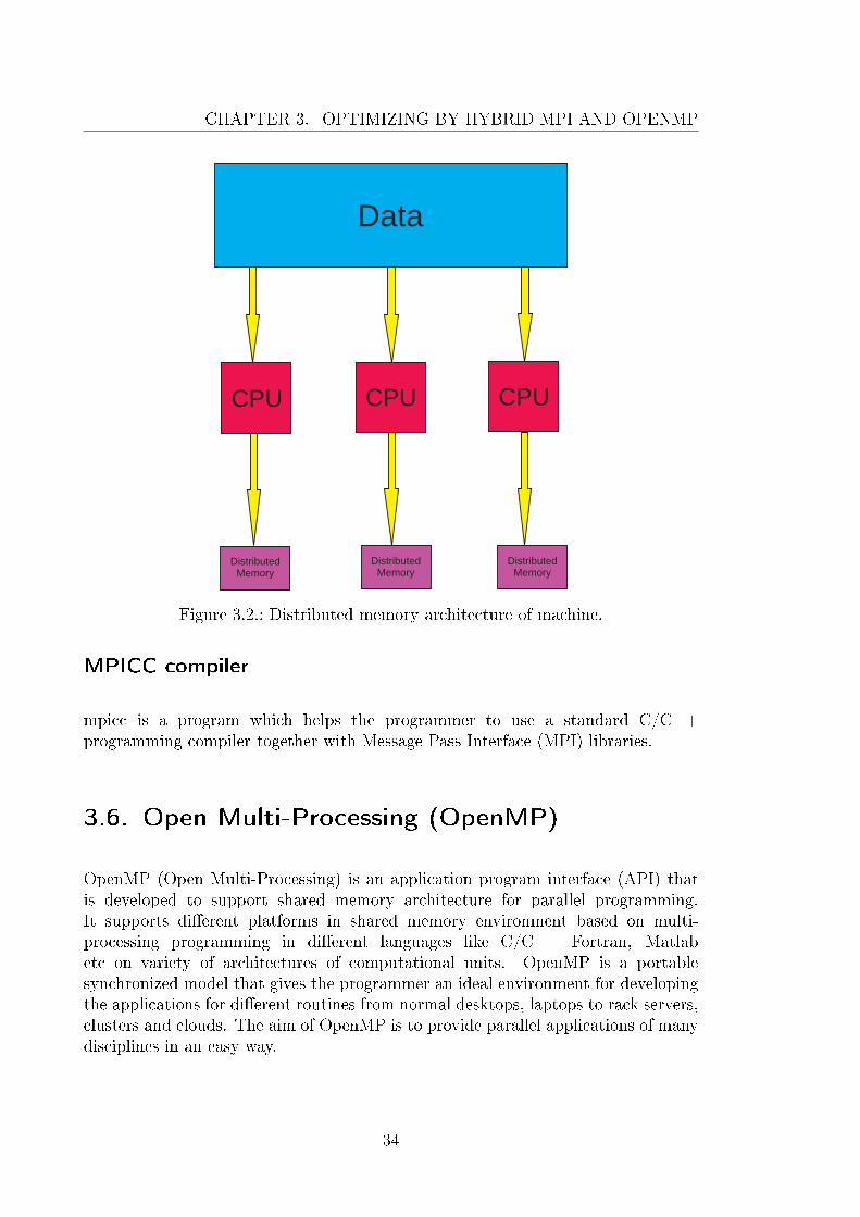
The MPI interface is meant to provide a synchronized path and optimizedcommunication between the set of processes, which are directed to nodes, clusters,servers or computers independent of the language in which the task is programmed.Optimally for high performance, while using MPI, every single core or node shouldbe assigned di�erent independent tasks. For MPI tasks to be performed in a code,a library known as �mpi.h� needs to be included in the header when MPI routinesare called in the program. MPI multi threading follows the distributed memoryarchitecture as shown in Figure 3.2. The �gure illustrates the general idea of thedistributed memory architecture in which each CPU or node is assigned the speci�camount of memory known to be RAM which is used during the multi-tasking. Thedata processed by each CPU is dealed on its speci�c assigned memory part. EachCPU or node is connected with separate physical memory where the data comesand tasks are performed. Node is the group of di�erent CPUs e.g., 8/16/32.
33
CHAPTER 3. OPTIMIZING BY HYBRID MPI AND OPENMP
Data
CPU CPUCPU
DistributedMemory
DistributedMemory
DistributedMemory
DistributedMemory
Figure 3.2.: Distributed memory architecture of machine.
MPICC compiler
mpicc is a program which helps the programmer to use a standard C/C++programming compiler together with Message Pass Interface (MPI) libraries.
3.6. Open Multi-Processing (OpenMP)
OpenMP (Open Multi-Processing) is an application program interface (API) thatis developed to support shared memory architecture for parallel programming.It supports di�erent platforms in shared memory environment based on multi-processing programming in di�erent languages like C/C++ Fortran, Matlabetc on variety of architectures of computational units. OpenMP is a portablesynchronized model that gives the programmer an ideal environment for developingthe applications for di�erent routines from normal desktops, laptops to rack servers,clusters and clouds. The aim of OpenMP is to provide parallel applications of manydisciplines in an easy way.
34
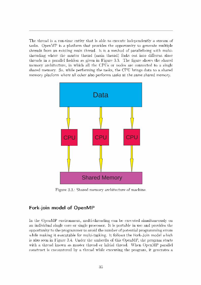
The thread is a run-time entity that is able to execute independently a stream oftasks. OpenMP is a platform that provides the opportunity to generate multiplethreads from an existing main thread. It is a method of parallelizing with multi-threading where the master thread (main thread) forks out into di�erent slavethreads in a parallel fashion as given in Figure 3.3. The �gure shows the sharedmemory architecture, in which all the CPUs or nodes are connected to a singleshared memory. So, while performing the tasks, the CPU brings data to a sharedmemory platform where all other also performs tasks at the same shared memory.
Data
CPU
Shared Memory
CPUCPU
Figure 3.3.: Shared memory architecture of machine.
Fork-join model of OpenMP
In the OpenMP environment, multi-threading can be executed simultaneously onan individual single core or single processor. It is portable in use and provides theopportunity to the programmer to avoid the number of potential programming errorswhile making it executable for multi-tasking. It follows the Fork-Join model whichis also seen in Figure 3.4. Under the umbrella of this OpenMP, the program startswith a thread known as master thread or initial thread. When OpenMP parallelconstruct is encountered by a thread while executing the program, it generates a
35
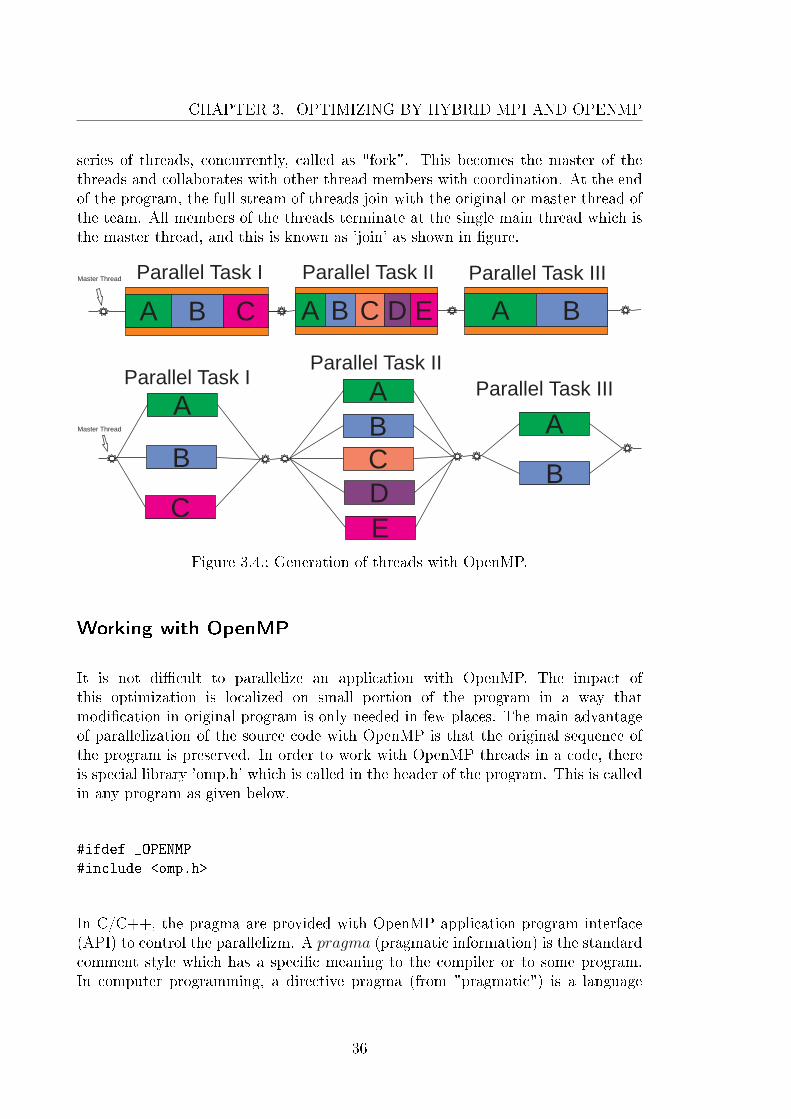
CHAPTER 3. OPTIMIZING BY HYBRID MPI AND OPENMP
series of threads, concurrently, called as "fork". This becomes the master of thethreads and collaborates with other thread members with coordination. At the endof the program, the full stream of threads join with the original or master thread ofthe team. All members of the threads terminate at the single main thread which isthe master thread, and this is known as 'join' as shown in �gure.
B
A
C
D EA B C A B C
A
B
C
D
E
A
B
A
B
Parallel Task I Parallel Task II Parallel Task III
Parallel Task IParallel Task II
Parallel Task III
Master Thread
Master Thread
Figure 3.4.: Generation of threads with OpenMP.
Working with OpenMP
It is not di�cult to parallelize an application with OpenMP. The impact ofthis optimization is localized on small portion of the program in a way thatmodi�cation in original program is only needed in few places. The main advantageof parallelization of the source code with OpenMP is that the original sequence ofthe program is preserved. In order to work with OpenMP threads in a code, thereis special library 'omp.h' which is called in the header of the program. This is calledin any program as given below.
#ifdef _OPENMP
#include <omp.h>
In C/C++, the pragma are provided with OpenMP application program interface(API) to control the parallelizm. A pragma (pragmatic information) is the standardcomment style which has a speci�c meaning to the compiler or to some program.In computer programming, a directive pragma (from "pragmatic") is a language
36

construct that speci�es how a compiler (or assembler or interpreter) should processits input. Directives are not part of the language, they are not part of the grammar,and may vary from compiler to compiler, but instead function either as an in-bandform of a command-line option, specifying compiler behaviour, or are processed bya preprocessor. In OpenMP, these (pragmas) are called compiler directives. Theystart with #pragma omp followed by the key to identify the directive. A largenumber of applications can be parallelized by using few compiler constructs or oneor more functions like :
� Parallel construct
� Work-load sharing construct
These constructs decide what should be done by parallelization of task (Chapmanet al., 2008). Suppose if a programmer has to generate some threads at some taskinside the program, then the programmer has to instruct to initialize some parallelthreads. It is not di�cult to handle this situation, as a programmer can easilycontrol the threading during programming. The threads depend on demand, eithercan be maximum possible, or one can de�ne the number of threads to generate atthe task level. For a small program it can be done like :
#pragma omp paralel
{
printf("CRS_Express %d\n",
omp_get_num_thread());
}
} /* -- End of Parallel route --*/
The important point is that if the speci�c task in a code is executed in parallelfashion, then the parallel construct should be closed at the end when that task iscompleted.
3.7. Hybrid approach for optimizing
common-re�ection-surface-stack (3D CRS)
In a hybrid approach, OpenMP is used together with a MPI implementation toaccelerate the processes. The accelerated version of the hybrid 3D CRS is named asCRS express.
37
CHAPTER 3. OPTIMIZING BY HYBRID MPI AND OPENMP
The original 3D common-re�ection-surface-stacking (CRS) code by Müller for 3Dvolumes takes a lot of time in processing. Almost 94 % of the time is consumed incalculating the semblance during the search process. The idea is to accelerate thecomputational process in terms of time with same available resources and with thesame output. Addition of concurrent programming at some routines and OpenMPare incorporated in the MPI based 3D CRS code. This optimization is done in someroutines without changing the actual structure of the code. At some parts, parallelthreads have been generated to optimize the tasking in parallel fashion. This isan easy task to implement. The process is robust and works better while utilizingall available resources of the machine. It is more e�cient in the shared memoryarchitecture compared to parallel memory based units. Some initial tests show that,the processing is 10 times faster then the original 3D CRS code in terms of e�ciency.The observed progress is shown in Figure 3.5. In ideal conditions, when libraries aremore suited for compiling the program, the code works even more than ten timesfaster then the original version as shown in the graph.
Test analysis of hybrid implementation
In order to check whether this implementation is successful and perfectly workingfor the seismic data processing, some initial tests have been performed on syntheticdata set. For this, 2D Sigsbee 2A seismic data has been used to compare results ofthe original code with the hybrid CRS express code. In this test, not only the timecomparison has been checked, also the quality of the output of the seismic datasethas been observed in detail.
3.8. Practical application (Synthetic data
example)
For analysis of the hybrid CRS, di�erent tests have been performed �rst onsynthetic dataset. For this purpose, 2D Sigsbee 2A has been used to check thereliability of the performance of the code and the quality of the output.
Sigsbee 2A is a synthetic 2D dataset consisting of a single seismic pro�le. This isa marine dataset with a complex sub-surface salt body and some di�ractions. Forcomparison, this dataset is also reliable to investigate the re�ections and di�ractionsresponse. Although this is a 2D dataset, the code can handle both types of dataset(2D and 3D) for processing. The main reason of testing the hybrid 3D CRS code
38

0 50 100 150 200 2500
5
10
15
20
No of cores
Rela
tive a
ccele
ration
Figure 3.5.: Graph showing the 3D CRS (express) processing with time.(relative acceleration of the hybridized MPI+OpenMP 3D CRSimplementation as a function of number of cores)
on Sigsbee 2A dataset is that, this is a well known dataset and if there is any �awor defect in the output, then it could be easily detected.
For test analysis, the complete procedure of CRS stacking was performed with theCRS express code to check the attribute calculations and parameter estimations,and to test whether it works similar to the original code. Both codes are testedon the same machine, on the same dataset, on same the number of cores with thesame parameters. The process of CRS is performed in sequence. The resultingoutput shows that the attributes computed by the hybrid code are the same as theattributes computed with the original code. The resulting cpu time is at least 10times faster then that of the original code.
39
CHAPTER 3. OPTIMIZING BY HYBRID MPI AND OPENMP
If we compare the CMP stack of the original code with the hybrid code, we cannotdistinguish noticeable di�erence in the output in Figure 3.6 and Figure 3.7 . Themost important point is to have a similar output of the attributes. So, whilecomparing the di�erence between the output of the original and hybrid CRS code, acloser look is done for di�erent attributes. Starting from the Figure 3.8 and Figure3.9 which show the radius of curvature of normal incidence point wave. Both in thisplan shown the same output result. The other main attribute is the angle which isin Figure 3.10 and Figure 3.11. Here in these two �gures, we see that there is nodi�erence at all in terms of re�ections and di�ractions. Similar conclusions applyfor other attributes like curvature of normal wave in Figure 3.12 and Figure 3.13.
One of the outputs provided by this code is the coherence which is an importantingredient of the CRS work�ow. If we compare the coherence of the originalcode in Figure 3.14 versus the (later used) hybrid optimized code in Figure 3.15,then both are same and there is no di�erence in the output section of either of them.
The last comparison is in the �nal output the CRS stacked section. Figure 3.16 andFigure 3.17 gives a clear indication that both results look similar. So, this meansthat the output of the CRS stack with its attributes is same in the hybrid optimizedoutput compared to the original code. Direct comparison of the results of outputfrom both codes (original and hybrid) show very little or almost negligible di�erencein output.
3.9. Discussion and conclusion
In this hybrid optimization, the important target was to accelerate the code in orderto be able to work on a bigger scale. The whole e�ort to work on the accelerationis to optimize the code so that it should be able to deal with the industrial scaledataset in an academic environment on the small computers. The results in outputshows that the optimized output is not only similar compared to the original code,but its computational cost is 10 times less. For big Tera-byte dataset, this e�orthelps to get the results by saving several days of CPU time.
40
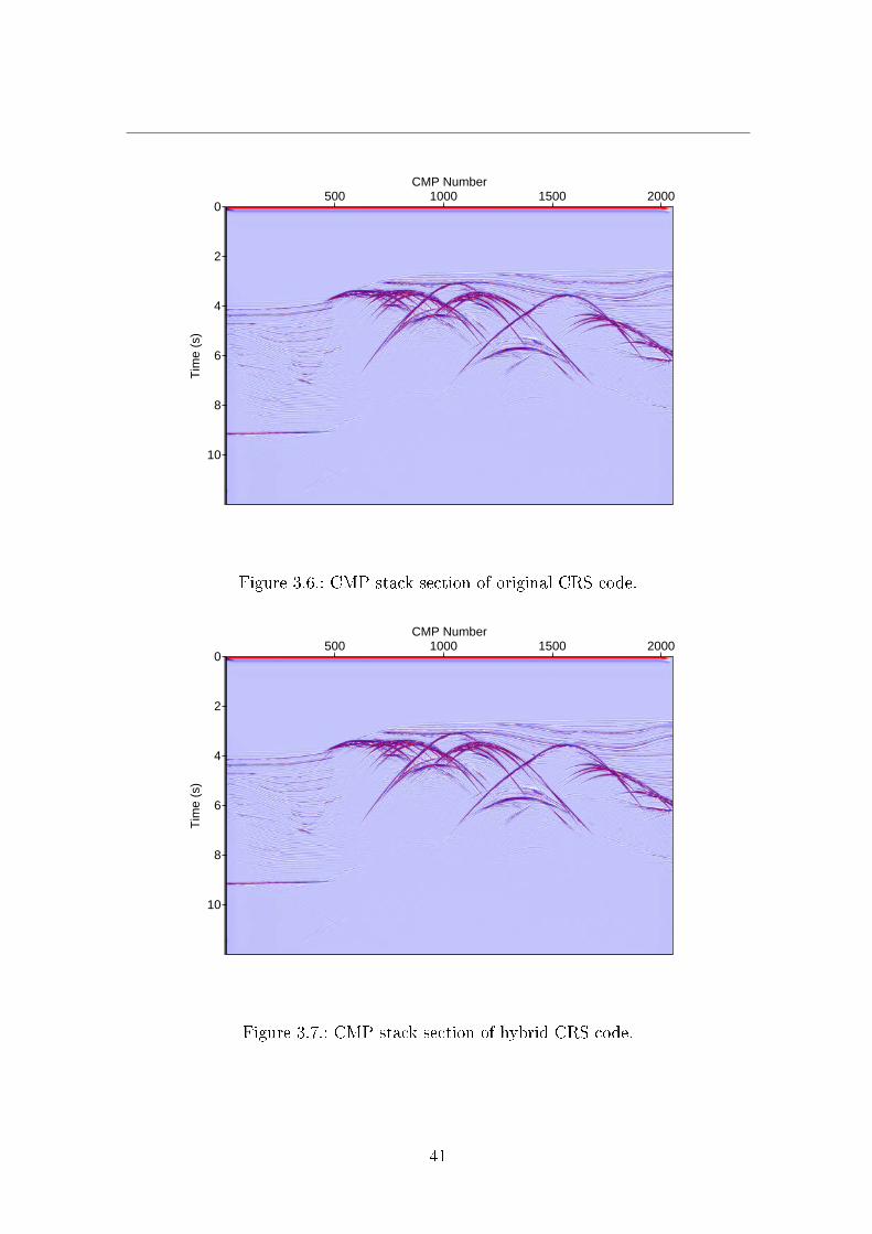
0
2
4
6
8
10
Tim
e (
s)
500 1000 1500 2000CMP Number
Figure 3.6.: CMP stack section of original CRS code.
0
2
4
6
8
10
Tim
e (
s)
500 1000 1500 2000CMP Number
Figure 3.7.: CMP stack section of hybrid CRS code.
41
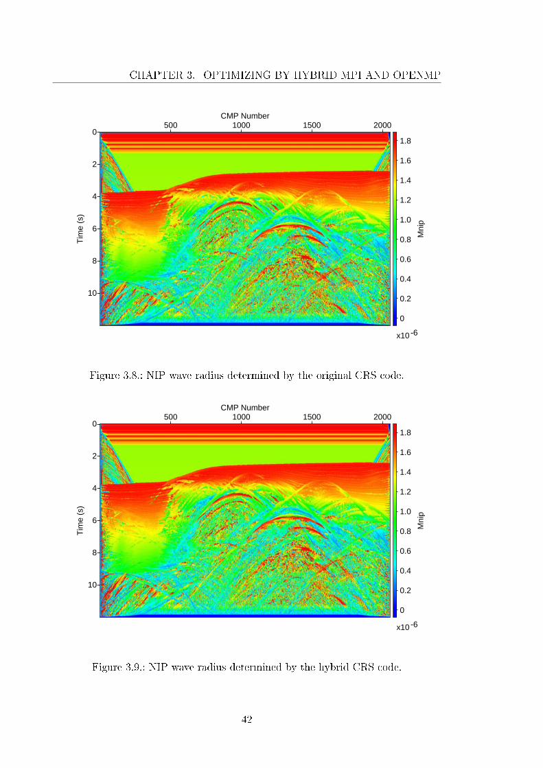
CHAPTER 3. OPTIMIZING BY HYBRID MPI AND OPENMP
0
2
4
6
8
10
Tim
e (
s)
500 1000 1500 2000CMP Number
0
0.2
0.4
0.6
0.8
1.0
1.2
1.4
1.6
1.8
x10 -6
Mnip
Figure 3.8.: NIP wave radius determined by the original CRS code.
0
2
4
6
8
10
Tim
e (
s)
500 1000 1500 2000CMP Number
0
0.2
0.4
0.6
0.8
1.0
1.2
1.4
1.6
1.8
x10 -6
Mnip
Figure 3.9.: NIP wave radius determined by the hybrid CRS code.
42
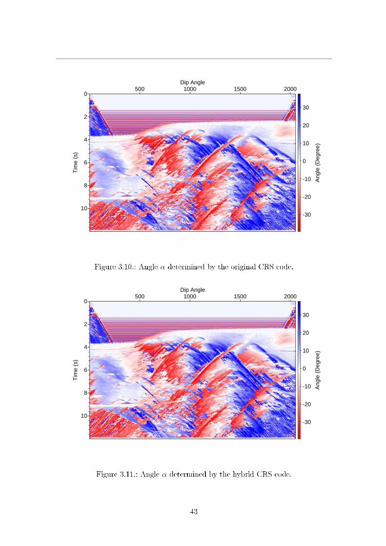
0
2
4
6
8
10
Tim
e (
s)
500 1000 1500 2000Dip Angle
-30
-20
-10
0
10
20
30
Angle
(D
egre
e)
Figure 3.10.: Angle α determined by the original CRS code.
0
2
4
6
8
10
Tim
e (
s)
500 1000 1500 2000Dip Angle
-30
-20
-10
0
10
20
30A
ngle
(D
egre
e)
Figure 3.11.: Angle α determined by the hybrid CRS code.
43

CHAPTER 3. OPTIMIZING BY HYBRID MPI AND OPENMP
0
2
4
6
8
10
Tim
e (
s)
500 1000 1500 2000CMP Number
-1.0
-0.8
-0.6
-0.4
-0.2
0
0.2
0.4
0.6
0.8
1.0
x10 -6
Mn
Figure 3.12.: N wave curvature determined by the original CRS code.
0
2
4
6
8
10
Tim
e (
s)
500 1000 1500 2000CMP Number
-1.0
-0.8
-0.6
-0.4
-0.2
0
0.2
0.4
0.6
0.8
1.0
x10 -6
Mn
Figure 3.13.: N wave curvature determined by the hybrid CRS code.
44
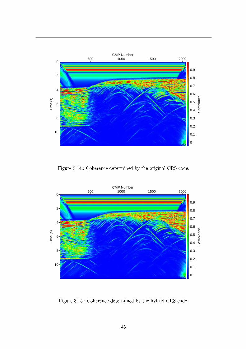
0
2
4
6
8
10
Tim
e (
s)
500 1000 1500 2000CMP Number
0
0.1
0.2
0.3
0.4
0.5
0.6
0.7
0.8
0.9
Sem
bla
nce
Figure 3.14.: Coherence determined by the original CRS code.
0
2
4
6
8
10
Tim
e (
s)
500 1000 1500 2000CMP Number
0
0.1
0.2
0.3
0.4
0.5
0.6
0.7
0.8
0.9S
em
bla
nce
Figure 3.15.: Coherence determined by the hybrid CRS code.
45

CHAPTER 3. OPTIMIZING BY HYBRID MPI AND OPENMP
0
2
4
6
8
10
Tim
e (
s)
500 1000 1500 2000CMP Number
Figure 3.16.: CRS stack section obtained by the original CRS code.
0
2
4
6
8
10
Tim
e (
s)
500 1000 1500 2000CMP Number
Figure 3.17.: CRS stack section obtained by the hybrid CRS code.
46
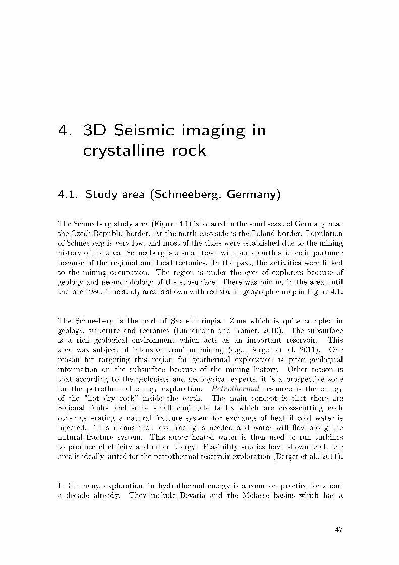
4. 3D Seismic imaging in
crystalline rock
4.1. Study area (Schneeberg, Germany)
The Schneeberg study area (Figure 4.1) is located in the south-east of Germany nearthe Czech Republic border. At the north-east side is the Poland border. Populationof Schneeberg is very low, and most of the cities were established due to the mininghistory of the area. Schneeberg is a small town with some earth science importancebecause of the regional and local tectonics. In the past, the activities were linkedto the mining occupation. The region is under the eyes of explorers because ofgeology and geomorphology of the subsurface. There was mining in the area untilthe late 1980. The study area is shown with red star in geographic map in Figure 4.1.
The Schneeberg is the part of Saxo-thuringian Zone which is quite complex ingeology, structure and tectonics (Linnemann and Romer, 2010). The subsurfaceis a rich geological environment which acts as an important reservoir. Thisarea was subject of intensive uranium mining (e.g., Berger et al. 2011). Onereason for targeting this region for geothermal exploration is prior geologicalinformation on the subsurface because of the mining history. Other reason isthat according to the geologists and geophysical experts, it is a prospective zonefor the petrothermal energy exploration. Petrothermal resource is the energyof the "hot dry rock" inside the earth. The main concept is that there areregional faults and some small conjugate faults which are cross-cutting eachother generating a natural fracture system for exchange of heat if cold water isinjected. This means that less fracing is needed and water will �ow along thenatural fracture system. This super heated water is then used to run turbinesto produce electricity and other energy. Feasibility studies have shown that, thearea is ideally suited for the petrothermal reservoir exploration (Berger et al., 2011).
In Germany, exploration for hydrothermal energy is a common practice for abouta decade already. They include Bevaria and the Molasse basins which has a
47
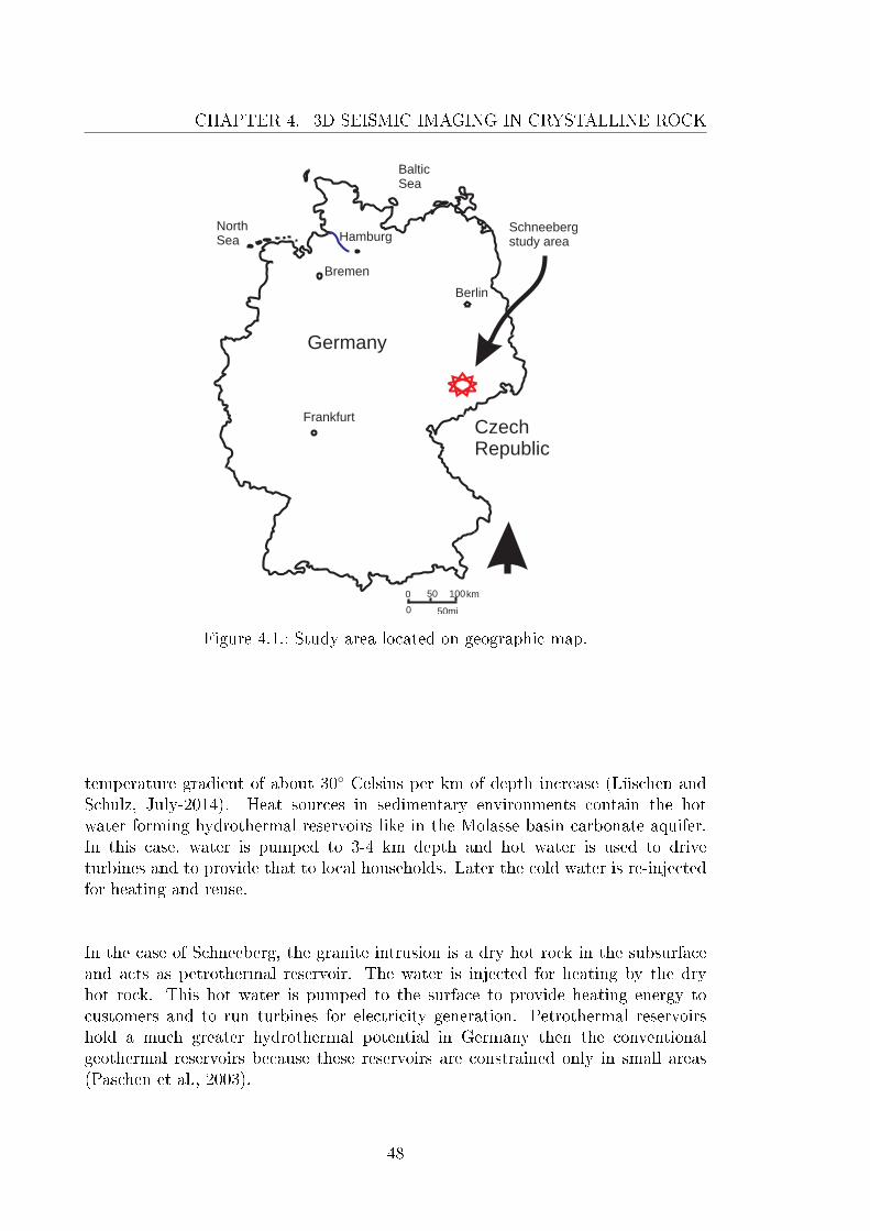
CHAPTER 4. 3D SEISMIC IMAGING IN CRYSTALLINE ROCK
Frankfurt
Hamburg
Berlin
Germany
CzechRepublic
NorthSea
BalticSea
0 50 100
50mi
km
0
Schneebergstudy area
Bremen
Figure 4.1.: Study area located on geographic map.
temperature gradient of about 30◦ Celsius per km of depth increase (Lüschen andSchulz, July-2014). Heat sources in sedimentary environments contain the hotwater forming hydrothermal reservoirs like in the Molasse basin carbonate aquifer.In this case, water is pumped to 3-4 km depth and hot water is used to driveturbines and to provide that to local households. Later the cold water is re-injectedfor heating and reuse.
In the case of Schneeberg, the granite intrusion is a dry hot rock in the subsurfaceand acts as petrothermal reservoir. The water is injected for heating by the dryhot rock. This hot water is pumped to the surface to provide heating energy tocustomers and to run turbines for electricity generation. Petrothermal reservoirshold a much greater hydrothermal potential in Germany then the conventionalgeothermal reservoirs because these reservoirs are constrained only in small areas(Paschen et al., 2003).
48
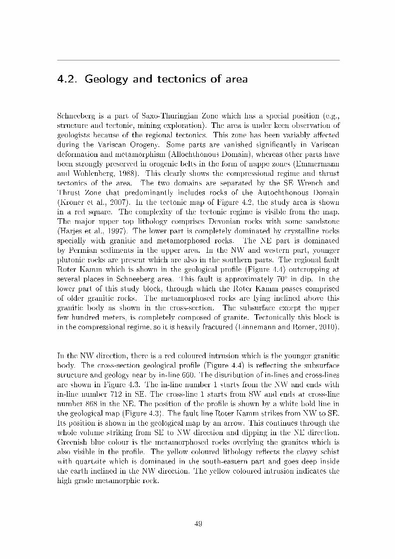
4.2. Geology and tectonics of area
Schneeberg is a part of Saxo-Thuringian Zone which has a special position (e.g.,structure and tectonic, mining exploration). The area is under keen observation ofgeologists because of the regional tectonics. This zone has been variably a�ectedduring the Variscan Orogeny. Some parts are vanished signi�cantly in Variscandeformation and metamorphism (Allochthonous Domain), whereas other parts havebeen strongly preserved in orogenic belts in the form of nappe zones (Emmermannand Wohlenberg, 1988). This clearly shows the compressional regime and thrusttectonics of the area. The two domains are separated by the SE Wrench andThrust Zone that predominantly includes rocks of the Autochthonous Domain(Kroner et al., 2007). In the tectonic map of Figure 4.2, the study area is shownin a red square. The complexity of the tectonic regime is visible from the map.The major upper top lithology comprises Devonian rocks with some sandstone(Harjes et al., 1997). The lower part is completely dominated by crystalline rocksspecially with granitic and metamorphosed rocks. The NE part is dominatedby Permian sediments in the upper area. In the NW and western part, youngerplutonic rocks are present which are also in the southern parts. The regional faultRoter Kamm which is shown in the geological pro�le (Figure 4.4) outcropping atseveral places in Schneeberg area. This fault is approximately 70◦ in dip. In thelower part of this study block, through which the Roter Kamm passes comprisedof older granitic rocks. The metamorphosed rocks are lying inclined above thisgranitic body as shown in the cross-section. The subsurface except the upperfew hundred meters, is completely composed of granite. Tectonically this block isin the compressional regime, so it is heavily fractured (Linnemann and Romer, 2010).
In the NW direction, there is a red coloured intrusion which is the younger graniticbody. The cross-section geological pro�le (Figure 4.4) is re�ecting the subsurfacestructure and geology near by in-line 660. The distribution of in-lines and cross-linesare shown in Figure 4.3. The in-line number 1 starts from the NW and ends within-line number 712 in SE. The cross-line 1 starts from SW and ends at cross-linenumber 868 in the NE. The position of the pro�le is shown by a white bold line inthe geological map (Figure 4.3). The fault line Roter Kamm strikes from NW to SE.Its position is shown in the geological map by an arrow. This continues through thewhole volume striking from SE to NW direction and dipping in the NE direction.Greenish blue colour is the metamorphosed rocks overlying the granites which isalso visible in the pro�le. The yellow coloured lithology re�ects the clayey schistwith quartzite which is dominated in the south-eastern part and goes deep insidethe earth inclined in the NW direction. The yellow coloured intrusion indicates thehigh grade metamorphic rock.
49

CHAPTER 4. 3D SEISMIC IMAGING IN CRYSTALLINE ROCK
High gradeVariscanoverprints
Plutons Suturezone
Cadomainback-arc basin
Passivemargindeposit
Devonianrocks
Variscannappes
Variscanwild flysch
Figure 4.2.: Regional tectonic map showing Schneeberg study area (Linnemann andRomer, 2010).
Conjugate faults are present dipping perpendicular to the Roter Kamm as shown ingeological cross-section. The inclined overlying layers of rocks are metamorphosedrocks which are present on top of the granitic body. The conjugate faults cross cutthe metamorphic rocks. Conjugate faults terminate at the Roter Kamm.
In this geological map of Schneeberg, there is a brown coloured area in NE part.This area was exposed to mining on a large scale in the past. Still in some partsmining is continued till today.
4.3. Seismic acquisition (Survey design)
In this 3D seismic acquisition, vibroseis is used as the energy source for generatingseismic waves. The study area comprises 140 km2 with northening from 5602955to 5619705 and eastening from 4538275 to 4555025. The planing projection of the
50
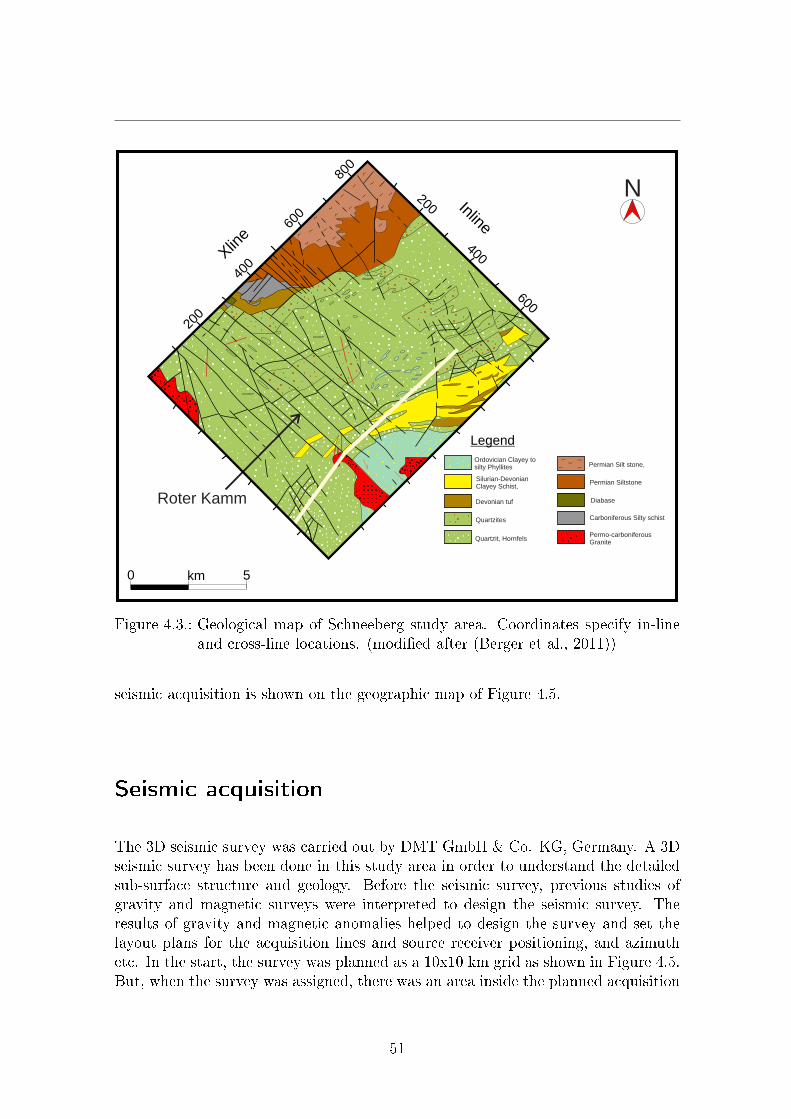
Legend
5km0
Ordovician Clayey tosilty Phyllites
Quartzites
Silurian-DevonianClayey Schist,
Devonian tuf
Quartzit, Hornfels
Permian Silt stone,
Permian Siltstone
Diabase
Permo-carboniferousGranite
Carboniferous Silty schist
Roter Kamm
200N
200
400
600
800
400
600
Inline
Xlin
e
Figure 4.3.: Geological map of Schneeberg study area. Coordinates specify in-lineand cross-line locations. (modi�ed after (Berger et al., 2011))
seismic acquisition is shown on the geographic map of Figure 4.5.
Seismic acquisition
The 3D seismic survey was carried out by DMT GmbH & Co. KG, Germany. A 3Dseismic survey has been done in this study area in order to understand the detailedsub-surface structure and geology. Before the seismic survey, previous studies ofgravity and magnetic surveys were interpreted to design the seismic survey. Theresults of gravity and magnetic anomalies helped to design the survey and set thelayout plans for the acquisition lines and source receiver positioning, and azimuthetc. In the start, the survey was planned as a 10x10 km grid as shown in Figure 4.5.But, when the survey was assigned, there was an area inside the planned acquisition
51

CHAPTER 4. 3D SEISMIC IMAGING IN CRYSTALLINE ROCK
SW NE
LEGEND
S-D
O -OFr Ph
FaultsOrdovician SilurianDevonian rock
OrdovicianQuartzite
Phyllites
Ordovician PhyllitesDiabase Quartzite
Older granite with eruptive complexand mirror stone like rock
Y
OT3
Roter K
amm
OT3
O -OFr PhO
T3
S-D
Y
0
1
2
3
4
(km)2 km
Figure 4.4.: Cross-section of Schneeberg study area passing near in-line 660. (Bergeret al., 2011)
grid, which was not permitted to be surveyed by authorities. Due to this reason,the survey plan was changed and extended from 10 km to 13.5 km in the north-eastern part. The non-permitted area is shown in Figure 4.6 as a purple patch.This does not allow continuous coverage of the seismic survey. The acquisition teamhad to plan the extension of the grid for the seismic survey to obtain the maximumpossible coverage of the subsurface signal in the area of interest. The extended newsurvey plan is shown in Figure 4.6. DMT has done the acquisition of this area. Theacquisition was done with the azimuth of 45◦ from North. The data acquisition wascompleted in November, 2012. The fold density map is shown in the Figure 4.7
52
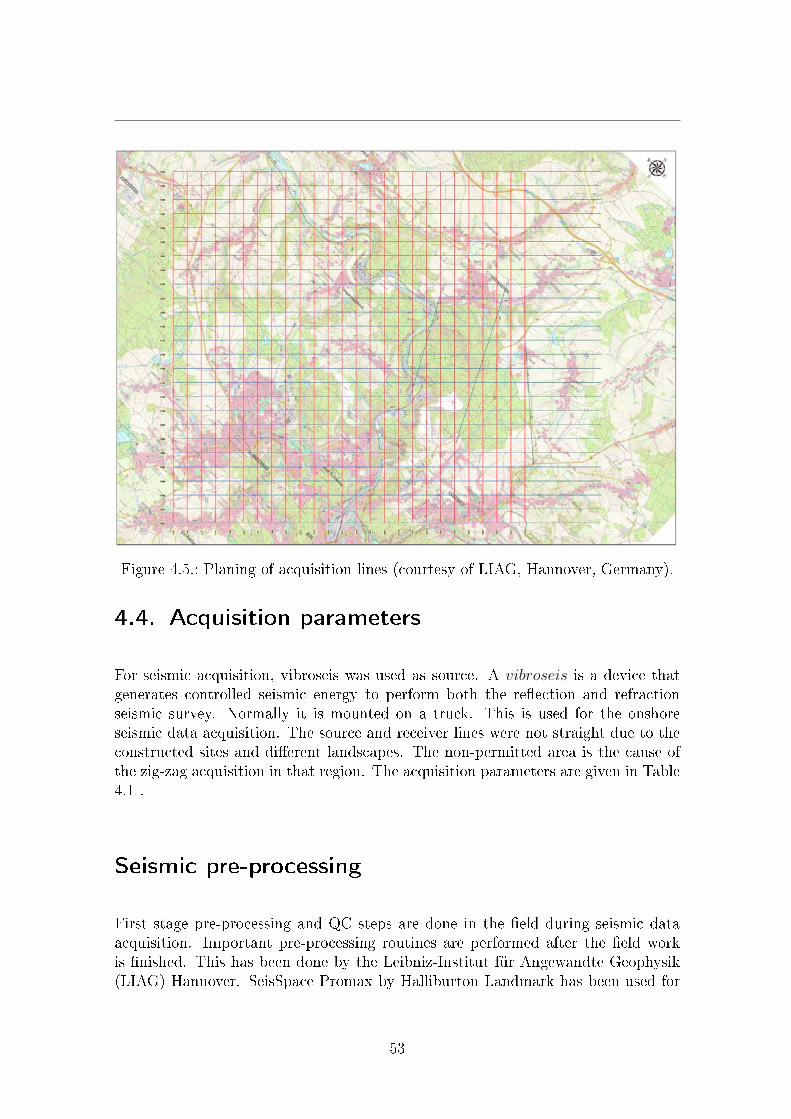
Figure 4.5.: Planing of acquisition lines (courtesy of LIAG, Hannover, Germany).
4.4. Acquisition parameters
For seismic acquisition, vibroseis was used as source. A vibroseis is a device thatgenerates controlled seismic energy to perform both the re�ection and refractionseismic survey. Normally it is mounted on a truck. This is used for the onshoreseismic data acquisition. The source and receiver lines were not straight due to theconstructed sites and di�erent landscapes. The non-permitted area is the cause ofthe zig-zag acquisition in that region. The acquisition parameters are given in Table4.1 .
Seismic pre-processing
First stage pre-processing and QC steps are done in the �eld during seismic dataacquisition. Important pre-processing routines are performed after the �eld workis �nished. This has been done by the Leibniz-Institut für Angewandte Geophysik(LIAG) Hannover. SeisSpace Promax by Halliburton Landmark has been used for
53

CHAPTER 4. 3D SEISMIC IMAGING IN CRYSTALLINE ROCK
Parameter Value / UnitSeismic source VibroseisSweep length 10 secFrequency content 12 Hz - 96 HzGeophone content 1 CAcquisition area volume 140 sq kmRecording time 10 secTime sample rate 2 msNo of channels 6000No of receivers 8146No of source points 5348Source interval 30 mReceiver interval 30 mSource line interval 400 mReceiver line interval 400 mMaximum o�set 14000 mNo of in-lines 712No of cross-lines 868No of CMPs 617651No of traces 31198591Max no of fold 150CMP bin spacing 15 mSpacing between in-lines 15 mSpacing between cross-lines 15 m
Table 4.1.: 3D seismic data acquisition parameters.
54
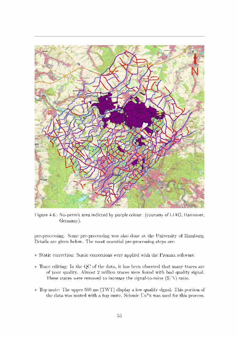
N
Figure 4.6.: No-permit area indicted by purple colour. (courtesy of LIAG, Hannover,Germany).
pre-processing. Some pre-processing was also done at the University of Hamburg.Details are given below. The most essential pre-processing steps are:
∗ Static correction: Static corrections were applied with the Promax software.
∗ Trace editing: In the QC of the data, it has been observed that many traces areof poor quality. Almost 2 million traces were found with bad quality signal.These traces were removed to increase the signal-to-noise (S/N) ratio.
∗ Top mute: The upper 500 ms (TWT) display a low quality signal. This portion ofthe data was muted with a top mute. Seismic Un*x was used for this process.
55
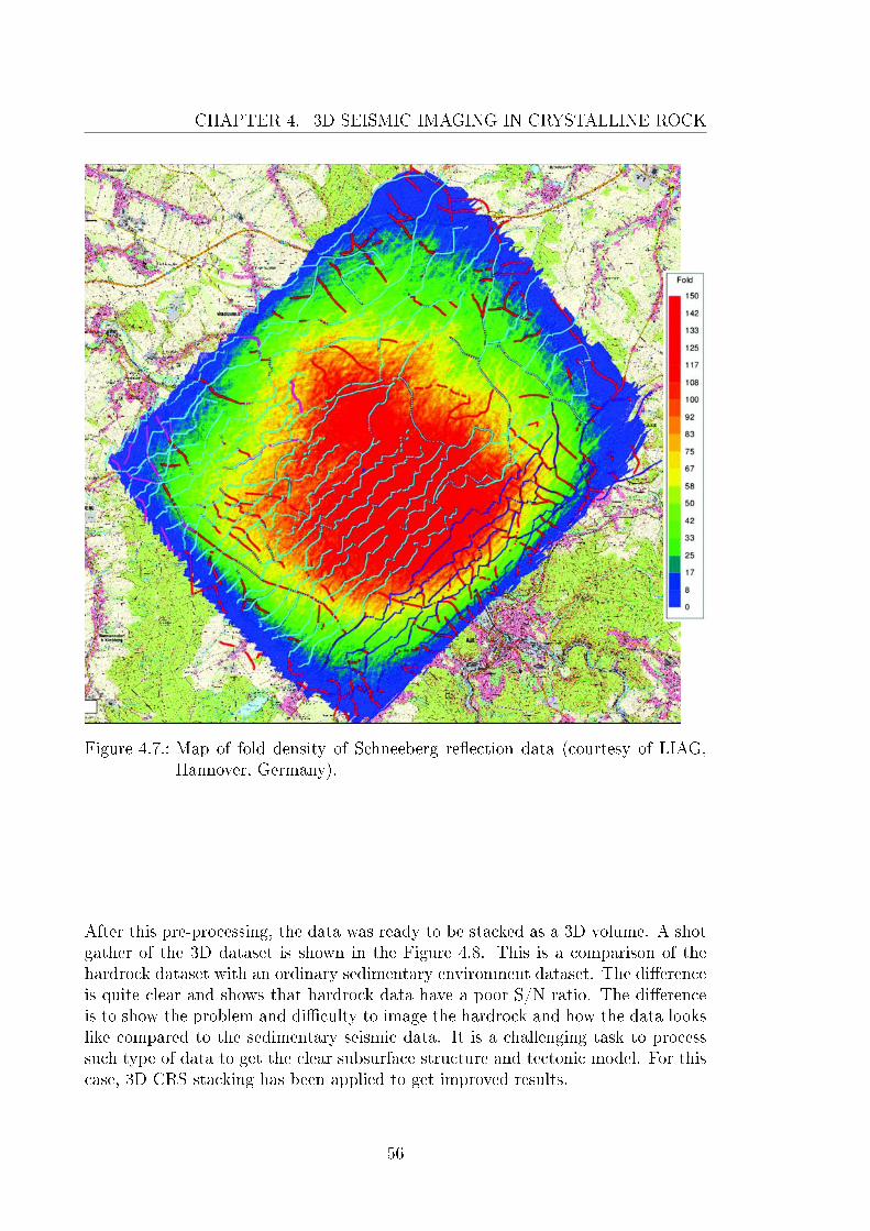
CHAPTER 4. 3D SEISMIC IMAGING IN CRYSTALLINE ROCK
Figure 4.7.: Map of fold density of Schneeberg re�ection data (courtesy of LIAG,Hannover, Germany).
After this pre-processing, the data was ready to be stacked as a 3D volume. A shotgather of the 3D dataset is shown in the Figure 4.8. This is a comparison of thehardrock dataset with an ordinary sedimentary environment dataset. The di�erenceis quite clear and shows that hardrock data have a poor S/N ratio. The di�erenceis to show the problem and di�culty to image the hardrock and how the data lookslike compared to the sedimentary seismic data. It is a challenging task to processsuch type of data to get the clear subsurface structure and tectonic model. For thiscase, 3D CRS stacking has been applied to get improved results.
56
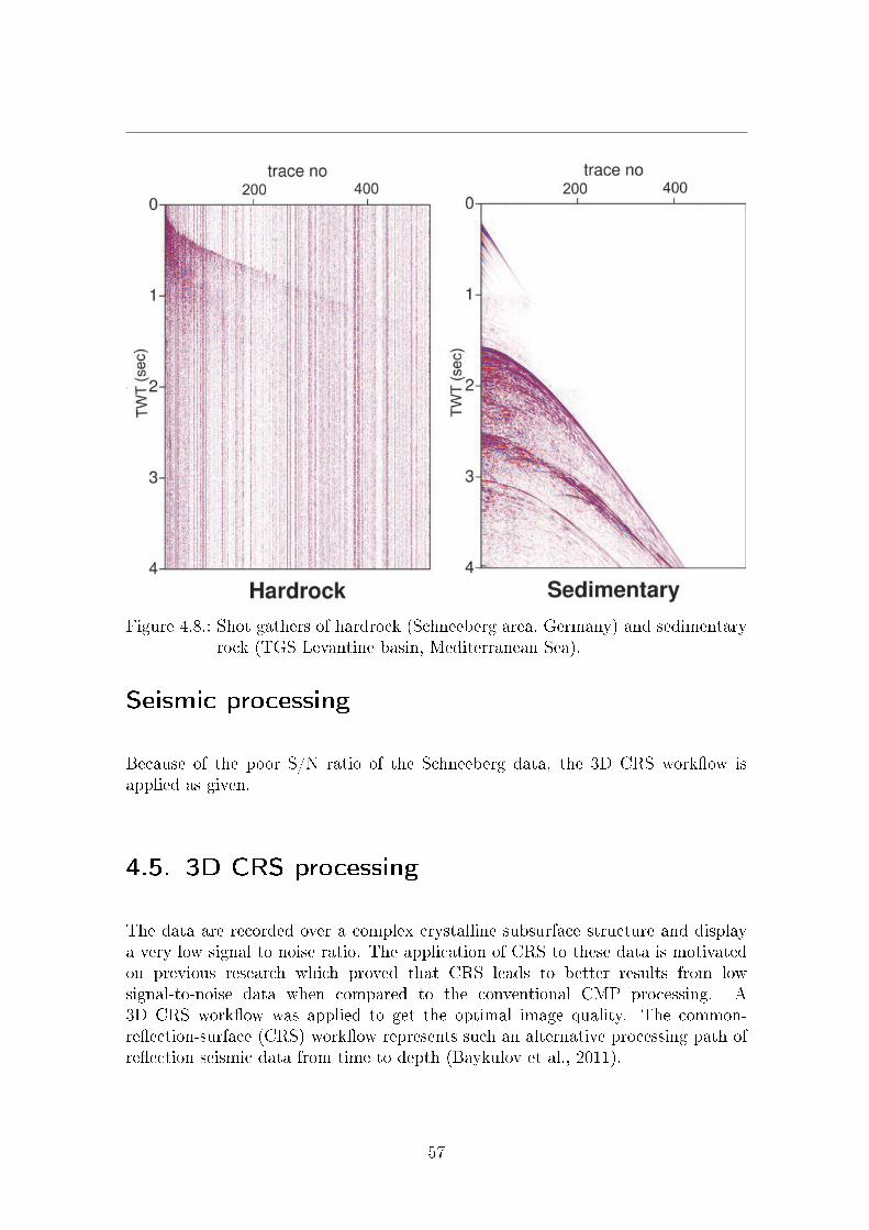
Figure 4.8.: Shot gathers of hardrock (Schneeberg area, Germany) and sedimentaryrock (TGS Levantine basin, Mediterranean Sea).
Seismic processing
Because of the poor S/N ratio of the Schneeberg data, the 3D CRS work�ow isapplied as given.
4.5. 3D CRS processing
The data are recorded over a complex crystalline subsurface structure and displaya very low signal to noise ratio. The application of CRS to these data is motivatedon previous research which proved that CRS leads to better results from lowsignal-to-noise data when compared to the conventional CMP processing. A3D CRS work�ow was applied to get the optimal image quality. The common-re�ection-surface (CRS) work�ow represents such an alternative processing path ofre�ection seismic data from time to depth (Baykulov et al., 2011).
57
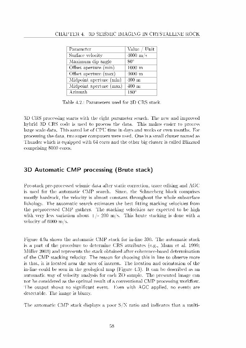
CHAPTER 4. 3D SEISMIC IMAGING IN CRYSTALLINE ROCK
Parameter Value / UnitSurface velocity 4000 m/sMaximum dip angle 80◦
O�set aperture (min) 1000 mO�set aperture (max) 4000 mMidpoint aperture (min) 400 mMidpoint aperture (max) 400 mAzimuth 180◦
Table 4.2.: Parameters used for 3D CRS stack.
3D CRS processing starts with the eight parameter search. The new and improvedhybrid 3D CRS code is used to process the data. This makes easier to processlarge scale data. This saved lot of CPU time in days and weeks or even months. Forprocessing the data, two super computers were used. One is a small cluster named asThunder which is equipped with 64 cores and the other big cluster is called Blizzardcomprising 8000 cores.
3D Automatic CMP processing (Brute stack)
Pre-stack pre-processed seismic data after static correction, trace editing and AGCis used for the automatic CMP search. Since, the Schneeberg block comprisesmostly hardrock, the velocity is almost constant throughout the whole subsurfacelithology. The automatic search estimates the best �tting stacking velocities fromthe preprocessed CMP gathers. The stacking velocities are expected to be highwith very less variation about +/- 200 m/s. This brute stacking is done with avelocity of 6000 m/s.
Figure 4.9a shows the automatic CMP stack for in-line 390. The automatic stackis a part of the procedure to determine CRS attributes (e.g., Mann et al. 1999;Müller 2003) and represents the stack obtained after coherence-based determinationof the CMP stacking velocity. The reason for choosing this in-line to observe moreis that, it is located near the area of interest. The location and orientation of thein-line could be seen in the geological map (Figure 4.3). It can be described as anautomatic way of velocity analysis for each ZO sample. The presented image cannot be considered as the optimal result of a conventional CMP processing work�ow.The output shows no signi�cant event. Even with AGC applied, no events aredetectable. The image is blurry.
The automatic CMP stack displays a poor S/N ratio and indicates that a multi-
58
parameter stacking method like 3D CRS involves more traces in the stack than theCMP method might provide an improved image. This was our motivation to applythe data-driven CRS work�ow to the Schneeberg hardrock re�ection data.
3D CRS Stacking
After automatic CMP stack, the angle and curvature of normal wave is calculated.This completes the 8 parameters attribute search. In this processsing, the anglesearch is performed in a wide range azimuth directions. The parameters for the 3DCRS search are listed in the Table 4.2.
It is well known that stacks represent an image and are the �rst step on the wayto construct a geological model. It is, however, the only imaging result which isobtained in a purely data-driven fashion, free from any interpretation. In Figure4.9b the CRS stack of in-line 390 is shown. Here re�ection events are clearer,more continuous and easier to distinguish in comparison to the automatic CMPstack in Figure 4.9a. Note, that the color amplitude scales are not the same forboth plots, since the CRS stack has higher amplitudes and dynamic range thanthe CMP stack. Many more traces contribute to the CRS image. Although thequality of the CRS-stacked section is already satisfactory because of the increasedS/N ratio, we also considered the coherence as an additional imaging attribute. Asmentioned above, this attribute is obtained in an objective data-driven way duringthe optimization procedure.
The coherence represents a low-pass positive de�nite version of the ZO stack image.It should display features very similar to the stack but with a decreased resolution.The coherence image of in-line 390 is shown in Figure 4.9c. Note again that, thecolor scale is di�erent from the CMP and CRS sections in this �gure, since thecoherence is always positive and assumes values between 0 and 1. For data with avery good S/N ratio, the coherence section looks similar to a stacked section whereabsolute amplitudes are considered. For noisy data, however, the coherence sectionis the superior choice, since seismic noise does not stack destructively, if absoluteamplitudes are used. In the coherence section it is obvious that the steep dippingcontinuous events crossing the whole section are of similar relevance as the eventsin the top left corner. This conclusion is not so easily derived from the CRS-stackedsection (Figure 4.9b). Therefore, it is concluded that the coherence provides asuitable imaging attribute for the structural interpretation of this particular set ofhardrock data. The coherence value directly re�ects the physical relevance of thestacked event and may therefore be used as a weight to further decrease the noiselevel in the CRS-stacked section.
59
CHAPTER 4. 3D SEISMIC IMAGING IN CRYSTALLINE ROCK
This weighting is performed in Figure 4.9d by simply multiplying the stackedamplitude with the respective local coherence. The S/N ratio of the weighted stackis considerably improved when compared with the unweighted CRS stack (Figure4.9b). The prominent events present in this section are related to the re�ectionsfrom the top of granite which is metamorphic rocks overlying and which could bethe clayey schists which are present in the SE of the survey area (see geologicalmap in Figure 4.3). Since the emphasize here is the application of the CRS methodto hardrock data and the establishment of a data-driven work�ow using variousimaging attributes, no detailed interpretation of the images is given here.
Figure 4.10 presents the coherence section of in-line 369. The coherence section showmany crossing events typical for hardrock data. Several NE-SW dipping structuresare dominating the left part of the section. Between cross-line coordinates 200 and500, strong events were observed for two-way-times larger than 2 s, which are notpresent elsewhere. This structure was called Schneeberg body. The Schneeberg bodyis a geological feature which represents the scattered energy below Roter Kamm atthe position of xline 200 near 2 s time. On this in-line no obvious evidence of theRoter Kamm can be detected. The surface location of the Roter Kamm is at aboutcross-line coordinate 230 for this in-line section. Events attributable to Roter Kammwere actually only obtained on a few in-line sections. The seismic appearance of theRoter Kamm is characterized by a considerably smaller coherence when comparedwith the coherence of the conjugate faults. Conjugate faults are visible in the Figure4.10 and 3D cube. On most in-lines the presence of the Roter Kamm in the studyarea is not expressed directly by a seismic event but by the fault throw of theconjugated faults or increased attenuation (Lüschen et al. 2015). In contrast to thegeological model derived prior to the seismic experiment, the conjugate faults donot terminate at the Roter Kamm (Figure 4.4) but penetrate through it and extendconsiderably further SW.
4.6. 3D poststack Kircho� time migration
To remove the imaging artifacts in the stacked volume, 3D Kircho� poststack timemigration is applied. Promax/Seisspace is used for this process. The parametersused for migration are given in the Table 4.3. As the data is big, the 3D migration iscomputationally expensive. One reason is that the events to be migrated are steepdipping and which needs large apertures for migration. The migration is done witha constant velocity of 6000 m/s since no signi�cant lateral velocity variations areassumed. The variation in velocity is from 5800 m/s to 6200 m/s which is knownfrom the mining information of the subsurface. The resulting output providesimproved results and events are better focused in the 3D CRS stacked volume. The
60
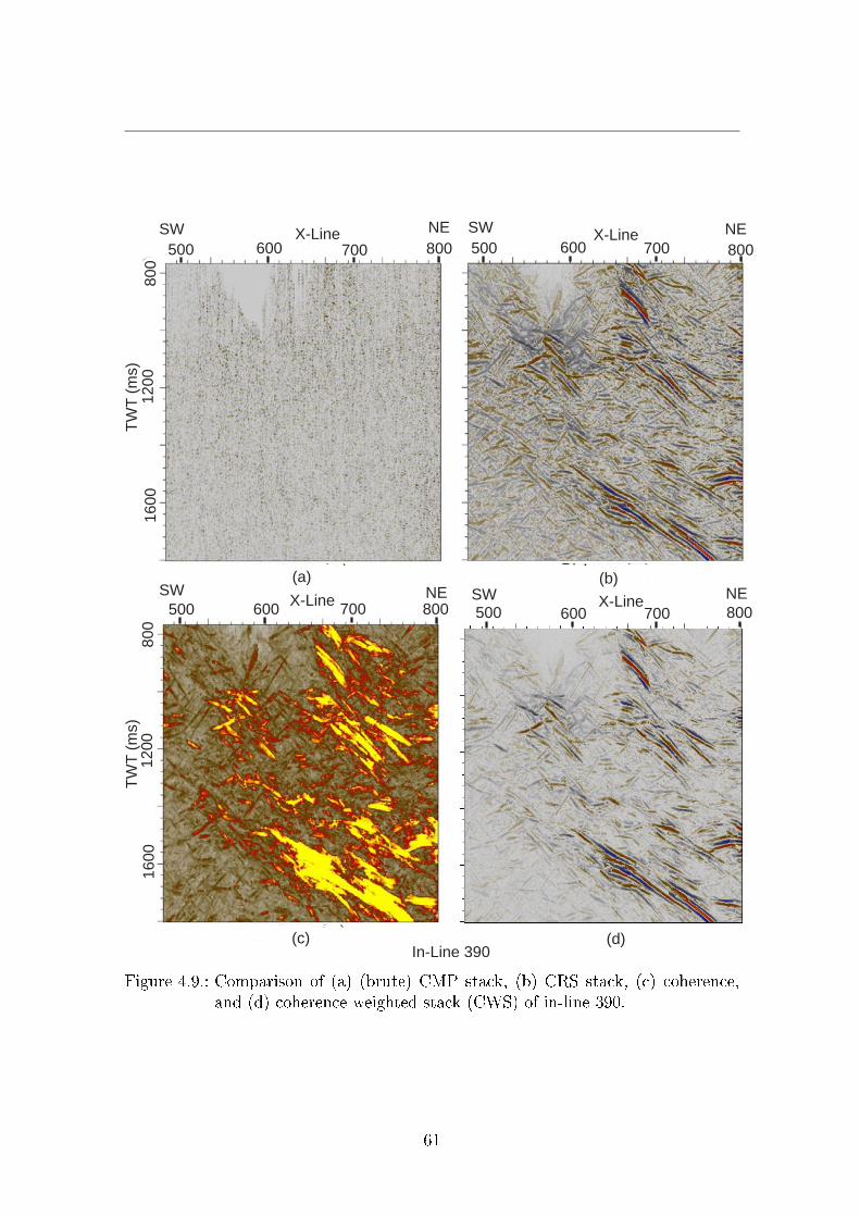
800
1200
1600
TW
T(m
s)
800
1200
TW
T(m
s)
1600
(a) (b)
(d)(c)
500 600 700 800
500 500600 600 700700
800
800800
500 600 700
In-Line 390
SW NE SW NE
SWSW NENEX-Line
X-LineX-Line
X-Line
Figure 4.9.: Comparison of (a) (brute) CMP stack, (b) CRS stack, (c) coherence,and (d) coherence weighted stack (CWS) of in-line 390.
61
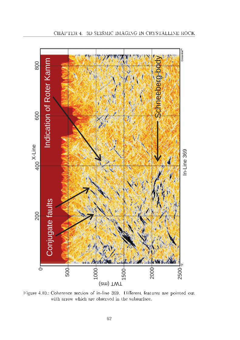
CHAPTER 4. 3D SEISMIC IMAGING IN CRYSTALLINE ROCK200
400
600
800
X-L
ine
In-L
ine 3
69
0
500
1000
1500
2000
2500
TWT(ms)
Sch
ne
eb
erg
bo
dy
Co
nju
ga
te f
au
lts
Ind
ica
tio
n o
f R
ote
r K
am
m
Figure 4.10.: Coherence section of in-line 369. Di�erent features are pointed outwith arrow which are observed in the subsurface.
62
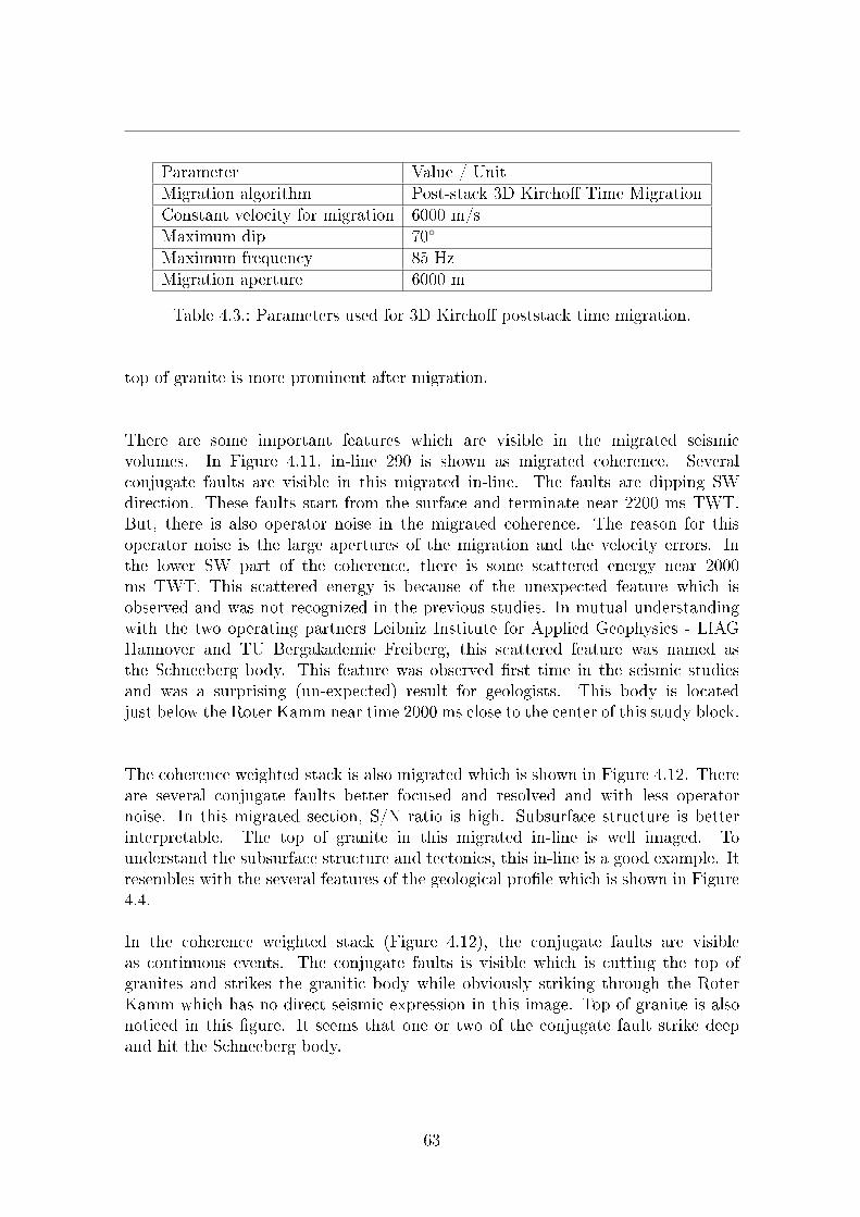
Parameter Value / UnitMigration algorithm Post-stack 3D Kircho� Time MigrationConstant velocity for migration 6000 m/sMaximum dip 70◦
Maximum frequency 85 HzMigration aperture 6000 m
Table 4.3.: Parameters used for 3D Kircho� poststack time migration.
top of granite is more prominent after migration.
There are some important features which are visible in the migrated seismicvolumes. In Figure 4.11, in-line 290 is shown as migrated coherence. Severalconjugate faults are visible in this migrated in-line. The faults are dipping SWdirection. These faults start from the surface and terminate near 2200 ms TWT.But, there is also operator noise in the migrated coherence. The reason for thisoperator noise is the large apertures of the migration and the velocity errors. Inthe lower SW part of the coherence, there is some scattered energy near 2000ms TWT. This scattered energy is because of the unexpected feature which isobserved and was not recognized in the previous studies. In mutual understandingwith the two operating partners Leibniz Institute for Applied Geophysics - LIAGHannover and TU Bergakademie Freiberg, this scattered feature was named asthe Schneeberg body. This feature was observed �rst time in the seismic studiesand was a surprising (un-expected) result for geologists. This body is locatedjust below the Roter Kamm near time 2000 ms close to the center of this study block.
The coherence weighted stack is also migrated which is shown in Figure 4.12. Thereare several conjugate faults better focused and resolved and with less operatornoise. In this migrated section, S/N ratio is high. Subsurface structure is betterinterpretable. The top of granite in this migrated in-line is well imaged. Tounderstand the subsurface structure and tectonics, this in-line is a good example. Itresembles with the several features of the geological pro�le which is shown in Figure4.4.
In the coherence weighted stack (Figure 4.12), the conjugate faults are visibleas continuous events. The conjugate faults is visible which is cutting the top ofgranites and strikes the granitic body while obviously striking through the RoterKamm which has no direct seismic expression in this image. Top of granite is alsonoticed in this �gure. It seems that one or two of the conjugate fault strike deepand hit the Schneeberg body.
63
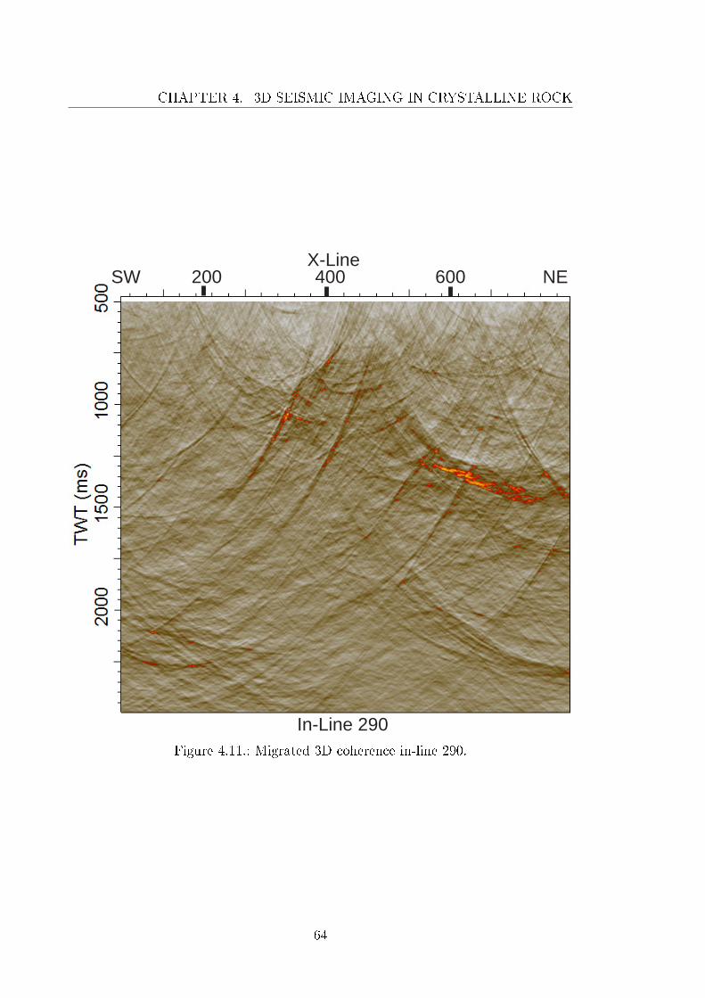
CHAPTER 4. 3D SEISMIC IMAGING IN CRYSTALLINE ROCK
200 400 600
In-Line 290
X-Line
SW NE
Figure 4.11.: Migrated 3D coherence in-line 290.
64

200 400 600
In-Line 290
X-LineSW NE
Figure 4.12.: Migrated coherence weighted CRS stack in-line 290. The features arebetter visible than in coherence.
65
CHAPTER 4. 3D SEISMIC IMAGING IN CRYSTALLINE ROCK
200 400 600
X-line
In-Line 148
SW NE
Figure 4.13.: Migrated 3D coherence weighted CRS stacked in-line 148. Startingfrom below x-line 200, slight hint of Roter Kamm with polarity reversal.
In the detailed study of the migrated stacked, migrated coherence and migratedcoherence weighted stack, di�erent features are visible in di�erent in-lines andcross-lines.
66
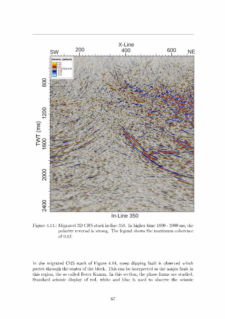
200 400 600
In-Line 350
X-Line
SW NE
Figure 4.14.: Migrated 3D CRS stack in-line 350. In higher time 1600 - 2000 ms, thepolarity reversal is strong. The legend shows the maximum coherenceof 0.02.
In the migrated CRS stack of Figure 4.14, steep dipping fault is observed whichpasses through the center of the block. This can be interpreted as the major fault inthis region, the so called Roter Kamm. In this section, the phase forms are studied.Standard seismic display of red, white and blue is used to observe the seismic
67

CHAPTER 4. 3D SEISMIC IMAGING IN CRYSTALLINE ROCK
section. Red as positive and blue as negative is used as shown in �gure. Thereare blue coloured negative amplitudes between two red coloured amplitudes in thecontinuous event of the fault. From this, it is concluded that, this fault has theproperty of polarity reversal. This can be interpreted that the fault is comprised ofopen fractures. The event is steep dipping and continuous until 2000 ms TWT. Ifthe velocity in this medium is assumed to be 6000 m/s, then the depth of this faultis at about 6 km where it terminates in the subsurface. It is dipping approximatelywith an angle of 70◦.
In Figure 4.13 the indication of the regional fault Roter Kamm is visible as slightindication (in blue coloured amplitude) just below the position of cross-line 200.There are migration smiles visible in imaging of this fault indicating the velocityand aperture issues. This fault is more clearly observed in the migrated coherence.It is important to note that the listric feature of the Roter Kamm is also noticedin the lower part of the fault in this �gure where the fault terminates. In theupper right side of this pro�le, there is coherent di�racted energy visible which isconcentrated at one portion. This is the area of mining activity in past decade. Inthe upper left corner of the pro�le, there are two inclined parallel events dipping inNW direction. These events corresponds to the younger granite and metamorphicrocks as visible in the geological pro�le cross-section.
In the Figure 4.15, which corresponds to cross-line 580, there are two steep dippingevents. These events are dipping in the NNE direction. The steepness of the eventsis approximately 70◦ in dip. These events corresponds to the re�ection of therocks which are intruded in the sub-surface indicated by yellow colour lithologyin the geological map. These are metamorphosed rocks comprising quartzite withclayey schist. The events are well visible as seismic re�ections because of strongimpedance contrast. The event is observed in the subsurface, starting from positionin-line 600 until in-line 100 dipping to the north. The event is continuously visiblein cross-lines starting from cross-line 430 to cross-line 700. The re�ecting eventsterminate in the subsurface at time 2300 ms TWT. In the upper NE area, thecoherent energy is corresponding to the mining area indicated by brown colour inthe geological map of Figure 4.3. At time 2800 ms TWT, there is a small event inthe center which is dipping north. This re�ects a small scale feature in the deepsubsurface. The dip of this event is not as steep as the upper two events (whichstart from the surface).There is a new re�ecting event observed from 3200 ms TWTto 3300 ms TWT. This event is not observed in the migrated stack, but only in themigrated coherence weighted stack or migrated coherence.
Time slices of the seismic volume show features in map view. Events typical for
68

data are explained in time slice 1330 ms TWT Figure 4.16. In this �gure, allthose events are visible which are expected in the subsurface from the previousgeological knowledge. The �gure shows a time slice of migrated coherence. In theNE, the mining zone is visible due to di�racted events and criss-cross pattern. Inthe middle, the conjugate faults are visible which are indicated by arrows. In theSE, the two strips are steep dipping events from clayey schist and quartzite whichare also observed in the cross-line directions. The green coloured arrow shows thedirection of north in the time slice.
Deeper parts of this data show more features then expected and which are notseen in the geological map. The evidence of the Schneeberg body start near thetime 2000 ms TWT. In the time slice of Figure 4.17, the Schneeberg body can beseen in SW close to center. This body is observed continuous throughout someslides. Figure 4.18, Figure 4.19 and Figure 4.20 show that there is continuityof this Schneeberg body with increasing time. In the start of the project, therewas assumption that, the Schneeberg body might be an artifact caused by theacquisition foot print. However the continuity of this feature in some time sliceswith the symmetry raises the argument that this body could be physically existingin nature (subsurface) with the speci�c pattern as observed. This gives the answerof that question with the strong evidence in the time slices of migrated coherencesection. The Schneeberg body could be evolved due to the conjugate faults thatstrike inside the granite body. The crossing pattern of Roter Kamm and conjugatefaults play major role in making the fractured zone. This makes the intersection oftwo fracture systems at the Schneeberg body.
From the observations of the in-lines and cross-lines, it was assumed that theSchneeberg body is just a body acting as a cause for di�racted energy here. But, thetime slices starting from 2000 ms TWT to 2500 ms TWT show that, this body hassome symmetry in it. The Schneeberg body seems to be in a pattern of alphabetX. It seems that two events are crossing here in this sequence perpendicular toeach other. The strong coherent symmetry is striking from SE to NW direction.The other coherent body which is striking from NE to SW direction cross cuts the�rst event.
Comparing to the time slices of migrated coherence with the time slices of coherenceweighted stack (CWS) the later images are cleaner with higher signal to noise ratio.The signal is more pronounced as shown in Figure 4.21. The steep dipping eventsand the pattern of conjugate faults is more clearly visible. Each time slice has itsown eatures, but the structure of either the steep dipping events, the Schneebergbody or the conjugate faults, they are visible throughout some of the time slices.
69

CHAPTER 4. 3D SEISMIC IMAGING IN CRYSTALLINE ROCK
The time slice shown in Figure 4.21 shows most of the features which are indicatedby the geological map. The time slices Figure 4.22 shows the conjugate faults. ThePermian sediments are observed in the north-eastern part of this cube. In Figure4.23, the steep dipping events start to be visible. Down in the cube in time, thesteep event is more strongly noticed as observed in Figure 4.24 and Figure 4.25respectively. The strike of this event is from east to south-west. In the Figure 4.26,at the position where the in-line 400 and cross-line 300 cross each other, there is apattern of scattered energy. This is Schneeberg body. In the migrated coherencetime slice, this structure was strongly imaged, but in CWS the S/N ratio is not asgood. This shows the pattern like two perpendicular fracture systems are crossingeach other. Similar behaviour is noticed near 2100 ms TWT (Figure 4.27) and 2150ms TWT (Figure 4.28). Some other intruded features are noticed at 2700 ms TWTas shown in in Figure 4.29 in north-eastern part near position of in-line 400. Theseevents are deep and no interpretation has been made yet about these events.
Figure 4.30, represents the 3D (migrated coherence) overview of the sub-surfacefeatures of this study area. The block shows the in-line 130, cross-line 600 andtime slice of 2110 ms TWT. The continuity of the events can be observed where thein-lines and cross-lines cross each other. Figure 4.31 showing in-line 148, cross-line650 and time slice 2700 ms gives another view with the CWS. A slight indicationof Roter Kamm is observed between the cross-line number 200-300 for in-line 148.Figure 4.32 with in-line 369, cross-line 650 and time slice 2150 ms indicates theposition of Schneeberg body in 3D which is visible in in-line and also in the timeslice. The inclined clayey schist is also strongly observed in the cross-line. Thecomplexity of the subsurface structure is visualized in these 3D cubes. Figure 4.33gives the sub-surface overview of migrated coherence in transparency to get an ideaof subsurface structure in 3D. Only the strong coherent events are displayed. The3D transparency view allows to observe the nature of these events as structure andtectonics in three dimensional view. The chosen threshold allows us to see only thesignal and unwanted noise is removed to see only structure and get the idea how itlooks like 3D in the subsurface. There are few video animations available with thethesis as electronic supplement in a DVD. The detailed information is available inthe appendix.
70
4.7. Conclusions
Application of a 3D CRS-based work�ow to the Schneeberg 3D hardrock re�ectionseismic data has shown the surprising results. As the S/N ratio of these datais low, the automatic CMP stack showed no signi�cant evidence of any event.The multi-parameter stacking operator provides an alternate approach to theconventional processing of the hardrock data. The data consists of di�ractionsand steep dipping structures. The 3D CRS has provided improved images ofthe sub-surface. The coherence which is an output of 3D CRS work�ow has lowresolution but, it gives more information of the structure and tectonics particularlyfor these data. Although the coherence has low resolution, it is considered as analternate imaging attribute. This is helpful in imaging the hardrock data which isdominated by the di�ractions. Weighting of the coherence (coherence multipliedwith stack) further improved the resultant image which helped in the interpretationof the images. The most prominent feature of this data is the steep dippingre�ection from clayey schist. The conjugate faults are mapped in the migratedcoherence and CWS. Rother Kamm re�ected only faint hints from the seismicsignatures and this behaviour of Roter Kamm was unexpected for the geologists asit was expected to be the most prominent feature of this area. The coherence ofRoter Kamm is less then the conjugate faults. Two fracture systems are imagedwhich are well observed in the time slices of coherence. Some features are still notinterpreted like the re�ections from the higher times more then 2700 ms TWT.Migration needs to be updated with the proper velocity model.
71
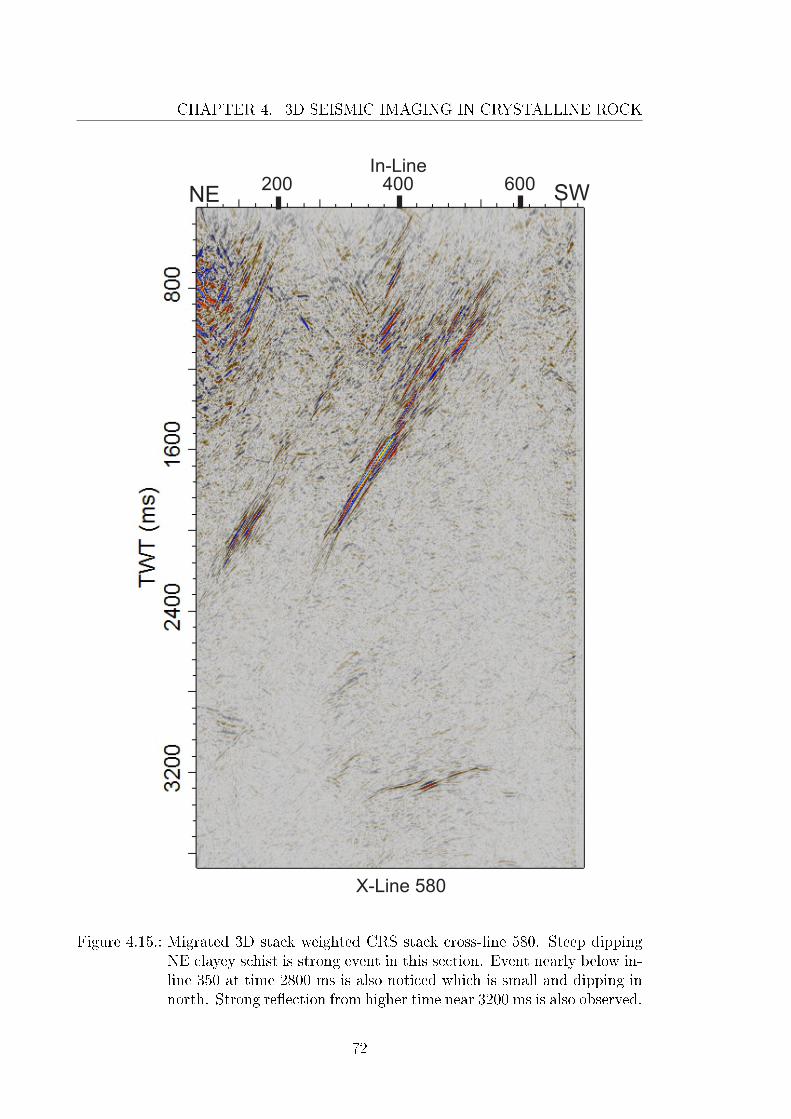
CHAPTER 4. 3D SEISMIC IMAGING IN CRYSTALLINE ROCK
200 400 600In-Line
X-Line 580
NE SW
Figure 4.15.: Migrated 3D stack weighted CRS stack cross-line 580. Steep dippingNE clayey schist is strong event in this section. Event nearly below in-line 350 at time 2800 ms is also noticed which is small and dipping innorth. Strong re�ection from higher time near 3200 ms is also observed.
72
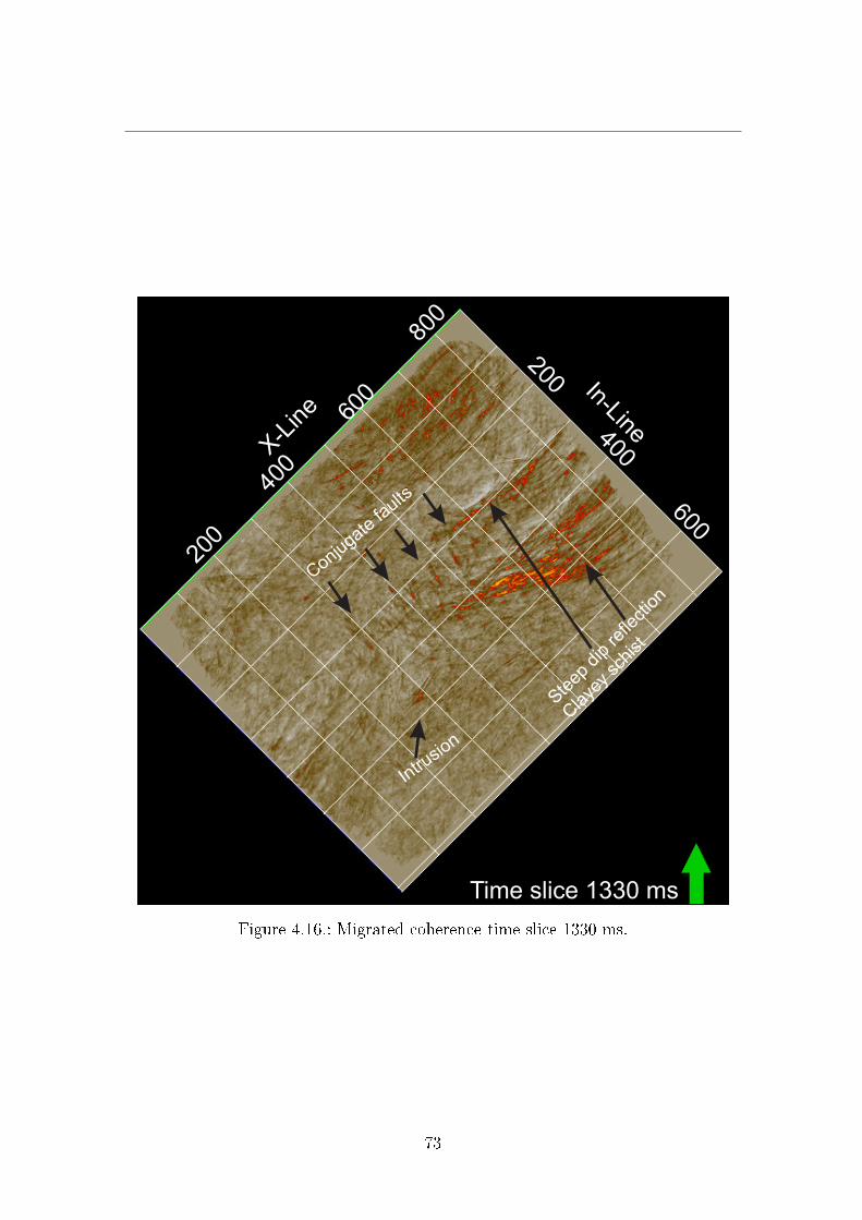
200
400
600
200
400
600
800
Time slice 1330 ms
X-L
ine
In-Line
Steep
dip
refle
ction
Claye
ysc
hist
Conjugate
faults
Intru
sion
Figure 4.16.: Migrated coherence time slice 1330 ms.
73
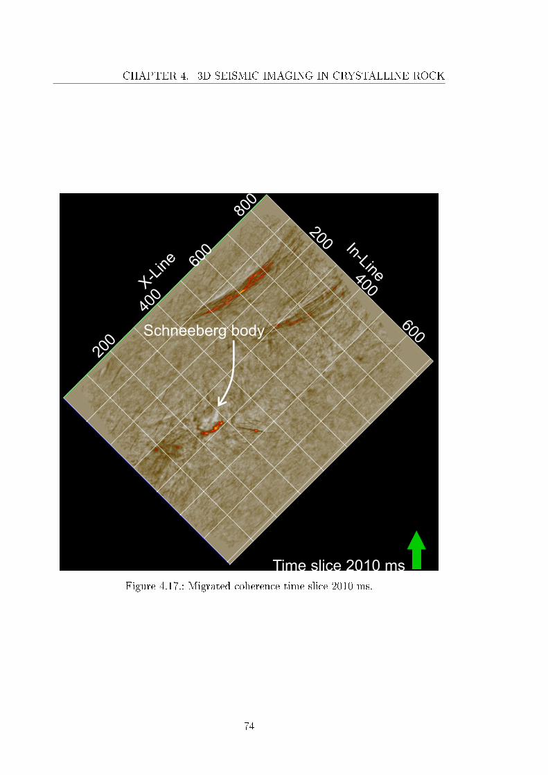
CHAPTER 4. 3D SEISMIC IMAGING IN CRYSTALLINE ROCK
200
400
600
200
400
600
800
Time slice 2010 ms
X-Line
In-Line
Schneeberg body
Figure 4.17.: Migrated coherence time slice 2010 ms.
74
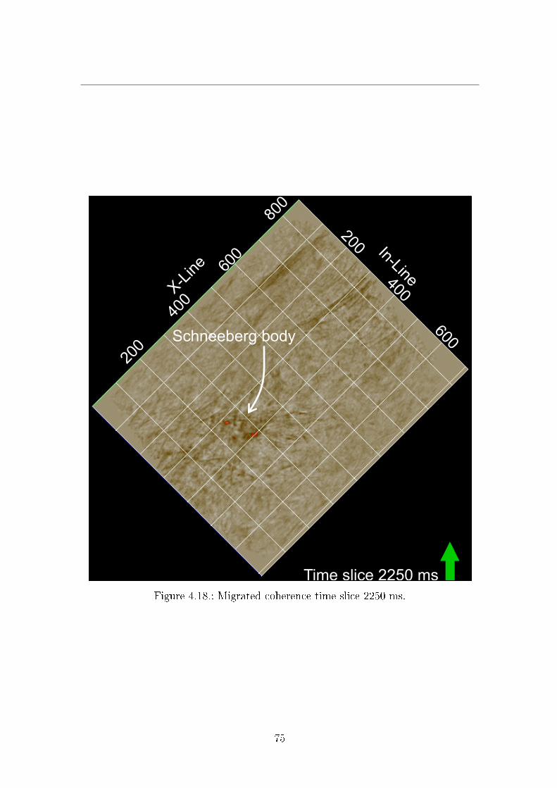
200
400
600
200
400
600
800
Time slice 2250 ms
X-Line
In-Line
Schneeberg body
Figure 4.18.: Migrated coherence time slice 2250 ms.
75

CHAPTER 4. 3D SEISMIC IMAGING IN CRYSTALLINE ROCK
200
400
600
200
400
600
800
Time slice 2340 ms
X-Line
In-Line
Schneeberg body
Figure 4.19.: Migrated coherence time slice 2340 ms.
76
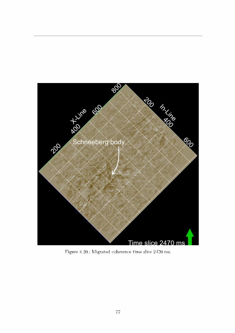
200
400
600
200
400
600
800
Time slice 2470 ms
X-Line
In-Line
Schneeberg body
Figure 4.20.: Migrated coherence time slice 2470 ms.
77
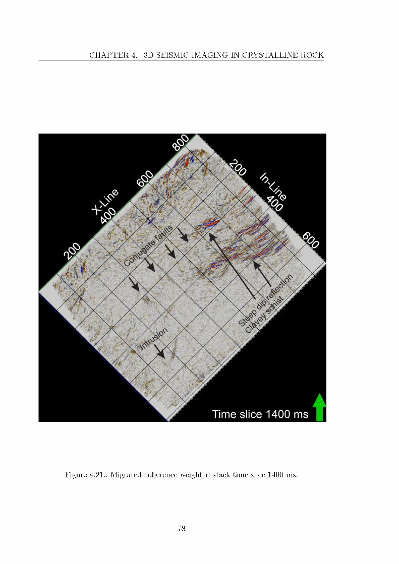
CHAPTER 4. 3D SEISMIC IMAGING IN CRYSTALLINE ROCK
200
200
400
400
600
600
800
Time slice 1400 ms
200
200
400
400
600
600
800
X-Line
In-Line
Steep
dip re
flection
Claye
y sc
hist
Conjugate
faults
Intrusio
n
Figure 4.21.: Migrated coherence weighted stack time slice 1400 ms.
78

200
200
400
400
600
600
800
Time slice 1120 ms
200
200
400
400
600
600
800
Time slice 1120 ms
X-Line
In-Line
Clayey schist
Permian sediments
Figure 4.22.: Migrated coherence weighted stack time slice 1120 ms.
79
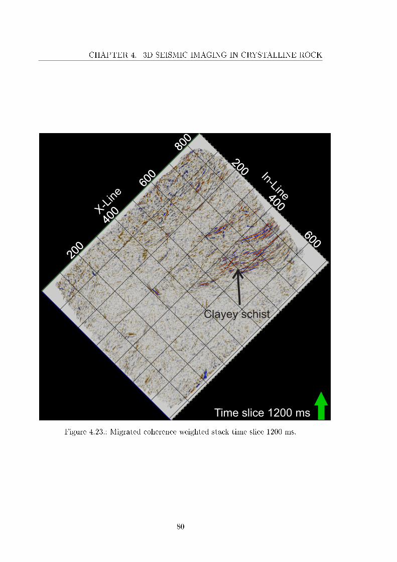
CHAPTER 4. 3D SEISMIC IMAGING IN CRYSTALLINE ROCK
200
200
400
400
600
600
800
Time slice 1200 ms
200
200
400
400
600
600
800
X-Line
In-Line
Clayey schist
Figure 4.23.: Migrated coherence weighted stack time slice 1200 ms.
80
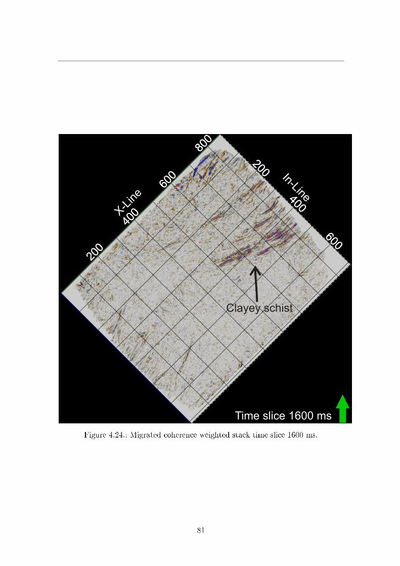
200
200
400
400
600
600
800
Time slice 1600 ms
200
200
400
400
600
600
800
X-Line
In-Line
Clayey schist
Figure 4.24.: Migrated coherence weighted stack time slice 1600 ms.
81

CHAPTER 4. 3D SEISMIC IMAGING IN CRYSTALLINE ROCK
200
200
400
400
600
600
800
Time slice 1800 ms
200
200
400
400
600
600
800
X-Line
In-Line
Schneeberg body
Clayey schist
Figure 4.25.: Migrated coherence weighted stack time slice 1800 ms.
82
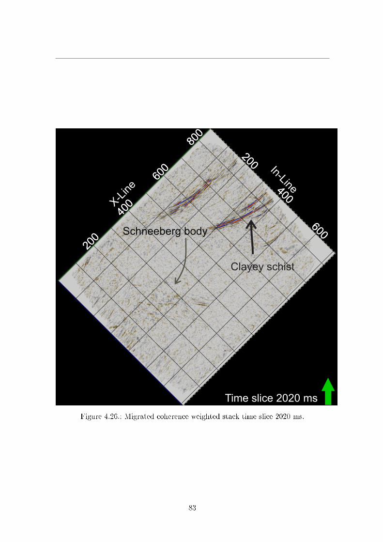
200
200
400
400
600
600
800
Time slice 2020 ms
200
200
400
400
600
600
800
X-Line
In-Line
Schneeberg body
Clayey schist
Figure 4.26.: Migrated coherence weighted stack time slice 2020 ms.
83
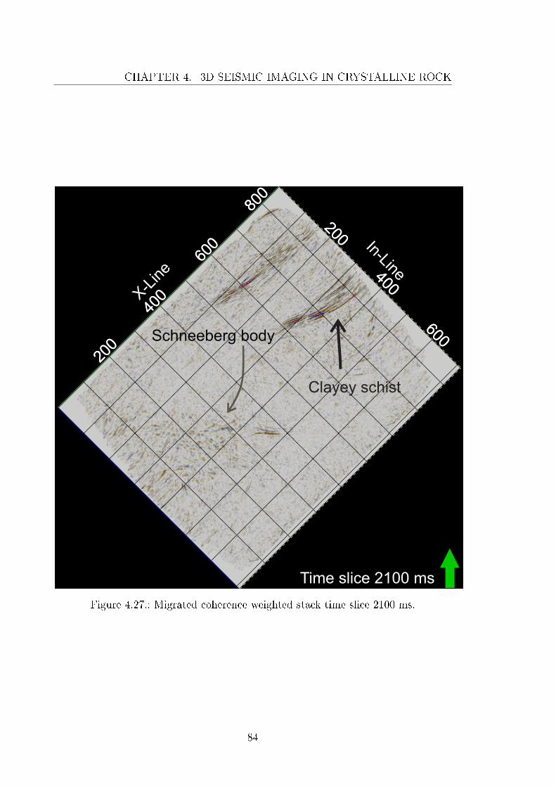
CHAPTER 4. 3D SEISMIC IMAGING IN CRYSTALLINE ROCK
200
200
400
400
600
600
800
Time slice 2100 ms
200
200
400
400
600
600
800
X-Line
In-Line
Schneeberg body
Clayey schist
Figure 4.27.: Migrated coherence weighted stack time slice 2100 ms.
84

200
200
400
400
600
600
800
Time slice 2150 ms
200
200
400
400
600
600
800
X-Line
In-Line
Schneeberg body
Clayey schist
Figure 4.28.: Migrated coherence weighted stack time slice 2150 ms.
85
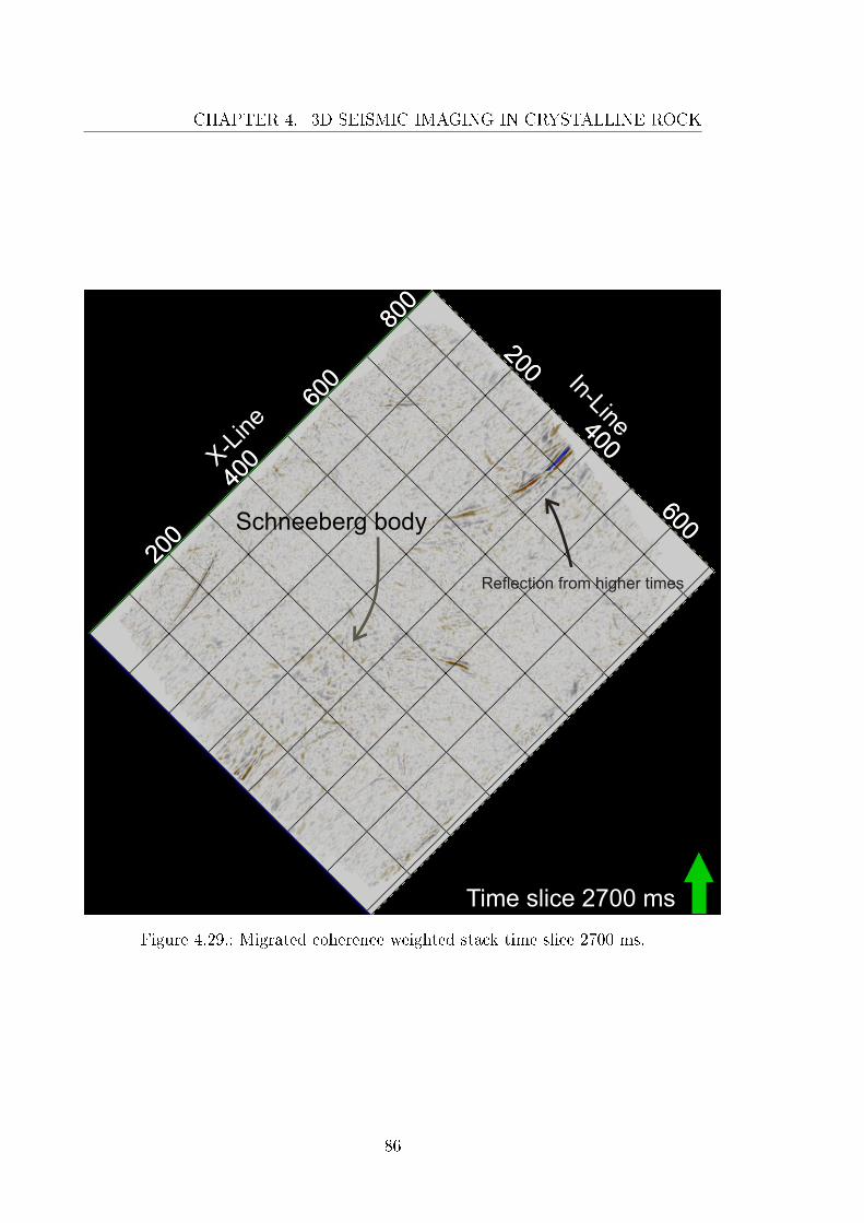
CHAPTER 4. 3D SEISMIC IMAGING IN CRYSTALLINE ROCK
200
200
400
400
600
600
800
Time slice 2700 ms
200
200
400
400
600
600
800
X-Line
In-Line
Schneeberg body
Reflection from higher times
Figure 4.29.: Migrated coherence weighted stack time slice 2700 ms.
86
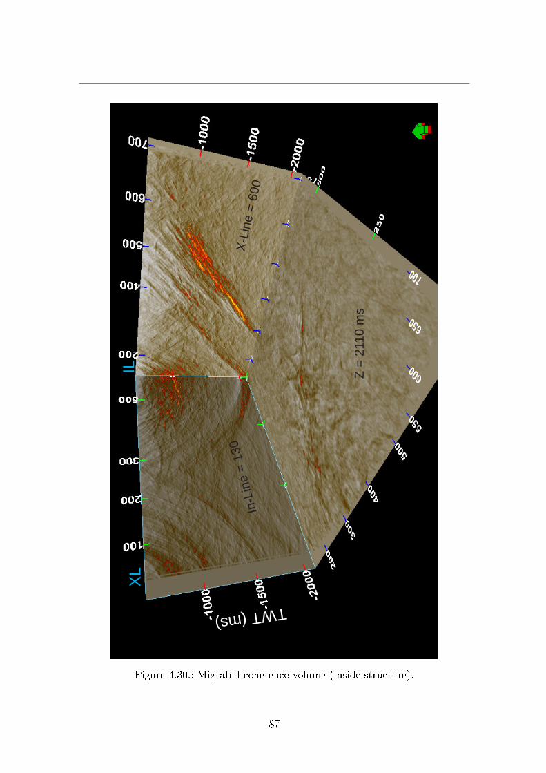
TWT(ms)
Z =
2110 m
s
In-L
ine
=130
X-L
ine
=600
XL
IL
Figure 4.30.: Migrated coherence volume (inside structure).
87
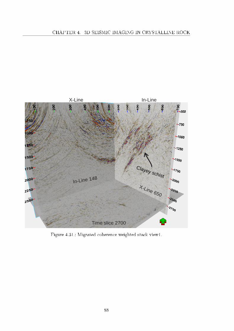
CHAPTER 4. 3D SEISMIC IMAGING IN CRYSTALLINE ROCK
In-LineX-Line
Time slice 2700
In-Line 148
X-Line 650
Clayey schist
Figure 4.31.: Migrated coherence weighted stack view1.
88
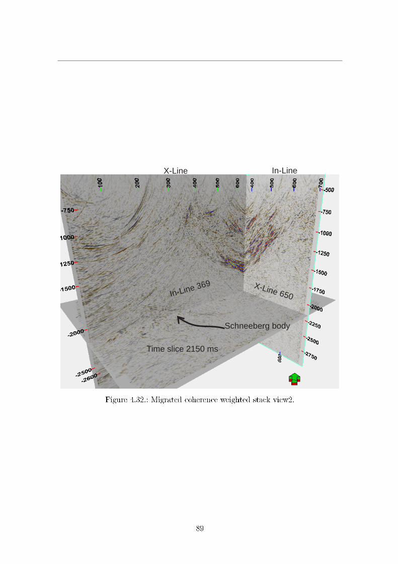
X-Line In-Line
In-Line 369 X-Line 650
Time slice 2150 ms
Schneeberg body
Figure 4.32.: Migrated coherence weighted stack view2.
89

CHAPTER 4. 3D SEISMIC IMAGING IN CRYSTALLINE ROCK
1
2
3
Tim
e(s
ec)
Figure 4.33.: Migrated coherence transparency.
90
5. Summary
Conclusions and discussion
In the present study, there were two important problems to be resolved. One ishow to handle big 3D seismic dataset in feasible time frame. The other is that ifthe data comprising poor S/N ratio and low resolution, how to get a good seismicimage out of it. To solve these problems, two steps were taken. First, to optimizethe parallelization of the 3D CRS code. The original 3D CRS code had problemsrelating to the computation. These problems were relating to memory leaks andthe search strategy. Also not all of the available resources were being utilized whilecomputing the search steps.
In the 3D CRS work�ow, almost 90-94% of the computational cost is utilized bycoherence analysis. In modern machines, there are virtual cores and the threadsavailable on CPUs. To improve the optimization (MPI based code), the code wasoptimized that the output is saving the time and cost both. In ideal conditions,the e�ciency is up-to 10 times faster. Under special conditions, the e�ciency iseven more better than that. All e�ort to optimize (hybrid MPI with OpenMP) thecode is to generate the threads that can be utilized in the processing if available onmachines and cumulative performance gets better.
Upto now, the studies using the hybrid approach reveal that, the performance ofthis code is improved. Some tests on 2D, small 3D data proved that it is coste�cient and can save days, weeks, and even months when the data is huge. Thiscode was tested on the Schneeberg 3D seismic dataset. The data was 500 GB involume which is quite huge by academic standards. The hybrid code is able tohandle it e�ciently. The output of old code is similar to the new hybrid code. Thecode works more e�ciently in the shared memory architecture than parallel memorybecause of the demand of the code. The data tunneling and communication isbetter in the new code. However, there are still some issues like memory leaks andsome search strategies are not so well optimized. The code still needs to be writtenfrom scratch in a professional style in order to achieve better results in terms of
91

CHAPTER 5. SUMMARY
e�ciency. For the Schneeberg 3D seismic dataset, the code worked fairly well.Thus the high performance computing (HPC) helped a lot in working with thehuge datasets. Although the e�ciency is not reached to the industrial level wherespecialized hardware for high performance computing like GPUs and FPGA is used.For the academic level, the performance of accelerated code is quite satisfactory.This is a leap in leading towards the improvement in the e�ciency of code.
Application of a 3D CRS-based work�ow to the Schneeberg 3D hardrock re�ectionseismic data is purely a data-driven approach. The S/N ratio of these data isvery low and the initial automatic CMP stack indicated that multi-parameterprocessing methods, which use more traces in the stack might improve the imagequality. Although the comparison of conventional CMP stacking with automaticCMP stacking is unfair, but the studies show that the conventional CMP stackinghas not produced the reasonable results from these hardrock dataset (Lüschen et al.2015. The data are dominated by di�ractions generated at various steep dippingfracture zones. Steep structures and a huge number of di�raction tails interfereor lead to a complicated pattern of con�icting dips. The CRS stack showed aconsiderably improved S/N ratio and provided a reasonable basis for geologicalinterpretation. However, plots of the coherence actually delivered good imagesfor interpretation for this particular type of hardrock data. Despite the reducedresolution compared to the stack, the coherence is considered as a suitable imagingattribute, since it is an objective measure of the local similarity in the wave�eldand directly re�ects the physical relevance of the corresponding seismic event. Forthe considered data the coherence is a data-driven imaging attribute particularlyhelpful for the interpretation of hardrock data. Weighting, i. e., multiplying thestacks with the coherence further improved the S/N ratio of the resulting sectionsand supported the interpretation of the images. Similar conclusions apply to thedisplay of the coherence-weighted time slices, which provided the best images.
The re�ections from top and bottom of the clayey schists represent the mostprominent features in the data. A sequence of conjugate faults is also nicelymapped. Their lateral extent at depth seems to be small which does not coincidewith the surface expression of these faults. There are some surprised resultsrevealed from the study of these hardrock dataset. Prior to this experimentthe Roter Kamm was expected to be the most prominent structure in the data.However, it is noted that there are only faint hints of this fault in the data andthe respective coherence is much smaller than the coherence of the sequence ofconjugate faults. Another prominent feature of the data was detected in the SW ofthe survey area. This feature represents a region with a very high number of alignedevents below 1.5 s TWT named as Schneeberg body. This area of high coherenceis located in a region where several fracture systems intersect and may have ahigh fracture density. Whether these fractures are open or mineralized cannot be
92

decided from the current state of processing. Open fractures would make this area afavorable region for a geothermal heat exchanger. It is known, however, that manyfracture systems in the North of the measurement surface are mineralized, whichinitiated the mining activities in this area. Di�erent features are still un-interpretedspecially in higher traveltime and several are still unexplored due to the data quality.
93

6. Outlook
Many options are open for optimizing the 3D CRS code, like sorting problem of thememory leaks and the data I/O etc. One way to get the high performance computingwith 3D CRS code is to rewrite it for modern hardware. However analyzing theparts of the code (which needs to be optimized) also needs considerable time. Thealternating approach is to convert the code into FPGA (�eld programmable gatearray) based code which is also possible with either the hardware design languageor using the Max-compiler on Maxeler machine.
Imaging Schneeberg data from crystalline environment opened new horizons tothink about the problems which are faced during the seismic data processing fromcomplex environment and it rails the research in di�erent directions to improvethe S/N ratio of seismic data. Pre-stack time and depth migration of hardrockdata will rely on the respective velocity model input. Because of the poor dataquality, the estimation of CRS attributes is not necessarily stable and all processesrelying on these attributes may be compromised. This includes the computationof migration velocities. All options to improve the signal quality of the pre-stackseismic data will help to better image the subsurface of hardrock systems. Keyelement in the successful processing of hardrock data is the enhancement of thepre-stack data quality. Partial CRS stacks (e.g., Baykulov and Gajewski 2009)might be an option to improve the data quality in the pre-stack domain. Seismicdata from a hardrock subsurface are largely dominated by di�ractions, which arenot optimally �tted by the CRS operator. Processing the data with the i-CRSoperator (e.g., Schwarz et al. 2014) might improve the determination of wave �eldattributes, since it better �ts di�ractions. High quality attributes will result in morereliable time migration velocities, capable of improving NIP wave tomography andbetter pre-stack data enhancement opportunities. Another option of pre-stack dataimprovement is given by the partial time migration introduced by (Dell et al. 2012).This tool also has a pre-stack data enhancement facility and requires reasonable timemigration velocities to be applied e�ectively. 3D NIP wave tomography (Klüver,2007) can be used to estimate the velocity model using the attributes by pickingreliable events. Anisotropy is one of the main targets which can help in betterimaging such type of dataset. Con�icting dips are main issue in CRS processingand can lead to wrong estimation or lead to the loss of events in the stacked section.
95

CHAPTER 6. OUTLOOK
Handling con�icting dips in 3D CRS processing can lead to improvement in theimaging of criss-cross patterns in the stacks. The method suggested by (Waldaand Gajewski, 2015) can be implemented for 3D case to resolve this issue. As thedata is dominated by di�ractions, a specialized processing and tomography recentlydiscussed by (Bauer, 2014) and (Schwarz, 2015) may lead to a new methodology forvelocity model building entirely based on zero-o�set data.
96
A. Electronic Supplements in
DVD
∗ In the DVD, there are animated videos with slide shows of 3D volumes fromdi�erent directions and di�erent angles. These volumes are imaged withthe transparency. This means that there is certain threshold for the signalto visualize. Most of the noise is attenuated which is below the threshold.Therefore most of the signal is visible and the unwanted noise disappears.Di�erent colour scales are used to visualize the volumes. The videos are ofmigrated coherence weighted stack, migrated coherence (animated slides) andmigrated stack.
∗ Electronic pdf version of thesis is also available.
∗ The DVD supplement is not available online and can be accessed on requestfrom the department library or by writing an email [email protected].
97

Used softwares and hardwares
During the research work, di�ernet types of operating systems have been used, whichare Linux (Debian and CentOS) free version licenses and (Windows XP/7/8.1).
The hybrid approach for High Performance computing (HPC) developed in thisthesis is based on 3D ZO CRS stack code as implemented by Alex Müller (2007),concurrent programming using C++ and integrated approach to use (OpenMP withMPI) for using the threads. This has been successfully implemented and done withthe help of DKRZ (Specially Dr. Hendryk Bockelman).
Migration of the 3D seismic volumes has been done by using the ProMAX &SeisSpace software from Hilliburton.
For visualization of the 3D cubes and inlines, crosslines, slices, Opendtect, Petrel(Seismic to simulation) from Schlumberger, Seismic Un*x (Colorado School of Mine)were used.
For some visualization, drawing, editing and generating images, Corel Draw(Graphic suit X6) and Inkscape has been used.
SeisSee (free) has been used for header investigation.
For animation and 3D visualization, Avizo Earth (in collaboration of DKRZ) hasbeen used.
The Wave Inversion Technology (WIT) consortium provided further software for theCRS processing:
1. 3D ZO CRS stack (by Alex Müller)
2. Automatic picking of input data for tomographic inversion (by Tilman Klüver)
3. 3D NIP-wave tomography (by Tilman Klüver)
4. 3D Migration velocity analysis for di�ractions (by Sergius Dell)
99

APPENDIX A. ELECTRONIC SUPPLEMENTS IN DVD
5. 3D Di�raction mapping
6. C/C++ for programming
Four types of hardware machines have been used:
1. Desktop machine core i7 based.
2. Tornado (little endian) 2000cores based.
3. Thunder (little endian) cluster 32cores (64 threads) based.
4. Blizzard (bigger endian) cluster 8000 cores based.
5. Laptop core i5 based.
The thesis is written on laptop and desktop based OS in LATEX.
100
Aknowledgements
� I have no words to express my humble thanks and love to Professor Dr. DirkGajewski for accepting me as PhD student, giving me chance to work under hissupervision and gave me lot of freedom to express my skills. It is his highnessthat he trusted me while accepting even without knowing me. His door wasalways open for every problem and help either in research or moral support isneeded. He gave me the opportunity to express my research across the globein conferences and meetings.
� I am also grateful to Dr. Claudia Vanelle for the co-supervision of my thesisand also for allowing me to further develop my skills. Special thanks for theproof reading of this thesis.
� I would also like to say thank you to Dr. Hendryk Bockelman from DKRZ forsharing precious ideas and sparing time to resolve issues relating to softwareand coding.
� I am thankful to Benjamin Schwarz for sharing o�ce, we did lot of beni�cialdiscussions and we shared every feeling and problem and resolved together. Ialways enjoyed his company.
� I would also like to say thank you to Dr. Sergius Dell from CGG, London, forsharing o�ce, nice discussions, wonderful ideas of seismic imaging and alwaysbeing helpful in every problem.
� I also like to say thank you to Dr. Ekkehart Tessmer for being with me inevery time of di�culty relating to computer, cluster and coding and all otherproblems which I share to him.
� I am as well grateful to Dr. Mikhail Baykulov (Addax Petroleum) for sharingwonderful ideas relating to research.
� I am thankful to Dr. Christian Hübscher for giving nice advices and discussionsrelating to my work.
101

APPENDIX A. ELECTRONIC SUPPLEMENTS IN DVD
� I would like to say thanks to Dr. Ali Dehghani for always being helpful.
� Helping e�ort of Dela Spickermann and Michael Böttinger from DKRZ is alsoappreciated specially for visualization and animations.
� Thanks to Prof. Dr. Boris Kashtan from Russian Academy of Sciences, SaintPetersburg, Russia for nice helpful discussions.
� Discussions with project parteners from LIAG, Hannover and TU Freiberg isalso appreciated.
� Thanks to Prof. Dr. Zul�qar Ahmad and Prof. Dr. Shahid Nadeem Qureshifor always encouraging me for research work.
� My special thanks also goes to Christel Mynarik and specially Paola Dal Corsowho always helped me with administration issues.
� I would like to thanks Hendrik Niehaus, Leonie Pick, Jan Walda, Malik FaisalPeracha, Ivan Abakumov, Phillip Witte, Martin Vögele, Muayyad YounisMahmoud Al Hseinat, Mahmood Sultan, Syed Faraz Ahmed, Syed AwaisHaider and Shehzada Yasir Ummar for always being with me for support andhelp during my PhD.
� I gratefully acknowledge the Wave Inversion Technology (WIT) consortium forfunding of my position and the conference attends. The Code provided by theconsortium represents the basis for the work presented in this thesis.
� I like to thank BMWi for data and �nancial support. Funding by the FederalMinistry for Economic A�airs and Energy of Germany (0325363A) is gratefullyacknowledged
� Obviously, I like to say in�nite thanks to my family starting from specially myparents, father Ashfaq Ahmed Qazi, mother Nighat Yasmin, wife Hira Khawar,brother Khurram Ashfaq Qazi for always being with me in any situation andalways supporting me �nancially, physically, morally and spritually in myprogress. They always standby on my decisions and never let me down in anydi�cult situation. Thanks to my beloved brother Manazar Ahsan Hashmi,sister Asma Manazar, and nephew Abdul Moiz Hashmi and Abdul AzeemHashmi for giving me in�nite love and moral support. Indeed, I am incompletewithout any of them in my life.
� Always thanks to Almighty ALLAH for blessings on me.
102

Bibliography
M. Al-Chalabi. Series approximation in velocity and traveltime calculation.Geophysical Prospecting, 21(4):783�795, 1973.
A. Bauer. From zero-o�set to common-o�set with di�ractions. Master's thesis,University of Hamburg, 2014.
M. Baykulov. Seismic imaging in complex media with Common Re�ection SurfaceStack. PhD thesis, University of Hamburg, 2009.
M. Baykulov and D. Gajewski. Prestack seismic data enhancement with partialcommon-re�ection-surface (CRS) stack. Geophysics, 74(3):V49�V58, 2009.
M. Baykulov, S. Dümmong, and D. Gajewski. From time to depth with CRSattributes. Geophysics, 76(4):S151�S155, 2011.
H. J. Berger, M. Felix, S. Görne, E. Koch, O. Krentz, A. Förster, H. J. Förster,H. Konietzky, Ch. Lunow, K. Walter, H. Schütz, K. Stanek, and St. Wagner.Tiefengeothermie Sachsen. Number 9 in Schriftenreihe. Landesamt für Umwelt,Landwirtschaft und Geologie, 2011.
S. Bergler, P. Hubral, P. Marchetti, A. Cristini, and G. Cardone. 3D common-re�ection-surface stack and kinematic wave�eld attributes. The Leading Edge, 21(10):1010�1015, 2002.
W. Bruce, N. Flesjå, O. E. Kristiansen, F. Vignati, A, and A. Aronsen, H. Shallowwater 3D multiple attenuation:A case study in methods. WorldOil, 2009.
B. Chapman, G. Jost, and R. Van Der Pas. Using OpenMP : portable shared memoryparallel programming. The MIT Press, Cambridge, Massachusetts, London,England, 2008.
J. F. Claerbout. Imaging the Earth's Interior. Blackwell, 1985.
J. F. Claerbout and S. M. Doherty. Downward Continuation of Moveout CorrectedSeismograms. Geophysics, 37(5):741�768, 1972.
S. Dell and D. Gajewski. Common-re�ection-surface-based work�ow for di�ractionimaging. Geophysics, 76(5):S187�S195, 2011.
103
Bibliography
S. Dell, D. Gajewski, and C. Vanelle. Prestack time migration by common-migrated-re�ector-element stacking. Geophysics, 77(3):S73�S82, 2012.
S. Dümmong and D. Gajewski. A multiple suppression method via CRS attributes.2008 SEG Expanded Abstracts, pages 2531�2535, 2008.
E. Duveneck. Velocity model estimation with data-derived wavefront attributes.Geophysics, 69(1):265�274, 2004.
D. W. Eaton, B. Milkereit, and M. H. Salisbury. Hardrock seismic exploration.Number 10. SEG Books, 2003.
R. Emmermann and J. Wohlenberg. German Continental Deep Drilling Program(KTB). Springer, 1988.
S. Fomel. Velocity analysis using AB semblance. Geophysical Prospecting, 57:311�321, 2009.
J. Gazdag. Wave equation migration with phase-shift method. Geophysics, 43:1342�1351, 1978.
B. Gelchinsky, E. Landa, and V. Shtivelman. Algotithm of phase and groupcorrelation. Geophysics, 50:596�608, 1985.
N. A. Gnatus, M. D. Khutorskoy, and V. K. Khmelevskoi. Petrothermal Energy andGeophysics., volume 66. Moscow University Geology Bulliten, Allerton Press,Inc.,ISSN 0145-8752, 2011.
H. P. Harjes, K. Barm, H. J. Dürbaum, H. Gebrande, G. Hirschmann, M. Janik,M. Klöckner, E. Lüschen, W. Rabbel, M. Simon, J. Thomas, J. Tormann, andF. Wenzel. Origin and nature of crustal re�ections: Results from integratedseismic measurements at the KTB superdeep drilling site. Journal of GeophysicalResearch, 102(B8):18,256�18,288, 1997.
T. Hertweck, J. Schleicher, and J. Mann. Data stacking beyond CMP. The LeadingEdge, 26:818�827, 2007.
P. Hubral. Computing true amplitude re�ections in a laterally inhomogeneous earth.Geophysics, 48(8):1051�1062, 1983.
P. Hubral and T. Krey. Interval velocities from seismic re�ection traveltimemeasurements. Soc. Expl. Geophys., 1980.
R. Jäger, J. Mann, G. Höcht, and P Hubral. Common-re�ection-surface stack:Image and attributes. Geophysics, 66:97�109, 2001.
T. Klüver. Velocity model building using analytic and model-based di�ractiontraveltime functions. PhD thesis, University of Karlsruhe, 2007.
104
U. Kroner, T. Hahn, R. L. Romer, and U. Linnemann. The variscan orogeny inthe Saxo-Thuringian zone - Hetrogeneous overprint of Cadomian/paleozoic Peri-Gondwana crust., volume 423. Geological Society of America, Spec. Pap.� 2007.
S. A. Levin. Principle of reverse time migration. Geophysics, 49(5):581�583, 1984.
U. Linnemann and R. L. Romer. Pre-Mesozoic Geology of Saxo-Thuringia (Fromthe Cadomian Active Margin to the Variscan Orogen). Schweizerbart SciencePublishers., 2010.
S. Luo and D. Hale. Velocity analysis using weighted semblance. Geophysics, 77(2):U15, 2012.
E. Lüschen and R. Schulz. 3-D Seismic Surveys Explore German PetrothermalReserves. EOS Transactions, American Geophysical Union, 95(26):237�244, July-2014.
E. Lüschen, S. Görne, H. von. Hartmann, R. Thomas, and R. Schulz. 3Dseismic survey for geothermal exploration in crystalline rocks in saxony, germany.Geophysical Prospecting (Special Issue Hardrock), 2015.
A. Malehmir, R. Durrheim, G. Belle�eur, M. Urosevic, C. Juhlin, D. J. White,B. Milkereit, and G. Campbell. Seismic methods in mineral exploration and mineplanning: A general overview of past and present case histories and a look intothe future. Geophysics, 77(5):WC173�WC190, 2012.
J. Mann, R. Jäger, T. Müller, and P. Hubral. Common-re�ection-surface-stack - areal data example. J. Appl. Geoph, 42(3,4):283�300, 1999.
W. H Mayne. Common re�ection point horizontal data stacking techniques.Geophysics, 27:927�938, 1962.
B. Milkereit, E. K. Berrer, A. R. King, A. H. Watts, B. Roberts, E. Adam, D. W.Eaton, J. Wu, and M. H. Salisbury. Development of 3-D seismic explorationtechnology for deep nickel-copper deposits-A case history from the Sudbury basin,Canada. Geophysics, 65(6):1890�1899, 2000.
N-A. Müller. Determination of interval velocities by inversion of kinematic 3Dwave�eld attributes. PhD thesis, TH Karlsruhe, 2007.
Nils-Alexander Müller. The 3D Common-Re�ection-Surface stack � Theory andapplication. Master's thesis, University of Karlsruhe, 2003.
N. S. Neidell and M. T. Taner. Semblence and other coherency measures formultichannel data. Geophysics, 36:482�497, 1971.
J. A. Nelder and R Mead. A simplex method for function minimization. ComputerJournal, 7:308�313, 1965.
105

Bibliography
H. Paschen, D. Oertel, and R. Grünwald. Possibilities of geothermal electricitygeneration in Germany (in German with English abstract). TAB Rep. 084, O�.of Technol. Assess, German Bundestag, Berlin, 2003.
Schlumberger. Oil�eld glossary, 2015.
W. A. Schneider. Integral formulation for the migration in two and three dimensions.Geophysics, 43:49�76, 1978.
B. Schwarz. Moveout and Geometry. PhD thesis, University of Hamburg, 2015.
B. Schwarz, C. Vanelle, D. Gajewski, and B. Kashtan. Curvatures andinhomogeneities: An improved common-re�ection-surface approach. Geophysics,79(5):S231�S240, 2014.
R. H. Stolt. Migration by fourier transform. Geophysics, 43:23�48, 1978.
R. H. Stolt. Seismic data mapping and reconstruction. Geophysics, 67:890�908,2002.
R. H. Stolt and A. K. Benson. Seismic migration theory and practice. GeophysicalPress, London, page 382pp, 1986.
M. T. Taner and F. Koehler. Velocity-spectra digital computer derivation andapplications of velocity functions. Geophysics, 34:859�881, 1969.
J. Walda and D. Gajewski. Handling the Con�icting Dip Problem in the CRS/i-CRSMethods. In 77th Annual International Meeting, EAGE, page WS06. ExpandedAbstracts, 2015.
A. Williams. C++ Concurrency in Action (PRACTICAL MULTITHREADING).Manning Publications Co. PO Box 261 Shelter Island, NY 11964, USA, 2012.
O. Yilmaz. Seismic Data Processing, Vol. I and II. SEG, Tulsa, 2001.
106