3 Continuous Numerical outcomes - macmillanihe.com resources (by Author)/S... · The reason is that...

Contexts

What is this chapter about?

In this chapter we consider the probabilities associated with continuous random variables; that

is, numerical outcomes that can take any value within a range – for instance, the height of a

20-year-old male, the duration of a call to a call centre, or the depth of the sea at a randomly

chosen point.

Why is it useful?

As we said in the previous chapter, the ability to predict the likelihood of various values is

invaluable for planning and decision making. This chapter widens the repertoire of ‘patterns’ of

probabilities or probability distributions. In particular, it includes the most commonly occurring

distribution: the normal distribution, which is essential for inferential statistics.

Where does it fi t in?

Much of the subject of Probability is concerned with the probabilities associated with random

variables; that is, measurements that take an uncertain numerical value. There are two types

of random variable: discrete and continuous. The last chapter (P2) was concerned with discrete

random variables and this chapter considers continuous random variables.

What do I need to know?

You must be at ease with the last two chapters (P1 and P2) and, of course, with the material in

Essential Maths.

Objectives

After your work on this chapter you should be:

• able to use a probability density function (pdf) to represent the probabilities associated with

a continuous random variable;

• able to calculate the probabilities associated with the uniform distributions;

• familiar with the normal distribution and the standard normal distribution and able to

calculate their probabilities using tables or a computer.

Our actions are only throws of the dice in the sightless night of chance

Franz Grillparzer, Die Ahnfrau

P

309

3 Continuous Numerical outcomes

After considering discrete random variables in Chapter P2 we now move on to continuous random variables – that is, random variables that can take any value within a range.

We start this chapter by introducing the probability density function (pdf) of a continuous random variable and showing how probabilities can be calculated from it. The normal distribution is particu-larly important as it is perhaps the most widely used distribution and it plays a key role in Statistics.

1 Probability density functions (pdfs)A continuous random variable is a random variable that can take any value within a range, as in the following examples.

• The annual rate of infl ation for the UK.• The time it takes a runner to complete a marathon.• The time it takes a particular Formula One racing driver to complete a lap at the Monaco Grand

Prix.• Human body temperature when in good health.• The time between phone calls received at a switchboard.• The weight of a new-born baby.• The amount of your electricity bill in the winter quarter.

Notice that continuous random variables are usually measurements as opposed to ‘counts’. Contrast these with discrete random variables that can only take a selection of values within their range, for instance, the number of cars that pass a motorway check-point in a minute, or the number of students who pass an exam out of a class of 30.

The probability distribution of a continuous random variable

We already know that the probability distribution of a discrete random variable is a list of all its possible values and their probabilities. For example, a typical probability distribution for a discrete random variable, X, might be

x P(x)

0 0.01

1 0.5

2 0.4

3 0.07

4 0.02

Before you read on, can you see why we can’t represent the probabilities of a continuous random variable in the same way?

The reason is that a continuous random variable can take any value within its range and so a list of all the possible values would be infi nitely long. For instance, the time it takes a runner to complete a marathon can be recorded to any number of decimal places and so, in theory, an infi nite number of different times are possible. In practice of course, the time will only be recorded to the nearest tenth or hundredth of a second, and so there will be a very large number rather than an infi nite number of possible times.

So, we do not write down the probability distribution of a continuous random variable in the manner shown above because the number of probabilities required would be infi nite or, at best, prohibitively large. Also, as the total of the probabilities in a probability distribution has to be 1, most of these probabilities would be extremely small.

To avoid this problem, the probability structure associated with a continuous random variable is represented using a probability density function (pdf) (sometimes just called the probability distribution again). The graph in Figure 3.1 shows the pdf of a random variable, X. As you can see, it is just a curve that lies on or above the x axis of a graph.

310 PROBABILITY 3

50x

f (x )

10 15 20 25

Figure 3.1 A probability density function.

The pdf is chosen so that the area underneath the curve between any two values on the x axis is the probability that X falls between these two values. For instance, area A in the graph in Figure 3.2 shows the probability that X lies between 10 and 15, P(10 < X < 15) and area B shows the probability that X is less than 5; that is, P(X < 5).

B

A

50 10 15 20 25

P(X < 5)

x

f(x)

P(10 < X < 15)

Figure 3.2

It follows that the total area under a pdf curve must be 1 because the probability that X takes a value that lies somewhere on the x axis is 1.

The pdf curve is usually given by a formula in x which we will refer to as f(x). For instance, the pdf shown in Figures 3.1 and 3.2 is f(x) = 0.1e–0.1x, where e is just the number 2.71828… as usual.

As another example, consider the pdf in Figure 3.3. As before, the area under the whole curve is 1 but this time X can take both positive and negative values. Area C is the probability that X lies between –1 and 1.5.

C

–4 –3 –2 –1 10 2 4x

(x)f

P(–1 < X < 1.5)

3

Figure 3.3

CONTINUOUS NUMERICAL OUTCOMES 311

P

The pdf of a random variable X is a curve, given by the formula f(x), with the following properties:

(i) it lies on or above the x axis,(ii) the area under the whole curve is 1, and(iii) the area under the curve between any two values a and b is P(a < X < b).

check this Which of the sketches in Figure 3.4 could be pdfs?

f (x )

x

a.

f (x )d.

f (x )

x

x

b.

1

00

0

100

f (x )

x

c.

1

0

Figure 3.4

Solutions:a. and d. could be pdfs, provided that the scale on the horizontal axis is such that the area underneath the curve is 1. The area under the curve in b. is 100 so this cannot be a pdf. The curve in c. goes below the x axis and so could not be a pdf.

As a continuous random variable can take an infi nite number of possible values, the proba-bility that it takes any individual one is 0. This means that for continuous random variables it doesn’t matter whether we talk about, for instance, P(X < 5) or P(X 5), or about P(–1 < X < 1.5) or P(–1 X 5) because the end points of any interval contribute a zero probability.

Using pdfs for discrete random variables

When a discrete random variable has a huge number of possible values it is impractical to work with the (discrete) probability distribution.

For instance, suppose a large motor manufacturer sells between 10,000 and 12,000 cars inclusive a month. The discrete probability distribution of X, the number of cars sold in a month, contains 2001 probabilities, P(X = 10,000), P(X = 10,001), P(X = 10,002) and so on up to P(X = 12,000), and the probabilities which are usually of interest like P(X > 10,500) or P(X < 11,700) are generally the sum of many of these. This is cumbersome and we are not likely to be able to estimate all 2001 probabilities accurately. It is much easier to represent the probabilities approximately using a pdf (maybe like the one in Figure 3.5) and treat car sales as a continuous random variable. Any errors due to the fact that X is really discrete are usually small.

10,000

f (x )

11,000 12,000x

Figure 3.5

312 PROBABILITY 3

Pdfs and histograms

Suppose X is the duration of the working life of a type of electronic chip. The manufacturer takes a sample of 20 such chips and tests their lifetimes. A histogram of the lifetimes of these 20 chips is shown in Figure 3.6.

0 20 40 60 80 100 120 140 160

Figure 3.6 Histogram of the lifetimes of a sample of 20 chips.

The distribution is clearly skewed to the right. A larger sample, of 100 chips, gives the histogram in Figure 3.7.

0 20 40 60 80 100 120 140 160


This has a similar general shape to the histogram in Figure 3.6 but shows a little more detail because the class width can be narrower as there are more data. A sample of 2000 chips gives the histogram in Figure 3.8, which is even fi ner.

0 20 40 60 80 100 120 140 160



P

We could continue by taking larger and larger samples. As the size of the sample increased the class width could be reduced further and the corresponding histograms would gradually approach the shape of the pdf of the lifetime of a chip, which is shown in Figure 3.9.

f (x )

x160140120100806040200

Figure 3.9 Pdf of the lifetime of a chip.

So the pdf can be regarded as the histogram of an infi nite number of repetitions of the random variable. (We had a similar result for discrete random variables – that the relative frequencies of a large number of values of a discrete random variable approach the probabilities (see p. 295).)

Drawing pdfs

To get a feel for pdfs try sketching a rough pdf for the following random variables. Remember that you are really just drawing a histogram of lots of repetitions of the random variable.

check this Draw a rough graph of a plausible pdf for the following random variables.

a. The age of an undergraduate student selected at random from your university.b. The number of minutes to the next bus, when you have just missed one.c. The winning ticket in a lottery in which 10,000 tickets are numbered consecutively from 1 to

10,000.d. The height of an adult man.e. The height of an adult woman.f. The height of an adult.

Solutions:No exact answers are possible here – it depends what is assumed about the random variable of interest. We suggest the following sketches.

f (x )

a.

x17

f (x )

c.

x1

f (x )

e.

x

f (x )

b.

x0

f (x )

d.

x168

f (x )

f.

x154154

70 25 10000

168

314 PROBABILITY 3

check thiscontinued

a. We have assumed that a student cannot be younger than 17, that the ages between about 18 and 22 are most common and that the higher the age above this, the less common it is.

b. We have assumed that until a due time of 20 minutes the bus becomes more likely to arrive, and that one is certain to arrive within 25 minutes.

c. This is a discrete random variable but there are 10,000 possibilities so we can approximate the probability distribution using a pdf. Each ticket number is equally likely so the pdf has equal height throughout the range.

d. We have assumed that the most likely height of a man is about 168 cm and that the more a height deviates from this the less likely it is.

e. We have assumed that the most likely height of a woman is 154 cm and that the more a height deviates from this the less likely it is.

f. As half of all adults are men and half are women the resulting distribution will be a combination of those in d. and e. and a pdf with two modes (peaks) will result.

Calculating continuous probabilities: the uniform distribution

When all the possible values of a continuous random variable are equally likely to occur we say it has a uniform distribution. The uniform distribution is the simplest of a few well-known continuous distributions that occur often. Consider the following example.

An offi ce fi re-drill is scheduled for a particular day, and the fi re alarm is equally likely to ring at any time between 9am and 5pm. The time the fi re alarm starts, measured in minutes after 9am, is therefore a random variable, X, which is equally likely to take any value between 0 and 480. A sketch of the pdf of X, with a reminder that the total area under a pdf is 1, is shown in Figure 3.10.

f (x

x

)

0

AREA = 1

480

Figure 3.10

The pdf is the same height throughout the range of X and so the equation of this pdf has the form f(x) = height. The area under the pdf, which must equal 1, is a rectangle with base 480, so 480 × height = 1, and it follows that the height must be 1/480. So the pdf is f(x) = 1/480 for any value of x between 0 and 480. We write this as

f (x) =1

480for 0 480x

Now we have found the pdf we can use it to calculate probabilities about X. For instance, the probability that the fi re alarm sounds between 1pm and 2pm, P(240 < X < 300), is the area under the pdf between 240 and 300, which is shown in Figure 3.11.

f (x

x

)

0

1

480240 300

P(240 < X < 300)

480

Figure 3.11


P

This area is a rectangle with base 60 (= 300 – 240) and height 1480, so P(240 < X < 300) = 1

8. (Some readers may think that this probability was obvious from the start, but we have used this method because it applies to more complicated pdfs as well.)

In general, when a random variable is equally likely to take any value between a and b (where a < b), we say it has a uniform distribution over the interval from a to b, and because the area under the the pdf between a and b must be 1, as shown in Figure 3.12, its pdf is

f xb a

( )1 for a x b.

AREA = 1

1b–a

bx

f(x)

Figure 3.12

check this A local authority is responsible for a stretch of road 3km long through a town. A gas main runs along the length of the road. The gas company has requested permission to dig up the road in one place but has neglected to tell the local authority exactly where.

a. Let X be the distance of the roadworks from one end of the road. Sketch the pdf of X.

b. What is f(x)?

c. The stretch of road between 1.5 and 2.75 km from one end goes through the town centre and roadworks there would cause severe disruption. What is the probability that this happens?

Solution:a. Assuming that any point along the road from 0 to 3 km from one end is equally likely, we

have a uniform distribution over the interval 0 to 3, as shown in Figure 3.13.

x

f (x)

0 3

Figure 3.13

b. The base of the rectangle under this pdf is 3, so, as the area under the rectangle must be 1, the pdf is f(x) = 1

3 for 0 x 3.

c. P(1.5 < X < 2.75) is the area of the rectangle under the pdf between 1.5 and 2.75. This has height 1/3 and base 1.25, so the probability is 0.4167.

Most pdfs are curves rather than straight lines, so we can’t usually use geometry like this to calcu-late the areas corresponding to probabilities. For some pdfs there is a convenient formula for these areas, and for others specially compiled tables of probabilities are available.

316 PROBABILITY 3

The expected value and variance of a continuous distribution

In Chapter P2 we introduced the concepts of the expected value (mean) and variance of a discrete random variable. These ideas extend to continuous random variables, although the method of calculation for continuous random variables requires a mathematical method called integration which is not covered by this book. This doesn’t matter, however, because there are formulae for the mean and variance of all the well-known distributions, which we will give as we introduce each distribution.

For instance, the mean of a random variable that is uniformly distributed in the interval from a to b, and so has pdf

f xb a

( )1

is

=a b

2

and the variance is

22

12( )b a

(The mean may be obvious to you as the distribution is symmetric and a b2 is in the middle.) For

example, for the fi re alarm problem on p. 315, where X was equally likely to take any value between 0 and 480, a = 0 and b = 480. Therefore, the mean is

0 4802

240

and the variance is

22480 0

1219 200

( ),

check this A train is equally likely to arrive at a station at any time between 6.10 pm and 6.40pm.

a. What is the pdf of X, the number of minutes it arrives past 6pm?b. Calculate the mean and variance of X.

Solution:

a. X is equally likely to take any value between 10 and 40, so

f x x( )1

3010 40

b. The mean of X is

a b2

10 402

25

The variance of X is

( ) ( )b a 2 2

1240 10

1275

As usual, the mean and variance are summary measures of the centre and spread of the distribu-tion, respectively. The graph of the pdf gives a useful way of thinking of the mean. Imagine that the pdf and the area under it has been cut out in wood. The point of the x axis under which you could place a pivot, to make a balanced see-saw, is the mean.


P

We can place the same interpretation on the variance as we did for discrete distributions in Chap-ter P2, Section 3; that is, when k is any positive number greater than 1:

The probability that a random variable X lies within kσ of its mean, μ, is at least 112k

For example, suppose the average journey time by train from Norwich to Nottingham has a mean of 2.8 hours and a variance of 0.16 hours. The standard deviation is 016. = 0.4, so we can instantly make the statement that the probability that the journey lasts between 2.8 – (2 × 0.4) and 2.8 + (2 × 0.4) hours (that is, P(2 < X < 3.6)) is at least

11

20752 .

or that the probability that the journey lasts between 2.8 – (3 × 0.4) and 2.8 + (3 × 0.4) hours (that is, P(1.6 < X < 4)) is at least

11

30 88892 .

Restating these results in general terms, the probability that a value is within twice the variance of the mean is 0.75 and the probability that a value is within three times the variance of the mean is 0.8889. This will be true for any pdf, whatever the shape of the curve.

Whilst these statements may seem rather vague, they do give some feel for the likely spread of values for the random variable.

Continuous distributions

The pdf of a continuous random variable, X, is a function f(x) such that

(i) its curve lies on or above the x axis(ii) the area under the whole curve is 1(iii) the area under the curve between a and b is P(a < X < b)

The uniform distribution

f xb a

( )1

The pdfb a

22

2

12( )b a

(a ≤ x ≤ b) has mean and variance

work card 1 1. Which of the following would you treat as continuous random variables?

a. The number of goals scored in a football match by a particular team.b. The proportion of a cinema audience who smoke cigarettes.c. The number of washing machines sold in a day by a small shop.d. The number of washing machines sold in a day by a large retail fi rm.e. The amount owed by an individual to the Tax offi ce, or owed by the Tax offi ce to her, at the

end of a year.f. The average number of goals scored in a match by a particular football team during the

whole season.

2. Where possible, for each of the random variables in question 1, draw a possible probability density function (pdf).

3. An Anglia Railways train is due to arrive at 5.30 pm, but in practice is equally likely to arrive at any time between 2 minutes early and 30 minutes late. Let the time of arrival (expressed as minutes from due time) be X.

Sketch the pdf, f(x), of the random variable X. Shade the areas on your graph corresponding to the following probabilities and calculate these.

a. The probability that the train arrives before 5.40 pm.b. The probability that X is less than or equal to 10.c. The probability that the train is late, but less than 16 minutes late.

318 PROBABILITY 3

work card 1continued

4. Figure 3.14 shows the pdf, f(x), of a continuous random variable X.

f (x)

0 2x

Figure 3.14

a. What is the height of the pdf at x = 0?b. Shade the area corresponding to P(X > 1). Calculate this probability.

5. What are the mean and variance of the arrival time of the train in question 3?

Solutions:

1. a. Discrete, b. continuous, c. discrete, d. discrete, but we would model it using a pdf as there are a large number of possible values, e. continuous, f. continuous (notice that, although the number of goals in each match is discrete, the average is continuous).

2. b. The x axis must have a range between 0 and 1. We would expect a peak around the proportion of all cinema-goers who smoke.

d. Again a peak at the average number sold, positive numbers on the x axis only.e. Both positive and negative amounts on the x axis. Presumably the pdf would tail off for very

large positive and very large negative values.f. x from 0 to 20, say?

3. This is a uniform distribution between –2 and 30 (minutes from due time): f(x) = 132.

a. The rectangle under f (x) = 132 between –2 and 10 with an area of 12

32.b. The answer is the same as a.c. The rectangle under f (x) between 0 and 16 with an area of 16

32.

4. a. The triangular area under the pdf must be equal to 1, so the height of the triangle is 1.b. Shade the area under f (x) between 1 and 2. This is a triangle with base 1. Its height

will be 0.5, as the ratio between the sides is the same as that of the big triangle, and so P(1 < X < 2) = 0.25.

5. The train time has a uniform distribution between –2 and 30 so a = –2 and b = 30 and, using the formula for the mean and variance of a uniform distribution, we have

a b2

2 302

14

and

22 2

1230 2

1285.333

( ) ( )b a .

assessment 1

continued overleaf

1. Which of the following would you treat as continuous random variables? Explain your answers.

a. The number of people who arrive for a particular charter fl ight.b. The number of mm of rain that falls on London on a particular day.c. The number of staff in a small offi ce who are off sick on a particular day.d. The proportion of phone calls from a particular pay-phone on a particular day that take

longer than two minutes.e. The duration of a phone call from a pay-phone.f. The number of telephone units on a telephone card that a particular call uses.


P

assessment 1continued

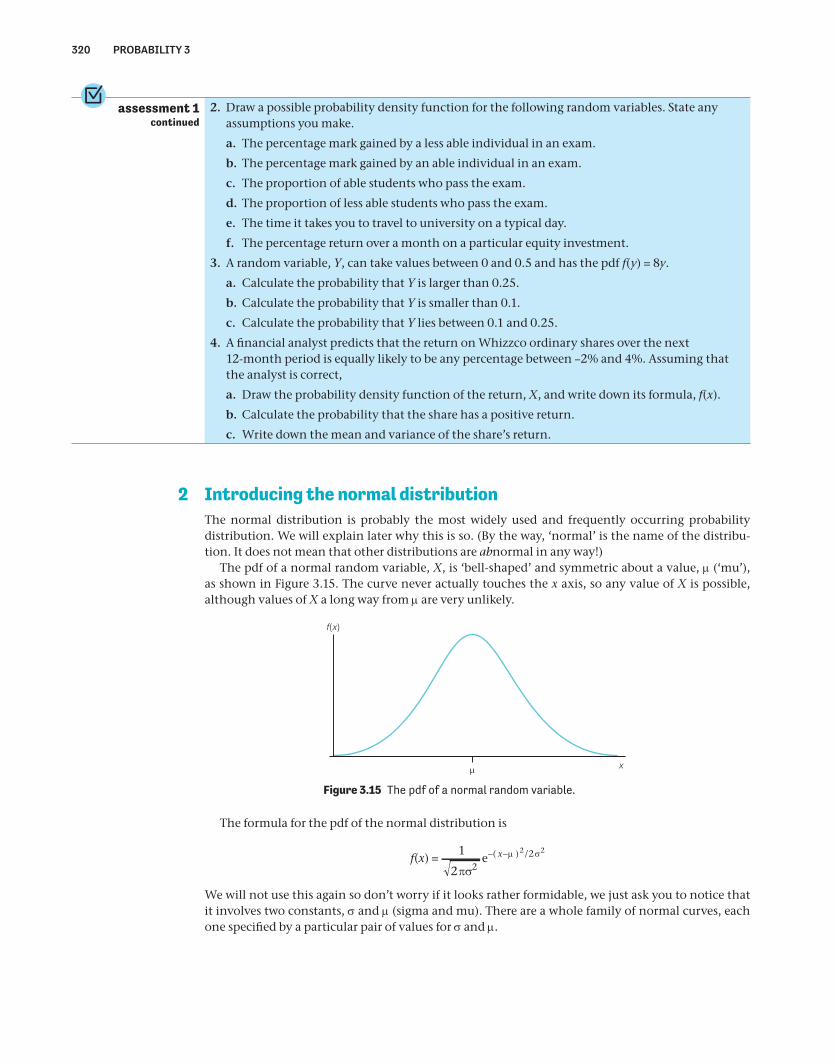
2. Draw a possible probability density function for the following random variables. State any assumptions you make.

a. The percentage mark gained by a less able individual in an exam.

b. The percentage mark gained by an able individual in an exam.

c. The proportion of able students who pass the exam.

d. The proportion of less able students who pass the exam.

e. The time it takes you to travel to university on a typical day.

f. The percentage return over a month on a particular equity investment.

3. A random variable, Y, can take values between 0 and 0.5 and has the pdf f( y) = 8y.

a. Calculate the probability that Y is larger than 0.25.

b. Calculate the probability that Y is smaller than 0.1.

c. Calculate the probability that Y lies between 0.1 and 0.25.

4. A fi nancial analyst predicts that the return on Whizzco ordinary shares over the next 12-month period is equally likely to be any percentage between –2% and 4%. Assuming that the analyst is correct,

a. Draw the probability density function of the return, X, and write down its formula, f(x).

b. Calculate the probability that the share has a positive return.

c. Write down the mean and variance of the share’s return.

2 Introducing the normal distributionThe normal distribution is probably the most widely used and frequently occurring probability distribution. We will explain later why this is so. (By the way, ‘normal’ is the name of the distribu-tion. It does not mean that other distributions are abnormal in any way!)

The pdf of a normal random variable, X, is ‘bell-shaped’ and symmetric about a value, (‘mu’), as shown in Figure 3.15. The curve never actually touches the x axis, so any value of X is possible, although values of X a long way from are very unlikely.

x

f(x)

Figure 3.15 The pdf of a normal random variable.

The formula for the pdf of the normal distribution is

f(x) =1

2 222 2

e ( ) /x

We will not use this again so don’t worry if it looks rather formidable, we just ask you to notice that it involves two constants, and (sigma and mu). There are a whole family of normal curves, each one specifi ed by a particular pair of values for and .

320 PROBABILITY 3

Both and have a ‘nice’ interpretation. We have already said that the pdf is symmetric about , so it is no surprise that is the mean of the distribution. The other constant, , dictates how spread out and fl at the ‘bell-shape’ is, and in fact 2 is the variance of the normal distribution. As an illustration, Figure 3.16 shows the following normal pdfs:

A = 10, = 1B = 10, = 2C = 10, = 3D = 15, = 1

A

B

C

x151050

f (x ) D

Figure 3.16 Some normal pdfs.

Pdfs A, B and C all have the mean 10, so they are all centred at x = 10. Of these three curves, C has the largest variance and so is the most ‘spread out’. Curve B has a smaller variance and so is less spread out, and curve A has the smallest variance and so is the most ‘squeezed in’. Curves A and D have the same variance, so they have exactly the same shape, but they have different means so they are centred at x = 10 and x = 15 respectively.

Some notation

As the normal distribution is entirely specifi ed by its mean and variance, a shorthand notation has been developed. X ~ N(, 2) means that the random variable X has a normal distribution with mean and variance 2. So, for instance, the curve shown in A above is the pdf of a N(10,1) distribution, the curve in B is the pdf of a N(10,4) distribution and so on.

The standard normal distribution

The normal distribution with mean = 0 and variance 2 = 1, is called the standard normal distri-bution. The letter Z is usually used for a random variable that has this distribution. A graph of the standard normal pdf, (z), is shown in Figure 3.17. Notice that most of the area under the standard normal curve lies between –3 and +3.

–4z

(z)

–3 –2 –1 10 2 3 4

Figure 3.17 The pdf of the standard normal distribution.


P

When does the normal distribution arise?

Because the normal pdf peaks at the mean and ‘tails off’ towards the extremes, the normal distribu-tion provides a good approximation for many naturally occurring random variables. However, the normal distribution occurs even more widely for the following reasons.

1. The total (and also the average) of a large number of random variables that have the same probability distribution has an approximately normal distribution. For instance, if the amount taken by a shop in a day has a particular (maybe unknown) probability distribution, the total of 100 days’ takings is the sum of 100 identically distributed random variables and so it will (approx-imately) have a normal distribution.

Many random variables are normal because of this. For example, the amount of rainfall that falls during a month is the total of the amounts of rainfall that have fallen each day or each hour of the month and so is likely to have a normal distribution. In the same way the average or total of a large sample will usually have a normal distribution. This will be important when we consider populations and samples in the Statistics part of this book.

2. The normal distribution provides approximate probabilities for a distribution called the binomial distribution, which we consider in P4, section 1.

Calculating probabilities: the standard normal distribution

The normal distribution is continuous and so its probabilities are calculated by obtaining the areas under the pdf curve.

For instance, suppose individuals’ IQ scores, X, have a normal distribution with mean = 100 and standard deviation = 15. As the standard deviation is 15 we can write this

X ~ N(100, 152) or equivalently X ~ N(100, 225).

Figure 3.18 shows the areas under the pdf that correspond to P(X < 85) and P(115 < X < 120).

x120

1301151008570

P(X < 85)

f(x )

P(115 < X < 120)

Figure 3.18

Unfortunately, there are no ‘nice’ formulae for calculating such areas so we have to look them up in tables of normal probabilities or use statistical software.

Using tables to calculate standard normal probabilities

We will start by evaluating probabilities for a standard normal random variable. This may not seem very useful, but in fact such probabilities form the basis of the calculation of all normal probabilities, as we shall see in the next section.

Standard normal probabilities of the form P(Z < a) are listed in a table of cumulative normal proba-bilities such as Table II at the end of this book (pp. 688–689). A section of Table II is shown opposite.

322 PROBABILITY 3

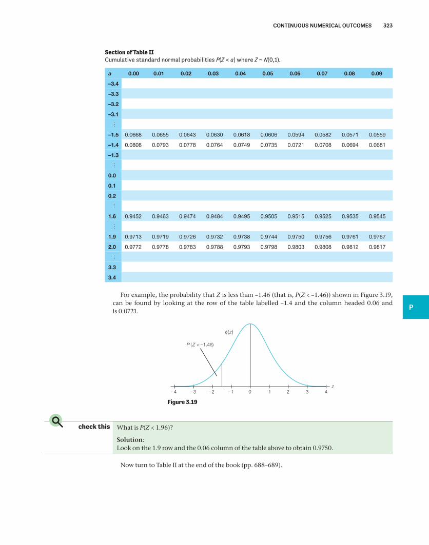
For example, the probability that Z is less than –1.46 (that is, P(Z < –1.46)) shown in Figure 3.19, can be found by looking at the row of the table labelled –1.4 and the column headed 0.06 and is 0.0721.

– 4 – 3 –2 –1

(z

z

)

P ( Z < –1.46)

10 2 3 4

Figure 3.19

check this What is P(Z < 1.96)?

Solution:Look on the 1.9 row and the 0.06 column of the table above to obtain 0.9750.

Now turn to Table II at the end of the book (pp. 688–689).

Section of Table II Cumulative standard normal probabilities P(Z < a) where Z ~ N(0,1).

a 0.00

–3.4

–3.3

–3.2

–3.1

–1.5 0.0668 0.0655 0.0643 0.0630 0.0618 0.0606 0.0594 0.0582 0.0571 0.0559

–1.4 0.0808 0.0793 0.0778 0.0764 0.0749 0.0735 0.0721 0.0708 0.0694 0.0681

–1.3

0.0

0.1

0.2

1.6 0.9452 0.9463 0.9474 0.9484 0.9495 0.9505 0.9515 0.9525 0.9535 0.9545

1.9 0.9713 0.9719 0.9726 0.9732 0.9738 0.9744 0.9750 0.9756 0.9761 0.9767

2.0 0.9772 0.9778 0.9783 0.9788 0.9793 0.9798 0.9803 0.9808 0.9812 0.9817

3.3

3.4

0.01 0.02 0.03 0.04 0.05 0.06 0.07 0.08 0.09


P

check this Calculate P(Z < – 0.52).

Solution:

Look on the –0.5 row and the 0.02 column, to obtain 0.3015.

Probabilities of the form P(Z > a) or P(a < Z < b) can be calculated by expressing them in terms of the cumulative probabilities P(Z < a) given in Table II. It usually helps to draw a rough sketch of the standard normal pdf and mark the appropriate areas.

check this Use the section of Table II to calculate P(Z > 2.05).

Solution:

A sketch is shown in Figure 3.20.

–4 –3 –2 –1

(z

z

)

P (Z > 2.05)

10 2 3 4

Figure 3.20

P(Z > 2.05) is the area under the whole pdf (which is 1) less the area to the left of 2.05, i.e. it is 1 – P(Z < 2.05). From the section of Table II, P(Z < 2.05) = 0.9798, so P(Z > 2.05) = 0.0202.

check this Use the section of Table II to calculate P(Z > –1.52).

Solution:We require 1 – P(Z < –1.52) = 1 – 0.0643 = 0.9357.

check this Use Table II itself to calculate P(–1.96 < Z < 1.25).

Solution:

The required probability is shown in Figure 3.21.

z1.250–1.96

P (–1.96 < Z < 1.25)

( )z

Figure 3.21

It is the area to the left of 1.25, P(Z < 1.25), less the area to the left of –1.96, P(Z < –1.96); that is, P(–1.96 < Z < 1.25) = P(Z < 1.25) – P(Z < –1.96) = 0.8944 – 0.0250 = 0.8694 from Table II.

324 PROBABILITY 3

Calculating percentage points

Sometimes we will know a cumulative probability but require the corresponding value of Z. For instance, suppose we need to fi nd the value a such that P(Z < a) = 0.95, as shown in Figure 3.22.

az

0

0.95

(z )

Figure 3.22

There are two ways to fi nd a. First, we can use the table of cumulative normal probabilities, Table II, in reverse. The body of the table contains P(Z < a) so we need to fi nd 0.95 in the body of the table and then look at the margins to see which value of a this corresponds to. On inspection, 0.95 does not explicitly appear in the body of the table – the entry for 1.64 is 0.9495 and the entry for 1.65 is 0.9505. It therefore seems a reasonable guess to suppose that the value we seek lies midway between 1.64 and 1.65. We conclude that P(Z < 1.645) = 0.95, although using the mid-point is an approximation.

The second way avoids this approximation and is the recommended method. Tables of inverse normal probabilities or normal percentage points, such as the one in Table III (pp. 690–691), give the value of a that corresponds to a particular cumulative probability, p. An extract from Table III is given below.

Section of Table III

Percentage points of the standard normal distributionThe table gives values of a, where P(Z < a) = p

p 0.000

0.00 –3.0902 –2.8782 –2.7478 –2.6521 –2.5758 –2.5121 –2.4573 –2.4093 –2.3656

0.01

0.02

0.03

0.10 –1.2816 –1.2759 –1.2702 –1.2646 –1.2591 –1.2536 –1.2481 –1.2426 –1.2372 –1.2319

0.95 1.6449 1.6546 1.6646 1.6747 1.6849 1.6954 1.7060 1.7169 1.7279 1.7392

0.96

0.97

0.98

0.99 2.3263 2.3656 2.4089 2.4573 2.5121 2.5758 2.6521 2.7478 2.8782 3.0902

0.001 0.002 0.003 0.004 0.005 0.006 0.007 0.008 0.009

To fi nd a such that P(Z < a) = 0.95 using this table, we look in the row for 0.95, and, as the third decimal place of 0.95 is zero, the column corresponding to 0.000. This gives a = 1.6449, so we conclude that P(Z < 1.6449) = 0.95.

The value of a random variable that corresponds to a cumulative probability of p is called the 100p th percentage point or the 100p th percentile. So we have just found that the 95th percentage point (or 95th percentile) of the standard normal distribution is 1.6449. We will not use this terminology very much but you may well encounter it elsewhere.


P

check this Find a such that P(Z < a) = 0.958.

Solution:

From the p = 0.95 row of the extract from Table III, and the 0.008 column we obtain a = 1.7279.

check this The return on a particular ordinary share is known to have a standard normal distribution. What value is such that the probability of a smaller return is 11%?

Solution:

We require a such that P(Z < a) = 0.11, shown in Figure 3.23.

za 0

0.11

( z)

Figure 3.23The entry at the intersection of the 0.11 row and the 0.000 column of Table III is –1.2265; that is, P(Z < –1.2265) = 0.11 and a = –1.2265. (We could also have used the cumulative probability table (Table II) in reverse and searched for 0.11 in the body of the table but this would have given the less accurate result that a is somewhere between –1.22 and –1.23.)

A dodge for calculating normal probabilities

There is a ‘dodge’ for calculating normal probabilities that is worth pointing out because it can save time.

As the standard normal distribution is symmetric about 0, the area under the pdf in the left-hand ‘tail’, P(Z < –a), is the same as the area under the pdf in the right-hand tail, P(Z > a), as shown in Figure 3.24.

a– a 0

P(Z –a )P(Z a)

( z

z

)

<>

Figure 3.24

check this What is P(Z > 1.3)?

Solution:

This is the area under the normal curve to the right of 1.3 so we cannot look it up in Table II immediately; we would have to calculate 1 – P(Z < 1.3). However, it is quicker to say that P(Z > 1.3) = P(Z < –1.3) which, from Table II, is 0.0968.

326 PROBABILITY 3

check this What is P(Z > –0.2)?

Solution:

P(Z > –0.2) is equivalent to P(Z < 0.2) as illustrated in Figure 3.25.

z–0.2 0

P(Z > –0.2)

z0.20

P(Z < 0.2)

( z )

( z )

Figure 3.25

From Table II, P(Z < 0.2) = 0.5793.

check this The deviation in mm between the diameter of a manufactured pipe and the specifi ed diameter can be positive or negative (or zero) and has a standard normal distribution. To be usable the diameter of a manufactured pipe must not differ from the specifi ed diameter by more than 2mm. What is the probability of an unusable pipe?

Solution:

We need the total of areas A1 (diameter too small) and A2 (diameter too large) shown in Figure 3.26 (not to scale).

z0–2

A1 A2

( z )

2

Figure 3.26

We could calculate each of these areas separately and then add them up. However, we know that P(Z < –2) and P(Z > 2) are the same, so we need only calculate one and then double the result. A1 = P(Z < –2) is obtained directly from Table II and is 0.0228. So the total area in both ‘tails’ is 2 × 0.0228 = 0.0456. We conclude that just under 5% of the pipes are not usable.


P

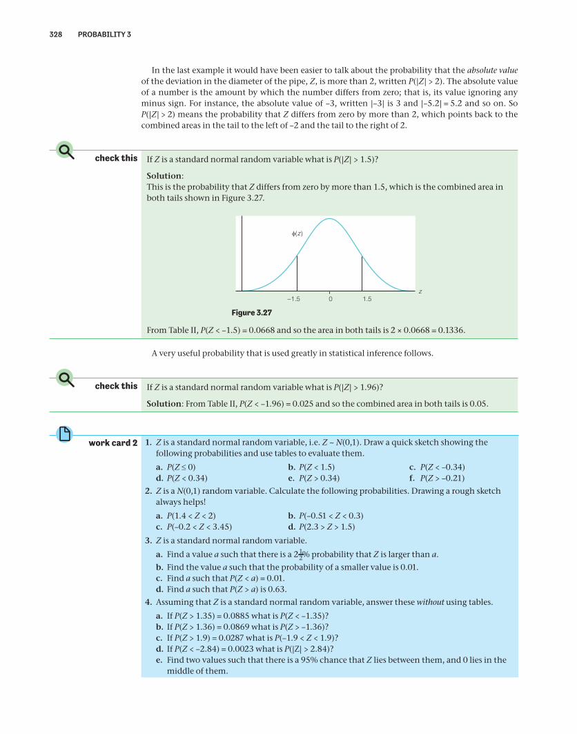
In the last example it would have been easier to talk about the probability that the absolute value of the deviation in the diameter of the pipe, Z, is more than 2, written P(|Z| > 2). The absolute value of a number is the amount by which the number differs from zero; that is, its value ignoring any minus sign. For instance, the absolute value of –3, written |–3| is 3 and |–5.2| = 5.2 and so on. So P(|Z| > 2) means the probability that Z differs from zero by more than 2, which points back to the combined areas in the tail to the left of –2 and the tail to the right of 2.

check this If Z is a standard normal random variable what is P(|Z| > 1.5)?

Solution:This is the probability that Z differs from zero by more than 1.5, which is the combined area in both tails shown in Figure 3.27.

0–1.5

( z

z

)

1.5

Figure 3.27

From Table II, P(Z < –1.5) = 0.0668 and so the area in both tails is 2 × 0.0668 = 0.1336.

A very useful probability that is used greatly in statistical inference follows.

check this If Z is a standard normal random variable what is P(|Z| > 1.96)?

Solution: From Table II, P(Z < –1.96) = 0.025 and so the combined area in both tails is 0.05.

work card 2 1. Z is a standard normal random variable, i.e. Z ~ N(0,1). Draw a quick sketch showing the following probabilities and use tables to evaluate them.

a. P(Z 0) b. P(Z < 1.5) c. P(Z < –0.34)d. P(Z < 0.34) e. P(Z > 0.34) f. P(Z > –0.21)

2. Z is a N(0,1) random variable. Calculate the following probabilities. Drawing a rough sketch always helps!

a. P(1.4 < Z < 2) b. P(–0.51 < Z < 0.3)c. P(–0.2 < Z < 3.45) d. P(2.3 > Z > 1.5)

3. Z is a standard normal random variable.

a. Find a value a such that there is a 212% probability that Z is larger than a.

b. Find the value a such that the probability of a smaller value is 0.01.c. Find a such that P(Z < a) = 0.01.d. Find a such that P(Z > a) is 0.63.

4. Assuming that Z is a standard normal random variable, answer these without using tables.

a. If P(Z > 1.35) = 0.0885 what is P(Z < –1.35)?b. If P(Z > 1.36) = 0.0869 what is P(Z > –1.36)?c. If P(Z > 1.9) = 0.0287 what is P(–1.9 < Z < 1.9)?d. If P(Z < –2.84) = 0.0023 what is P(|Z| > 2.84)?e. Find two values such that there is a 95% chance that Z lies between them, and 0 lies in the

middle of them.

328 PROBABILITY 3


Solutions:

1. a. You can do this one without tables because z = 0 is the half-way point of a symmetric distribution so P(Z 0) = 0.5.

b. P(Z < 1.5) = 0.9332.c. P(Z < –0.34) = 0.3669.d. P(Z < 0.34) = 0.6331.e. P(Z > 0.34) = 1 – P(Z < 0.34) = 1 – 0.6331 = 0.3669 or use (Z > 0.34) = P(Z < –0.34) = 0.3669

from c.f. P(Z > –0.21) = 1 – P(Z < –0.21) = 1 – 0.4168 = 0.5832.

2. a. P(1.4 < Z < 2) = P(Z < 2) – P(Z < 1.4) = 0.9772 – 0.9192 = 0.0580.b. P(–0.51 < Z < 0.3) = P(Z < 0.3) – P(Z < –0.51) = 0.6179 – 0.3050 = 0.3129.c. P(–0.2 < Z < 3.45) = P(Z < 3.45) – P(Z < –0.2) = 0.9997 – 0.4207 = 0.579.d. P(2.3 > Z > 1.5) = P(Z < 2.3) – P(Z < 1.5) = 0.9893 – 0.9332 = 0.0561.

3. Use Table III (or, less accurately, look up the probability in the body of Table II).

a. P(Z < a) = 0.975, so look up p = 0.975 in Table III to give a = 1.96.b. –2.3263.c. Same as b.d. If P(Z > a) = 0.63 it follows that P(Z < a) = 0.37. Looking up p = 0.37 in Table III gives

a = –0.3319.

4. a. P(Z < –1.35) is identical to P(Z > 1.35) so it too is 0.0885.b. A graph is recommended here. P(Z > –1.36) = 1 – P(Z < –1.36), and P(Z < –1.36) is the same as

P(Z > 1.36), so the answer is 1 – 0.0869 = 0.9131.c. P(–1.9 < Z < 1.9) is the entire area under the normal pdf less the area in each of the two

‘tails’, P(Z < –1.9) and P(Z > 1.9). Each tail has the same area of 0.0287 so the answer is 1 – (2 0.0287) = 0.9426.

d. P(|Z| > 2.84) means the probability that Z differs from 0 by more than 2.84 and so is the combined area in both tails, 2 0.0023 = 0.0046.

e. As 0 must lie in the middle, the lower and upper values must be –a and +a, respectively, so the tail areas to the left of –a and right of a are the same. As we require the area under the pdf between the two values to be 0.95, the area in each tail must be 0.025, so P(Z < – a) = 0.025. Using tables, a = 1.96, so the two values are –1.96 and 1.96.

assessment 2 1. Calculate the following probabilities when Z is a N(0,1) random variable.

a. P(Z < 1.32)b. P(Z < –1.32)c. P(Z > 2.25)d. P(Z < – 4.1).

2. In all the following questions Z is a standard normal random variable.

a. 0.18 is the probability that a standard normal random variable is less than what value?b. Find a when P(Z < a) = 0.18.c. Find a such that P(Z > a) = 0.76.d. For what value is the probability that Z exceeds it, 6%?

3. When Z is a standard normal random variable P(Z < –1.5) = 0.0668. Deduce the following without using tables.

a. P(Z > 1.5)b. P(Z > –1.5)c. P(–1.5 < Z < 1.5)d. P(|Z| > 1.5)


P

3 Calculating normal probabilitiesWe will now see that any normal probability can be expressed in terms of a standard normal proba-bility.

Standardising

Any normal random variable, X, that has mean and variance 2 can be standardised as follows.Take the variable X, and

(i) subtract its mean, , and then(ii) divide by its standard deviation, .

We will call the result Z, so

ZX

For example, suppose that X is individuals’ IQ scores and that it has a normal distribution with mean = 100 and standard deviation = 15, i.e. X ~ N(100,152). To standardise X we subtract = 100 and divide the result by = 15 to give

ZX 100

15

In this way, every value of X has a corresponding value of Z. For instance, when X = 130

Z130 100

152

and when X = 90

Z90 100

150 67.

Notice that Z is the number of standard deviations that X lies from its mean. So, for this example, an IQ of 130 is 2 standard deviations of 15 above the mean 100 and an IQ of 90 is 0.67 standard deviations of 15 below the mean.

check this The percentage monthly return on an ordinary share, X, has a normal distribution with mean 3 and variance 4. How would you calculate the standardised return?

In a particular month the return is X = 6. Standardise this and say how many standard deviations it is above or below the mean.

Solution:

To standardise we subtract the mean and divide by the standard deviation so the standardised return would be

ZX 3

2

When X = 6,

Z6 3

215.

and X = 6 is 1.5 standard deviations above the mean.

330 PROBABILITY 3

The distribution of standardised normal random variables

The reason for standardising a normal random variable in this way is that:a standardised normal random variable

ZX

has a standard normal distribution. That is,

ZX

N~ ( , )0 1

Another way of saying this is that the number of standard deviations that a normal random variable is away from its mean has a standard normal distribution. So if we take any normal random variable, subtract its mean and then divide by its standard deviation, the resulting random variable will have a standard normal distribution. We are going to use this fact to calculate (non-standard) normal probabilities.

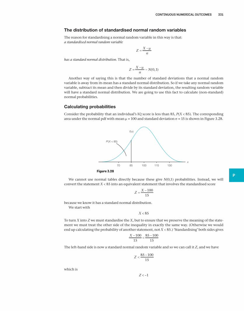
Calculating probabilities

Consider the probability that an individual’s IQ score is less than 85, P(X < 85). The corresponding area under the normal pdf with mean = 100 and standard deviation = 15 is shown in Figure 3.28.

x100 1158570

f (x)

P(X < 85)

130

Figure 3.28

We cannot use normal tables directly because these give N(0,1) probabilities. Instead, we will convert the statement X < 85 into an equivalent statement that involves the standardised score

ZX 100

15

because we know it has a standard normal distribution.We start with

X < 85

To turn X into Z we must standardise the X, but to ensure that we preserve the meaning of the state-ment we must treat the other side of the inequality in exactly the same way. (Otherwise we would end up calculating the probability of another statement, not X < 85.) ‘Standardising’ both sides gives

X 10015

85 10015

The left-hand side is now a standard normal random variable and so we can call it Z, and we have

Z85 100

15

which is

Z < –1


P

So, we have established that the statement we started with, X < 85, is equivalent to Z < –1. This means that whenever an IQ score, X, is less than 85 the corresponding standardised score, Z, will be less than –1, and so the probability we are seeking, P(X < 85), is the same as P(Z < –1).

P(Z < –1) is just a standard normal probability and so we can look it up in Table II in the usual way, which gives 0.1587. We conclude that P(X < 85) = 0.1587.

This process of rewriting a probability statement about X in terms of Z is not diffi cult if you are systematic and write down what you are doing at each stage. We would lay out the working we have just done for P(X < 85) as follows.

check this X has a normal distribution with mean 100 and standard deviation 15. What is the probability that X is less than 85?

Solution:

P(X < 85) = PX 100

1585 100

15P(Z < –1) = 0.1587 (from tables).

Try the following.

check this Assuming that an individual’s IQ score has a N(100,152) distribution, what is the probability that an individual’s IQ score is more than 125?

Solution:We require

P X PX

P Z( ) ( . )125100

15125 100

15167

Table II gives P(Z < 1.67) = 0.9525, so we have

P(Z > 1.67) = 1 – P(Z < 1.67) = 1 – 0.9525 = 0.0475.

check this For each of these write down the equivalent standard normal probability. (Don’t bother to look up the probability in Table II unless you are really keen!)

a. The IQ of randomly chosen university students, X, is normally distributed with mean 115 and standard deviation 10. Consider the probability that a student has an IQ of over 150.

b. The number of people who visit an historic monument in a week is normally distributed with a mean of 10,500 and a standard deviation of 600. Consider the probability that fewer than 9000 people visit in a week.

c. The number of cheques processed by a bank each day is normally distributed with a mean of 30,100 and a standard deviation of 2450. Consider the probability that the bank processes more than 32,000 cheques in a day.

Solutions:

a. P X PX

P Z( ) ( . )150115

10150 115

103 5

b. P X PX

P Z( ), ,

(900010 500600

9000 10 500600

2. )5

c. P X PX

( , ), , ,

32 00030 100

245032 000 30 100

2450P Z( . )0 78

332 PROBABILITY 3

check this A fl ight is due at Heathrow airport at 1800 hours. Its arrival time has a normal distribution with mean 1810 hours and standard deviation 10 minutes.

a. What is the probability that the fl ight arrives before its due time?b. Passengers must check-in for a connecting fl ight by 1830 at the latest. What is the probability

that passengers from the fi rst fl ight arrive too late for the connecting fl ight? (Assume no travelling time from aircraft to check-in.)

Solution:

Let the time of arrival, in minutes past 1800, be X, so X ~ N(10,102).

a. We require

P X PX

P Z( ) ( ) .010

100 10

101 0 1587

b. P X PX

P Z( ) ( ) .3010

1030 10

102 0 0228

Probabilities like P(a < X < b) can be calculated in the same way. The only difference is that when X is standardised similar operations must be applied to both a and b. That is, a < X < b becomes

a X b which is aZ

b

check this Individuals’ IQ scores have an N(100,152) distribution. What is the probability that an individual’s IQ score is between 91 and 121?

Solution: We require P(91 < X < 121). Standardising gives

PX91 100

15100

15121 100

15

The middle term is a standardised normal random variable and so we have

P Z P Z9

152115

0 6 14 0 9192 0 2743 0 6( . . ) . . . 449

check this For each of these write down the equivalent standard normal probability.

a. The length of metallic strips produced by a machine has mean 100 cm and variance 2.25 cm. Only strips with a length between 98 and 103 cm are acceptable. What is the probability that a metallic strip has an acceptable length? You may assume that the length of a strip has a normal distribution.

b. Scores in an exam are adjusted so that they have a normal distribution with an average mark of 56 and a standard deviation of 12. Students gaining between 40 and 70 are considered ‘mainstream’. Consider the probability that a student gains a ‘mainstream’ score.

Solutions:

a. X ~ N(100,2.25) so P(98 < X < 103)

PX

P Z98 100

15100

15103 100

15133

. . .( . 2)

b. X ~ N(56,122) so P(40 < X < 70)

PX

P Z40 56

1256

1270 56

12133 117( . . )


P

Calculating percentage points

Sometimes you will know a probability but want to calculate the corresponding value of X. For instance, you may need to fi nd the value a such that P(X < a) = 0.95. Again we can do this by chang-ing the statement X < a into an equivalent statement about Z by standardising X.

check this The random variable X is normally distributed with mean 20 and variance 16. What value of X is such that the probability that X is smaller is 35%?

Solution:X ~ N(20,16) and we require a such that P(X < a) = 0.35 as shown in Figure 3.29a.

a 20

f (x

x

)

0.35

Figure 3.29a

We know P(X < a) = 0.35. Standardising this gives

PX a20

420

40 35.

X 204 is a standardised normal random variable, Z, so our problem is now to fi nd a such that

P Za 20

40 35.

as shown in Figure 3.29b.

z

0.35

a – 204

( z )

Figure 3.29b

When we look up 0.35 in Table III we obtain –0.3853; that is, P(Z < –0.3853) = 0.35. So, it follows that

a 204

0 3853.

Solving this for a gives a = (4 × –0.3853) + 20 = 18.4588.So the probability that X is less than 18.4588 is 35%.

334 PROBABILITY 3

check this According to a survey, dentists’ salaries have an average of £48,000 with a standard deviation of £3500. If the salary of a dentist is normally distributed, what salary is such that 20% of dentists have a higher salary?

Solution:

We require a such that P(X > a) = 0.2. We will work in £1000s.

X ~ N(48,3.52)

so standardising

P(X > a) = 0.2

gives

PX a48

3 548

3 50 2

. ..

that is

P Za 48

3 50 2

..

as shown in Figure 3.30.

0.2

a – 483.5

( z

z

)

Figure 3.30

It follows that

P Za 48

3 50 8

..

and looking up 0.8 in Table III gives

P(Z < 0.8416) = 0.8

So

a 483 5

0 8416.

.

and solving for a gives a = 50.9456.We conclude that 20% of dentists earn more than £50,946.


P

check this The amount a customer spends on a single visit to Rainsburys supermarkets has a normal distribution with mean £75 and standard deviation £21. Rainsburys wish to introduce a minimum amount for which credit cards may be used – an amount which enables 80% of customers to pay by credit card. At what fi gure should this credit card minimum be set?

Solution:

We require a such that P(X > a) = 0.8, where X ~ N(75,212)

Standardising gives

PX a75

2175

210 8.

which is

P Za 75

210 8.

which is equivalent to

P Za 75

210 2.

Using Table III gives P(Z < –0.8416) = 0.2, so we have

a 7521

0 8416.

Solving for a gives a = (21 × –0.8416) + 75 = £57.3264.The credit card minimum should be set at £57.33.

Normal probabilities using software

Most statistical software can calculate cumulative normal probabilities P(X < a) and percentage points (which some software call the inverse cumulative probabilities).

Use SPSS’sTransform > Compute Variable

command and then select the CDF.NORMAL function in order to calculate the cumulative normal probability. You will need to specify the values for a, the mean and the standard deviation. For instance, when X ~ N(75,212) CDF.NORMAL gives P(X < 50) = 0.1169.

We can fi nd percentage points by selecting the IDF.NORMAL function. For the same distribu-tion, we fi nd that the 20th percentage point is 57.3260. This result differs slightly from our earlier manual calculation because the values in Table III are given to only 4 d.p., whereas SPSS’s algorithm retains more decimal places in its calculations and so is more accurate.

In Microsoft® Excel you need the function NORM.DIST to calculate normal and cumulative normal probabilities, and NORM.INV to calculate the inverse cumulative probability (NORMDIST and NORMINV for Excel 2007 and earlier).

work card 3 1. X is a normal random variable with mean = 5 and variance 2 = 4. Calculate the following probabilities:

a. P(X > 5.7) b. P(X < 3.4)c. P(2.8 < X < 5.1) d. P(5.7 < X < 6.8)

2. X is normally distributed with mean 10 and variance 9. Find a such that:

a. the probability that X is less than a is 0.51b. P(X > a) = 0.6c. P(X a) = 0.05d. P(10 < X < a) = 0.05

336 PROBABILITY 3

work card 3

continued overleaf

3. The yearly cost of dental claims for the employees of Notooth International is normally distributed with mean = £75 and standard deviation = £25. Using a computer or otherwise, fi nd:

a. What proportion of employees can be expected to claim over £120 in a year?b. What yearly cost do 30% of employees claim less than?

4. Petrol consumption for all types of small car is normally distributed with = 30.5 m.p.g. and = 4.5 m.p.g.

A manufacturer wants to make a car that is more economical than 95% of small cars. What must be its m.p.g? Use a computer if you want.

Solutions:

1. a. P(X > 5.7) = P(Z > 0.35) = 0.3632b. P(X < 3.4) = P(Z < –0.8) = 0.2119c. P(2.8 < X < 5.1) = P(–1.1 < Z < 0.05) = P(Z < 0.05) – P(Z < –1.1) = 0.5199 – 0.1357 = 0.3842d. P(5.7 < X < 6.8) = P(0.35 < Z < 0.9) = P(Z < 0.9) – P(Z < 0.35) = 0.8159 – 0.6368 = 0.1791

2. Sketches will help you here.a. P(X < a)

PX a

P Za10

310

310

3051.

Using tables P(Z < 0.0251) = 0.51, so

a 103

0 0251. and a 10 0753.

b. P(X > a) = 0.6

PX a

P Za10

310

310

30 6.

Soa 10

30 2533. and a = 9.2401

c. P(X a)

PX a

P Za10

310

310

30 05.

Soa 10

316449. and a = 14.9347

d. P(10 < X < a)

PX a

P Za

P Za

10 103

103

103

010

310

30 0 05P Z( ) .

So P Za 10

30 5 0 05. . and P Z

a 103

0 55.

So a – 10 = 0.1257 and a = 10.3771

3. a. P(X > 120) = P(Z > 1.8) = 0.0359, so 3.59%.

b. We require a such that P(X < a) = 0.3, so

P Za 75

250.3,

a 7525

0.5244 and a 61.89

30% of employees claim less than £61.89.


P


4. We require a such that P(X < a) = 0.95, so

P Za 30 5

4 50 95

..

. , soa 30 5

4 516449

..

.

and a = 37.90205. 95% of small cars do less than 37.9 m.p.g.

assessment 3 1. X is a normal random variable with mean = –2 and variance 2 = 0.5. Calculate the following:

a. P(X < –3.5)b. P(X > 0)c. P(–1.5 < X < –0.8)

2. Calculate the following when X ~ N(100,64):

a. P(X > 120)b. P(X 99)c. P(90 < X < 100)

3. X has a normal distribution with mean = 4 and standard deviation = 1.5. Find a when P(4 – a < X < 4 + a) = 0.8.

4. The duration of a scheduled fl ight is normally distributed with a mean of 45 minutes and a standard deviation of 2 minutes.

a. What is the probability that the fl ight takes less than 42 minutes?b. What is the probability that it takes between 40 and 50 minutes?c. What times do 5% of fl ights take longer than?

5. For a particular life insurance policy the lifetime of the policyholders follows a normal distribution with mean 72.2 years and standard deviation 4.4 years. One of the options of this policy is that the policyholder receives a payment on their 70th birthday and another payment every 5 years thereafter.

a. What percentage of policyholders will receive at least one payment?b. What percentage will receive two or more?

Now, how about trying the set of multiple choice questions for this chapter on the companion website at

www.palgrave.com/companion/Swift-Quantitative-Methods-4

where you can also fi nd other additional resources.

338 PROBABILITY 3

3 Continuous Numerical outcomes - macmillanihe.com resources (by Author)/S... · The reason is that...

Documents

Transcript of 3 Continuous Numerical outcomes - macmillanihe.com resources (by Author)/S... · The reason is that...