Lecture Notes for AST 5622Astrophysical Dynamics

Prepared by

Dr. Joseph M. Hahn

Saint Mary’s University

Department of Astronomy & Physics

January 9, 2006

The Three–Body Problem

This lecture is drawn from M&D, Chapter 3.

The simplest 3–body problem is the restricted 3–body problem (R3BP):

this is the study of the motion of

a massless particle P (also called a test particle)

that is being perturbed by a secondary mass m2 (say, a planet)

that is in a circular orbit about a primary mass m1 (say, the Sun).

This problem is the easiest of all N–body problem where N > 2,

since the motion of the primary & secondary are known exactly.

However it is still challenging,

since there is no general analytic solution for particle P ’s motion.

This problem is most relevant to the study of the motion of small bodies

(ie, comets, asteroids, dust grains, etc) when they are perturbed by Jupiter

(which, by the way, has a small but non–zero eccentricity e = 0.05),

or by a ring particle that is perturbed by a satellite.

1

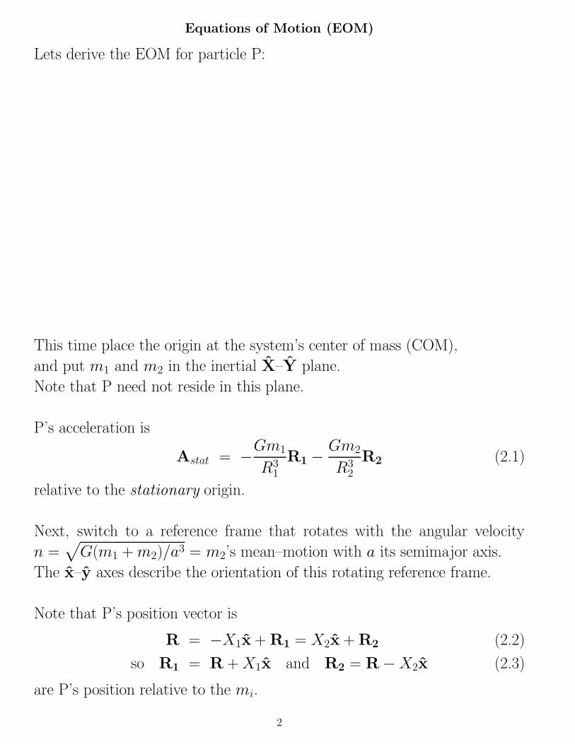
Equations of Motion (EOM)

Lets derive the EOM for particle P:

This time place the origin at the system’s center of mass (COM),

and put m1 and m2 in the inertial X–Y plane.

Note that P need not reside in this plane.

P’s acceleration is

Astat = −Gm1

R31

R1 −Gm2

R32

R2 (2.1)

relative to the stationary origin.

Next, switch to a reference frame that rotates with the angular velocity

n =√

G(m1 + m2)/a3 = m2’s mean–motion with a its semimajor axis.

The x–y axes describe the orientation of this rotating reference frame.

Note that P’s position vector is

R = −X1x + R1 = X2x + R2 (2.2)

so R1 = R + X1x and R2 = R − X2x (2.3)

are P’s position relative to the mi.

2

We want P’s acceleration measured in the rotating reference frame, Arot.

Recall from your classical mechanics class:

Arot = Astat − ~ω × (~ω × R) − 2~ω ×V (2.4)

where the middle & right terms are the centrifugal & Coriolis acceleration

that occur in this rotating reference frame,

~ω = nz is the rotation axis,

and V = dR/dt is P’s velocity measured in the rotating coordinate system.

(to refresh your memory, see page 8 of my PHY 3405 notes, posted at

http://apwww.stmarys.ca/∼jhahn/phy3405/2005fall/chap10.pdf)

The centrifugal acceleration is

Acent = −~ω × (~ω ×R) (2.5)

where ~ω ×R =

∣

∣

∣

∣

∣

∣

x y z

0 0 n

X Y Z

∣

∣

∣

∣

∣

∣

(2.6)

= −nY x + nXy (2.7)

so Acent = −~ω × (~ω ×R) =

∣

∣

∣

∣

∣

∣

x y z

0 0 −n

−nY nX 0

∣

∣

∣

∣

∣

∣

(2.8)

= n2Xx + n2Y y (2.9)

Similarly, the Coriolis acceleration is

Acor = −2~ω ×V =

∣

∣

∣

∣

∣

∣

x y z

0 0 −2n

X Y Z

∣

∣

∣

∣

∣

∣

(2.10)

= 2nY x − 2nXy (2.11)

so P’s acceleration in this rotating coordinate system is

R = Arot (2.12)

= −Gm1

R31

R1 −Gm2

R32

R2 + n2(Xx + Y y) + 2nY x − 2nXy (2.13)

3

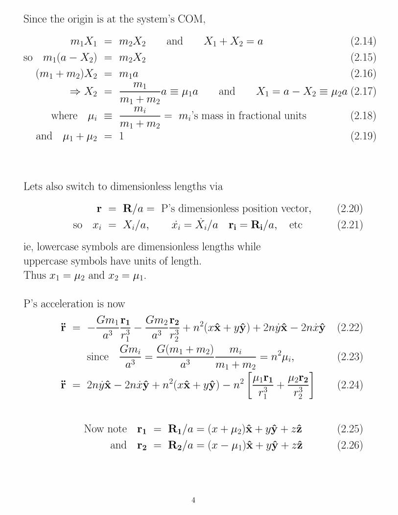
Since the origin is at the system’s COM,

m1X1 = m2X2 and X1 + X2 = a (2.14)

so m1(a − X2) = m2X2 (2.15)

(m1 + m2)X2 = m1a (2.16)

⇒ X2 =m1

m1 + m2

a ≡ µ1a and X1 = a − X2 ≡ µ2a (2.17)

where µi ≡ mi

m1 + m2

= mi’s mass in fractional units (2.18)

and µ1 + µ2 = 1 (2.19)

Lets also switch to dimensionless lengths via

r = R/a = P’s dimensionless position vector, (2.20)

so xi = Xi/a, xi = Xi/a ri = Ri/a, etc (2.21)

ie, lowercase symbols are dimensionless lengths while

uppercase symbols have units of length.

Thus x1 = µ2 and x2 = µ1.

P’s acceleration is now

r = −Gm1

a3

r1

r31

− Gm2

a3

r2

r32

+ n2(xx + yy) + 2nyx − 2nxy (2.22)

sinceGmi

a3=

G(m1 + m2)

a3

mi

m1 + m2

= n2µi, (2.23)

r = 2nyx − 2nxy + n2(xx + yy) − n2

[

µ1r1

r31

+µ2r2

r32

]

(2.24)

Now note r1 = R1/a = (x + µ2)x + yy + zz (2.25)

and r2 = R2/a = (x − µ1)x + yy + zz (2.26)

4

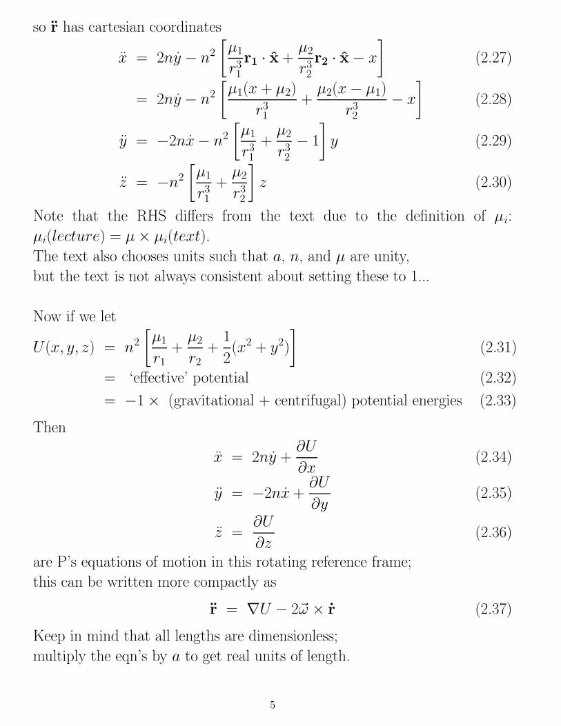
so r has cartesian coordinates

x = 2ny − n2

[

µ1

r31

r1 · x +µ2

r32

r2 · x − x

]

(2.27)

= 2ny − n2

[

µ1(x + µ2)

r31

+µ2(x − µ1)

r32

− x

]

(2.28)

y = −2nx − n2

[

µ1

r31

+µ2

r32

− 1

]

y (2.29)

z = −n2

[

µ1

r31

+µ2

r32

]

z (2.30)

Note that the RHS differs from the text due to the definition of µi:

µi(lecture) = µ × µi(text).

The text also chooses units such that a, n, and µ are unity,

but the text is not always consistent about setting these to 1...

Now if we let

U(x, y, z) = n2

[

µ1

r1

+µ2

r2

+1

2(x2 + y2)

]

(2.31)

= ‘effective’ potential (2.32)

= −1 × (gravitational + centrifugal) potential energies (2.33)

Then

x = 2ny +∂U

∂x(2.34)

y = −2nx +∂U

∂y(2.35)

z =∂U

∂z(2.36)

are P’s equations of motion in this rotating reference frame;

this can be written more compactly as

r = ∇U − 2~ω × r (2.37)

Keep in mind that all lengths are dimensionless;

multiply the eqn’s by a to get real units of length.

5

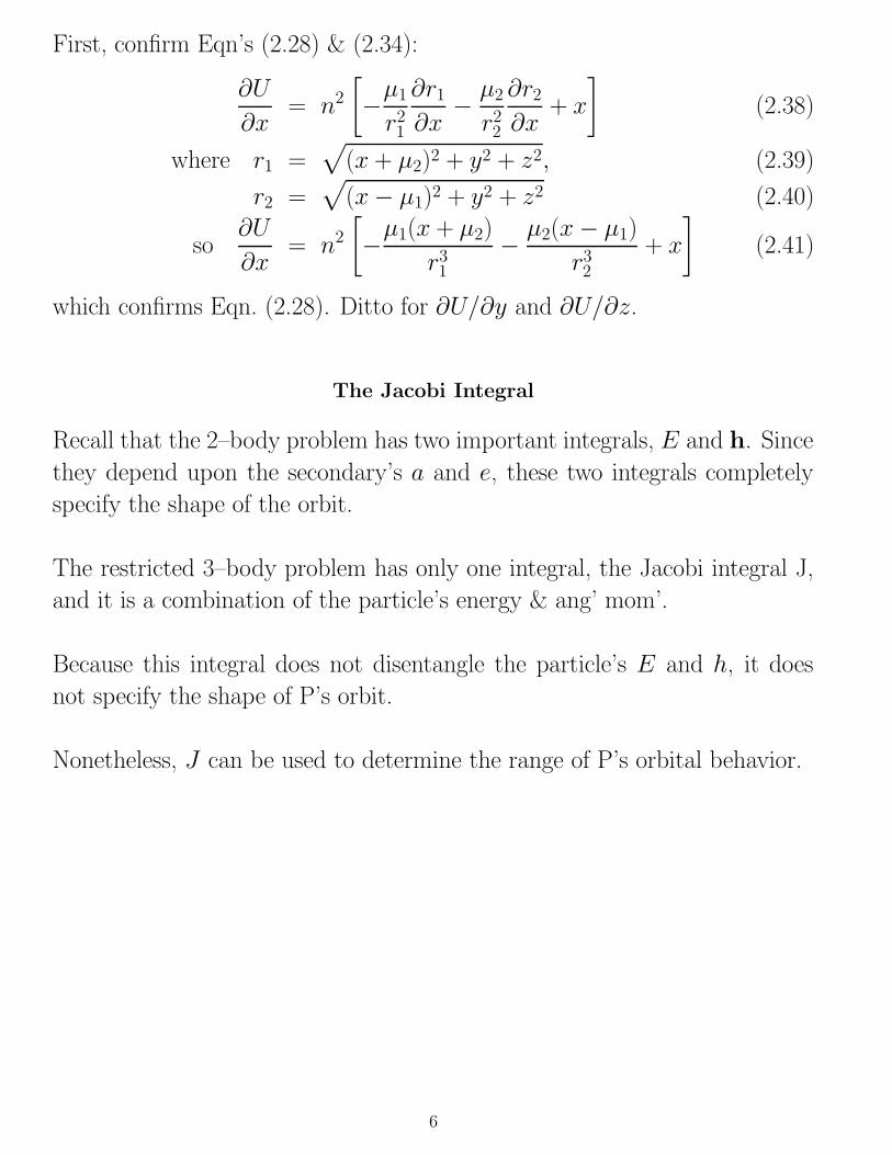
First, confirm Eqn’s (2.28) & (2.34):

∂U

∂x= n2

[

−µ1

r21

∂r1

∂x− µ2

r22

∂r2

∂x+ x

]

(2.38)

where r1 =√

(x + µ2)2 + y2 + z2, (2.39)

r2 =√

(x − µ1)2 + y2 + z2 (2.40)

so∂U

∂x= n2

[

−µ1(x + µ2)

r31

− µ2(x − µ1)

r32

+ x

]

(2.41)

which confirms Eqn. (2.28). Ditto for ∂U/∂y and ∂U/∂z.

The Jacobi Integral

Recall that the 2–body problem has two important integrals, E and h. Since

they depend upon the secondary’s a and e, these two integrals completely

specify the shape of the orbit.

The restricted 3–body problem has only one integral, the Jacobi integral J,

and it is a combination of the particle’s energy & ang’ mom’.

Because this integral does not disentangle the particle’s E and h, it does

not specify the shape of P’s orbit.

Nonetheless, J can be used to determine the range of P’s orbital behavior.

6

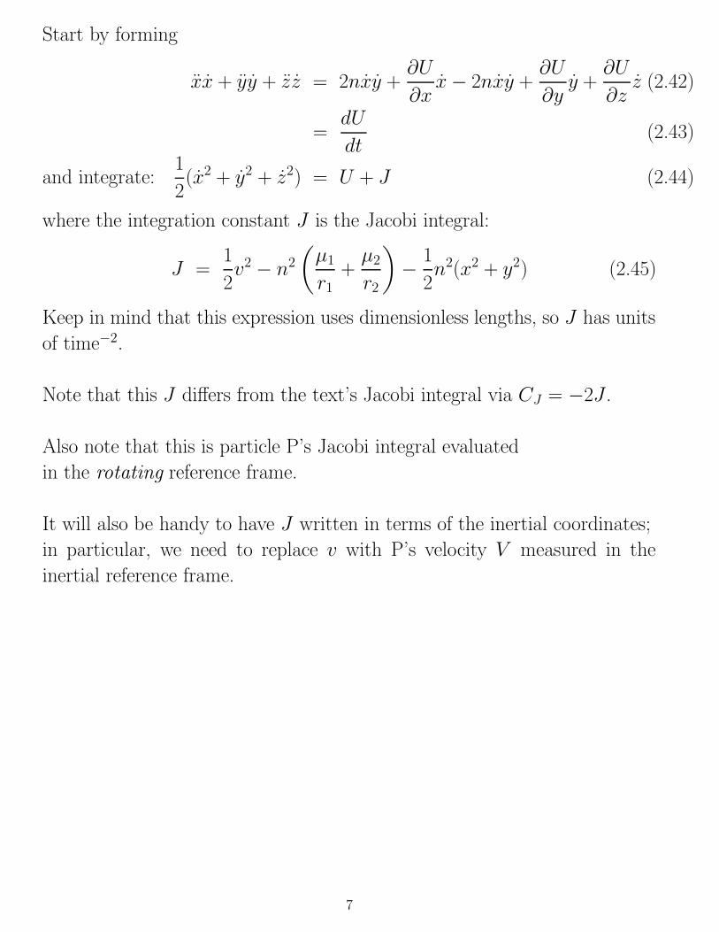
Start by forming

xx + yy + zz = 2nxy +∂U

∂xx − 2nxy +

∂U

∂yy +

∂U

∂zz (2.42)

=dU

dt(2.43)

and integrate:1

2(x2 + y2 + z2) = U + J (2.44)

where the integration constant J is the Jacobi integral:

J =1

2v2 − n2

(

µ1

r1

+µ2

r2

)

− 1

2n2(x2 + y2) (2.45)

Keep in mind that this expression uses dimensionless lengths, so J has units

of time−2.

Note that this J differs from the text’s Jacobi integral via CJ = −2J .

Also note that this is particle P’s Jacobi integral evaluated

in the rotating reference frame.

It will also be handy to have J written in terms of the inertial coordinates;

in particular, we need to replace v with P’s velocity V measured in the

inertial reference frame.

7

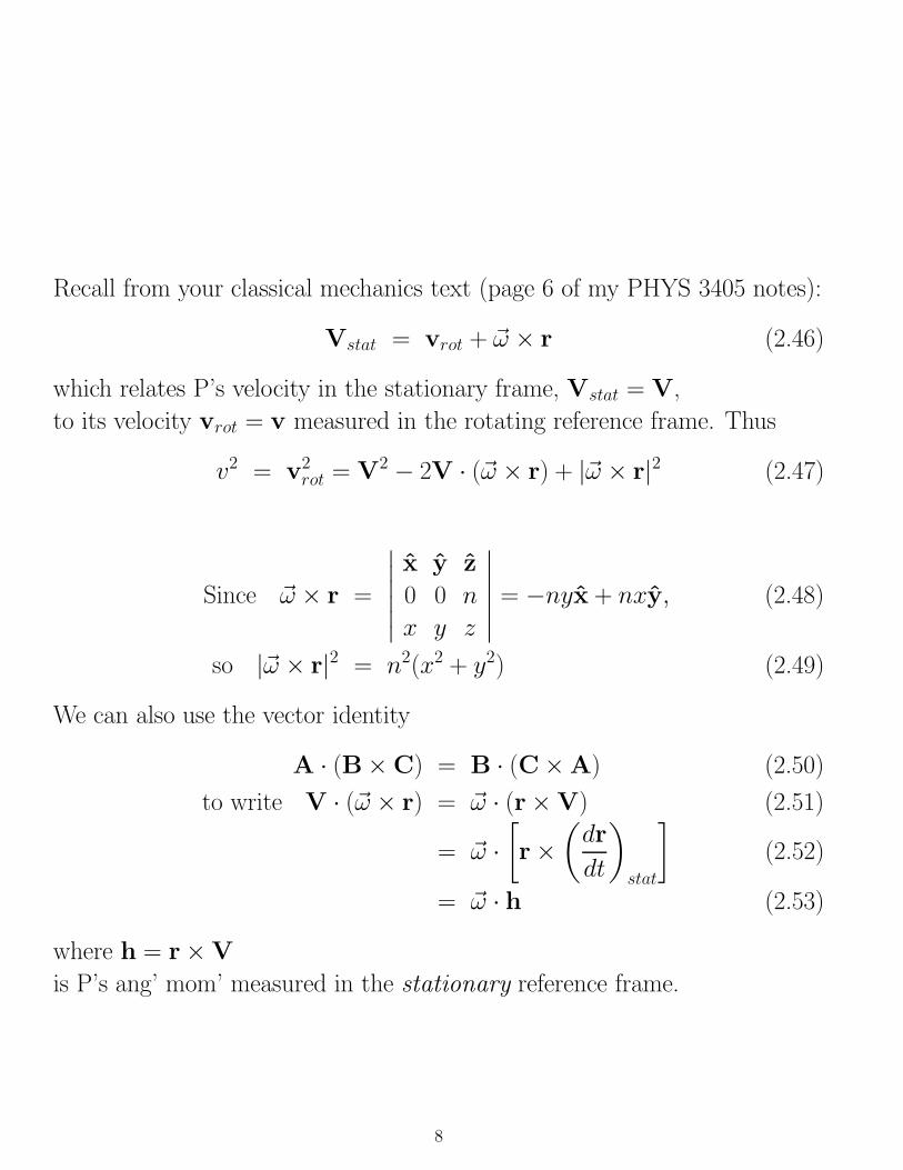
Recall from your classical mechanics text (page 6 of my PHYS 3405 notes):

Vstat = vrot + ~ω × r (2.46)

which relates P’s velocity in the stationary frame, Vstat = V,

to its velocity vrot = v measured in the rotating reference frame. Thus

v2 = v2rot = V2 − 2V · (~ω × r) + |~ω × r|2 (2.47)

Since ~ω × r =

∣

∣

∣

∣

∣

∣

x y z

0 0 n

x y z

∣

∣

∣

∣

∣

∣

= −nyx + nxy, (2.48)

so |~ω × r|2 = n2(x2 + y2) (2.49)

We can also use the vector identity

A · (B× C) = B · (C×A) (2.50)

to write V · (~ω × r) = ~ω · (r× V) (2.51)

= ~ω ·[

r ×(

dr

dt

)

stat

]

(2.52)

= ~ω · h (2.53)

where h = r × V

is P’s ang’ mom’ measured in the stationary reference frame.

8

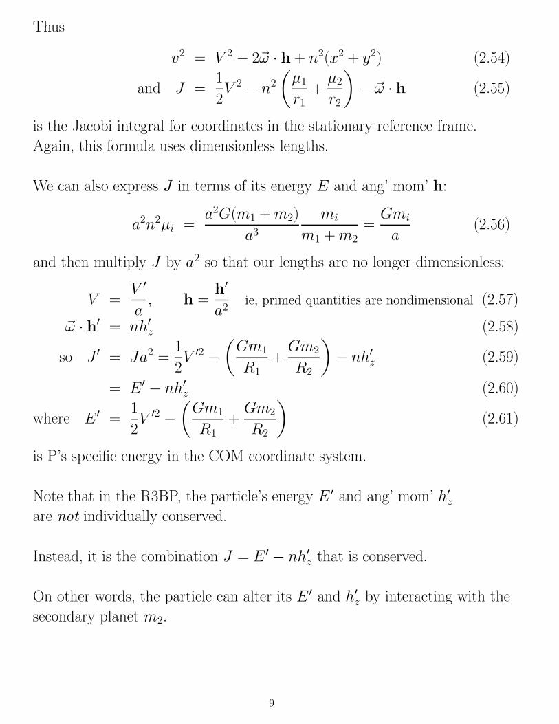
Thus

v2 = V 2 − 2~ω · h + n2(x2 + y2) (2.54)

and J =1

2V 2 − n2

(

µ1

r1

+µ2

r2

)

− ~ω · h (2.55)

is the Jacobi integral for coordinates in the stationary reference frame.

Again, this formula uses dimensionless lengths.

We can also express J in terms of its energy E and ang’ mom’ h:

a2n2µi =a2G(m1 + m2)

a3

mi

m1 + m2

=Gmi

a(2.56)

and then multiply J by a2 so that our lengths are no longer dimensionless:

V =V ′

a, h =

h′

a2ie, primed quantities are nondimensional (2.57)

~ω · h′ = nh′z (2.58)

so J ′ = Ja2 =1

2V ′2 −

(

Gm1

R1

+Gm2

R2

)

− nh′z (2.59)

= E ′ − nh′z (2.60)

where E ′ =1

2V ′2 −

(

Gm1

R1

+Gm2

R2

)

(2.61)

is P’s specific energy in the COM coordinate system.

Note that in the R3BP, the particle’s energy E ′ and ang’ mom’ h′z

are not individually conserved.

Instead, it is the combination J = E ′ − nh′z that is conserved.

On other words, the particle can alter its E ′ and h′z by interacting with the

secondary planet m2.

9

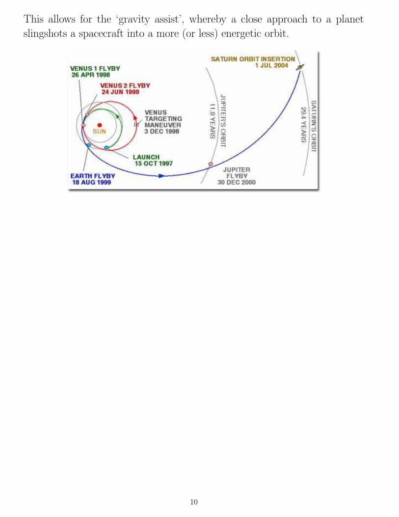
This allows for the ‘gravity assist’, whereby a close approach to a planet

slingshots a spacecraft into a more (or less) energetic orbit.

10

Osculating Orbital Elements

In the 2–body problem, m2’s orbit elements are constant.

But in the R3BP, particle’s P’s orbit elements a, e, i, Ω, ω, M are not

constants—they should be regarded as functions of time t that are known

as osculating orbit elements.

To calculate the osculating orbit elements at time t, you need to know P’s

position r(t) and velocity r(t) relative to the primary in the stationary

reference frame.

Then calculate P’s orbit elements assuming that P is the secondary, this

provides a, e, i, etc, for that instant of time t.

You can then use Kepler’s equation to calculate P’s r(t′) and r(t′)at other times t′.

However that of course will only yield an approximate solution for P’s

motion since that calculation ignores perturbations from any other planets,

stars, other forces, etc. The quality of this approximate solution will steadily

degrade over time.

An exact solution for P’s motion over time requires solving Newton’s laws

(usually numerically) in a manner that accounts for all other perturbing

forces.

11

some more Classical Mechanics

In my earlier review of classical mechanics,

I neglected to note a few other fundamental formulas:

1. We can usually write the force as F = −∇U ,

where U(r) is the system’spotential energy (or PE), and

∇U =∂U

∂xx +

∂U

∂yy +

∂U

∂zz in Cartesian coordinates (2.62)

=∂U

∂ρρ +

1

ρ

∂U

∂φφ +

∂U

∂zz in cylindrical coord’s (2.63)

2. For a particle of mass m, we call Φ(r) = U/m = m’s potential,

ie, its potential energy per unit mass.

Then by Newton’s 2nd law, m’s EOM is r = −∇Φ(r).

3. suppose the scalar function f = f(r, t) = f(x, y, z, t) is a function of the

spatial coordinate r and time t. Then by the Chain Rule,

df

dt=

∂f

∂x

dx

dt+

∂f

∂y

dy

dt+

∂f

∂z

dz

dt+

∂f

∂t= (∇f) · r +

∂f

∂t(2.64)

We will use this in the next homework.

12

A More General Derivation of J

The preceding derivation of the Jacobi integral J , which we was obtained

by considering the R3BP, is not the most general derivation.

Consider a particle that is subject to the potential Φ that is stationary (ie,

time-independent) in a reference frame that rotates with constant angular

velocity ω about some axis.

Does the potential experienced by the particle in the R3BP satisfy this

constraint?

In the following homework assignment, you will show that the particle also

has a conserved Jacobi integral

J = E − ~ω · L (2.65)

where E and L are the particle’s total energy and angular momenta mea-

sured in the inertial reference frame.

We will find this Jacobi integral very handy when we start studying the

motion of perturbed bodies, such as:

• a star in a galaxy that is disturbed by rotating central bar,

• or a particle disturbed by a planet in a circular orbit.

13

Assignment #2due Thursday February 2

at the start of class

1. Derive Eqn. (2.65) for a particle that is subject to a potential Φ that is

stationary in a reference frame that rotates at a constant angular velocity ω

about the rotation axis ~ω = ωz.

a.) Begin by writing the EOM for the particle’s position vector r in this

rotating reference frame. Then consider the product r · r to show that

d

dt

(

1

2r2 + Φ

)

= −[~ω × (~ω × r)] · r (2.66)

b.) identify the RHS with Eqn. (2.64) so that ∇f = −~ω × (~ω × r);

then verify that f = (~ω × r)2/2 satisfies the preceding result.

Tip: use cylindrical coordinates.

c.) use the above result to show that

J =1

2r2 + Φ − 1

2(~ω × r)2 (2.67)

is a constant of the motion. Keep in mind that r is the particle’s velocity in

the rotating reference frame.

d.) replace r with the particle’s velocity as measured in the inertial reference

frame, which then yields a jacobi integral

J = E − ~ω · L (2.68)

for a particle having specific energy and ang’ mom’ E and L.

14

3. Show that a dimensionless Jacobi integral,

J ′ =J

E2

=a

aP+ 2

√

(

1 +m2

m1

)

aP

a(1 − e2

P ) cos iP +m2

m1

a

R2

, (2.69)

when you write J in term’s of particle P’s osculating orbit elements

aP , eP , iP , where E2 is the secondary’s specific energy in the COM reference

frame.

4. The Tisserand parameter T is Eqn. (2.69) with the rightmost term

neglected, since that term is usually quite small. The Tisserand parameter

is useful in studies of cometary orbits, since it is approximately conserved in

a simple 1–planet system.

An active comet is one that gets close enough to the Sun for its icy surface to

sublimate; active comets usually have perihelia q . 2.5 AU. Such bodies are

usually crossing the orbit of Jupiter, so their dynamics tend to be dominated

by that planet.

An important class of comets are the Oort Cloud comets; they reside in

nearly parabolic orbits with semimajor axes O(104) AU. Show that an active

comet from the Oort Cloud will have a Tisserand parameter of T . 2 when

measured with respect to Jupiter.

(Another important class of comets are the ecliptic comets; these are comets

that likely diffused inwards from the Kuiper Belt. Ecliptic comets have

2 . T . 3, so one can easily distinguish these two types of comets by

inspecting their Tisserand parameters.)

15

Zero velocity curves

One useful property of the Jacobi integral J is that it can be used to provide

constraints on particle P’s allowed range of motion.

Recall that the rotating coordinate system,

J =1

2v2 − U(x, y, z) (2.70)

so U =1

2v2 − J (2.71)

Since v2 ≥ 0, this implies that

U(x, y, z) = n2

(

µ1

r1

+µ2

r2

)

+1

2n2(x2 + y2) ≥ −J (2.72)

Note that for a particle which has some value for J ,

there may be some regions (x, y, z) that do not satisfy the above relation.

Consequently, the particle is excluded from that region.

The boundary of that forbidden region is the particle’s

zero–velocity surface which satisfies

U(x, y, z) = n2

(

µ1

r1

+µ2

r2

)

+1

2n2(x2 + y2) = −J (2.73)

It will be convenient to choose units so that µ = G(m1 + m2) = 1;

this is equivalent to choosing a unit of time such that the planet’s orbital

frequency n =√

µ/a3 = 1 and period T = 2π/n = 1;

note that our lengths are already dimensionless lengths, ie a = 1.

You may regard the zero–velocity surface as a minimum–energy orbit,

one that minimized P’s kinetic energy in the rotating coordinate system.

16

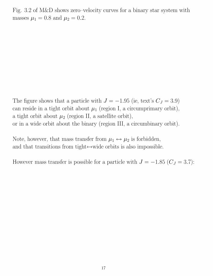
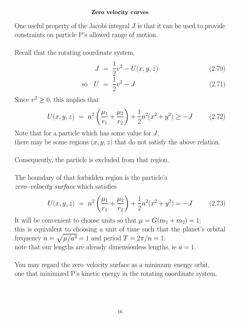
Fig. 3.2 of M&D shows zero–velocity curves for a binary star system with

masses µ1 = 0.8 and µ2 = 0.2.

The figure shows that a particle with J = −1.95 (ie, text’s CJ = 3.9)

can reside in a tight orbit about µ1 (region I, a circumprimary orbit),

a tight orbit about µ2 (region II, a satellite orbit),

or in a wide orbit about the binary (region III, a circumbinary orbit).

Note, however, that mass transfer from µ1 ↔ µ2 is forbidden,

and that transitions from tight↔wide orbits is also impossible.

However mass transfer is possible for a particle with J = −1.85 (CJ = 3.7):

17

This graphical analysis of a particle’s zero–velocity curves tells you the

possible range of that particle’s motions.

For instance, you can use these curves to determine whether a satellite’s

orbit is always confined to the vicinity of m2,

or if it can also wander into an orbit about m1.

In particular, you can use these curves to determine if mass transfer is

possible in a binary star system.

Suppose a particle at some instant of time is sitting on a zero velocity curve.

Will that particle remain motionless at that site for all times?

Why?

If a particle is stationary at all times, then it is at a site where all the forces

on that particle (gravity + centrifugal) sum to zero; those sites are known as

the Lagrange equilibrium points.

18

Lagrange Equilibrium Points

An equilibrium point = a site where the force on a motionless particle P in

the reference frame that co–rotates with m1–m2.

P’s EOM in the rotating reference frame is from Eqn. (2.24):

r = ∇U − 2~ω × r (2.74)

where U = P’s effective potential due to gravity + centrifugal acceleration

and the right term is the Coriolis acceleration.

A particle at an equilibrium point has r = 0 and r = 0,

so these equilibria satisfy ∇U(x, y, z) = 0,

ie, ∂U/∂x = ∂U/∂y = ∂U/∂z = 0.

From Eqn. (2.30),

∂U

∂z= −n2

[

µ1

r31

+µ2

r32

]

z = 0 (2.75)

so the equilibrium points lie in the z = 0 plane.

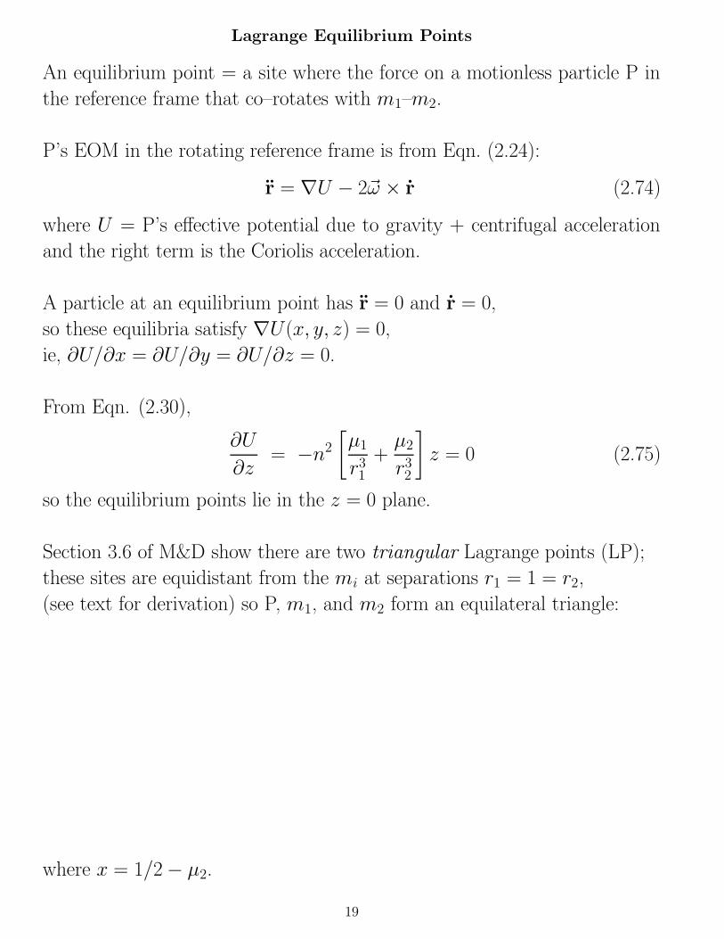
Section 3.6 of M&D show there are two triangular Lagrange points (LP);

these sites are equidistant from the mi at separations r1 = 1 = r2,

(see text for derivation) so P, m1, and m2 form an equilateral triangle:

where x = 1/2 − µ2.

19

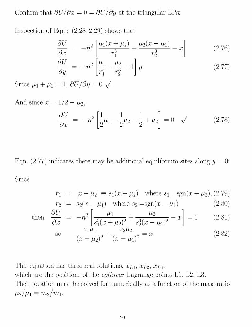
Confirm that ∂U/∂x = 0 = ∂U/∂y at the triangular LPs:

Inspection of Eqn’s (2.28–2.29) shows that

∂U

∂x= −n2

[

µ1(x + µ2)

r31

+µ2(x − µ1)

r32

− x

]

(2.76)

∂U

∂y= −n2

[

µ1

r31

+µ2

r32

− 1

]

y (2.77)

Since µ1 + µ2 = 1, ∂U/∂y = 0√

.

And since x = 1/2 − µ2,

∂U

∂x= −n2

[

1

2µ1 −

1

2µ2 −

1

2+ µ2

]

= 0√

(2.78)

Eqn. (2.77) indicates there may be additional equilibrium sites along y = 0:

Since

r1 = |x + µ2| ≡ s1(x + µ2) where s1 =sgn(x + µ2), (2.79)

r2 = s2(x − µ1) where s2 =sgn(x − µ1) (2.80)

then∂U

∂x= −n2

[

µ1

s31(x + µ2)2

+µ2

s32(x − µ1)2

− x

]

= 0 (2.81)

sos1µ1

(x + µ2)2+

s2µ2

(x − µ1)2= x (2.82)

This equation has three real solutions, xL1, xL2, xL3,

which are the positions of the colinear Lagrange points L1, L2, L3.

Their location must be solved for numerically as a function of the mass ratio

µ2/µ1 = m2/m1.

20

Fig. 3.9 of M&D shows zero–velocity curves for a secondary

of mass µ2 = 0.01.

Always keep in mind that zero–velocity curves are not orbits;

rather, they are boundaries that cannot be crossed

by a low–energy particle having a particular J .

Recall that an equilibrium point is a site where all the forces

(here, gravity + centrifugal) sum to zero.

A stable equilibrium point is a site where,

if a particle at equilibrium is displaced slightly,

then the forces cause that particle to oscillate about equilibrium.

Friction would also drive the particle back into the equilibrium.

But at an unstable equilibrium point,

the forces on a displaced particle drive it further away from equilibrium.

According to Fig. 3.9, which LP’s are stable, and which are unstable? Why

Section 3.7 examines rigorously the stability of particles at the LP’s;

and shows that L4, L5 are stable when µ2 . 0.04 (about 40 Jupiter masses).

If you displace a particle slightly from L4 or L5,

it will oscillate about that site in a tadpole orbit (green).

Such objects are sometimes called Trojans, since Jupiter’s Trojan asteroids

are the most famous example of bodies in tadpole orbits; see Fig. 3.23.

Neptune also has a few Trojans; they resemble icy Kuiper Belt Objects.

Trojans also occur in the Saturnian system:

For example, Tethys (D ∼ 1000 km) has Telesto @L and Calypso @L5; these

small satellites have D ∼ 20 km.

21

Section 3.7 shows that the L1, L2, L3 points are always unstable.

If a particle is displaced slightly from L3, it enters what resembles a

horseshoe orbit (blue) in this rotating reference frame.

Note that the horseshoe orbits circumscribe the tadpole orbits.

Objects in horseshoe or tadpole orbits are known as coorbitals,

since their motion relative to the secondary is usually quite slow.

An interesting coorbital pair are the Saturnian satellites Janus & Epimetheus.

Their masses are mepi ' 0.25mjanus,

so they seem to violate the spirit of the R3BP...

22

Note the zero velocity curve that passes through the unstable equilibria L1

and L2; recall that a level curve that passes through an unstable site is a

separatrix, which is a barrier that divides the different kinds of motion.

If a particle is displaced inwards from L1, it will orbit the primary µ1.

If displaced outwards from L1, it will orbit µ2.

Similarly, the L2 sites separates satellite orbits from circumbinary orbits.

You can think of L1 and L2 as narrow ‘gates’ or ‘keyholes’ through with a

particle can transit from circumplanetary↔circumstellar orbits.

The example of Comet Shoemake–Levy 9...

The Hill Sphere and the Roche Limit

The Hill sphere = volume around m2 interior to the LP’s L1 and L2.

This the volume where satellite orbits are stable,

and escape to a circumstellar orbit is forbidden.

The radius of the Hill sphere, RH , is very important dynamical parameter.

For instance, if you are interested in the motion of a satellite orbiting m2 at

distances of r2 RH , then you can often ignore the Sun’s gravity. This is

because the satellite is deep within m2 potential well,

and its motion is essentially 2–body motion.

However if the satellite is in a wide orbit around m2 such that r2 ∼ RH ,

then you cannot ignore the Sun, and you must treat this as a 3–body problem.

Similarly, if particle P is in a low–energy orbit about the primary m1, and

it approaches m2 to within a distance r2 ∼ RH , then large changes in P’s

orbit are likely. These encounters are known as gravitational scattering.

23

But if the separations stay large, ie, r2 RH , then the effects of gravita-

tional scattering is weak, and only small orbit changes occur (usually)...

RH is also applicable to binary star systems.

For example, RH determines the volume in which planets might orbit m2.

Or if star m2 expands beyond its Hill sphere,

then m2 can shed some mass!

Assignment #2, continueddue Thursday February 2

at the start of class

5. Use Eqn. (2.82) to show that a low mass secondary (m2 m1)

has a Hill radius

RH '(

m2

3m1

)1/3

a, (2.83)

where a is the secondary’s semimajor axis.

6. The Roche limit is usually thought of as the semimajor axis aR where the

primary’s gravitational tide just exceeds the secondary’s self–gravity, which

causes the secondary to lose mass.

The Roche limit can also be regarded as the semimajor axis aR of a body

whose physical radius just exceeds its Hill radius RH . Supposing that the

primary and secondary are uniform spheres, show that this definition lead to

a Roche limit of

aR =

(

3ρ1

ρ2

)1/3

R1 = 1.44

(

ρ1

ρ2

)1/3

R1 (2.84)

where R1 is the primary’s radius.

24

Actually, assuming m2 is a uniformly dense sphere is a poor approximation,

since m1’s tide will distort m2.

Also, the densities of m1 and m2 (which could be a planet or star) are not

uniform.

An improved solution is obtained by allowing m2 to be tidally distorted, yet

in hydrostatic equilibrium; that alters the numerical coefficient 1.44 → 2.45.

Also, if m2 is a rocky or icy satellite,

then its tensile strength resists tidal disruption,

which effectively pushes aR inwards and closer to the primary.

Nonetheless, it is worth noting that all of the major planet’s satellites

reside at a & aR, while all the planetary rings reside at a . aR.

However, small (R . 10 km) satellites can be found inside the giant planets’

Roche limits.

An example is Pan, which orbits in Saturn’s main A ring,

which is close to or interior to Saturn’s Roche limit.

25

Hill’s Equations

Hill’s eqn’s were derived by G. Hill in 1878,

are are another linearized set of EOM for the R3BP, but with the

origin moved away from the system’s COM and onto the secondary µ2.

Moving the origin to µ2 allows us to study the motion of particles as they

are perturbed by a nearby planet/satellite.

These EOM are especially useful in planetary dynamics, and can be used to

study:

• the motion of planetary ring particles perturbed by a nearby satellite,

• the accretion of a planet from a swarm of lower–mass bodies,

• the formation of binaries in the Kuiper Belt.

These EOM also have astrophysical applications, since they have been used

to study the wake (or disturbance) that a massive body (a star, or a giant

molecular cloud) generates as it travels through a galaxy.

Recall that the motion of particle P’s guiding center

resembles the zero–velocity curves (ZVC).

26

The exact EOM for the coplanar problem, Eq. (2.28), is

x = 2ny − n2

[

µ1(x + µ2)

r31

+µ2(x − µ1)

r32

− x

]

(2.85)

y = −2nx − n2

[

µ1

r31

+µ2

r32

− 1

]

y (2.86)

where r1 =√

(x + µ2)2 + y2 (2.87)

and r2 =√

(x − µ1)2 + y2 (2.88)

and all lengths are in units of the secondary’s semimajor axis a.

Lets move the origin to µ2, so x = µ1 + x′ where

x′, y′ is P’s position relative to µ2.

Our moving origin now co–rotates with the secondary,

such that the x′ direction points radially away from µ1,

and y′ points in the direction of µ2’s motion.

In the planetary approximation, µ1 ' 1 and µ2 µ1, and

r1 =√

(1 + x′)2 + y′2 '√

1 + 2x′ ' 1 + x′ (2.89)

so r−31 ' 1 − 3x′ (2.90)

and x′ ' 2ny′ − n2

[

(1 + x′)(1 − 3x′) +µ2x

′

∆3− 1 − x′

]

(2.91)

' 2ny′ + n2[

3 − µ2

∆3

]

x′ (2.92)

y′ ' −2nx′ + n2[

3x′ − µ2

∆3

]

y′ (2.93)

where ∆′ =√

x′2 + y′2 = r2.

27

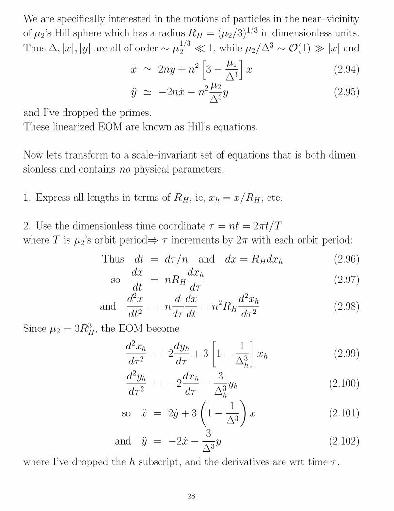
We are specifically interested in the motions of particles in the near–vicinity

of µ2’s Hill sphere which has a radius RH = (µ2/3)1/3 in dimensionless units.

Thus ∆, |x|, |y| are all of order ∼ µ1/32 1, while µ2/∆3 ∼ O(1) |x| and

x ' 2ny + n2[

3 − µ2

∆3

]

x (2.94)

y ' −2nx − n2 µ2

∆3y (2.95)

and I’ve dropped the primes.

These linearized EOM are known as Hill’s equations.

Now lets transform to a scale–invariant set of equations that is both dimen-

sionless and contains no physical parameters.

1. Express all lengths in terms of RH , ie, xh = x/RH , etc.

2. Use the dimensionless time coordinate τ = nt = 2πt/T

where T is µ2’s orbit period⇒ τ increments by 2π with each orbit period:

Thus dt = dτ/n and dx = RHdxh (2.96)

sodx

dt= nRH

dxh

dτ(2.97)

andd2x

dt2= n

d

dτ

dx

dt= n2RH

d2xh

dτ 2(2.98)

Since µ2 = 3R3H , the EOM become

d2xh

dτ 2= 2

dyh

dτ+ 3

[

1 − 1

∆3h

]

xh (2.99)

d2yh

dτ 2= −2

dxh

dτ− 3

∆3h

yh (2.100)

so x = 2y + 3

(

1 − 1

∆3

)

x (2.101)

and y = −2x − 3

∆3y (2.102)

where I’ve dropped the h subscript, and the derivatives are wrt time τ .

28

Note that µ2 has disappeared from the problem, which means that these

EOM apply to any R3BP (provided µ2 1 of course),

ie, to binary stars having extreme mass ratios, the Pluto–Charon binary,

satellites of the giant planets, etc.

We will use Hill’s equations later in a more detailed examination of planetary

rings.

Assignment #2, continueddue Thursday February 2

at the start of class

7. Show that the scale–invariant Hill eqn’ for a particle’s vertical motion is

z = −(

1 +3

∆3

)

z (2.103)

where ∆ = the particle’s distance from m2 in Hill units.

8. Start with the scale–invariant Hill eqn’s, and derive a new Jacobi integral

Jh =1

2v2 − Uh, (2.104)

Uh(x, y, z) =3

2x2 − 1

2z2 +

3

∆, (2.105)

where v is the particle’s velocity in Hill units,

and Uh is the new effective potential in these units.

29

Fig. 3.30 shows the results of a numerical integration of Hill’s eqns for

numerous particles P initially in circular orbits having a wide range of

impact parameters x = (ap − a)/RH .

First, note that Hill’s approximation essentially removes the curvature of a

circular orbit, thus unperturbed particles would move left↔right.

As expected, Ps with impact parameters |x| . 1 are in horseshoe orbits,

while more distant Ps get more strongly perturbed, and enter higher e orbits.

But why don’t we see the effects of the triangular Lagrange points in this

diagram?

Evidently, Hill’s eqn’s break down as the Ps drift to large longitudes y 1.

Where is periapse and apoapse in this diagram?

Which trajectories might correspond to ones that might collide with µ2?

Also note the wavelike streamline in the more distant post–encounter

trajectories, which are known as wakes.

Voyager saw wakes in Saturn’s rings (see Fig 10.21—10.23), which were

used to pinpoint the location of the previously unknown satellite Pan, which

is ∼ 25 km. Pan’s wakes are seen quite prominently in the newer Cassini

images of the rings.

On the class website I have posted an animation of a numerical solution to

Hill’s equations for a swarm of ring particles that encounter a satellite. The

particles start on circular orbits, and the animation shows horseshoe orbits,

wakes, and scattered particles.

30

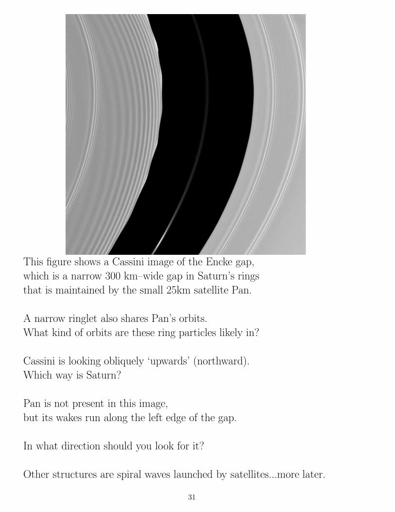
This figure shows a Cassini image of the Encke gap,

which is a narrow 300 km–wide gap in Saturn’s rings

that is maintained by the small 25km satellite Pan.

A narrow ringlet also shares Pan’s orbits.

What kind of orbits are these ring particles likely in?

Cassini is looking obliquely ‘upwards’ (northward).

Which way is Saturn?

Pan is not present in this image,

but its wakes run along the left edge of the gap.

In what direction should you look for it?

Other structures are spiral waves launched by satellites...more later.

31

Distant Encounters

Examine the motion of a particle that is NOT on a horseshoe orbit;

inspection of Fig. 3.30 that the encounter excites the particle’s eccentricity e.

Lets calculate that e, since it will be quantify the disturbance that a

perturber (like a moon embedded in a planetary ring, or a planet embedded

in a planet-forming disk) might excite.

The 2D Hill’s EOM are

x − 2y − 3x = − 3x

∆3(2.106)

y + 2x = − 3y

∆3(2.107)

where distance from perturber m2 is ∆ =√

x2 + y2,

all lengths are in units of RH , and the dimensionless time is τ = nt.

First consider unperturbed motion, where m2 → 0.

Since RH → 0, ∆ → 0 and RHS→ 0.

Unperturbed circular motion thus corresponds to

x(t) = b = constant (2.108)

so y = −3

2b (2.109)

and y = −3

2bt. (2.110)

where the separation is ∆ = b√

1 + (3t/2)2 ≡ ∆0(t).

We will call this the zeroth order solution.

Note that y is the particle’s angular velocity relative to m2,

so the synodic period if τsyn = 2π/y.

Does this agree with you answer to problem 3 of Assignment #1?

32

Now assume m2 6= 0, and that the encounter is distant, |b| 1

so that the perturbation is weak. Then

x(t) = b + x1(t) (2.111)

y(t) = −3

2bt + y1(t) (2.112)

Now turn on the perturbation, and linearize the EOM,

ie, assume |x1| & |y1| are |b|.

Also, when calculating the disturbance (terms on RHS of EOM),

adopt the particle’s undisturbed trajectory:

x1 − 2y1 − 3x1 = − 3b

∆30

(2.113)

y1 + 2x1 =9bt/2

∆30

(2.114)

The solution will be first–order in the perturbation.

An analytic solution for these simple–looking EOM is rather difficult...

Instead, lets obtain a quick ’n dirty solution to this problem:

Assume that P’s motion is simple 2-body epicyclic motion when far from m2,

and hyperbolic when near m2:

33

The figure shows that P is scattered by m2 through angle θs,

which you obtained in problem #3 of Assignment 1:

cos1

2(θs + π) = −1

eEqn. (1.97) (2.115)

so sin1

2θs =

1

e(2.116)

where e =√

1 + b2v4∞/µ2 Eqn. (1.95) (2.117)

is the eccentricity of the hyperbolic orbit, µ = Gm2 (why?), P’s velocity-

at-infinity relative to m2 is v∞ = 3bn/2 (why?) where n2 = Gm1/a3 (why?).

Distant encounters (ie, large b) are fast, so e 1 and

θs '2

e' 2Gm2

bv2∞

=8µ2

9

(a

b

)3

=8

3

(

RH

b

)3

(2.118)

so the scattering angle is small (as expected) when b Hill radius RH .

Recall that a hyperbolic scattering event does not alter P’s energy;

it merely alters the direction of P’s outbound velocity v,

giving it a radial velocity in the x direction:

|vx| ' v∞θs → vx ' −4µ2

3

(a

b

)2

an (2.119)

why the − sign?

Long after the encounter,

P resumes epicyclic motion about the primary m1:

r(t) ' (a + b) − (a + b)e cos nt from Eqn. (1.98) (2.120)

so r ' ean sin(nt) since |b| a. (2.121)

Since r ∼ O(vx),

this tells you that m2’s perturbation pumped P’s eccentricity up to

e ∼∣

∣

∣

∣

r

an

∣

∣

∣

∣

∼ 4

3

(a

b

)2

µ2 ' 1.33(a

b

)2

µ2 (2.122)

34

Julian & Toomre (1966) solved this problem in their study of stars in nearly

circular orbits in a disk galaxy that are perturbed by another massive body;

they provide a more exact solution to the linearized 3-body equations (2.113),

and show that long after the encounter (t → +∞), P’s radial motion is:

x1(t) → −sgn(b)8f

3b2sin τ (2.123)

(in dimensionless Hill units), where the coefficient

f = 2K0(2/3) + K1(2/3) ' 2.52 depends on modified Bessel functions Ki.

Convert this to physical units, ie, multiply lengths ×RH and replace τ → nt:

x1(t) → −sgn(b)8fµ2

9

(a

b

)2

sin(nt)a (2.124)

where a is ms’s semimajor axis.

This result was used to examine how a giant molecular cloud orbiting in a

disk galaxy can pump up the radial motions of stars.

We will use it to study how a satellite orbiting in a planetary ring,

or how a planet in a circumstellar disk will open a gap about its orbit.

This process is known as shepherding—see below.

The eccentricity e inferred from the above exact solution is

e =∣

∣

∣

x1

a

∣

∣

∣=

8f

9

(a

b

)2

µ2 ' 2.24(a

b

)2

µ2. (2.125)

which is ∼ 2 times larger that our earlier estimate.

As expected, particles having a smaller impact parameter |b| gets excited to

higher-e orbits.

35

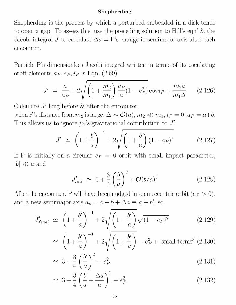
Shepherding

Shepherding is the process by which a perturbed embedded in a disk tends

to open a gap. To assess this, use the preceding solution to Hill’s eqn’ & the

Jacobi integral J to calculate ∆a = P’s change in semimajor axis after each

encounter.

Particle P’s dimensionless Jacobi integral written in terms of its osculating

orbit elements aP , eP , iP is Eqn. (2.69)

J ′ =a

aP+ 2

√

(

1 +m2

m1

)

aP

a(1 − e2

P ) cos iP +m2a

m1∆(2.126)

Calculate J ′ long before & after the encounter,

when P’s distance from m2 is large, ∆ ∼ O(a), m2 m1, iP = 0, aP = a+b.

This allows us to ignore µ2’s gravitational contribution to J ′:

J ′ '(

1 +b

a

)−1

+ 2

√

(

1 +b

a

)

(1 − eP )2 (2.127)

If P is initially on a circular eP = 0 orbit with small impact parameter,

|b| a and

J ′init ' 3 +

3

4

(

b

a

)2

+ O(b/a)3 (2.128)

After the encounter, P will have been nudged into an eccentric orbit (eP > 0),

and a new semimajor axis ap = a + b + ∆a ≡ a + b′, so

J ′final '

(

1 +b′

a

)−1

+ 2

√

(

1 +b′

a

)

√

(1 − eP )2 (2.129)

'(

1 +b′

a

)−1

+ 2

√

(

1 +b′

a

)

− e2P + small terms3 (2.130)

' 3 +3

4

(

b′

a

)2

− e2P (2.131)

' 3 +3

4

(

b

a+

∆a

a

)2

− e2P (2.132)

36

Assume the nudge is small compared to impact parameter, |∆a| |b|. Then

J ′final ' J ′

init +3

2

b

a

∆a

a− e2

P (2.133)

Since J ′ is conserved, this implies that

∆a ' sgn(b)2

3

∣

∣

∣

a

b

∣

∣

∣e2Pa (2.134)

This is sometimes called the impulse approximation,

since µ2 is impulsively nudging P’s semimajor axis away,

and nudging is eccentricity eP upwards as per Eqn. 2.125.

Problem 3 of Assignment #1 showed that P will encounter µ2 again

after one synodic period:

∆t = Tsyn =4π

3n

∣

∣

∣

a

b

∣

∣

∣(2.135)

which is many orbital periods later when |b| a.

Suppose particle P is orbiting in a disk that is crowded with many particles:

(eg, a planetary ring, or a disk galaxy composed of many stars).

Subsequent interactions can damp out P’s eccentricity:

via collisions among particles in a planetary ring,

or via dynamical friction in a galaxy due to interactions with other stars.

A suffiently massive planet still orbiting in its natal circumstellar gas disk

can also open a gap in the gas disk—why?

In such cases, P will approach µ2 again in a circular orbit

which will nudge its semimajor axis away at the average rate

a =∆a

∆t= sgn(b)

32f 2

81π

∣

∣

∣

a

b

∣

∣

∣

4

µ22an (2.136)

37

This is shepherding: the process by which perturber µ2 embedded in a dense

disk tends to open a gap in the disk about µ2’s orbit. This occurs provided

the particle’s e’s get damped prior to each encounter with µ2.

Pan orbits in the narrow Encke gap in Saturn’s rings.

What then prevents Pan from making the Encke gap ever wider?

Assignment #3due Tuesday February 14

at the start of class

1. Eqn. (2.134) was derived by assuming that the displacement |∆a| |b|.Use this equation to prove that our assumption is indeed valid when

|b| 1.8, ie, P’s impact parameter is larger than about 1.8 Hill radii.

2. Note the Encke gap’s wavy edge. Show that these so–called edge waves

have a longitudinal wavelength (ie, peak-to-peak distance) of

λ = 3πx (2.137)

where x is Pan’s distance from the gap edge.

3. Pan orbits x = 160 km from edge of the Encke gap. What is the ra-

dial amplitude of these edge waves, in units of km? Explain your calculation.

4. A small particle of mass m is in a circular orbit, and it is subject to

torque T that is normal to its orbit plane. Show that this torque drives the

particle’s semimajor axis at the rate

a =2T

man. (2.138)

Aside: recall that a small body’s total angular momentum is L = mr × r,

and that the torque on that body is

T =dL

dt= mr × r (2.139)

38

Torque Density

Suppose µ2 is now disturbing a dense ring of particles having a mass surface

density σ, orbital radius r = a + b, and narrow radial width ∆r.

Assume all e’s gets damped downstream via particle–particle interactions.

What is the mass of this ring? ∆m = σ∆A = 2πσr∆r.

What is the total torque ∆T that µ2 exerts on the ring?

∆T =1

2ana∆m (2.140)

sodT

dr= sgn(b)(πσr2)

32f 2

81π

(

a

r − a

)4

µ22an2 (2.141)

= sgn(b)32f 2

81π

(

a

r − a

)4

µdµ22m1an2 (2.142)

where µd ≡ πσr2

m1

(the so–called normalized disk mass) (2.143)

is the torque radial density,

ie dTdr

∆r = total torque that µ2 exerts on a ring of radius r and width ∆r.

39

Assignment #3, continueddue Tuesday February 14

at the start of class

5. Suppose µ2 orbits a radial distance x beyond a disk having a constant

surface density σ. Show that the total torques it exerts on the disk is

T =

∫

disk

dT

drdr ' −32f 2

243π

∣

∣

∣

a

x

∣

∣

∣

3

µdµ22m1(an)2 (2.144)

where |x| is small compared to µ2’s semimajor axis a. How will the disk

respond to µ2’s perturbations? How will µ2’s orbit to evolve over time?

6. Suppose µ2 formed at the outer edge of a disk of radius a, and that

the shepherding torques have since driven radially outwards a small distance

x a. Show that µ2’s travel–time t is

t ' 243π

256f 2

∣

∣

∣

x

a

∣

∣

∣

4 1

µdµ2n(2.145)

7. The small satellite Prometheus orbits x = 2570km beyond the outer

edge of Saturn’s main A ring, which has a mass surface density of σ ∼ 100

gm/cm2. Suppose Prometheus formed at the ring edge. How long ago

did that happen, in years? How many orbital periods is that? What

does this calculation tell you about the age of this part of the ring system

and the nearby satellite? (Actually, your age estimate is merely a lower

limit on the true age...). See Appendix A of M&D for planet & satellite data.

We will use the above calculations again later when we study the dynamics

of recently–formed planets that are interacting with a circumstellar gas disk.

40

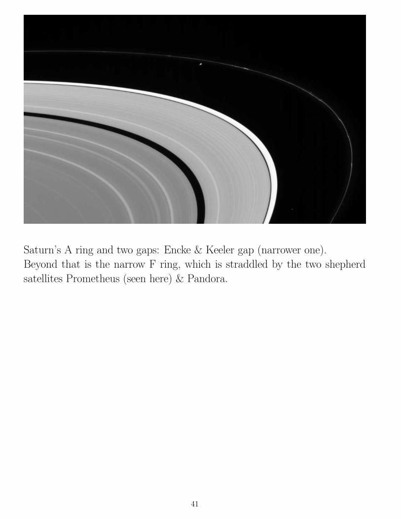
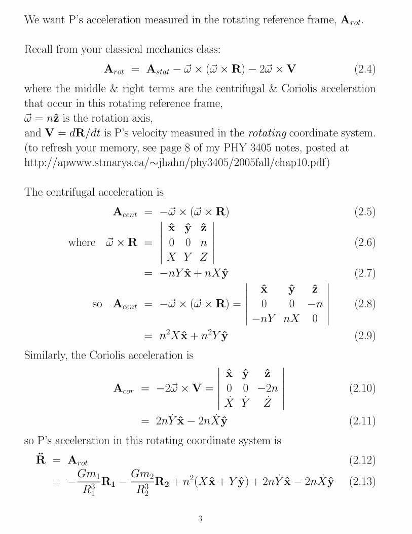
Saturn’s A ring and two gaps: Encke & Keeler gap (narrower one).

Beyond that is the narrow F ring, which is straddled by the two shepherd

satellites Prometheus (seen here) & Pandora.

41