2D Finite Difference Method - my.civil.utah.edubartlett/CVEEN 7330/2D Finite Difference...

© Steven F. Bartlett, 2011

Course Information○

Lecture Notes○

Pp. 73 - 75 Kramer○

Reading Assignment

FLAC User Manual Theory and Background, Section 1 - Background -The Explicit Finite Difference Method

○

Other Materials

Homework Assignment #6

Complete CVEEN 7330 Modeling Exercise 1 (in class)1.Complete CVEEN 7330 Modeling Exercise 2 (30 points - plot, 10 points other

calculations and discussion)

2.

2D Finite Difference MethodSunday, August 14, 20113:32 PM

2D Finite Difference Method

Steven F. Bartlett, 2010

Modeling Steps for Applying Finite Difference Method

Generate a grid for the domain where we want an approximate solution.1.Assign material properties to the model (density, shear and bulk modulus)2.

fixed versus freea.Assign boundary conditions3.

for dynamic modeling this is usually assigned at the base as a velocity

time history

a.apply loading conditions4.

Use the finite difference equations as a substitute for the ODE/PDE system

of equations. The ODE/PDE, thus substituted, becomes a linear or non-linear system of algebraic equations that can be solved incrementally with

time

5.

Solve for the system of algebraic equations using the initial conditions and

the boundary conditions. This usually done by time stepping in an explicit formulation.

6.

Implement the solution in computer code to perform the calculations.7.Interpret the results8.Check the results with known solutions, if possible9.

Finite Difference MethodThursday, March 11, 201011:43 AM



Grid GenerationThursday, March 11, 201011:43 AM



The finite difference grid also identifies the storage location of all state variables in the model. The procedure followed by FLAC is that all vector quantities (e.g.. forces. velocities. displacements. flow rates) are stored at gridpoint locations. while all scalar and tensor quantities (e.g.. stresses. pressure. material properties) are stored at zone centroid locations. There are three exceptions: saturation and temperature are considered gridpoint variables: and pore pressure is stored at both gridpoint and zone centroid locations.

Grid Generation (continued)Thursday, March 11, 201011:43 AM



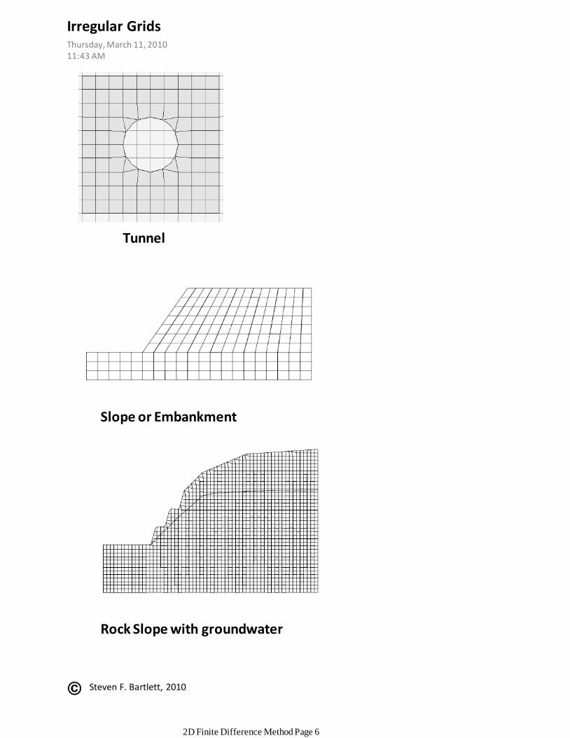
Tunnel

Slope or Embankment

Rock Slope with groundwater

Irregular GridsThursday, March 11, 201011:43 AM



Braced Excavation

Concrete Diaphragm Wall

Irregular grids (cont.)Thursday, March 11, 201011:43 AM



Elastic and Mohr Coulomb ModelsDensity•Bulk Modulus•Shear Modulus•Cohesion (MC only)•Tension (MC only)•Drained Friction Angle (MC only)•Dilation Angle (MC only)•

Hyperbolic Model

Required Input for Hyperbolic Model

Function Form of Hyperbolic Model

Material PropertiesThursday, March 11, 201011:43 AM



FLAC accepts any consistent set of engineering units. Examples of consistent sets of units for basic parameters are shown in Tables 2.5. 2.6 and 2.7. The user should apply great care when converting from one system of units to another. No conversions are performed in FLAC except for friction and dilation angles. which are entered in degrees.

Units for FLACThursday, March 11, 201011:43 AM



Positive = tension○

Negative = compression○

Normal or direct stress

Shear stress

With reference to the above figure, a positive shear stress points in the positive direction of the coordinate axis of the second subscript if it acts on a surface with an outward normal in the positive direction. Conversely, if the outward normal of the surface is in the negative direction, then the positive shear stress points in the negative direction of the coordinate axis of the second subscript. The shear stresses shown in the above figure are all positive (from FLAC manual).

In other words, xy is positive in the counter-clockwise direction;

likewise yx is positive in the clockwise direction.

Sign Conventions for FLACThursday, March 11, 201011:43 AM


DIRECT OR NORMAL STRAIN

Positive strain indicates extension: negative strain indicates compression.

○

SHEAR STRAIN

Shear strain follows the convention of shear stress (see figure above). The distortion associated with positive and negative shear strain is illustrated in Figure 2.44.

○

PRESSURE

A positive pressure will act normal to. and in a direction toward. the surface of a body (i.e.. push), A negative pressure will act normal to. and in a direction away from. the surface of a body (i.e.. pull). Figure 2.45 illustrates this convention.

○


Sign Conventions (cont.)Thursday, March 11, 201011:43 AM



PORE PRESSURE

Fluid pore pressure is positive in compression. Negative pore pressure indicates fluid tension.

○

GRAVITY

Positive gravity will pull the mass of a body downward (in the negative y-direction). Negative gravity will pull the mass of a body upward.

○

GFLOW

This is a FISH parameter (see Section 2 in the FISH volume which denotes the net fluid flow associated with a gridpoint. A positive gflow corresponds to flow into a gridpoint. Conversely, a negative gflow corresponds to flow out of a gridpoint.

○

Sign Conventions (cont.)Thursday, March 11, 201011:43 AM



Boundary Conditions

Fixed (X or Y) or both (B)○

Free○

Applied Conditions at Boundary

Velocity or displacement○

Stress or force○

X means fixed in x direction

B means fixed in both directions

Yellow line with circle means force, velocity or stress has been applied to this surface.

Boundary ConditionsThursday, March 11, 201011:43 AM



Finite-difference methods approximate the solutions to differential equations by replacing derivative expressions with approximately equivalent difference quotients. That is, because the first derivative of a function f is, by definition,

then a reasonable approximation for that derivative would be to take

for some small value of h. In fact, this is the forward differenceequation for the first derivative. Using this and similar formulae to replace derivative expressions in differential equations, one can approximate their solutions without the need for calculus

Pasted from <http://en.wikipedia.org/wiki/Finite_difference_method>

Only three forms are commonly considered: forward, backward, and central differences.A forward difference is an expression of the form

Depending on the application, the spacing h may be variable or held constant.A backward difference uses the function values at x and x − h, instead of the values at x + h and x:

Finally, the central difference is given by

Pasted from <http://en.wikipedia.org/wiki/Forward_difference >

Fundamentals of FDMThursday, March 11, 201011:43 AM


http://en.wikipedia.org/wiki/Difference_quotient

http://en.wikipedia.org/wiki/Derivative#Definition_via_difference_quotients

http://en.wikipedia.org/wiki/Forward_difference#Forward.2C_backward.2C_and_central_differences

http://en.wikipedia.org/wiki/Finite_difference_method

http://en.wikipedia.org/wiki/Forward_difference


Higher-order differences

2nd Order Derivative

In an analogous way one can obtain finite difference approximations to higher order derivatives and differential operators. For example, by using the above central difference formula for f'(x + h / 2) and f'(x − h/ 2) and applying a central difference formula for the derivative of f' at x, we obtain the central difference approximation of the second derivative of f:

Pasted from <http://en.wikipedia.org/wiki/Finite_difference >

Examples

Pasted from <http://en.wikipedia.org/wiki/Groundwater_flow_equation >

Groundwater flow equation

Pasted from <https://ccrma.stanford.edu/~jos/pasp/D_Mesh_Wave.html>

2D wave equation

Fundamentals of FDM (cont.)Thursday, March 11, 201011:43 AM


http://en.wikipedia.org/wiki/Finite_difference

http://en.wikipedia.org/wiki/Groundwater_flow_equation

https://ccrma.stanford.edu/~jos/pasp/D_Mesh_Wave.html


Explicit and implicit methods are approaches used in numerical analysisfor obtaining numerical solutions of time-dependent ordinary and partial differential equations, as is required in computer simulations of physical processes.

Explicit methods calculate the state of a system at a later time from the state of the system at the current time, while implicit methods find a solution by solving an equation involving both the current state of the system and the later one. Mathematically, if Y(t) is the current system state and Y(t + Δt) is the state at the later time (Δt is a small time step), then, for an explicit method

while for an implicit method one solves an equation

to find Y(t + Δt).

It is clear that implicit methods require an extra computation (solving the above equation), and they can be much harder to implement. Implicit methods are used because many problems arising in real life are stiff, for which the use of an explicit method requires impractically small time steps Δt to keep the error in the result bounded (see numerical stability). For such problems, to achieve given accuracy, it takes much less computational time to use an implicit method with larger time steps, even taking into account that one needs to solve an equation of the form (1) at each time step. That said, whether one should use an explicit or implicit method depends upon the problem to be solved.

Pasted from <http://en.wikipedia.org/wiki/Explicit_method>

Fundamentals of FDM - Explicit vs Implicit MethodsThursday, March 11, 201011:43 AM


http://en.wikipedia.org/wiki/Numerical_analysis

http://en.wikipedia.org/wiki/Ordinary_differential_equation

http://en.wikipedia.org/wiki/Partial_differential_equation

http://en.wikipedia.org/wiki/Computer_simulation

http://en.wikipedia.org/wiki/Process_%28science%29

http://en.wikipedia.org/wiki/Stiff_equation

http://en.wikipedia.org/wiki/Numerical_stability

http://en.wikipedia.org/wiki/Numerical_stability

http://en.wikipedia.org/wiki/Explicit_method


The previous page contains explains the explicit method which is implemented in FLAC. The central concept of an explicit method is that the calculational “wave speed” always keeps ahead of the physical wave speed, so that the equations always operate on known values that are fixed for the duration of the calculation. There are several distinct advantages to this (and at least one big disadvantage!): most importantly, no iteration process is necessary. Computing stresses from strains in an element, even if the constitutive law is wildly nonlinear.

In an implicit method (which is commonly used in finite element programs), every element communicates with every other element during one solution step: several cycles of iteration are necessary before compatibility and equilibrium are obtained.

Table 1.1 (next page) compares the explicit amid implicit methods. The disadvantage of the explicit method is seen to be the small timestep, which means that large numbers of steps must be taken. Overall, explicit methods are best for ill-behaved systems e.g., nonlinear, large—strain, physical instability; they are not efficient for modeling linear, small—strain problems.

Explicit versus Implicit FormulationThursday, March 11, 201011:43 AM



Table 1.1 Comparison of Explicit versus Implicit Formulations

Explicit

Timestep must be smaller than a critical value for stability

•

Small amount of computational effort per timestep.

•

No significant numerical damping introduced for dynamic solution

•

No iterations necessary to follow nonlinear

•

constitutive law.Provided that the timestep criterion is always satisfied, nonlinear laws are always followed in a valid physical way.

•

Matrices are never formed. •Memory requirements are always at a minimum. No bandwidth limitations.

•

Since matrices are never formed large displacements and strains are accommodated without additional computing effort.

Implicit

Timestep can be arbitrarily large with unconditionally stable schemes

•

Large amount of computational effort per timestep.

•

Numerical damping dependent on timestep present with unconditionally stable schemes.

•

Iterative procedure necessary to follow nonlinear constitutive law.

•

Always necessary to demonstrate that the above-mentioned procedure is: (a) stable: and (b) follows the physically correct path (for path-sensitive problems).

•

Stiffness matrices must be stored. Ways must be found to overcome associated problems such as bandwidth.

•

Memory requirements tend to be large.

•

Additional computing effort needed to follow large displacements and strains.

•

Explicit versus Implicit Formulation (cont.)Thursday, March 11, 201011:43 AM


Explicit, Time-Marching Scheme

Even though we want FLAC to find a static solution to a problem, the dynamic

equations of motion are included in the formulation. One reason for doing this is to ensure that the numerical scheme is stable when the physical system being

modeled is unstable. With nonlinear materials, there is always the possibility of physical instability—e.g., the sudden collapse of a pillar. In real life, some of the

strain energy in the system is converted into kinetic energy, which then radiates away from the source and dissipates. FLAC models this process directly, because

inertial terms are included — kinetic energy is generated and dissipated. In contrast, schemes that do not include inertial terms must use some numerical

procedure to treat physical instabilities. Even if the procedure is successful at preventing numerical instability, the path taken may not be a realistic one. One

penalty for including the full law of motion is that the user must have some physical feel for what is going on; FLAC is not a black box that will give “the

solution.” The behavior of the numerical system must be interpreted.


Explicit Method Used in FLACThursday, March 11, 201011:43 AM



Lagrangian analysis is the use of Lagrangian coordinates to analyze various

problems in continuum mechanics.

Lagrangian analysis may be used to analyze currents and flows of various

materials by analyzing data collected from gauges/sensors embedded in the material which freely move with the motion of the material.[1] A common

application is study of ocean currents in oceanography, where the movable gauges in question called Lagrangian drifters.

Pasted from <http://en.wikipedia.org/wiki/Lagrangian_analysis>

Pasted from <http://www.ansys.com/products/images/new-

features-1.jpg>

Since FLAC does not need to form a global stiffness matrix, it is a trivial matter

to update coordinates at each timestep in large-strain mode. The incremental displacements are added to the coordinates so that the grid moves and deforms

with the material it represents. This is termed a “Lagrangian” formulation. in contrast to an “Eulerian” formulation. in which the material moves and deforms

relative to a fixed grid. The constitutive formulation at each step is a small—strain one, but is equivalent to a large-strain formulation over many steps.

Example of Lagrangian analysis of golf club head striking ball. Note that the tracking and movement of the sand with the striking of the ball requires a Lagrangian analysis. (from ANSYS)

Lagrangian AnalysisThursday, March 11, 201011:43 AM


http://en.wikipedia.org/wiki/Lagrangian_and_Eulerian_specification_of_the_flow_field

http://en.wikipedia.org/wiki/Fluid_dynamics

http://en.wikipedia.org/wiki/Fluid_dynamics

http://en.wikipedia.org/wiki/Lagrangian_analysis#cite_note-0

http://en.wikipedia.org/wiki/Ocean_current

http://en.wikipedia.org/wiki/Oceanography

http://en.wikipedia.org/wiki/Lagrangian_drifter

http://en.wikipedia.org/wiki/Lagrangian_analysis

http://www.ansys.com/products/images/new-features-1.jpg

http://www.ansys.com/products/images/new-features-1.jpg


Eq. (1.1)

Note that the above partial differential equation is a 2nd order partial differential

equation because u dot is a derivative of u (displacement). This equation expresses dynamic force equilibrium which relates the inertial and gravitational

forces to changes in stress. It is essentially the wave equation, which is further discussed in soil dynamics.

Equation of MotionThursday, March 11, 201011:43 AM



The constitutive relation that is required in the PDE given before relates changes

in stress with strain.

However, since FLAC's formulation is essentially a dynamic formulation, where

changes in velocities are easily calculated, then strain rate is used and is related to velocity as shown below.

The mechanical constitutive law has the form:

Constitutive RelationsThursday, March 11, 201011:43 AM



Stress Strain Constitutive Law (Hooke's

Law)

Equation of Motion for Dynamic

Equilibrium (wave equation)

Eq. (1.2)FDM formulation using central finite

difference equation.

The central finite difference equation corresponding is for a typical zone i is given

by the above equation. Here the quantities in parentheses — e.g.. (i) — denote the time, t, at which quantities are evaluated: the superscripts. i, denote the zone

number, not that something is raised to a power.

Numbering scheme for a 1-D body using FDM.

FDM - Elastic Example from FLAC manualThursday, March 11, 201011:43 AM



Finite difference equation for equation of motion using central finite difference

equation. Note that on the left side of the equation a change in velocity (i.e., acceleration) is represented; on the right side of the equation a change in stress

with respect to position is represented for the time step. In other words, an acceleration (unbalanced force) causes a change is the stress, or stress wave.

Rearrange the above equation, produces Eq. 1.3

Integrating this equation, produces displacements as shown in Eq. 1.4

This equation says that the position and time t + delta t is equal to the position

and time t + (velocity at time t + 1/2 delta t) * delta t.

FDM - Elastic Example (cont.)Thursday, March 11, 201011:43 AM



In the explicit method. the quantities on the right-hand sides of all difference

equations are “known”; therefore. we must evaluate Eq. 1.2) for all zones before moving on to Eqs. (1.3) and (1.4). which are evaluated for all grid points.

Conceptually. this process is equivalent to a simultaneous update of variables.

motion

bc velocity pulse applied to boundary condition dis_calc displacements from velocity constit stresses are derived from strain motion velocity calculated stress

dis_calc

constit

bc




The following is an example of implementing the FDM for to calculate the

behavior of an elastic bar. To do this, we must write FISH code. The primary subroutine, scan_all, and the other routines described in the following pages can

be obtained from bar.dat in the Itasca folder.

def scan_all while_stepping time = time + dt bc ; pulse applied to boundary condition dis_calc ; displacements calculated from velocity constit ; stresses are derived from strain motion ; velocity calculated stressend

def bc ; boundary conditions - cosine pulse applied to left end if time >= twave then xvel(1,1) = 0.0 else xvel(1,1) = vmax * 0.5 * (1.0 - cos(w * time)) end_ifEnd

The subroutine, dis_calc, calculates the displacements from the velocities.

The subroutine, bc, applies a one-sided cosine velocity pulse to the left end of the

rod.

def dis_calc loop i (1,nel) xdisp(i,1) = xdisp(i,1) + xvel(i,1) * dtend_loop end




The subroutine, called constit, calculates the stress as derived from strain using

Hooke's law. The value of e is Young's modulus.

def motion loop i (2,nel) xvel(i,1) = xvel(i,1) + (sxx(i,1) - sxx(i-1,1)) * tdx end_loop end

def constit loop i (1,nel) sxx(i,1) = e * (xdisp(i+1,1) - xdisp(i,1)) / dx end_loop end

This subroutine, called motion, calculates the new velocity from stress. Recall

that an unbalanced stress causes an unbalanced force, which in turn produces an acceleration which is a change in velocity.



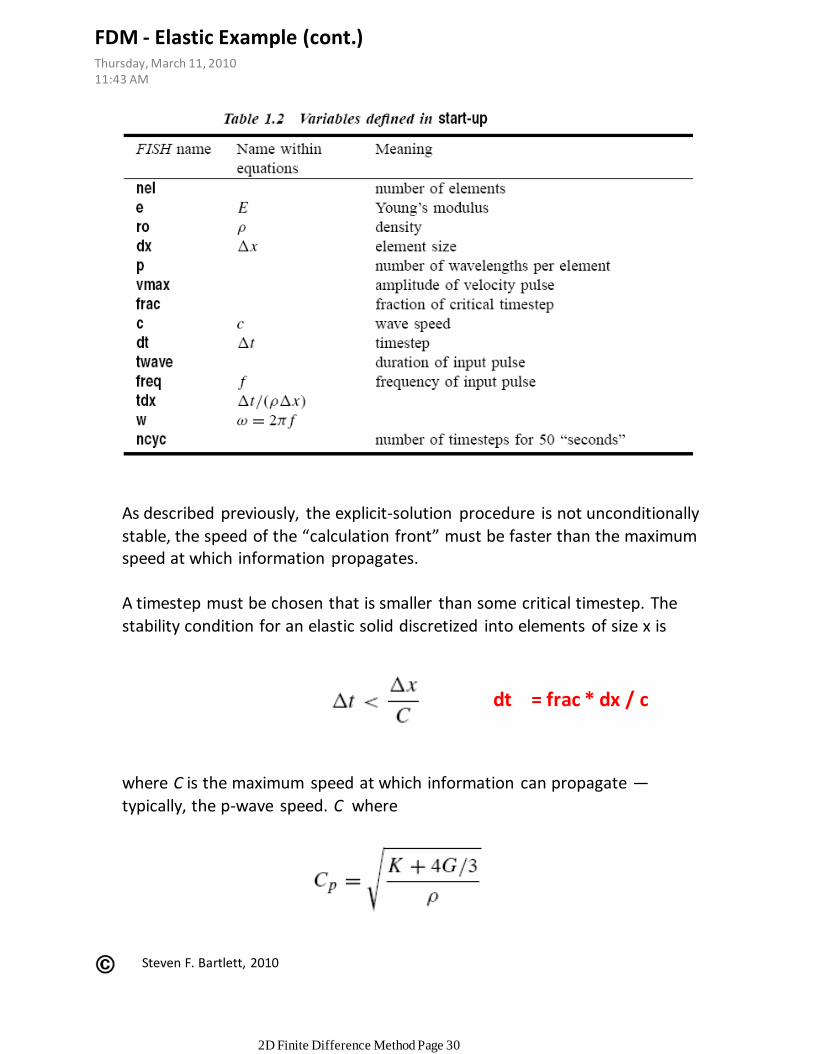
As described previously, the explicit-solution procedure is not unconditionally

stable, the speed of the “calculation front” must be faster than the maximum speed at which information propagates.

A timestep must be chosen that is smaller than some critical timestep. The

stability condition for an elastic solid discretized into elements of size x is

where C is the maximum speed at which information can propagate —

typically, the p-wave speed. C where

dt = frac * dx / c





nel = 50 ; no. of elements e = 1.0 ; Young's modulus ro = 1.0 ; density dx = 1.0 ; element size p = 15.0 ; number of wavelengths per elements vmax = 1.0 ; amplitude of velocity pulse frac = 0.2 ; fraction of critical timestep

FDM - Elastic Example (cont.) - SolutionThursday, March 11, 201011:43 AM


2D Finite Difference Method - my.civil.utah.edubartlett/CVEEN 7330/2D Finite Difference...

Documents

Transcript of 2D Finite Difference Method - my.civil.utah.edubartlett/CVEEN 7330/2D Finite Difference...